TWISTING THE ALIVE PARTICLE FILTER
Adam Persing1 and Ajay Jasra2
1Department of Mathematics, Imperial College London
2Department of Statistics & Applied Probability, National University of Singapore
Abstract: This work focuses on sampling from hidden Markov models [3] whose observations have intractable density functions. We develop a new sequential Monte Carlo ([6], [10], [11]) algorithm and a new particle marginal Metropolis-Hastings [2] algorithm for these purposes. We build from [13] and [23] to construct the sequential Monte Carlo (SMC) algorithm (which we call the alive twisted particle filter). Like the alive particle filter of [13], our new SMC algorithm adopts an approximate Bayesian computation [22] estimate of the HMM. Our alive twisted particle filter also uses a twisted proposal as in [23] to obtain a low-variance estimate of the HMM normalising constant. We demonstrate via numerical examples that, in some scenarios, this estimate has a much lower variance than that of the estimate obtained via the alive particle filter. The low variance of this normalising constant estimate encourages the implementation of our SMC algorithm within a particle marginal Metropolis-Hastings (PMMH) scheme, and we call the resulting methodology “alive twisted PMMH”. We numerically demonstrate on a stochastic volatility model how our alive twisted PMMH can converge faster than the standard alive PMMH of [13].
Key words and phrases: Alive particle filters, approximate Bayesian computation, hidden Markov models, particle Markov chain Monte Carlo, sequential Monte Carlo, twisted particle filters.
1. Introduction
Consider a Markov process that evolves in discrete time, and assume that we cannot directly observe the states of the process. At each time point, we can only indirectly observe the latent state through some other random variable. Assume also that the observation random variables are statistically independent of one another, conditioned upon the latent Markov process at the current state. This model is called a hidden Markov model [3]. Hidden Markov models (HMMs) are very flexible, and so they are used in a wide array of real world applications. Some examples include stochastic volatility models [17], real-time hand writing recognition [12], and DNA segmentation [19].
As increasing amounts of data have become available to practitioners, real world HMMs have become more and more complex; see [5], [20] and [24] for examples. In instances where analytical Bayesian inference for an HMM is not feasible, one may resort to numerical methods, such as the extended Kalman filter [1], the unscented Kalman filter [15], block updating Markov chain Monte Carlo [21], sequential Monte Carlo ([6],[10],[11]), and particle Markov chain Monte Carlo [2]. The latter two methods are widely regarded as the state-of-the-art, and we further discuss the details of those techniques in Sections 4 and 8 below. We briefly say here that sequential Monte Carlo (SMC) is a popular class of algorithms that simulate a collection of weighted samples (or “particles”) of the HMM’s hidden state sequentially in time by combining importance sampling and resampling techniques. SMC algorithms can be implemented online, and they can be used to obtain unbiased estimates of the probability density of the HMM’s observations given the model parameters (i.e., the marginal likelihood). Particle marginal Metropolis-Hastings (PMMH) algorithms (a type of particle Markov chain Monte Carlo) employ SMC and an unbiased estimate of the marginal likelihood within a Metropolis-Hastings scheme to sample the latent states of the HMM and the model parameters (should they also be unknown). In [2], the authors explain that the variance of the unbiased estimate of the marginal likelihood is critical in the performance of PMMH. Also note that PMMH is not an online methodology. Both SMC and PMMH have applications outside of HMMs, but we do not explore those applications here.
Most SMC and PMMH techniques require calculation of the likelihood density of the observations given the latent state (see Sections 4 and 8 below). The likelihood density can be quite difficult (or even impossible) to evaluate for some complex models, and the focus of this paper is on the subset of HMMs whose observations have unknown or intractable likelihood densities. Such models can arise, for example, when modeling stochastic volatility [13] and optimising portfolio asset allocation [14]. It is typical to adopt approximate Bayesian computation (ABC) [22] estimates of these models (thereby replacing the likelihood density with an approximation) and then use SMC techniques such as in [14] and [18] to perform inference. The SMC methods of [14] and [18] can, in practice, yield samples that all have a weight of zero (i.e., they can die out). The competing methods of [4] and [9] (which can be used outside of the context of HMMs) reduce the possibility of dying out, but even those methods are not guaranteed to work in practice. The alive particle filter and the alive PMMH algorithm of [13], on the other hand, are better methods both in practice and in theory because they cannot die out.
The goal of this paper is to develop new SMC and PMMH algorithms, for ABC approximations of HMMs, that cannot die out and further improve over existing methodologies. To that end, this paper improves upon the work of [13] by twisting the proposals of the alive algorithms; in a twisted SMC algorithm [23], a change of measure is applied to a standard SMC algorithm to reduce its variance (see Section 4 below for a review). We introduce here a change of measure to the alive algorithms of [13] to yield new “alive twisted” sampling techniques that cannot die out and (under certain scenarios) have a superior performance compared to the SMC and PMMH methods of [13].
The paper commences by introducing our notation in Section 2 (the notation is similar to the Feynman-Kac notation of [23]). Section 3 provides a review of the HMMs of interest. Section 4 provides a brief review of SMC and the particular algorithms from which our work builds (i.e., the alive particle filter and the twisted particle filter). Section 5 states our new alive twisted SMC algorithm. In Section 6, we state the optimal change in measure of our new algorithm; the assumptions and the main theorem that justify this change of measure are stated as well. A proof of this result is given in Section A of the appendix, and it follows the framework developed in [23]. We numerically compare the alive twisted SMC algorithm to the alive particle filter in Section 7 by implementing both on an ABC approximation of a linear Gaussian HMM. The numerical example shows that the new algorithm has a significantly lower variance under certain scenarios. The encouraging performance of the alive twisted particle filter prompts us to embed it within a PMMH algorithm in Section 8, and we find empirically that the alive twisted PMMH is able to converge faster than a non-twisted alive PMMH in Section 9 (when both algorithms are implemented on a stochastic volatility model). Section 10 concludes the paper with a summary and discussion.
2. Notation and definitions
Consider a random variable (with index ) which may take a value . The vector of all ’s corresponding to all for will be designated , and the joint density of will be written ; conditional densities of the form may sometimes be written as . When is to be drawn from the distribution corresponding to the density , we will slightly abuse the notation and write . The parameter is static across all values of ; denotes the Borel sets on and denotes the class of probability measures on . Standard notation is adopted for the expected value of a random variable , and similarly, the variance of the same random variable is denoted . All distributions used in this work can be found in Table B.1 in Section B of the appendix.
It is assumed that each joint density may be decomposed as , where is a normalising constant. When a density conditions on a sequence of random variables (and that sequence of random variables is obvious), we may interchangeably use . Any approximations to any density will be denoted , and the approximation of the normalising constant will be similarly written as . A collection of samples with a common density will be written as or . We will sometimes assign the value to be the index of a sampled value for , and in that instance, we allow . A sequence of index assignments , , , will be written as .
A probability space consists of a sample space and a set of events . is a probability measure defined for every such that for every , is -measurable. Furthermore, denotes the collection of measures on and can also denote the collection of probability measures on . When clearly stated, may alternatively denote a filtration.
The conventions and are used throughout, and denotes the minimum between the two real numbers and . For the real-valued numbers , will denote the indicator function that equals one when and zero when . For some measurable space , let be a ball of radius centred on . Thus, for , will be an indicator function whose value is one when and zero otherwise.
For a measurable function such that , we write . is the Banach space that is complete with respect to the norm .
As our work follows that of [23], we use as similar a notation as possible to that original article. Consider a sequence of -valued random variables, denoted by at each (time) point . For the probability space , let be the set of doubly infinite sequences valued in and let . Then for , we can write each random variable as . We use to define a shift operator as , where applying -times is written . Thus, for example, and .
Now consider two more evolving discrete time processes: the -valued process with states denoted by the random variable and the -valued sequence with . At any time point we define the density to be the transition from to . Let be the transition density of an SMC algorithm (see Section 4) that one can use to simulate samples of conditioned upon samples of :
| (2.1) | ||||
where is a weight assigned to a sample of . Also, define , and define the additive functional
where . To make our work easier to follow, we further establish some kernel and operator notation in Table B.2 in Section B of the appendix.
Let be some other SMC transition density, which may or may not be the same as , and define a family of kernels similar to as in [23]:
Definition 2.1.
Any is said to be a member of if and only if there exist positive, finite constants and probability measures and such that
-
1.
,
-
2.
is dominated by , and
-
3.
.
Furthermore, when is a member of , we write
| (2.2) |
which allows us to define the following:
Finally, this paper frequently refers to the ratio
| (2.3) |
and to the additive functional
| (2.4) |
where .
3. Hidden Markov models
Allow an -valued process with states denoted by the random variable to be a Markov process. Assume that we cannot directly observe each , but we can only indirectly observe each latent state through the random variable (whose properties were defined in Section 2). Assume also that the observations are statistically independent of one another, conditioned upon the latent process. This model is called a hidden Markov model [3], and it can be formally written as
| (3.1) | ||||
for where . The parameter is static, and it may or may not be known.
When is known, inference on the hidden process at time relies on the joint density
| (3.2) |
The normalising constant is the probability density of the observations given (i.e., ). It is often referred to as the marginal likelihood. If is unknown, then we would be interested in inferring not only the hidden process but also values for . In this case, we assign a prior density , and Bayesian inference at time relies on the joint density
| (3.3) |
3.1 Intractable likelihood densities
This paper concentrates on a particular subset of HMMs whose likelihood density function is intractable, thereby making exact calculation of impossible (or at least difficult). We also assume that there does not exist a true unbiased estimate of . However, following the method described in [14], we can use a biased approximation of the likelihood density. In more detail, consider the approximation of the joint density (3.2) given in [7] and [14]:
| (3.4) |
where . Under strong assumptions, [14, Theorem 1] and [14, Theorem 2] show that (3.4) is a consistent approximation of (3.2) as tends to zero.
4. Brief review of sequential Monte Carlo
When the HMMs in Section 3 are impossible or difficult to work with analytically, one can resort to numerical techniques to draw from the models and approximate densities such as (3.2) and (3.4). Sequential Monte Carlo (SMC) methods comprise a popular collection of approximation techniques for HMMs (see [6],[10], and [11]). SMC techniques simulate a collection of samples (or “particles”) in parallel, sequentially in time and combine importance sampling and resampling to approximate sequences such as . The sequence of probability densities only must be known up to their additive constants. The bootstrap particle filter, which is an SMC scheme that first appeared in [11] and can be used to target (3.2), is presented here as Algorithm 1. To obtain unbiased estimates of the unknown normalising constants, one can use the output of Algorithm 1 to compute the following formula [8]: .
-
•
Step 1: For , sample and compute the un-normalised weight:
For , sample from a discrete distribution on with probability proportional to . The sample are the indices of the resampled particles. Set all normalised weights equal to , and set .
-
•
Step 2: For , sample and compute the un-normalised weight:
For , sample from a discrete distribution on with probability proportional to . Set all normalised weights equal to , and set . Return to the start of Step 2.
4.1 Twisted particle filters
A study in [23] has led to a better understanding of how one might obtain an ideal SMC algorithm in the following sense:
| (4.1) |
where the expectation is taken with respect to the joint density of the samples obtained by the algorithm. The ideal algorithm basically amounts to introducing a change of measure on the bootstrap particle filter. To explain this notion in more detail, consider the transition density of Algorithm 1. The authors of [23] define the additive, non-negative functional of the form (2.4), where each is a particular eigenfunction,
such that , , and , for the limit
| (4.2) |
and the -valued, -measurable eigenvalue
| (4.3) |
One can use the additive functional to change the measure of the entire particle system generated by Algorithm 1 and replace with
to obtain the ideal SMC algorithm of [23] that achieves (4.1). This algorithm uses a new estimate of the normalising constant,
which is clearly unbiased when the expectation is taken with respect to . As re-weighting Markov transitions using eigenfunctions is typically referred to as “twisting”, the authors call their algorithm the twisted particle filter (see Algorithm 2).
-
•
Step 0: For , sample from some appropriate initial distribution and set the un-normalised weight: . Set .
-
•
Step 1: Resampling steps:
- Sample from the discrete uniform distribution on .
- Sample from a discrete distribution on with probability proportional to .
- For and , sample from a discrete distribution on with probability proportional to .
-
•
Step 2: Sampling steps:
- Sample .
- For and , sample .
-
•
Step 3: For , compute the un-normalised weight:
Set and return to the start of Step 1.
4.2 Alive particle filters
In the algorithms just discussed, it is necessary to calculate the likelihood density . When repetitively calculating is not feasible, one can instead target (3.4) and employ SMC algorithms that utilise approximate Bayesian computation (ABC); see [13], [14], and [18] for examples. We focus here on one particular combination of SMC and ABC: the alive particle filter of [13], which is printed here as Algorithm 3.
Consider an -valued discrete-time sequence with . This process clearly has the Markov property, and it provides a framework through which (3.4) can be calculated and the HMM of Section 3 can be approximated. Recall the transition densities of :
The sequence propagates with and . The values taken by this propagating sequence can be assigned weights
with and , which take a value of one when and zero otherwise. When a realisation of the sequence has weights that are each equal to one, then that realisation is an approximate draw from the true HMM.
The authors of [13] use the sequence to obtain a biased approximation of an SMC algorithm targeting an HMM with transition and likelihood density when is either impossible or undesirable to compute (assuming it is still possible to simulate from the likelihood distribution). Basically, the particle filter of [13] commences by simulating , simulating , and then considering to be a draw from the latent process of the HMM only if . The total number of samples drawn at a time point of the algorithm is denoted by the random variable , where
| (4.4) |
In other words, sampling continues at each time point until at least samples of non-zero weight are obtained. This practice prevents Algorithm 3 from dying out, but it does introduce a random running time.
The alive particle filter has an upper bound on its error that does not depend on [13, Theorem 3.1], and its associated unbiased estimate of the normalising constant is given by [13, Proposition 3.1]:
| (4.5) |
Note that in proving these results, the authors of [13] make use of a nuance in Algorithm 3: the last sampled particle is deleted at every time step.
-
•
Step 1: Set and .
-
•
Step 2: Sample and compute the un-normalised weight:
Compute . If , then set and return to the beginning of Step 2. Otherwise, set and .
-
•
Step 3: Set and .
-
•
Step 4: Sample from a discrete distribution on with probability . Sample and compute the un-normalised weight:
Compute . If , then set and return to the beginning of Step 4. Otherwise, set and and return to the start of Step 3.
Finally, we note that the conditional probability of the stopping time and the particles generated by Algorithm 3 at time is
| (4.6) | ||||
where is the filtration generated by the particle system through time and we require that and . This is a result which is used in the original work appearing below.
5. Alive twisted sequential Monte Carlo
In an effort to try to reduce the variance of Algorithm 3’s estimate of , this paper introduces a change of measure on the particle system generated by that algorithm (in the same spirit of how Algorithm 2 improved Algorithm 1). We can use an additive functional of the form (2.4) to introduce the change of measure (similar to as in [23] and Section 4.1). The conditional probability (4.6) of the alive particle filter then becomes
| (5.1) | |||
This expression can be normalised by changing the summand to
and dividing the entire R.H.S. of (5.1) by . One can sample from the normalised version of (5.1) via Algorithm 4, which is known hereafter as the alive twisted particle filter, or alive twisted SMC. We stress that Algorithm 4 is not all that more complicated to implement than Algorithm 3.
In the following, it is assumed that the first observation of the HMM is given the index of one (e.g., and ).
-
•
Step 0: Set .
-
•
Step 1: Sample the twisted particle from the probability
and compute the un-normalised weight:
-
•
Step 2: Set and .
-
•
Step 3: Sample the non-twisted particle from the probability and compute the un-normalised weight:
Compute . If , then set and return to the beginning of Step 3. Otherwise, set .
-
•
Step 4: Sample from the discrete uniform distribution on ; this is the index of the twisted particle in Step 1. Set and return to the start of Step 1.
For a simulated path generated by Algorithm 4, where samples of have been obtained, we have
| (5.2) | ||||
This estimate is clearly unbiased when the expectation is taken with respect to the transition densities of Algorithm 4:
for all , and is a member of . Of course, any generic choice of the function is not guaranteed to induce a low variance for (5.2). We show below in Section 6 that the unique optimal choice of
| (5.3) |
leads to the low variance.
6. Optimal change in measure
The purpose of introducing the change of measure on the alive particle filter is to reduce the variance of the algorithm’s estimate of the normalising constant, . More specifically, we would like to achieve
which is similar to expression (4.1). The non-negative, finite constant is some limiting value which depends on the transition density of Algorithm 4.
We show below that the optimal choice of which leads to is (5.3), which also happens to be an eigenfunction and the unique solution to the system of equations
| (6.1) |
for the limit (4.2) and the -valued, -measurable eigenvalue (4.3). In other words, we show that the same change of measure utilised in [23] can also be used to reduce the variance of unbiased estimates of the normalising constant when the likelihood density is not computable. The original work of [23] only considers the case where can be evaluated pointwise.
To prove our result, we adopt slightly different assumptions from those of [23]:
-
(B1)
The shift operator preserves and is ergodic.
- (B2)
-
(B3)
We always fix such that , and for all , is always set in such a way that as in (4.4) is finite.
Essentially, the first assumption means that the process producing the observations is stationary and ergodic [23]. The second and third assumptions effectively place upper and lower bounds on the estimate of the normalising constant, and they place a finite restriction on the running time of Algorithm 4. We acknowledge that these assumptions are strong, but they are typical of those used in the literature.
In the appendix in Section A, the following theorem is proven for when is defined as in (5.3):
Theorem 6.2.
This theorem (which is analogous to [23, Theorem 1]) states that there is a unique choice for the change in measure of the particle system that, when analytically available, leads to . However, that optimal often needs to be approximated. In the following section, we implement Algorithm 4 on an example where the exact form of needs to be approximated. The numerical illustration shows that under certain scenarios, the approximation of is sufficient to reduce the variance of .
7. Implementation of alive twisted SMC
We compare the variability of the alive particle filter’s (4.5) to that of the alive twisted particle filter’s (5.2). We consider a linear Gaussian HMM similar to that of [23, Section 4.4]:
| (7.1) | ||||
for . In our numerical illustrations, we assume it is undesirable to repetitively calculate the density , but it is possible to use an ABC approximation. We know from [23] that the best approximation of appropriate for a twisted bootstrap particle filter targeting this HMM is , where is a lag length. As this expression is analytically available for (7.1), we use this in our simulations. Furthermore, given this form of , it is possible to obtain the closed form expression .
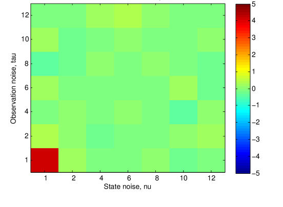
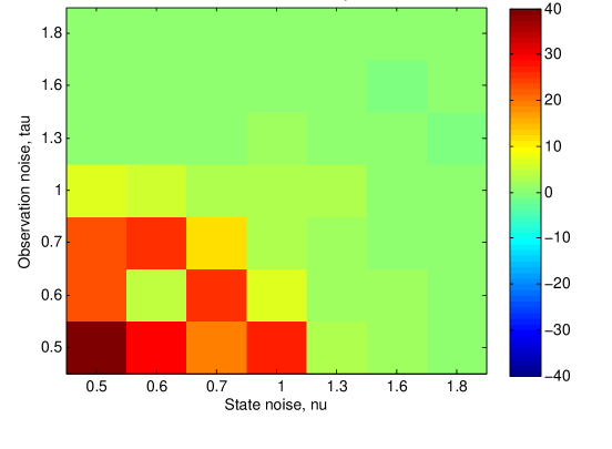
In our analysis, we calculate for different pairs of values of the state noise and the observation noise , where the variance is taken with respect to the appropriate algorithm. We run simulations per pair . The experiment is repeated under different values of for a fixed . We fix the radius of each weight, which is defined as .
The output (see Figure 7.1) is similar to the results in [23, Section 4.4]. When the noise values are concentrated around , twisting the alive particle filter results in a significant increase in the precision of . We see less of an improvement when and increase, as these are cases where the alive particle filter already performs poorly (at least under the settings that we tested).
8. Alive twisted particle marginal Metropolis-Hastings
Up to this point, the discussion has focused on sampling from (3.4). Suppose now that the model parameter is unknown, in which case we would sample from
| (8.1) |
a density which is similar to (3.3). The particle marginal Metropolis-Hastings algorithm [2] is designed for sampling from densities of the forms (3.3) and (8.1). In a particle marginal Metropolis-Hastings (PMMH) algorithm, one targets an extended density (which is henceforth denoted as ) that yields the true density of interest (or ) as a marginal; the PMMH employs SMC within a Metropolis-Hastings scheme to sample the variables of the extended target , and the acceptance ratio of that Metropolis-Hastings scheme is calculated using .
The original alive particle filter paper [13] outlines a PMMH algorithm that employs Algorithm 3, thereby allowing one to sample from (8.1). However, Section 7 shows that Algorithm 4 can indeed outperform Algorithm 3 in certain scenarios, with the variance of being reduced. In [2], the authors explain that the variance of is critical in the performance of PMMH. Thus, it is sensible to embed the alive twisted particle filter in PMMH to attempt to expedite the convergence of PMMH. As is variable, performance improvements in even just some locations of can be desirable for a PMMH.
It is straightforward to define an alive twisted PMMH as Algorithm 5, whose extended target density is structured as follows. The joint density of the simulated variables through time of Algorithm 4 is
where we use to denote the full ancestry of the twisted and non-twisted particles (note also that is being used to denote the index of the twisted particle at any time step ). One can use this expression to establish an extended target as
| (8.2) | ||||
where is an appropriate prior for the parameter . In both of the above expressions, it is assumed that, at any time step , each sample satisfies the following: . Similarly, the proposal density of the PMMH takes the form
where is the density that proposes a new value conditional on a current accepted value .
-
•
Step 0: Set arbitrarily. All remaining random variables can be sampled from their full conditionals defined by the target (8.2):
- Sample via Algorithm 4 using parameter value .
- Choose with probability .
Finally, calculate the marginal likelihood estimate, , via (5.2).
-
•
Step 1: Sample . All remaining random variables can be sampled from their full conditionals defined by the target (8.2):
- Sample via Algorithm 4 using parameter value .
- Choose with probability .
Finally, calculate the marginal likelihood estimate, , via (5.2).
-
•
Step 2: With acceptance probability
set , , , , and .
Return to the beginning of Step 1.
9. Implementation of alive twisted PMMH
In the next numerical illustration, we compare the convergence of Algorithm 5 to that of the PMMH employing the non-twisted alive particle filter (see [13]). We consider a stochastic volatility model which is similar to the one appearing in [13]:
for . This model is more challenging than the linear Gaussian HMM (7.1) because the probability density functions of the observations are not defined for all parameter values of the stable distribution. However, the stable distribution is Gaussian when the stability parameter is . Thus, this section uses the same approximation for that was used in Section 7, and only when calculating
| (9.1) |
we assume that the density of the observations is Gaussian.
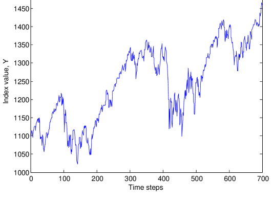
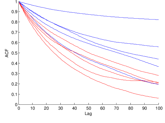
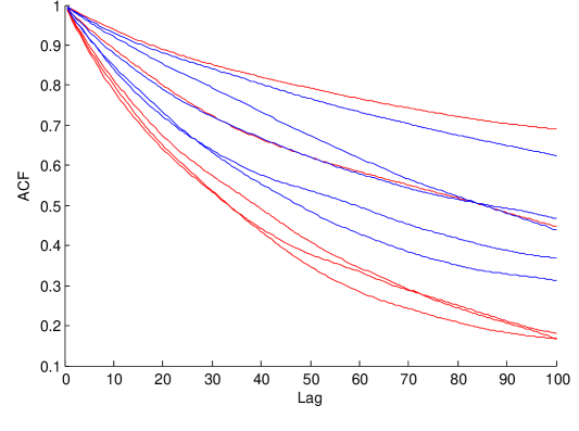
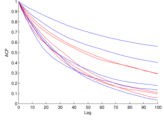
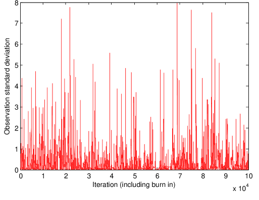
The observations are daily logarithmic returns of the S&P 500. We consider three datasets that each begin with 10th December 2009 and run for , , or time steps (see Figure 9.1). The datasets are chosen for their different time lengths, to study how affects the relative performance of the algorithms.
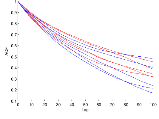
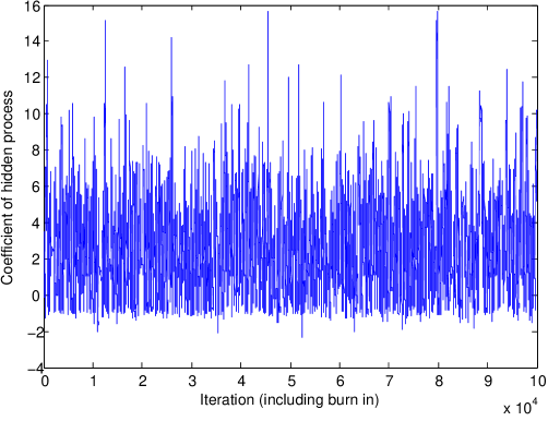
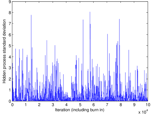
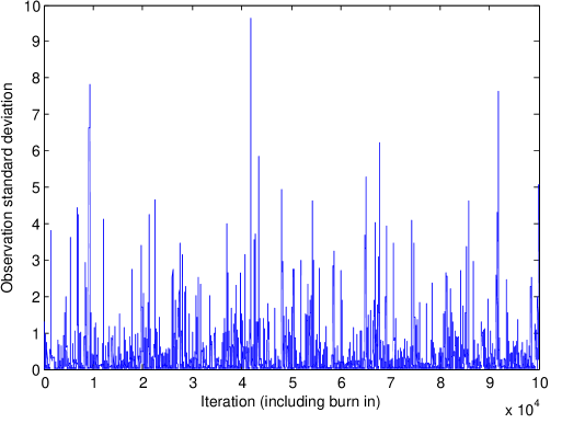
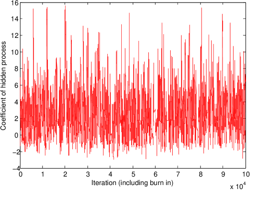
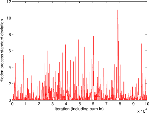
Both PMMH algorithms are used to infer the scalars , , and . We try different algorithmic settings for each of the three datasets, choosing and ; both PMMH schemes have approximately equal running times for equal values of . Across all datasets, we fix the number of PMMH iterations to , and we fix . Five runs of both algorithms are repeated per group of algorithmic settings. The proposals for the parameters and are log normal random walks: , . The proposal for is a normal random walk: . We track the convergence of the PMMH algorithms using the autocorrelation functions (ACFs) and the trace plots of , , and .
Both algorithms seem to perform similarly when , regardless of the values of or (results not shown). This output suggests that (9.1) is a poor approximation of the true eigenfunction in the case where . However, when , the ACF plots (see Figure 9.2) show the alive twisted PMMH slightly outperforming the non-twisted alive PMMH. Thus, it appears (9.1) is a fair approximation to the true, optimal when . We only present the output for (see Figures 9.2 and 9.3), as the results are similar for the slightly different values of and .
10. Discussion
In this paper, we introduced a change of measure on the alive particle filter of [13] to reduce the variance of its estimate of the normalising constant. By adopting similar assumptions as in [23], we followed the theoretical framework developed in [23] to determine the unique, optimal change of measure for the alive algorithm. That optimal choice also happens to be the same unique choice discovered in [23], which, unlike this paper, does not consider HMMs whose observations have unknown or intractable likelihood densities.
We used our theoretical findings to formalise an alive twisted particle filter and an alive twisted PMMH. Both methods were implemented on HMMs, with the PMMH being used in a real world example. The numerical analyses illustrated that when the change of measure on the alive algorithms is not a close approximation of the ideal change in measure, twisting may not be worthwhile. However, when a good approximation of the ideal change in measure was available, our algorithms did exhibit superior performance in some scenarios.
The assumptions used to prove our theoretical results may be difficult to verify. Assumption (B(B1)), in particular, would be very hard to verify when one knows little about the process producing the observations. A future work might consider proving the same results under weaker assumptions, although that will likely not be a straightforward task. Additionally, other future work might investigate possible applications outside of HMMs, such as in the rare events literature [4] or ABC approximations of epidemiological models [9].
Acknowledgment The first author was partially supported through a Roth Studentship at Imperial College London. Both authors were also supported by an MOE Singapore grant.
Appendix
A. Proof of the main result from Section 6
We first illustrate that is actually finite in the limit as , for otherwise there would be no circumstance under which . The result is established as the following proposition.
Proposition A.1.
Proof of Proposition A.1.
This proof closely follows the proof of [23, Proposition 1], with only some minor modifications. Assuming (B(B2)), we can define a constant which also must be finite. Consider a sequence of random variables where . We know , and as
we have
| (A.1) |
Furthermore, (B(B2)) and the definition of ensure that each is finite, and so
| (A.2) |
Considering (A.1), (A.2), and the ergodicity of the shift operator assumed by (B(B1)), we can apply Kingman’s subbadditive ergodic theory [16] to obtain
| (A.3) |
as , almost surely, where is a finite constant.
The next two propositions clearly define the triple that uniquely satisfies the system of equations (6.1). It is not yet shown that is the optimal measure by which Algorithm 4 should be twisted. Before proving that, we have to first show that the measure exists. The fact that the triple uniquely satisfies (6.1) is used in calculations in later parts of the proof of the main result.
Proposition A.2.
Assume (B(B2)).
-
1.
Fixing , the limits
exist, where is a member of a family of probability measures, , and is a member of a family of real-valued, measurable functions, .
-
2.
The families of probability measures and measurable functions just defined are independent of , and there exist constants and such that and
for and .
-
3.
The function is measurable, and
-
4.
Consider the triples that consist of (a) a family of probability measures on indexed by , (b) an valued measurable function on , and (c) a measurable function on . For all , the triple uniquely satisfies , , and .
Proof of Proposition A.2.
Proposition A.3.
Proof of Proposition A.3.
Now that the triple is clearly defined and it is known that is approximating a finite value in the limit as , we can begin to establish how the optimal affects the particle filter. That illustration begins by showing how the particle filter behaves when its transition density is any (which is a member of ) and not necessarily one twisted with .
The functions and of Definition 2.1 can be used to construct (2.3). Thus, for any , we establish bounds on those functions via Lemmas A.3 and A.4 below to show that , almost surely, in Proposition A.4 below.
Proof of Lemma A.3.
Under (B(B3)), it is clear that any is positive and finite, and so a positive and finite upper bound on is obvious.
Lemma A.4.
Proof of Lemma A.4.
Proposition A.4.
Proof of Proposition A.4.
Next, assume (B(B3)) and consider the bounds presented in Lemma A.4. Following the exact same steps as in the proof of [23, Proposition 1], one can show that there exists a constant such that approaches as , almost surely.
By the definition (2.3), we have , and so . ∎
There is one final lemma which is needed to prove Theorem 6.2. The following is a technical result establishing that an additive functional of the form (2.4), with optimal as defined in Proposition A.2, is an eigenfunction for .
Finally, we use the optimal of Proposition A.2 and prove that the specific, unique defined in Theorem 6.2 achieves . The main result is presented as Theorem 6.2 in Section 6, and its proof follows the same steps as in the proof of [23, Theorem 1].
B. Tables
| Distribution | Parameters | Notation | Expected value |
|---|---|---|---|
| Gamma | shape and scale | ||
| Gaussian | mean and variance | ||
| Stable | stability , skewness , | when | |
| scale , and location |
References
- [1] B. D. O. Anderson and J. B. Moore. Optimal Filtering. Prentice–Hall, Englewood Cliffs, 1979.
- [2] C. Andrieu, A. Doucet, and R. Holenstein. Particle markov chain monte carlo methods (with discussion). Journal of the Royal Statistical Society: Series B, 72:269–342, 2010.
- [3] O. Cappe, E. Moulines, and T. Ryden. Inference in Hidden Markov Models. Series: Statistics. Springer, New York, 2005.
- [4] F. C’erou, P. Del Moral, T. Furon, and A. Guyader. Sequential monte carlo for rare event estimation. Statistics and Computing, 22:795–808, 2012.
- [5] S. Colella, C. Yau, J. M. Taylor, G. Mirza, H. Butler, P. Clouston, A. S. Bassett, A. Seller, C. C. Holmes, and J. Ragoussis. Quantisnp: an objective bayes hidden-markov model to detect and accurately map copy number variation using snp genotyping data. Nucleic Acids Research, 35(6):2013–2025, 2007.
- [6] D. Crisan and B. Rozovsky (editors). Handbook of Nonlinear Filtering. Oxford University Press, Oxford, 2011.
- [7] T. A. Dean, S. S. Singh, A. Jasra, and G. W. Peters. Parameter estimation for hidden markov models with intractable likelihoods. Technical Report University of Cambridge, Department of Engineering, 2010.
- [8] P. Del Moral. Feynman-Kac formulae. Genealogical and interacting particle approximations. Series: Probability and Applications. Springer-Verlag, Heidelberg, 2004.
- [9] P. Del Moral, A. Doucet, and A. Jasra. An adaptive sequential monte carlo method for approximate bayesian computation. Statistics and Computing, 22:1223–1237, 2012.
- [10] A. Doucet, S. Godsill, and C. Andrieu. On sequential monte carlo sampling methods for bayesian filtering. Statistics and Computing, 10:197–208, 2000.
- [11] N. J. Gordon, D. J. Salmond, and A. F. M. Smith. Novel approach to nonlinear/non-gaussian bayesian state estimation. IEE-Proceedings-F, 140:107–113, 1993.
- [12] J. Hu, M. K. Brown, and W. Turin. Hmm based online handwriting recognition. IEEE Transactions on Pattern Analysis and Machine Intelligence, 18(10):1039–1045, 1996.
- [13] A. Jasra, A. Lee, C. Yau, and X. Zhang. The alive particle filter. preprint. (arXiv:1304.0151v1 [stat.CO]), 2013.
- [14] A. Jasra, S. S. Singh, J. S. Martin, and E. McCoy. Filtering via approximate bayesian computation. Statistics and Computing, 22(6):1223–1237, 2012.
- [15] S. J. Julier and J. K. Uhlmann. Unscented filtering and nonlinear estimation. Proceedings of the IEEE, 92(3):401–422, 2004.
- [16] J. F. C. Kingman. Subadditive ergodic theory. Annals of Probability, 1(6):883–909, 1976.
- [17] R. Langrock, I. L. MacDonald, and W. Zucchini. Some nonstandard stochastic volatility models and their estimation using structured hidden markov models. Journal of Empirical Finance, 19(1):147–161, 2012.
- [18] J. S. Martin, A. Jasra, S. S. Singh, N. Whiteley, and E. McCoy. Approximate bayesian computation for smoothing. preprint. (arXiv:1206.5208v1 [stat.CO]), 2012.
- [19] L. Peshkin and M. S. Gelfand. Segmentation of yeast dna using hidden markov models. Bioinformatics, 15(12):980–986, 1999.
- [20] R. A. Rosales, M. Fill, and A. L. Escobar. Calcium regulation of single ryanodine receptor channel gating analyzed using hmm/mcmc statistical methods. Journal of General Physiology, 123:533–553, 2004.
- [21] N. Shephard and M. K. Pitt. Likelihood analysis of non-gaussian measurement time series. Biometrika, 84(3):653–667, 1997.
- [22] S. Tavare, D. J. Balding, R. C. Griffiths, and P. Donnelly. Inferring coalescence times from dna sequence data. Genetics, 145:505–518, 1997.
- [23] N. Whiteley and A. Lee. Twisted particle filters. preprint. http://www.maths.bris.ac.uk/~manpw/, 2013.
- [24] C. Yau, O. Papaspiliopoulos, G. O. Roberts, and C. C. Holmes. Bayesian non-parametric hidden markov models with applications in genomics. Journal of the Royal Statistical Society: Series B, 73(1):33–57, 2011.
Department of Mathematics, Imperial College London, London, SW7 2AZ, UK. E-mail: a.persing11@ic.ac.uk
Department of Statistics & Applied Probability, National University of Singapore, Singapore, 117546, SG. E-mail: staja@nus.edu.sg