A Numerical Test of Pade Approximation for Some Functions with singularity

Abstract

The aim of this study is to examine some numerical tests of Pade approximation for some typical functions with singularities such as simple pole, essential singularity, brunch cut and natural boundary. As pointed out by Baker, it was shown that the simple pole and the essential singularity can be specified by the poles of the Pade approximation. However, it have not necessarily been clear how the Pade approximation work for the functions with the branch cut or the natural boundary. In the present paper, it is shown that the poles and zeros of the Pade approximated functions are alternately lined along the branch cut if the test function has branch cut, and poles are also distributed around the natural boundary for some lacunary power series and random power series which rigorously has a natural boundary on the unit circle. On the other hand, spurious poles and zeros (Froissart doublets) due to numerical errors and/or external noise also appear around the unit circle in the Pade approximation. It is also shown that the residue calculus for the Pade approximated functions can be used to confirm the numerical accuracy of the Pade approximation and quasianalyticity of the random power series.

I Introduction

Pade approximation was introduced in Mathematics and it has been used in Physics for more than 40 years ago baker70 ; baker75 ; baker96 . In particular, there have been several important examples in Physics, to which Pade approximation was applied, such as summation of the divergent Rayleigh-Schrodinger perturbation series in scattering theory sasagawa81 , critical phenomena in statistical physics stanly71 ; yang52 ; nickel99 ; kubo85 ; macoy01 , denoising from noisy data of time-series, bessis96 ; stahl97 ; gilewicz97 ; bessis09 ; antonio09 , detection of singularity of phase space trajectories of Hamiltonian dynamical systems berrretti90 ; falcolini92 ; llave94b ; berretti95 ; berretti01 , and so on.

Mathematically, the Pade approximation is used to estimate analyticity of functions. Indeed, the Pade approximation is usually superior to the truncated Taylor expansions when the original function contains any singularity. Let us consider a simple example. The function $f(z)=\sqrt{\frac{1+2z}{1+z}}$ has brunch points at $z=-1$ and $z=-1/2$. The domain of convergence is $|z|<1/2$. Nevertheless, we can obtain an exact solution $\surd 2=1.4142$ for $z\to\infty$ when we apply $[3|3]$ diagonal Pade approximation to the function. (See Sect. III.3 for more details of this example.) Although the mathematical validity of Pade approximation has not been exactly proved yet, The Pade approximation is practically very useful to continue a singular function beyond the the domain of convergence.

Let us consider a critical phenomenon for Ising model as a simple example in statistical Physics stanly71 ; kubo85 ; nickel99 . We assume that at the critical point $u=u_{c}$ the exact magnetic susceptibility $\chi$ has a singularity as

$$\chi\sim(u-u_{c})^{-\gamma},$$ (1)

where $u$ is a function of temperature and interactions and so on. In this case we sometimes use the logarithmic derivative of $\chi$ when we estimate the critical point $u=u_{c}$ and the critical exponent $\gamma$ as a pole-type singularity as,

$$\frac{d\log\chi}{du}=\frac{\chi^{{}^{\prime}}}{\chi}=\frac{\gamma}{(u-u_{c})},$$ (2)

where $\chi^{{}^{\prime}}$ denotes the derivative with respect to the variable $u$. In the low temperature expansion for the magnetic susceptibility $\chi$ with some coefficients ${a_{n}}$, we assume that the approximated susceptibility $\chi_{N}$ and the logarithmic derivative are obtained as follows,

$$\chi\sim\chi_{N}=\sum_{n=0}^{N}a_{n}u^{n},~{}~{}~{}\frac{\chi^{{}^{\prime}}}{\chi}\sim\sum_{n=0}^{N}b_{n}u^{n}.$$ (3)

Then we can estimate the critical point $u=u_{c}$ and the critical exponent $\gamma$ applying the Pade approximation to the truncated expansion $\chi_{N}$. Note that the singularity on $|u|=u_{c}$ will be infinitely differentiable if the coefficients $a_{n}$ fall off sufficiently rapidly.

In general, analytic continuation over the singular point is possible along any other path in complex plane even if the function diverges at the singular point determining the radius of convergence, as seen in the above singularity of the Ising model. Therefore, the Pade approximation is useful to improve the convergence of the power series and approximate the exact solution.

Furthermore, the Pade approximation has been used to investigate convergence of Fourier series baker75 ; baker96 and the breakdown of KAM curves in complex plane for Hamiltonian map systems, which is described as the analytic domains of Lindstedt series for standard map berrretti90 ; falcolini92 ; llave94b ; berretti95 ; berretti01 .

In addition, we can see an interesting example concerning the Pade approximation in noisy data analysis bessis96 ; stahl97 ; gilewicz97 ; bessis09 ; antonio09 . The power series with finite random coefficient “almost always” has a natural boundary on the unit circle in the complex plane korner93 ; remmert10 ; breuer11 ; knill10 ; costin . In a finite time-series, Froissart has shown that a natural boundary generated by the random time-series is approximated by doublets of poles and zeros (Froissart doublets) of the Pade approximated function surrounding the vicinity of the unit circle. Taking advantage of the characteristic, the Pade approximation has been used in order to remove the noise and extract the true poles associated with damping modes from the observed noisy time-series.

The main purpose of the present paper is to investigate whether the Pade approximation is numerically useful for detecting the singularity of some test functions. In particular, we examine the usefulness for the functions with a natural boundary such as a lacunary power series and a random power series baker75 ; berretti95 ; bessis09 .

The organization of the paper is the following: In Sect.II, we give a brief explanation of the Pade approximation and some important reminders in the numerical calculation. In Sect.III, we present some numerical results of the Pade approximation for test functions with branch cut, essential singularity. We also try to apply the Pade approximation to an entire function. In Sect.IV, application of the Pade approximation to some lacunary series which is known to have a natural boundary is given. In Sect.V, numerical results of the application to random power series with a natural boundary and some test functions with random noise are also shown. In Sect.VI, we discuss about the residue calculus for the Pade approximated functions to confirm the numerical errors and quasianalyticity of the random power series. In the last section, we give summary and discussion.

In appendix A, the general result for Fibonacci generator used in the Subsect.III.2 is given. In appendix B, some theorems concerning zeros of polynomials are given. In appendix C, some mathematical theorems for lacunary series which are useful in reading the main text, are summarized. In appendix D, exact Pade approximated function to some lacunary power series with a natural boundary are given. Residue analysis for quasianalytic functions of Carleman class is given in the appendix E. Furthermore, some theorems concerning the random power series are given in appendix F.

II Pade approximation

For a given function $f(z)$, a truncated Taylor expansion $f^{[N]}(z)$ of order $N$ about zero is given as,

$$f(z)\sim f^{[N]}(z)=\sum_{n=0}^{N}c_{n}z^{n},$$ (4)

where ${c_{n}}$ denotes the coefficients of the Taylor expansion. Pade approximation is more accurate approximations for $f(z)$ up to order $O(z^{N})$ than the Taylor expansion. The Pade approximation is a rational function, viz. a ratio of two polynomials, which agrees to the highest possible order $O(z^{N})$ with a truncated polynomial $f^{[N]}(z)$ as follows.

$$f^{[N]}(z) = \frac{a_{0}+a_{1}z+a_{2}z^{2}+....a_{L}z^{L}}{1+b_{1}z+b_{2}z^{2}+.......b_{M}z^{M}}$$ (5)

$$\equiv \frac{P_{L}(z)}{Q_{M}(z)}\equiv f^{[L|M]}(z),$$ (6)

where $P_{L}(z)$ is a polynomial of degree less than or equal to $L$ and $Q_{M}(z)$ is a polynomial of degree less than or equal to $M$. Note that $b_{0}=1$ (normalized) here. A unique approximation can be specified for all choice of $M$ and $L$ such that $N=L+M$ when it exists. The coefficients $\{a_{n}\},\{b_{n}\}$ can be obtained from the condition that the first $(L+M+1)$ terms vanish in the Taylor series. The difference between the Pade approximation and the original function satisfies a following equation,

$$f(z)-f^{[L|M]}(z)=O(z^{L+M+1}).$$ (7)

In this paper, we sometimes use ”$[L|M]$ Pade approximation” or ”$[L|M]$ Pade approximated function” for $f^{[L|M]}(z)$. Solving the problem in Eq.(7) is called a linear Teoplitze problem which is generally ill-conditioned. We used full LU decomposition for the Teoplitze matrix in the problem as well as iterative improvement in order to eliminate the ill-posed problem press88 . In addition, hereafter, we use the diagonal Pade approximation, i.e. $L=M$, of order $M\leq 65$ to estimate the singularity of the test functions because of the convergence and limitation due to the round-off errors and other source of numerical errors. Here, the singularity of the function $f(z)$ is approximated by configuration of the poles and zeros of the $[M|M]$ order diagonal Pade approximated function. As mentioned in introduction, in general, Pade approximations are useful for representing unknown functions with possible poles. The application of the diagonal Pade approximation is insured for the functions with isolated singular points and rational-type functions. However, it is not fully-clarified that how the poles and zeros of the Pade approximated function describe essential singularity, brunch cut and natural boundary.

Generally, the magnitude of the residues associated with the spurious poles are much smaller than those with the true poles, and they are close to machine precision. Very recently, Gonnet et al. suggested an efficient algorithm for the Pade approximations gonnet11 ; gonnet12 . The algorithm detects and eliminates the spurious pole-zero pairs caused by the rounding errors by means of singular value decomposition for the Teoplize matrix.

Before closing this section, we list up some important reminders when we numerically apply the Pade approximation to unknown functions.

1. More accurate calculation becomes possible by a scaling the expansion variable $z$ if there is a simple pole with large magnitude $\rho$($>>1$). That is, we should change the order of radius of convergence into $O(1)$ by the scaling the expansion variable as $z\to z/\rho$ in order to keep the numerical accuracy. This procedure is effective when we apply the Pade approximation to exponentially decaying coefficients $\{a_{n}\}$ with fluctuation.

2. Poles (i.e. roots of $P_{M}(z)=0$ ) and zeros (i.e. roots of $Q_{M}(z)=0$) are sometime cancelled (zero-pole ghost pairs). We can remove the effects of the ghost pairs and confirm the singularity of the functions by using the residue analysis of the Pade approximated function.

3. Poles and zeros of the Pade approximation to the truncated random power series accumulate around the unit circle as Froissart doublets. It is difficult to distinguish whether the poles of the Pade approximation originated from a natural boundary of the original function or the natural boundary generated by the numerical error and/or noise. Therefore, the numerical accuracy will be important to determine the coefficients of the Pade approximation.

4. In general, the denominators of the diagonal Pade approximated functions to the lacunary power series and the random power series become lacunary and random polynomials, respectively. Accordingly, the distribution of the poles and zeros of the approximated functions are similar to the distribution of the zeros corresponding to the original lacunary power polynomial and random power polynomial. In particular, it is well-known that the zeros of the random polynomials uniformly distribute about the unit circle.

III Examples of Pade Approximation for Some Functions

In this section we investigate the configuration of the poles and zeros of the Pade approximation to some test functions with singularity.

III.1 comparison of Pade approximation with Taylor expansion

First, we try the Pade approximation to the following test function $f_{1}(z)$ with a brunch point at $z=-1$,

$$f_{1}(z) = \frac{\log(1+z)}{z}.$$ (8)

The truncated Taylor expansion of the order $N=4$ around $z=0$ is

$$f_{1}^{[4]}(z) = 1-\frac{1}{2}z+\frac{1}{3}z^{2}-\frac{1}{4}z^{3}+\frac{1}{5}z^{4}.$$ (9)

The $[2|2]$ Pade approximation is given as,

$$f_{1}^{[2|2]}(z) = \frac{1+\frac{7}{10}z+\frac{1}{30}z^{2}}{1+\frac{6}{5}z+\frac{3}{10}z^{2}}.$$ (10)

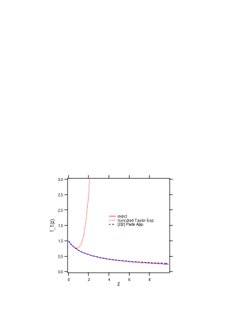
Figure 1 shows the approximated functions the truncated Taylor series $f_{1}^{[4]}(z)$ and the original test function $f_{1}(z)$. The approximated function $f_{1}^{[4]}(z)$ by the truncated Taylor expansion converges only within $|z|<1$ and deviates from the exact function $f_{1}(z)$ for $|z|>1$. On the other hand, it follows that the Pade approximated function $f_{1}^{[2|2]}(z)$ well-approximates the original function $f_{1}(z)$ with very high precession even beyond the radius of convergence up to $Rez=x\sim 10$. Therefore, it is found that the divergent power series expansion (Taylor expansion) does still contain information about the original function outside the convergence radius, and rearranging the coefficients of the expansion into the Pade approximation recovers the information. As a result, the conversion from the Taylor-form to the Pade-form usually accelerates the convergence and often allows good accuracy even outside the radius of convergence of the power series.

Figure 1: (Color online) The Pade approximated function $f_{1}^{[2|2]}(z)$, the truncated Taylor series $f_{1}^{[4]}(z)$ and the original test function $f_{1}(z)$.

III.2 Pade approximation for Fibonacci generating function

Let us consider the Fibonacci generating function $f_{F}(z)$, where Fibonacci sequence $\{F_{n}\}$ is encoded in the power series as the coefficients. The Fibonacci sequence $\{F_{n}\}$ is given by the following recursion relation:

$$F_{n}=F_{n-1}+F_{n-2}(n\geq 2),$$ (11)

where $F_{0}=0$ and $F_{1}=1$. Then the Fibonacci generating function $f_{F}(z)$ becomes

$$f_{F}(z) = \sum_{n=0}^{\infty}F_{n}z^{n}$$ (12)

$$= \frac{z}{1-z-z^{2}}$$ (13)

$$= \frac{1}{\sqrt{5}}\frac{1}{1-\phi^{+}z}-\frac{1}{\sqrt{5}}\frac{1}{1-\phi^{-}z},$$ (14)

where $\phi^{+}\equiv\frac{1+\sqrt{5}}{2}(=1.61803.....)$ and $\phi^{-}\equiv\frac{1-\sqrt{5}}{2}(=-0.61803...)$. The generating function has poles at $z=\phi^{+}$ and $z=\phi^{-}$. Generating functions by more general recursion relation is given in appendix A.

It should be noted that the diagonal Pade approximation $f_{F}^{[\frac{N}{2}|\frac{N}{2}]}(z)$ for the truncated Fibonacci generation function $f_{F}^{[N]}(z)=\sum_{n=0}^{N}F_{n}z^{n}$ has the form

$$f_{F}^{[\frac{N}{2}|\frac{N}{2}]}(z)=\frac{z}{1-z-z^{2}}+O(z^{N+1}),$$ (15)

for even number $N\geq 2$. This means that the diagonal Pade approximation can detect the exact poles of the generating function irrespective of the order.

III.3 Examples of some test functions with pole, brunch cut and essential singularity

In this subsection, we use some test functions in applying of the Pade approximation.

$$f_{2}(z) = e^{-z},$$ (16)

$$f_{3}(z) = \sqrt{\frac{1+2z}{1+z}},$$ (17)

$$f_{4}(z) = e^{-z/(1+z)},$$ (18)

$$f_{5}(z) = \tan z^{4}.$$ (19)

Here, $f_{2}(z)$ has no singularity for $|z|<\infty$, $f_{3}(z)$ has a brunch cut along a line on $[-1,-1/2]$, and $f_{4}(z)$ has an essential singularity at $z=-1$. $f_{5}(z)$ has eight poles at points on the unit circle $z={\rm exp}\{i\pi\frac{m}{4}\}(m=0,1,2,...,7)$.

First, let us apply Pade approximation to $f_{2}(z)$. In this case the explicit form of the Pade approximated function can be obtained in the following form,

$$P_{M}(z) = \sum_{k=0}^{M}\frac{(2M-k)!M!}{(2M)!k!(M-k)!}(-z)^{k},$$ (20)

$$Q_{M}(z) = \sum_{k=0}^{M}\frac{(2M-k)!M!}{(2M)!k!(M-k)!}z^{k}.$$ (21)

Note that the coefficients of the numerator $P_{M}(z)$ have always alternatively sign, and the zeros and poles of Pade approximated function are symmetrical to the imaginary axis with each other because $P_{M}(z)=Q_{M}(-z)$. Figure 2(a) shows the numerical results in the complex $z-$plane. All poles are on the left-half plane $Rez>0$, and all zeros are on the right-half plane $Rez<0$. The poles and zeros of the Pade approximated functions for the regular function $f_{2}(z)$ go infinity and disappear as $M\to\infty$ because the function $f_{2}(z)$ is an entire function.

Figure 2: (Color online) Distributions of poles ($\bullet,\bigcirc$) and zeros ($+,\times$) of the $[M|M]$ diagonal Pade approximated functions to some test functions:(a)$f_{2}(z)$, (b)$f_{3}(z)$, (c)$f_{4}(z)$.

Figure 3: (Color online) Distributions of poles ($\bigcirc$) and zeros ($\times$) of the $[M|M]$ diagonal Pade approximated functions to the test function $f_{5}(z)$. (a)The $[50|50]$ Pade approximation. (b)The $[75|75]$ Pade approximation. The unit circle is drawn to guide the eye.

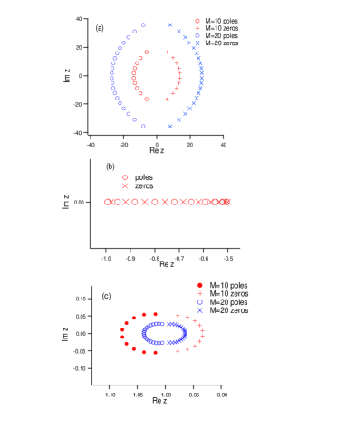
In Fig.2(b), distribution of the zeros and poles of Pade approximated function to $f_{3}(z)$ are shown. The poles and zeros make a line alternately between the two branch points of the $f_{3}(z)$; $z=-1$ and $z=-1/2$.

Figure 2(c) shows the distribution of the zeros and poles of the Pade approximation to $f_{4}(z)$. Pade approximation clusters the poles and zeros at the singular point for $f_{4}(z)$. As $M\to\infty$ the poles and zeros approach the singular point $z=-1$ that reflects the essential singularity of the original function $f_{4}(z)$.

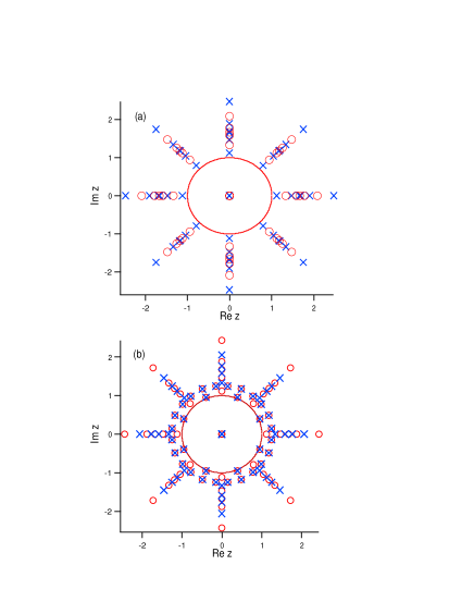
Figure 3(a) shows the poles and zeros of the Pade approximated function to the test function $f_{5}(z)$. The poles and zeros are alternatively distributed in eight-direction from the origin. It seems that the distance between the poles and/or zeros on the same line becomes small as they approach the location of the true poles. Some ”spurious poles” appear around the unit circle as increase of the order of the Pade approximation, as seen in Fig.3(b), which are irrelevant poles due to insufficient numerical accuracy. It is found that the numerical accuracy of the Pade approximation fails for the higher order of the Pade approximation. We discuss about the spurious poles in Sect.IV and V again.

IV natural boundary of lacunary power series

In this section we examine the applicability of the Pade approximation to investigating the analyticity of some well-known test functions with a natural boundary on the unit circle $|z|=1$. This will provide a preliminary information about what occurs in the Pade approximated functions with a natural boundary. Indeed, we do know only a very few numerical examples which has a natural boundary and allows an exact diagonal Pade approximation.

There are following famous lacunary power series with a natural boundary on the unit circle $|z|=1$, $f_{Jac}(z)=\sum_{n=0}^{\infty}z^{2^{n}}$, $f_{Wie}(z)=\sum_{n=0}^{\infty}z^{n!}$, $f_{Kro}(z)=\sum_{n=0}^{\infty}z^{n^{2}}$, where the $f_{Jac}(z)$, $f_{Wie}(z)$ and $f_{Kro}(z)$ are called after Jacobi, Weierstrass and Kronecker. Some theorems for the lacunary series with a natural boundary are given in appendix C korner93 ; remmert10 ; breuer11 .

Here, we use polar-form $f_{r}(\theta)$ for the function $f(z)$ by changing the variable, i.e. $z=re^{i\theta}$, in order to simply display the functions as;

$$f_{r}(\theta)=f(z=re^{i\theta})=\sum_{n=0}^{\infty}c_{n}(re^{i\theta})^{n}.$$ (22)

Then, note that the modulus $r$ works as a convergence factor of the series because it well converges for $r<1$. Typically we take $r=1$ on the unit circle or $r=0.98$ inside the circle in the following numerical calculations.

IV.1 Example 1: Jacobi lacunary series

We try to apply Pade approximation to the function $f_{Jac}(z)$ with a natural boundary on the unit circle $|z|=1$. The Pade approximated function exactly has the following form,

$$f^{[2^{N}]}_{Jac}(z) \sim f_{Jac}^{[2^{N-1}|2^{N-1}]}(z)$$ (23)

$$= \frac{A^{N}_{Jac}(z)}{1+\sum_{k=0}^{N-2}z^{2^{k}}-z^{2^{N-1}}},$$ (24)

where the explicit form of the numerator $A^{N}_{Jac}(z)$ is given in appendix D. Accordingly, the poles of the $[2^{N-1}|2^{N-1}]$ Pade approximated function is given by roots of the polynomial,

$$1+\sum_{k=0}^{N-2}z^{2^{k}}-z^{2^{N-1}}=0.$$ (25)

This is also just a lacunary polynomial. In Fig.4 the numerical result of the Pade approximation for $f_{Jac}(z)$ is shown. The poles and zeros are plotted for the $[64|64]$ Pade approximation in Fig.4(a). Inside the circle $|z|=1$ some cancellations of the ghost pairs appear. The poles and zeros accumulate around $|z|=1$ as increase of order of the Pade approximation. In the case of the $M=64$, the poles accumulate around $|z|=1$ with making the zero-pole pairings. Figure 4(b) shows the Pade approximated functions in the polar-form with $r=1$. It well approximate the original function $f_{Jac}(z)$ when the order of the Pade approximation increases.

Figure 4: (Color online) (a)Distribution of poles($\bigcirc$) and zeros($\times$) of the $[64|64]$ Pade approximation to the test function $f_{Jac}(z)$ with a natural boundary on $|z|=1$. The unit circle is drawn to guide the eye. (b)The Pade approximated functions $f_{Jac}^{[32|32]}(\theta)$, $f_{Jac}^{[64|64]}(\theta)$ and the exact function $f_{Jac}(\theta)$ in the polar-form with $r=1.0$. (After Ref.yamada13 .)

It is also shown that the complex zeros of the polynomial (25) cluster near unit circle $|z|=1$ and distribute uniformly on the circle as $F_{N}\to\infty$ by Erdos-Turan type theorem given in appendix C and B kac43 ; erdos50 ; amoroso96 ; odlyzko93 ; simon04a ; simon04b ; peres05 ; simon10 .

IV.2 Example 2: Fibonacci lacunary series

As a second example, we would like to apply Pade approximation to the following lacunary series

$$f_{Fib}(z)=\sum_{n=0}^{\infty}z^{F_{n}},$$ (26)

where $F_{n}$ is $n$th Fibonacci number. This function also has a natural boundary on $|z|=1$. The Pade approximated function exactly has following form,

$$f^{[F_{N}]}_{Fib}(z) \sim f^{[\frac{F_{N}}{2}|\frac{F_{N}}{2}]}_{Fib}(z)$$ (27)

$$= \frac{A^{F_{N}}_{Fib}(z)}{1+z^{F_{N-4}}-z^{F_{N-2}}}.$$ (28)

The explicit form of the numerator $A^{F_{N}}_{Fib}(z)$ is given in appendix D. The poles of the $[\frac{F_{N}}{2}|\frac{F_{N}}{2}]$ Pade approximated function is given by zeros of the lacunary polynomial,

$$1+z^{F_{N-4}}-z^{F_{N-2}}=0.$$ (29)

In Fig.5 the numerical result of the Pade approximation to $f_{Fib}(z)$ is shown. The poles and zeros are plotted for the $[55|55]$ Pade approximation in Fig.5(a). The poles and zeros accumulate around $|z|=1$ as increase of the order of the Pade approximation. No pole appears inside the unit circle. The original function is also well approximated by the $[56|56]$ Pade approximation. (See Fig.5(b).)

Figure 5: (Color online) (a) Distribution of poles ($\bigcirc$) and zeros ($+$) of the $[55|55]$ Pade approximated function to the test function $f_{Fib}(z)$ with a natural boundary on $|z|=1$. The unit circle is drawn to guide the eye. (b)The Pade approximated functions $f_{Fib}^{[21|21]}(\theta)$, $f_{Fib}^{[34|34]}(\theta)$, $f_{Fib}^{[55|55]}(\theta)$ corresponding to $N=F_{9}=55$, $N=F_{10}=89$, $N=F_{11}=144$, respectively, and the exact function $f_{Fib}(\theta)$ in the polar-form with $r=1.0$. (After Ref.yamada13 .)

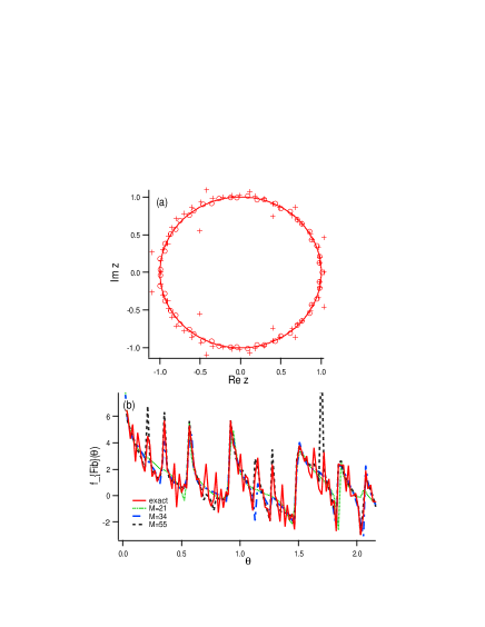
V Natural boundary of random power series and the noise-effect on Pade approximation

In this section, we apply Pade Approximation to the random power series with a natural boundary with probability 1, and investigate how the approximation detect the singularity of the series. In addition, we examine effect of noise on the coefficients of the power expansion for some test functions. Some related theorems for the natural boundary of the function generated by the random power series are given in appendix F.

V.1 Random power series and natural boundary

Let us consider a random power series,

$$f_{noise1}(z) = \sum_{n=0}^{\infty}\epsilon r_{n}z^{n}.$$ (30)

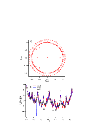
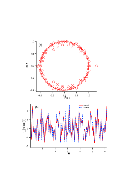
Here the sequence $r_{n}$ is $n-$independent random variable which take a value within $r_{n}\in[0,1]$, and $\epsilon$ is the strength of the randomness. It is shown that, in general, the random power series has a natural boundary on the unit circle $|z|=1$ with probability one. Figure 6(a) shows distribution of poles and zeros of the $[50|50]$ Pade approximated function to $f_{noise1}(z)$. Some pairs of poles and zeros are perfectly cancelled inside the circle $|z|=1$. On the other hand, almost all the poles and zeros of the Pade approximated function assemble around the circle $|z|=1$ and not cancelled. The pair of poles and zeros around the circle $|z|=1$ is called ”Froissart doublets”, and it well correspond to the natural boundary of $f_{noise1}(z)$. The original function is also well approximated by the $[50|50]$ Pade approximation. (See Fig.6(b).)

Figure 7 shows an example of the coefficients $\{c_{n}\}=\{\epsilon r_{n}\}$ of the random power series and the coefficients $\{a_{n}\}$ and $\{b_{n}\}$ of the $[50|50]$ Pade approximated function. The fluctuation of the coefficient $\{b_{n}\}$ that determines the poles of the Pade approximated function is smaller than those of $\{a_{n}\}$ of the numerator.

Figure 6: (Color online) (a)Distribution of poles ($\bigcirc$) and zeros ($\times$) of the Pade approximated function $f_{noise1}^{[50|50]}(z)$ to a random power series $f_{noise1}(z)$ with $\epsilon=1$. The unit circle is drawn to guide the eye. (b)The Pade approximated function $f_{noise1}^{[50|50]}(\theta)$, and the exact function $f_{Fib}(\theta)$ in the polar-form with $r=1.0$.

Figure 7: (Color online) (a)The coefficient $\{c_{n}\}=\{\epsilon r_{n}\}$ of a truncated random power series $f_{noise1}^{[100]}(z)$ with $\epsilon=0.1$. (b)The coefficients $\{a_{n}\}$ and $\{b_{n}\}$ of the Pade approximated function $f_{noise1}^{[50\mid 50]}(z)$ to $f_{noise1}^{[100]}(z)$.

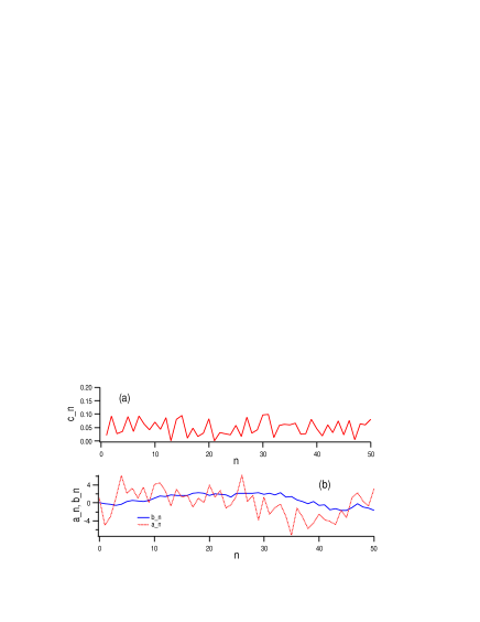
The truncated random series is just random polynomial. It is well-known that the distribution of the zeros of the random polynomials converges unit circle as increase of the order (Erdos-Turan type theorem) kac43 ; erdos50 ; peres05 . Accordingly, we can interpret that in the Pade approximated function to the random power series the distribution of poles and zeros also accumulate around the unit circle when the order of the Pade approximation increases.

V.2 Effect of noise on a function with a simple pole

In the following subsections, we investigate influences of noise on the Pade approximation for some constructed noisy test functions as follows,

$$f_{test+noise2}(z) = f_{test}(z)+f_{noise2}(z),$$ (31)

where $f_{test}(z)=\sum_{n=0}^{\infty}a_{n}z^{n}$ and $f_{noise2}(z)=\sum_{n=0}^{\infty}\epsilon_{n}z^{n}$. The $\{\epsilon_{n}\}$ is a i.i.d. random variables within $[-\epsilon,\epsilon]$ where $\epsilon$ is the noise strength. Essentially, $f_{noise2}(z)$ is the same as the random power series $f_{noise1}(z)$. First of all, in this subsection, we consider a truncated function with a simple pole. Note that if $a_{n}=C$(constant) and $\epsilon=0$, i.e., in noise-free case, $f_{pole+noise}(z)=C\sum_{n=0}^{\infty}z^{n}=\frac{C}{1-z}$ with a simple pole at $z=1$. In Ref.baker75 by Baker, the noise effect is summarized as follows: The $[M|M]$ Pade approximation has an unstable zero at the distance of order $\epsilon^{-1}$ from the origin, and the other zeros make $(M-1)$ Froissart doublets (zero-pole pairs) with the zeros.

Next, we consider a function

$$f_{pole2+noise2}(z) = f_{pole2}(z)+f_{noise2}(z),$$ (32)

$$= \sum_{n=0}^{\infty}(\frac{1}{2^{n}}+\epsilon_{n})z^{n},$$ (33)

with the noise strength $\epsilon<1$. Note that

$$f_{pole2}(z)=\frac{2}{(2-z)},$$ (34)

with a simple pole at $z=2$ to clearly show the shift of the poles of the approximated function due to the noisy series.

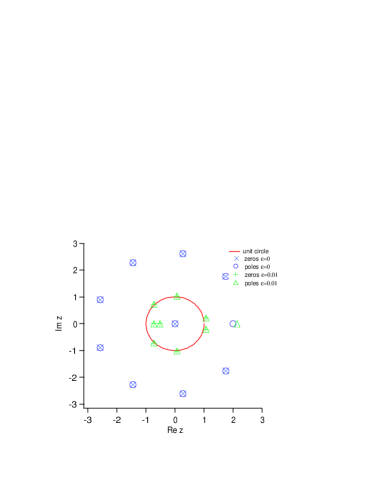
Figure 8 shows distribution of the poles and zeros of the $[10|10]$ Pade approximated functions. It clearly shows the pole-shift by the noise effect. In the noise-free case ($\epsilon=0$), a pole of the Pade approximation appears at $z=2$ and the other poles are cancelled with zeros (zero-pole ghost pairs). In a case when the relatively small noise ($\epsilon=0.01$) is added, the poles and zeros move toward $|z|=1$ with making Froissart doublets, although a pole at $z=2$ is quite stable. It becomes impossible to detect the true pole at $z=2$ when the noise strength is relatively large ($\epsilon=0.1$), not shown in the Fig.8.

As a result, it is found that the locations of the ghost pairs are unstable for noise, and the residues for the poles are much smaller than one corresponding to the true pole. We can guess that the proximity of the non-modal poles and zeros of the Pade approximated function can be understood in a sense that the poles due to the noise need zeros to cancel with each other as $\epsilon\to 0$.

Figure 8: (Color online) Distribution of poles ($\bigcirc$,$\bigtriangleup$) and zeros ($\times$,$+$) of the $[10|10]$ Pade approximated function $f_{pole2+noise2}^{[10|10]}(z)$ with a stable pole at $z=2$ for noise strength $\epsilon=0$,$\epsilon=0.01$. The unit circle is drawn to guide the eye.

V.3 Effect of noise on a function with a branch cut

We investigate the effect of the noise on functions with a branch cut. First, let us consider a function

$$f_{branch1}(z)=\sqrt{\frac{3+z}{1+z}},$$ (35)

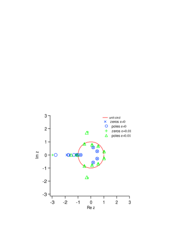
with an algebraic branch points at $z=-1$ and $z=-3$, and with the branch cut in $[-3,-1]$. Distribution of the poles and zeros of the Pade approximated function $f_{branch1+noise2}^{[10|10]}(z)$ is shown in Fig.9. In a case with relatively small noise ($\epsilon=0.01$), some poles make a line on the branch cut, and some poles and zeros move toward the unit circle $|z|=1$. It is impossible to detect the branch cut when the noise strength is relatively large ($\epsilon=0.1$).

Figure 9: (Color online) Distribution of poles ($\bigcirc$,$\bigtriangleup$) and zeros ($\times$,$+$) of the $[10|10]$ Pade approximated function $f_{branch1+noise2}^{[10|10]}(z)$ with a brunch cut from $z=-\infty$ to $z=0$ for the noise strength $\epsilon=0$,$\epsilon=0.01$. The unit circle is drawn to guide the eye.

Next, let us consider a function

$$f_{branch2}(z)=\log(\frac{6}{5}-z),$$ (36)

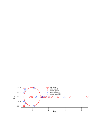
with a logarithmic branch point at $z=6/5$, and with a brunch cut from $z=6/5$ to $z=\infty$. The distribution of the poles and zeros of the Pade approximated function $f_{branch2+noise2}^{[10|10]}(z)$ for the $f_{branch2}(z)$ with the noisy perturbation is shown in Fig.10. Some poles and zeros are making a line alternatively on the branch cut in the noise-free case ($\epsilon=0$). It assemble around the unit circle $|z|=1$ with making Froissart doublets when the noise with strength $\epsilon=0.01$ is added.

Figure 10: (Color online) Distribution of poles ($\bigcirc$,$\bigtriangleup$) and zeros ($\times$,$+$) of the $[10|10]$ Pade approximated function $f_{branch2+noise2}^{[10|10]}(z)$ with a brunch cut from $z=6/5$ to $z=\infty$ for the noise strength $\epsilon=0$,$\epsilon=0.01$. The unit circle is drawn to guide the eye.

V.4 Effect of noise on a function with a natural boundary

Figure 11 shows distribution of the poles and zeros of the $[50|50]$ Pade approximated function to

$$f_{Jac+noise}(z) = f_{Jac}(z)+f_{noise2}(z),$$ (37)

which has a natural boundary on $|z|=1$.

Figure 11: (Color online) Distribution of poles ($\bullet,\bigcirc,\bigtriangleup$) and zeros ($\times+,*$) of the Pade approximated function $f_{Jac+noise}^{[50|50]}(z)$ for the lacunary series $f_{Jac+noise}^{[100]}(z)$ with a natural boundary on $|z|=1$. The noise strengths are $\epsilon=0$, $\epsilon=0.001$, $\epsilon=0.01$, respectively. The unit circle is drawn to guide the eye.

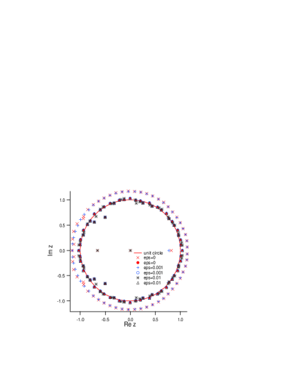
In the noise-free case, the pairs of poles and zeros of the Pade approximated function are perfectly cancelled inside the unit circle $|z|=1$. The other poles and zeros of the Pade approximated function assemble around the circle $|z|=1$ without cancellation. In the relatively small noise case ($\epsilon=0.01$), the location of the poles is not significantly changed compared with the zeros shifted outside the unit circle due to the noise effect. And, again, the poles and zeros move toward $|z|=1$ with making Froissart doublets when the noise strength is relatively large ($\epsilon=0.1$). It is closely related to a fact that fluctuation of the coefficients of the numerator of the Pade approximated function is much larger than those in the denominator, as seen in Pade approximation to the random power series in Fig.7. As a result, the singularity of the Pade approximated function to the function with a natural boundary is more sensitive to the noisy perturbation than those in the functions with the other type singularity such as simple poles and branch points.

It is very difficult to effectively distinguish whether the poles of the Pade approximation originated from the natural boundary on $|z|=1$ of the original function $f_{Jac}(z)$ or from the other natural boundary on $|z|=1$ generated by noisy series $f_{noise2}(z)$ or numerical errors. Actually the round-off error effects on the distribution of the poles and zeros of the Pade approximated function. Accordingly, to determine the expansion coefficients $c_{n}$ with adequate accuracy becomes very important in the numerical calculation. This is a drawback of the Pade approximation when we use it for functions with unknown singularities.

V.5 Numerical accuracy and spurious poles

As we observed in the last subsection, the effect of rounding error and accuracy limit of computers work in the numerical results of the Pade approximation. As the result of accumulation of the round-off error, the ”spurious poles” appear around the unit circle $|z|=1$ as the pole-zero pairs when the order of Pade approximation increases. (We used a term ”Froissart doublets” for the poles-zero pairs generated by random power series, conveniently, although we can not numerically distinguish it from the spurious poles due to the round-off errors. In the next section, we will discuss about the Froissart doublets again.)

However, we can roughly distinguish between true poles and the spurious poles by ”residue analysis” of the Pade approximated function because the spurious poles-zero pairs are unstable for the change of the order. In this subsection, we try to investigate the residues of the Pade approximation for some test functions. Up to now, the residue analysis has been mainly used for performance comparison between the different algorithms of the Pade approximation of the same order gonnet11 ; gonnet12 . On the other hand, it seems that the study by using the information of the residue analysis is still rare in the Pade approximation bessis96 ; gilewicz97 .

Generally, the rational polynomials of the diagonal Pade approximation can be uniquely identified by the poles $\{z_{k}\}$ and the corresponding residues $A_{k}$ as follows:

$$\frac{Q_{M}(z)}{P_{M}(z)}=\sum_{k}^{M}\frac{A_{k}}{z-z_{k}},$$ (38)

where the residues are given by

$$A_{k}=\frac{Q_{M}(z_{k})}{\prod^{M}_{j(\not=k)}(z_{k}-z_{j})}.$$ (39)

@ Here, we investigate the convergence property of the magnitude of residues $|A_{k}|$ arranged in descending order.

Figure 12 shows the absolute value of the residues $|A_{k}|$ of some Pade approximated functions to the test function $f_{5}(z)$, which are arranged in descending order. (Note that it is noise-free cases.) The distribution of the poles and zeros of the Pade approximated functions is given in Fig.3. In a case of $M=50$, the magnitude of the all residues $|A_{k}|$ is larger than $O(10^{-3})$, which correspond to the relevant poles arranged radially in eight directions from the true poles. On the other hand, in a case of $M=75$, the spurious poles appear and distribute around the unit circle $|z|=1$. (See Fig.3(b).) It is found that the absolute values of the residues corresponding the spurious poles are several order of the magnitude smaller than the relevant poles.

Figure 12: (Color online) Absolute values of the residues $|A_{k}|$ of the $[50|50]$ and $[75|75]$ Pade approximated functions to the test function $f_{5}(z)$ without noise. The $|A_{k}|$ are arranged in descending order.

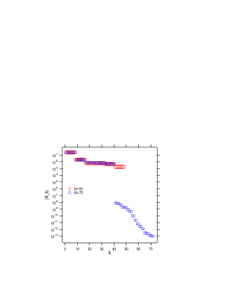
Distribution of poles and zeros of the Pade approximated function $f_{branch2}^{[20|20]}(z)$ to the test function $f_{branch2}(z)$ is shown in Fig.13. The stable poles and zeroes are lined on $[6/5,\infty]$, and the spurious poles appear around $|z|=1$. The magnitude of the residues of the spurious poles is also enormously small compared with those of the stable poles remained as increase of the order of the Pade approximation.

Figure 13: (Color online) (a)Distribution of poles ($\bigcirc$) and zeros ($\times$) of the $[20|20]$ Pade approximated function $f_{branch2}^{[20|20]}(z)$. The unit circle is drawn to guide the eye. (b)Absolute values of the residues $|A_{k}|$ of the $[10|10]$ and $[20|20]$ Pade approximated functions to the test function $f_{branch2}(z)$ without noise. The residues are arranged in descending order.

Figure 14: (Color online) (a)Absolute values of the residues $|A_{k}|$ of the $[50|50]$ Pade approximated functions to the noise added test function $f_{Jac+noise}(z)$ with the strength $\epsilon=0,0.01,0.1$. (b)Absolute values of the residues $|A_{k}|$ of the Pade approximated functions $f^{[50|50]}_{Jac}(z)$, $f^{[32|32]}_{Jac}(z)$, $f^{[64|64]}_{Jac}(z)$ to the test function $f_{Jac}(z)$ without the noise. The residues are arranged in descending order.

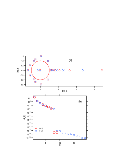
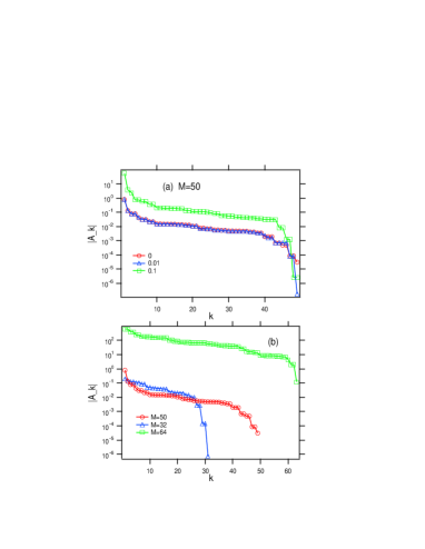
Figure 14 is also the result of the residues analysis for the Pade approximated function to the test function $f_{Jac}(z)$ with a natural boundary on the unit circle $|z|=1$. In the $[50|50]$ Pade approximated function, the magnitude of the residues $|A_{k}|$ is shown in changing the noise strengths $\epsilon=0,0.01,0.1$ corresponding to poles-zeros distribution in Fig.11.

In the small noise case ($\epsilon=0.01$), the results of the residue analysis for $f_{Jac+noise2}(z)$ is almost same as the noise-free case ($\epsilon=0$), and in the case with relatively strong noise ($\epsilon=0.1$), the noise shift the magnitude of the residues larger value. In addition, the result of the residue analysis of the noise-free cases for some different order of the Pade approximation is shown in Fig.14(b). We should have in mind that the order is important when we apply Pade approximation to the lacunary power series because we should not take the order of the approximation in the gap of the series.

VI Froissart doublets

The problem of constructing the $Z-$transform $Z(z)$ of a finite time-series is a standard problem in Mathematics bessis96 ; stahl97 ; gilewicz97 ; bessis09 ; antonio09 . For example, it is shown that for a sum of oscillating damped signals, the $Z-$transform associated with the time-series can be characterized by a sum of the poles of the Pade approximated function. The position of each pole is simply linked to the damping factor and the frequency of each of the oscillators. Also, it is important to note that all these poles lie strictly outside the unit circle because it corresponds to the damping bessis96 ; stahl97 ; gilewicz97 ; bessis09 . In addition, we will consider quasianalyticity property of the random power series by the residue analysis of the Pade approximation.

VI.1 Noise attractor

In signal processing, we can use fact that the poles and zeros of the Pade approximated function to the noisy series distribute around the unit circle $|z|=1$ when we remove the noise from the observed data through $Z-$transform and/or Fourier transform of the data. Let a sequence $\{s_{0},s_{1},....,s_{n},...\}$ as a sample signal without noise. Then we define the $Z-$transform of the sequence as,

$$Z(z)=\sum_{n=0}^{N}s_{n}z^{n}.$$ (40)

The function $Z(z)$ is analytic interior of $|z|<1$ if the number of signal $N$ is finite def . Note that Discrete Fourier transform is a special case of the $Z-$transform.

Next, in the concrete, let us consider a signal sequence in $t\in[0,T]$ consisting of the superimposed damping oscillators as,

$$s_{k}=\sum_{\ell}A_{\ell}e^{i\omega_{\ell}\frac{k}{N}T},k=0,1,...,N-1,$$ (41)

where $A_{\ell}$ is the amplitude of the $\ell-$th oscillator, and $\omega_{\ell}=2\pi f_{\ell}+i\alpha_{\ell}$. Here, $f_{\ell}$ and $\alpha_{\ell}$ are the frequency and the damping factor of the $\ell-$th oscillator. Then, the $Z-$transform is

$$Z(z) = \sum_{n=0}^{\infty}s_{n}z^{n}$$ (42)

$$= \sum_{n=0}^{\infty}\sum_{\ell}A_{\ell}e^{i\omega_{\ell}\frac{n}{N}T}z^{n}$$ (43)

$$= \sum_{\ell}\frac{A_{\ell}}{1-zz_{\ell}},$$ (44)

where we take a limit $n\to\infty$ keeping $T/N$, and $z_{\ell}\equiv e^{i\omega_{\ell}\frac{T}{N}}$. Accordingly, the singularity of $Z(z)$ appears as the poles at $z=z_{\ell}^{-1}\equiv e^{-i\omega_{\ell}\frac{T}{N}}$ outside the unit circle $|z|>1$ and the residue is $Res(z_{\ell}^{-1})=z_{\ell}^{-1}A_{\ell}$.

On the other hand, let us consider a noise-added sequence $\{S_{0},S_{1},....,S_{n},...\}$. Then, the Froissart pointed out that there are two-types of the poles; stable poles and unstable poles when we apply the diagonal Pade approximation to the unknown data set. In general, the $Z-$transform $Z(z)=\sum_{n=0}^{N}S_{n}z^{n}$ of the noisy sequence has a natural boundary on the unit circle $|z|=1$ with probability 1. In fact, the poles and zeros (Froissart doublets) of the Pade approximated function often distribute around the unit circle when the numerical error and/or noise are mixed into the Taylor series of the analytic functions, as seen in the last section. That is to say, we sometimes call the unit circle $|z|=1$ noise attractor in a sense that the poles and zeros are attracted to the circle as the Froissart doublets. Accordingly, it is found that Pade approximated function for the function $Z(z)$ has stable poles associated with the damping modes and unstable spurious poles associated with the noisy fluctuation. After elimination of the spurious poles around the noise attractor from the noisy-sequence we can reconstruct the noise-free sequence consisting of the stable poles located in the domain $|z|>1$. Another remarkable feature of the non-modal poles is that the absolute value of the Cauchy residues associated with them are usually much smaller than those associated with true poles.

VI.2 Random power series and quasianalytic function

Weierstrass defined the analytic function by direct analytic continuation of function. Then, apparently the analytic continuation is impossible beyond the natural boundary even if we can uniquely define the function and it is analytic outside the analytic domain. Borel and Gammel extended the narrow condition for the analyticity and gave a definition of quasianalytic functions Luzin98a ; Luzin98b . Gammel conjectured the following for the random power series gammel73 ; bessis96 .

Gammel conjecture(1973): The random power series belongs to the Borel class of quasianalytic functions as the following form,

$$f_{Gammel}(z)=\sum_{k=0}^{\infty}\frac{B_{k}}{1-w_{k}z},$$ (45)

where $w_{k}=e^{i2\pi X_{k}}$ and $\{X_{k}\}$ are real numbers in the interval in $X_{k}\in[0,1]$, and $B_{k}$ decrease rapidly with $k$. Then natural boundary in the Weierstrass’s sense can be crossed.

The function Eq.(45) is a simple example that poles are densely-distributed on the unit circle. Then the convergence property of the sequence $|B_{k}|$ is important for the analyticity of the function. Carleman proved that $f_{Gammel}(z)$ is quasi-analytic if $B_{k}$ satisfies the following condition

$$|B_{k}|<Ce^{-k^{1+c}},c>0.$$ (46)

This is Carleman-class of quasianalytic functions. See Gammel’s paper gammel73 for the details. Moreover, Gammel and Nuttall proved that the quasianalytic functions can be exactly approximated by the Pade approximation gammel73 .

Gammel-Nuttal Theorem(1973): If $B_{k}$ in Eq.(45) satisfies the condition (46), and $|\omega_{k}|=1$, then, the sequence of $[N+J|N]$ Pade approximation to the $f_{Gammel}(z)$ converges in measure to the function $f_{Gammel}(z)$ as $N\to\infty$ in any closed, bounded region of the complex plane, where $J$ is a natural number that equals to $N$ or less.

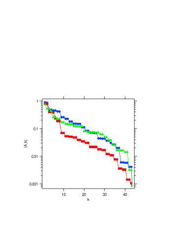
Is the Gammel conjecture true? We try to examine the validity of the Gammel conjecture by applying residue analysis of the Pade approximated function to the random power seres $f_{noise2}(z)$. Figure 15 shows the absolute values of the residues $|A_{k}|$ of the Pade approximated functions $f^{[45|45]}_{noise}(z)$ to three different samples in descending order. $|A_{k}|$ roughly exponentially decreases with respect to $k$ as,

$$|A_{k}|\sim exp(-\beta k),$$ (47)

where $\beta$ is the decay exponent. It shows exponential decay (or faster), and, at the first face, supports the Gammal conjecture.

Figure 15: (Color online) Absolute values of the residues $|A_{k}|$ of the Pade approximated functions $f^{[45|45]}_{noise2}(z)$ to three samples of the truncated random power series of order $N=90$, and $\epsilon=1$. The $|A_{k}|$ are arranged in descending order.

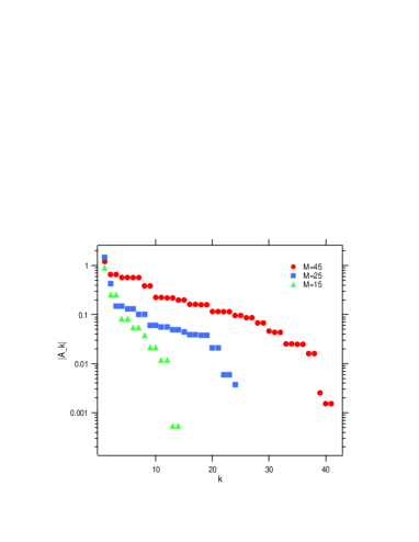
However, it is not nearly so simple. We should check the stability of the exponential-like decay of the magnitude of the residues by changing the order of the Pade approximation. Figure 16 shows the result for the three different orders $M=15$, $M=45$, $M=55$. It express an indication that the decay exponent $\beta$ does not converge a positive certain value. It seems that the exponent behaves $\beta\to 0$ as a limit $M\to\infty$. On the other hand, if we directly apply the Pade approximation to the quasianalytic function $f_{Gammel}(z)$ with $B_{k}={\rm e}^{-k}$, the exponent $\beta$ is stable for changing the order of the Pade approximation. (See appendix E.) These facts suggest that th random power series is not belong to Carleman-class of quasianalytic function although it has a natural boundary on the unit circle, and it has the form (45). As a result, we can say that no optimism is warranted on the Gammel conjecture.

How does the residue analyses of the Pade approximation to analyticity and/or quasianalyticity of unknown function work? It is an interesting and future problem.

Figure 16: (Color online) Absolute values of the residues $|A_{k}|$ of the Pade approximated functions $f^{[45|45]}_{noise2}(z)$, $f^{[25|25]}_{noise2}(z)$, $f^{[15|15]}_{noise2}(z)$ to a sample truncated random series, and $\epsilon=1$. The $|A_{k}|$ are arranged in descending order.

VII Summary and Discussion

In the present paper we numerically examined the effectiveness of the Pade approximation to some test functions with branch point, essential singularity, and natural boundary by watching the singularities of the Pade approximated functions. For the functions with a branch cut, the poles and zeros of the Pade approximated function are lined along the true branch cut. The poles and zeros are distributed around the true natural boundary if the original test function has a natural boundary. In addition, we gave explicit the Pade approximated functions to some lacunary power series which are useful to check the numerical result. It was shown that, in particular, the distribution of poles and zeros of the Pade approximated function to lacunary power series and the random power series accumulated around the unit circle when the order of the approximation increases.

We often suffer from the difficulty to distinguish whether or not the poles of the Pade approximation are intrinsically originated from the natural boundary of the original power series, because the numerical errors contained in the expansion coefficients also yields a false natural boundary. Therefore, the expansion coefficients with adequate numerical accuracy are necessary when we apply the Pade approximation to functions with unknown singularities.

Furthermore, the residue calculus of the Pade approximated function is useful when we detect the singularity of the original power series from the asymptotic behavior of the truncated series. It is useful also for estimating the accuracy of the approximation. As a result, the residue calculus suggests that the random power series does not obey Gammel conjecture, that is, it does not belong to Borel-class of quasianalytic functions.

We finally remark that the most serious problem to be improved is the numerical accuracy due to the limitation of the order in the Pade approximation when we use it for detecting unknown singularities of wave functions in quantum physicsyamada13 .

Appendix A General recursion relation

We can construct a power series that has some pole-type singularities in the following form

$$\frac{dz^{2}+ez+f}{az^{2}+bz+c}=\sum_{n=0}^{\infty}a_{n}z^{n},$$ (48)

where $a,b,c,d,e,f$ are real and $c\neq 0$ for simplicity. Then the coefficients $\{a_{n}\}$ can be obtained by rearranging and comparing with the coefficients of the both sides in the same order as follows,

$$dz^{2}+ez+f=(ba_{0}z+ca_{0}+ca_{1}z)$$ (49)

$$+\sum_{n=2}^{\infty}(aa_{n-2}+ba_{n-1}+ca_{n})z^{n}.$$

As a result, the power series with the pole-type singularities can be constructed by the recursion relation

$$a_{k}=-\frac{b}{c}a_{k-1}-\frac{a}{c}a_{k-2},k\geq 2,$$ (50)

with $ca_{0}=f$, $ba_{0}+ca_{1}=e$, $aa_{0}+ba_{1}+ca_{2}=d$.

It becomes Fibonacci sequence when we set $a_{0}=0,a_{1}=1$, $a_{k}=a_{k-1}+a_{k-2}$.

Appendix B Random polynomial

The following theorems concerning the random power series are well-known.

Erdos-Turan Type theorem(1950): Let us define a polynomial

$$f(z)=\sum_{n=0}^{N}a_{n}z^{n},$$ (51)

where coefficients $a_{n}$ are randomly distributed and $a_{0}a_{N}\neq 0$, for simplicity. Then the zeros of the random polynomial cluster uniformly around the unit circle $|z|=1$ if ”size of the truncated series” $L_{N}(f)$ is small compared to the order $N$ of the polynomial, where

$$L_{N}(f)=\log\left(\frac{\sum_{n=0}^{N}|a_{n}|}{\sqrt{|a_{0}a_{N}|}}\right).$$ (52)

Note that this theorem also hold for the polynomials with deterministic coefficients $a_{n}$ such as Newman type polynomial having coefficients in the sets $\{0,1\}$ or $\{0,\pm 1\}$.

Peres-Virag’s theorem(2005): Let us $\{a_{n}\}$ are i.i.d. Gaussian-type random variables, then the distribution $K(z)$ of the complex zeros $\{z_{k}\}$ of the power series

$$f(z)=\sum_{n=0}^{\infty}a_{n}z^{n},$$ (53)

is

$$K(z_{k})=\frac{1}{\pi}\frac{1}{(1-|z_{k}|^{2})^{2}}.$$ (54)

Appendix C Some Gap Theorems of Lacunary Power Series

Weierstrass considered the analyticity of the power series,

$$f(z)=\sum_{\nu=0}^{\infty}a_{\nu}z^{b^{\nu}},b\in N,b\neq 1,$$ (55)

where $a_{\nu}$ is a positive number. In the main text, we set $a_{\nu}=1$, $b=2$ for $f_{Wei}(z)$. Then, it is proved that the function (55) has a natural boundary on the unit circle $|z|=1$ if the convergence radius of the function is unity based on the following theorems for the lacunary power series.

Hadamard-Barck’s gap theorem(1892): Let us be

$$f(z)=\sum_{\nu=0}^{\infty}a_{\nu}z^{\lambda_{\nu}},$$ (56)

where $a_{\nu}$ is a positive number, and $\{\lambda_{\nu}\}$ denote a strictly increasing sequence of the natural numbers, satisfying a inequality $q\lambda_{\nu}\leq\lambda_{\nu+1}$ for $q>1$. Then the function $f(z)$ has a natural boundary on the unit circle $|z|=1$.

Fabry’s gap theorem(1899): Power series

$$f(z)=\sum_{\nu=0}^{\infty}a_{\nu}z^{\lambda_{\nu}},$$ (57)

with radius of convergence $R=1$ has a natural boundary on the unit circle $|z|=1$, provided it is Fabry series, i.e.

$$\lim_{\nu\to\infty}\frac{\lambda_{\nu}}{\nu}=\infty.$$ (58)

Appendix D Numerators of diagonal Pade approximations to $f_{Jac}(z)$ and $f_{Fib}(z)$

The diagonal Pade approximation to the truncated lacunary power functions $f_{Jac}(z)$ and $f_{Fib}(z)$ can be exactly executed as given in the main text. The numerators $A_{Jac}^{N}(z)$ and $A_{Fib}^{F_{N}}(z)$ of the Pade approximated functions can be given as follows,

$$A^{N}_{Jac}(z) = z+2z^{2}$$

$$+ 2\sum_{n=2}^{N-1}z^{H_{n}}(z+z^{2}+\sum_{k=1}^{n-2}z^{H_{k+2}}),$$

where $H_{n}=2^{n-1}$.

Numerator of the diagonal Pade approximated function to $f_{Fib}(z)$ is

$$A^{F_{N}}_{Fib}(z) = S_{N-4}(z)$$

$$+ [S_{N-8}(z)+z](f_{N-4}(z)-f_{N-2}(z))$$

$$+ [2f_{N-3}(z)+2f_{N-2}(z)+f_{N-3}(z)f_{N-6}(z)],$$

where $S_{L}(z)=\sum_{k=0}^{L}f_{k}(z)$, $f_{k}(z)=z^{F_{k}}$. $F_{N}$ means $N$th Fibonacci number, and we set $F_{-1}=F_{-2}=....=0$.

We have inductively obtained above results by means of MATHEMATICA.

Appendix E Residue analysis for Carleman class of quasianalytic functions

In this appendix, we give a direct result of residue analysis for ”Carleman-class” of the quasianalytic functions, for comparison with the other residue analysis in the main text. We apply the Pade approximation to the qusiperiodic function $f_{Carleman}(z)$ of the Carleman-class, which is artificially constructed by a set of the poles $\{z_{k}\}$ as follows;

$$f_{Carleman}(z) = \sum_{k=1}^{K}(\frac{1}{1-z_{k}z}+\frac{1}{1-z_{k}^{*}z})e^{-k}$$ (61)

$$= 2\sum_{n=0}^{\infty}\sum_{k=1}^{K}e^{-k}\cos(2\pi X_{k}n)z^{n},$$ (62)

where we set the poles at $z_{k}={\rm exp}(\pm 2\pi iX_{k})$ ($k=1,2,...,K$) on the unit circle. $\{X_{k}\}$ are i.i.d random variables in the interval $X_{k}\in[0.1]$ and we take $K=100$. Figure 17 shows the absolute values of the residues $|A_{k}|$ of the Pade approximated functions of order $M=15$, $M=25$, $M=45$ to $f_{Carleman}(z)$. They are arranged in descending order.

Figure 17: (Color online) Absolute values of the residues $|A_{k}|$ of the Pade approximated functions to a truncated Carleman function $f_{Carleman}(z)$ of order $M=15,25,45$, which is artificially constructed by Eq.(62). They are arranged in descending order in each case.

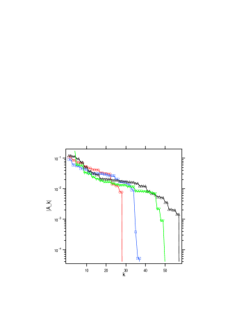
As a result, it seems that $|A_{k}|$ exponentially decreases with a stable exponent, regardless of the order of the Pade approximation. This supports that certainly, the Pade approximation is applicable to the quasianalytic functions in the Gammel conjecture as given in Gammel-Nuttal’s theorem. The Pade approximation for the quasianalytic function converges to the function even outside the unit circle. It should be also noted that in all cases the tails of $|A_{k}|$ are rapidly decay because the ”truncated” series are essentially analytic functions.

Appendix F Some Results for Natural Boundary in Noisy Series

In this appendix some theorems for the random power series are given. See, for example, Ref.remmert10 for the proofs.

Steinhaus’s theorem(1929): Suppose that the power series,

$$f(z)=\sum_{n=0}^{\infty}a_{n}z^{n},$$ (63)

has radius of convergence $R=1$. Let us $X_{0},X_{1},...,X_{n}$ be a sequence of i.i.d. random variables in the interval $X_{i}\in[0,1]$. Then, with probability one, the random power series

$$f_{Steinhaus}(z) = \sum_{n=0}^{\infty}a_{n}w_{n}z^{n},$$ (64)

has a natural boundary on $|z|=1$, where $w_{k}=e^{i2\pi X_{k}}$.

Paley-Zygmund’s theorem(1932): Suppose that the power series (63) has the radius of convergence 1. Let us $r_{0},r_{1},...,r_{n},...$ be a sequence of binary stochastic variables taking $-1$ or $1$ with equal probability. Then, with probability one, the random power series

$$f_{P-Z}(z) = \sum_{n=0}^{\infty}r_{n}z^{n},$$ (65)

has a natural boundary on the unit circle $|z|=1$.

The similar theorems can hold for random power series $\sum_{n=0}^{\infty}r_{n}z^{n}$ with a sequence of stochastic variables obeying i.i.d. in the interval $r_{i}\in[-1,1]$ or $r_{i}\in[0,1]$ kahane85 . The more generalized version has been given in the following form breuer11 .

Breuer-Simon’s theorem(2011): Suppose that the power series (63) has the convergence radius 1. Then for a.e. $\omega$, $f(z)=\sum_{n=0}^{\infty}a_{n}(\omega)z^{n}$ has a strong natural boundary on $|z|=1$ if the $a_{n}(\omega)$ be a stationary, ergodic, bounded, nondeterministic process.

References

- (1) G.A. Baker and J.L. Gammel, The Padé Approximation in Theoretical Physics, (Academic Press: New York, 1970).
- (2) George A. Baker Jr, Essentials of Padé Approximants (Academic Press, 1975).
- (3) George A. Jr Baker and Peter Graves-Morris, Padé Approximants 2nd Edition, (Cambridge University Press, 1996).
- (4) F. Sasagawa, Scattering Theory(Syoukabou, 1991 j (in Japanese).
- (5) H. Stanly, Introduction to Phase Transitions and Critical Phenomena (Clarendon Press, Oxford, 1971).
- (6) C.N. Yang and T.D. Lee, Phys. Rev. 87 (1952) 404.
- (7) B. Nickel, J. Phys.A 32 3889(1999): J. Phys. A 33 1693(2000) .
- (8) R. Kubo, M. Toda, N. Hashizume, and N. Saito, Statistical Physics I, II (Springer-Verlag, Berlin, 1983, 1985).
- (9) B. M. McCoy, arXiv:cond-mat/0103556v1
- (10) D. Bessis, J. Comput. Appl. Math. 66 85-88(1996).
- (11) H. Stahl, J. Comput. Appl. Math. 86 287-296(1997).
- (12) J. Gilewicz and M. Pindor, J. Comput. Appl. Math. 87(1997).
- (13) D. Bessis and L. Perotti, J. Phys. A 42, 365202(2009) .
- (14) L.A. Barbosa Coelho and L.A. Baccala, Pade approximations as a Modal Identification Technique, in Proceedings of the IMAC-XXVII held February 9-12, 2009 Orlando, Florida USA.
- (15) A. Berretti and L. Chierchia, Nonlinearity 3, 39(1990).
- (16) C. Falcolini and R. Llave, J. Stat. Phys. 67, 645(1992).
- (17) R. Llave and S. Tompaidis, Physica D 71, 55(1994).
- (18) A. Berretti and S. Marmi, Chaos, Solitons and Fractals, 5, 257(1995). @
- (19) A. Berretti and C. Falcolini, and G. Gentile, Phs. Rev. E 64, 015202-1(2001). @
- (20) T.W. Korner, Exercises for Fourier Analysis (Cambridge University Press 1993).
- (21) R. Remmert, Classical Topics in Complex Function Theory, (Springer New York; 1st Edition 2010).
- (22) J. Breuer and B. Simon, Advances in Mathematics 226, 4902-4920(2011). arXiv:1002.0823v2 [math.CV].
- (23) O. Knill and J. Lesieutre, ”Analytic continuation of Dirichlet series with almost periodic coefficients”, Complex Analysis and Operator Theory 6, 237-255(2010). arXiv:0811.1362.
- (24) O. Costin and M. Huang, Behavior of lacunary series at the natural boundary, Advances in Mathematics 222, 1370-1404(2009).
- (25) W. H. Press, S. A. Teukolsky, W.T. Vetterling and B.P. Flannery, Numerical Recipes in C (Cambridge University Press, 1988); W. H. Press, S. A. Teukolsky, Computers in Physics, 6, 82(1992).
- (26) P. Gonnet, R. Pachon, and L. N. Trefethen, Electronic Transactions on Numerical Analysis 38, 146-167(2011).
- (27) P. Gonnet, S. Guttel, and L. N. Trefethen, Robust Pade Approximation via SVD, SIAM Review 55, 101-117(2013).
- (28) M. Kac, Bull. Amer. Math. Soc. 49, 314-320(1943).
- (29) P. Erdos and P. Turan, Annals of Mathematics 51, 105-119(1950).
- (30) F. Amoroso and M. Mignotte, Ann. Inst. Fourier 46, 1275-1291(1996).
- (31) A. Odlyzko and B. Poonen, Enseign. Math. 39, 317-348 (1993).
- (32) B.Simon, Orthogonal Polynomials on the Unit Circle, part 1:Classical Theory, (American Mathematical Society 2004).
- (33) B.Simon, Orthogonal Polynomials on the Unit Circle, part 2:Spectral Theory, (American Mathematical Society 2004).
- (34) Y. Peres and B. Virag, Acta Math. 194, 1-35(2005).
- (35) B.Simon, Szego’s Theorem and Its Descendants: Spectral Theory for L2 Perturbations of Orthogonal Polynomials, (Princeton University Press 2010).
- (36) Abe Shenitzer,N. Luzin, ”Function: Part I”, The American Mathematical Monthly, 105, 59-67(1998).
- (37) N. Luzin, ”Function: Part II”, The American Mathematical Monthly, 105, 263-270(Mar., 1998).
- (38) We can also define the transform by negative power . Then the function is analytic in outer domain of , the poles corresponding to damping oscillations appear in the inside the unit circle .
- (39) J.L. Gammel and J. Nuttal, J. Math. Anal. Appl. 43, 694-696(1973).
- (40) H.S.Yamada and K.S. Ikeda, ”Analyticity of Quantum States in One-Dimensional Tight-Binding Model”, preprint (2014).
- (41) J.-P. Kahane, Some Random Series of Functions, 2nd edition, Cambridge Studies in Advanced Mathematics, 5, (Cambridge University Press, Cambridge, 1985).