CANDELS Multi-wavelength Catalogs: Source Detection and Photometry in the GOODS-South Field
Abstract
We present a UV-to-mid infrared multi-wavelength catalog in the CANDELS/GOODS-S field, combining the newly obtained CANDELS HST/WFC3 F105W, F125W, and F160W data with existing public data. The catalog is based on source detection in the WFC3 F160W band. The F160W mosaic includes the data from CANDELS deep and wide observations as well as previous ERS and HUDF09 programs. The mosaic reaches a 5 limiting depth (within an aperture of radius 017) of 27.4, 28.2, and 29.7 AB for CANDELS wide, deep, and HUDF regions, respectively. The catalog contains 34930 sources with the representative 50% completeness reaching 25.9, 26.6, and 28.1 AB in the F160W band for the three regions. In addition to WFC3 bands, the catalog also includes data from UV (U-band from both CTIO/MOSAIC and VLT/VIMOS), optical (HST/ACS F435W, F606W, F775W, F814W, and F850LP), and infrared (HST/WFC3 F098M, VLT/ISAAC Ks, VLT/HAWK-I Ks, and Spitzer/IRAC 3.6, 4.5, 5.8, 8.0 m) observations. The catalog is validated via stellar colors, comparison with other published catalogs, zeropoint offsets determined from the best-fit templates of the spectral energy distribution of spectroscopically observed objects, and the accuracy of photometric redshifts. The catalog is able to detect unreddened star-forming (passive) galaxies with stellar mass of at a 50% completeness level to z3.4 (2.8), 4.6 (3.2), and 7.0 (4.2) in the three regions. As an example of application, the catalog is used to select both star-forming and passive galaxies at z2–4 via the Balmer break. It is also used to study the color–magnitude diagram of galaxies at 0z4.
1. Introduction
Over the past decade, the Hubble Space Telescope (HST) and modern giant telescopes have opened a new era in observational cosmology. Galaxies are now routinely found in the very early universe, and their evolution can be followed from its early stages to the present. Particularly, deep multi-wavelength imaging surveys have been established as a powerful and efficient tool to push observations up to high redshift and down to faint populations of galaxies. These modern surveys have revealed a complex interplay between galaxy mergers, star formation, and black holes over cosmic time and have led to new insights into the physical processes that drive galaxy formation and evolution.
Of the entire cosmic time, two epochs are particularly of great interest: z2 (Cosmic High Noon) and z8 (Cosmic Dawn). In the former, the cosmic star formation history reached its peak (e.g., Hopkins, 2004; Hopkins & Beacom, 2006; Bouwens et al., 2009), and galaxies quickly assembled their stars (e.g., Daddi et al., 2007; Reddy et al., 2008; Reddy & Steidel, 2009) as well as began to differentiate into morphological sequence (e.g., Cassata et al., 2008; Kriek et al., 2009; Whitaker et al., 2011; Wang et al., 2012). In the latter, detection and physical properties of galaxies place essential constraints on the reionization (e.g., Fontana et al., 2010; Oesch et al., 2010; Grazian et al., 2011; Bouwens et al., 2012; Finkelstein et al., 2012a), the accretion history of galaxies at early times (e.g., Bouwens et al., 2010a; Finkelstein et al., 2010; McLure et al., 2010; Trenti et al., 2011; Yan et al., 2012) as well as the formation of metals and dust in the intergalactic medium (e.g., Bouwens et al., 2010b; Dunlop et al., 2012; Finkelstein et al., 2012b). Because two important spectral features, namely, the Balmer break at z2 and the Lyman break at z8, are redshifted to near-infrared (NIR) bands at the two epochs, a NIR survey with deep sensitivity and high spatial resolution is required for robust investigation of galaxies during these epochs. Incorporating these deep NIR data into a multi-wavelength catalog would significantly improve measurements of galaxy properties at z2.
The Cosmic Assembly Near-infrared Deep Extragalactic Legacy Survey (CANDELS, Grogin et al., 2011; Koekemoer et al., 2011) is designed to document galaxy formation and evolution over the redshift range of z=1.5–8. The core of CANDELS is to use the revolutionary near-infrared HST/WFC3 camera, installed on Hubble in May 2009, to obtain deep imaging of faint and faraway objects. CANDELS also uses HST/ACS to carry out parallel observations, aiming to providing unprecedented panchromatic coverage of galaxies from optical wavelengths to the near-IR. Covering approximately 800 , CANDELS will image over 250,000 distant galaxies within five popular sky regions which possess rich existing data from multiple telescopes and instruments: GOODS-S, GOODS-N, UDS, EGS, and COSMOS. The strategy of five widely separated fields mitigates cosmic variance and yields statistically robust and complete samples of galaxies down to a stellar mass of to z2, and around the knee of the ultraviolet luminosity function of galaxies to z8. It will also find and measure Type Ia supernovae at z1.5 to test their accuracy as standard candles for cosmology.
The GOODS-S field, centered at (J2000) = 03h32m30s and (J2000) = -27d48m20s and located within the Chandra Deep Field South (CDF-S, Giacconi et al., 2002), is a sky region of about 170 arcmin2 which has been targeted for some of the deepest observations ever taken by NASA’s Great Observatories: HST, Spitzer, and Chandra as well as by other world-class telescopes. The field has been imaged in the optical wavelength with HST/ACS in F435W, F606W, F775W, and F850LP bands as part of the HST Treasury Program: the Great Observatories Origins Deep Survey (GOODS, Giavalisco et al., 2004); in the mid-IR (3.6–24 m) wavelength with Spitzer as part of the GOODS Spitzer Legacy Program (PI: M. Dickinson); and in the X-ray with the deepest Chandra sky survey ever taken, with a total integration time of 4 Ms (Xue et al., 2011). The field also has very deep far-IR to submillimeter data from Herschel Space Observatory from the PEP survey (Lutz et al., 2011) and the HerMes survey (Oliver et al., 2012), deep submillimeter (1.1 mm) observation with AzTEC/ASTE (Scott et al., 2010), and radio imaging from the VLA (Kellermann et al., 2008), ATCA (Norris et al., 2006; Zinn et al., 2012), and VLBA (Middelberg et al., 2011). Furthermore, the field has been the subject of numerous spectroscopic surveys (e.g., Le Fèvre et al., 2004; Szokoly et al., 2004; Mignoli et al., 2005; Cimatti et al., 2008; Vanzella et al., 2008; Popesso et al., 2009; Balestra et al., 2010; Silverman et al., 2010). These rich and deep existing data, covering the full wavelength range, make GOODS-S one of the best fields to study galaxy formation and evolution.
This paper presents a multi-wavelength catalog of GOODS-S based on CANDELS WFC3 F160W detection, combining both CANDELS data and available public imaging data from UV to mid-IR wavelength. The catalog includes U-band images obtained with the CTIO Blanco telescope and with the Visible Multi-Object Spectrograph (VIMOS) on the Very Large Telescope (VLT), HST/ACS images in F435W, F606W, F775W, F814W, and F850LP bands, HST/WFC3 images in F098M, F105W, F125W, and F160W bands, Ks-band image with the Infrared Spectrometer and Array Camera (ISAAC) and the High Acuity Wide field K-band Imager (HAWK-I) on the VLT, as well as Spitzer images at 3.5, 4.5, 5.8, and 8.0 m.
The paper is organized as follows: Sec. 2 briefly summarizes the datasets included in our catalog. Sec. 3 discusses source detection in the CANDELS F160W image and photometry measurement on HST images. Sec. 4 discusses photometry measurements on low resolution images. Sec. 5 evaluates the quality of our photometry catalog. Sec. 6 presents a few simple applications of our catalog to study galaxy formation and evolution. The summary is given in Sec. 7.
All magnitudes in the paper are on the AB scale (Oke, 1974) unless otherwise noted. We adopt a flat cosmology with , and use the Hubble constant in terms of .
The CANDELS GOODS-S multi-wavelength catalog and its associated files — all SExtractor photometry of the HST bands as well as the system throughput of all included filters — are made publicly available on the CANDELS Website111http://candels.ucolick.org, in the Mikulski Archive for Space Telescopes (MAST)222http://archive.stsci.edu, via the on-line version of the article, and the Centre de Donnees astronomiques de Strasbourg (CDS). They are also available in the Rainbow Database333US: https://arcoiris.ucolick.org/Rainbow_navigator_public, and Europe: https://rainbowx.fis.ucm.es/Rainbow_ navigator_public. (Pérez-González et al., 2008; Barro et al., 2011), which features a query menu that allows users to search for individual galaxies, create subsets of the complete sample based on different criteria, and inspect cutouts of the galaxies in any of the available bands. It also includes a cross-matching tool to compare against user uploaded catalogs.
2. Data
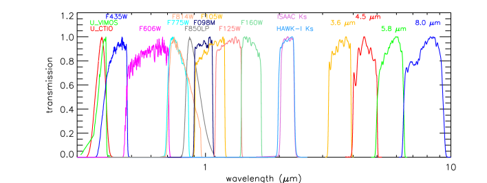
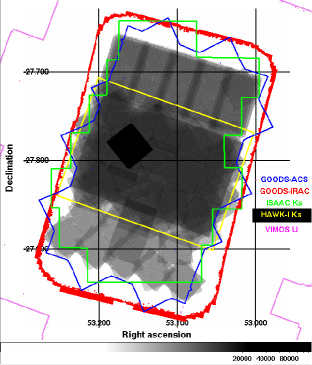
Table 1 summarizes the multi-wavelength datasets included in our catalog. The table lists the effective wavelength, the full width at half-maximum (FWHM) of the filter, the FWHM of the point spread function (PSF), and the limiting magnitude of each band in our catalog. For each band, we calculate the 5 limiting magnitude with an aperture whose radius is equal to the FWHM of the band. No aperture correction is applied to the limiting magnitude. Transmission curves of all filters used in our catalog are plotted in Figure 1. The sky coverage of observations used in our catalog is shown in Figure 2.
| Instrument | Filter | Effective | Filter | PSF | 5 Limiting |
|---|---|---|---|---|---|
| Wavelength111Effective wavelength is calculated as: (Tokunaga & Vacca, 2005) | FWHM | FWHM | Depth | ||
| (Å) | (Å) | (arcsec) | (AB)222Aperture magnitude at 5 within FWHM of the PSF. Point source magnitude will be brighter than this by the aperture correction assuming the profile of the PSF. Aperture corrections for extended sources will depend on their surface-brightness profiles. | ||
| Blanco/MOSAIC II | U_CTIO | 3734 | 387 | 1.37 | 26.63 |
| VLT/VIMOS | U_VIMOS | 3722 | 297 | 0.80 | 27.97 |
| HST/ACS | F435W | 4317 | 920 | 0.08 | 28.95 / 30.55333The limiting depths of ACS bands are measured within apertures with a fixed radius of 009. Each band has two measurements: one for GOODS-S V2.0 and the other for HUDF. |
| F606W | 5918 | 2324 | 0.08 | 29.35 / 31.05c | |
| F775W | 7693 | 1511 | 0.08 | 28.55 / 30.85c | |
| F814W | 8047 | 1826 | 0.09 | 28.84 | |
| F850LP | 9055 | 1236 | 0.09 | 28.55 / 30.25c | |
| HST/WFC3 | F098M | 9851 | 1696 | 0.13 | 28.77 |
| F105W | 10550 | 2916 | 0.15 | 27.45 / 28.45 / 29.45444The limiting depths of WFC3 bands are measured within apertures with a fixed radius of 017. Each band has three measurements: for CANDELS-wide, CANDELS-deep, and HUDF09, respectively. | |
| F125W | 12486 | 3005 | 0.16 | 27.66 / 28.34 / 29.78d | |
| F160W | 15370 | 2874 | 0.17 | 27.36 / 28.16 / 29.74d | |
| VLT/ISAAC | Ks | 21605 | 2746 | 0.48555PSF and depth vary among ISAAC tiles. We show the median and the 15 and 85 percentiles of all available tiles. | 25.09 e |
| VLT/HAWK-I | Ks | 21463 | 3250 | 0.4 | 26.45 |
| Spitzer/IRAC | 3.6m | 35508 | 7432 | 1.66 | 26.52666This is the depth of the SEDS GOODS-S region measured through apertures. For the SEDS non-GOODS region, the 5 depth is 25.4 AB mag measured through photometry of artificial sources. Ashby et al. (2013) give details of the depth of SEDS depths. |
| 4.5m | 44960 | 10097 | 1.72 | 26.25f | |
| 5.8m | 57245 | 13912 | 1.88 | 23.75777This is the average depth of the two GOODS Spitzer epochs. The overlapped region, which is in the CANDELS-deep region, is deeper by about 0.35 mag. | |
| 8.0m | 78840 | 28312 | 1.98 | 23.72g |
2.1. HST/WFC3 Imaging
Several programs have carried out observations with HST/WFC3 IR channels in GOODS-S, including CANDELS, the HST/WFC3 Early Release Science (ERS, Windhorst et al., 2011), and HUDF09 (Bouwens et al., 2010a). To maximize the scientific merit of our multi-wavelength catalog, we combine all published HST/WFC3 imaging within GOODS-S prior to June, 2012 to make a “max-depth” co-added mosaic of HST/WFC3 images. These co-added images provide each source the deepest NIR observation to date to ensure the least uncertainty when these bands are used for measuring photometric redshifts and stellar masses. A potential drawback is the inhomogeneity of the depth across the whole GOODS-S field, which may bring complexity for measuring the completeness of the catalog. However, even within each sub-region of the field, for example the CANDELS wide region, the actual point-by-point exposure times and sensitivities vary considerably. Therefore, the inhomogeneity issue exists anyway.
CANDELS observed GOODS-S with the HST/WFC3 F105W, F125W, and F160W filters using two strategies: deep and wide. The deep region covers the middle one-third of the GOODS-S ACS region with an area of 55 arcmin2 by 3, 4, and 6 orbits with the F105W, F125W, and F160W filters, respectively. The wide region covers the southern one-third of the GOODS-S ACS region and has approximately 1-orbit exposure for all three bands. Grogin et al. (2011) and Koekemoer et al. (2011) give details of CANDELS HST/WFC3 observations, survey design, and data reduction. The GOODS-S region was also observed by CANDELS with the HST/ACS F814W filter in parallel.
The northern one-third of the GOODS-S region was observed by HST/WFC3 ERS (Windhorst et al., 2011) with the F098M, F125W, and F160W filters. ERS covered this region with 2 orbits in each of the three bands.
An area of about 4.6 arcmin2 in GOODS-S, the Hubble Ultra Deep Field (HUDF), is covered by ultra-deep HST/WFC3 imaging from G. Illingworth’s HUDF09 program (GO 11563, Bouwens et al., 2010a). HUDF09 observed the field for 24, 34, and 53 orbits in the F105W, F125W, and F160W bands. The CANDELS deep/wide region and ERS, together with the Hubble Ultra Deep Fields, create a three-tiered “wedding-cake” approach that has proven efficient for extragalactic surveys. We carry out our own data reduction on both ERS and HUDF images and drizzled them to 006/pixel to match our CANDELS pixel scale (see Koekemoer et al., 2011, for details). The distributions of exposure time and limiting magnitude of our max-depth F160W mosaic are shown in Figure 3.

2.2. HST/ACS Imaging
The HST/ACS images used in our catalog are the version v3.0 of the mosaicked images from the GOODS HST/ACS Treasury Program. They consist of data acquired prior to the HST Servicing Mission 4, including mainly data of the original GOODS HST/ACS program in HST Cycle 11 (GO 9425 and 9583; see Giavalisco et al., 2004) and additional data acquired on the GOODS fields during the search for high redshift Type Ia supernovae carried out during Cycles 12 and 13 (Program ID 9727, P.I. Saul Perlmutter, and 9728, 10339, 10340, P.I. Adam Riess; see, e.g., Riess et al., 2007). The GOODS-S field was observed in ACS B, V, i, and z-band with a total exposure time of 7200, 5450, 7028, and 18232 seconds.
2.3. Ground-based Imaging
GOODS-S is covered by a large number of ground-based images. Combined into our catalog is imaging of CTIO U-band, VLT/VIMOS U-band, VLT/ISAAC Ks-band, and VLT/HAWK-I Ks-band.
The CDF-S/GOODS field was observed by the MOSAIC II imager on the CTIO 4m Blanco telescope to obtain deep U-band observations in September, 2001. The observations were taken through CTIO filter c6021, the SDSS u′ filter111A red leak is found in the filter, between 7000 and 11000 Å. The red leak affects the photometry of objects with red colors. Smith et al. (2002) found that the red leak makes objects with red color (u′-i5 mag) brighter in the u′-band than they should be.. This filter was chosen in order to minimize bandpass overlap with the standard B-band and the ACS F435W filter in hope of providing better photometric redshift and Lyman break constraints on z3 galaxies. The final image has a total integration time of about 17.5 hours.
Another U-band survey in GOODS-S was carried out using the VIMOS instrument mounted at the Melipal Unit Telescope of the VLT at ESO’s Cerro Paranal Observatory, Chile. This large program of ESO (168.A-0485, PI C. Cesarsky) was obtained in service mode observations in UT3 between August 2004 and fall 2006, with a total time allocation of 40 hours. Nonino et al. (2009) give details of the U-band imaging.
In the ground-based NIR, imaging observations of the CDF-S were carried out in J, H, Ks bands using the ISAAC instrument mounted at the Antu Unit Telescope of the VLT. Data were obtained as part of the ESO Large Programme 168.A-0485 (PI: C. Cesarsky) as well as ESO Programmes 64.O-0643, 66.A-0572 and 68.A-0544 (PI: E. Giallongo) with a total allocation time of 500 hours from October 1999 to January 2007. The data cover 172.4, 159.6, and 173.1 arcmin2 of the GOODS/CDF-S region in J, H, and Ks, respectively. Because the CANDELS HST/WFC3 F125W and F160W bands surpass the ground-based J- and H-bands in both spatial resolution and sensitivity, we use only the Ks data from the GOODS VLT/ISAAC program. Retzlaff et al. (2010) give details of the ISAAC Ks-band imaging.
The CANDELS/GOODS-S field was also observed in the NIR as part of the ongoing HAWK-I UDS and GOODS-S survey (HUGS; VLT large program ID 186.A-0898, PI: A. Fontana; Fontana et al. in prep.) using the High Acuity Wide field K-band Imager (HAWK-I) on VLT. Included in this paper are the two deep HAWK-I pointings in the CANDELS deep region. Each pointing was imaged in the Ks-band for 31 hours. Fontana et al. (in preparation) will give more details of the HUGS survey and data.
2.4. Spitzer/IRAC Imaging
GOODS-S was observed by Spitzer/IRAC (Fazio et al., 2004) with four channels (3.6, 4.5, 5.8, and 8.0 m) in two epochs with a separation of six months (February 2004 and August 2004) by the GOODS Spitzer Legacy project (PI: M. Dickinson). Each epoch contained two pointings, each with total extent approximately 10 arcmin on a side. IRAC observed simultaneously in all four channels, with channels 1 and 3 (3.6 and 5.8 microns) covering one pointing on the sky and channels 2 and 4 (4.5 and 8.0 microns) covering another pointing. After two epochs, GOODS-S has complete coverage in all four IRAC channels with an overlap strip in the middle receiving twice the exposure time of the rest of the field. The exposure time per channel per sky pointing was approximately 25 hours per epoch and doubled in the overlap strip. We include the GOODS 5.8 and 8.0 m imaging in our catalog.
The Spitzer/IRAC 3.6 and 4.5 m images used here were drawn from the Spitzer Extended Deep Survey (SEDS; PI G. Fazio; Ashby et al., 2013). The SEDS ECDFS observations were acquired during three separate visits made during the warm Spitzer mission. Each SEDS visit covered a region surrounding the existing IRAC exposures from the GOODS program, and the SEDS mosaics incorporate the pre-existing cryogenic observations. The SEDS mosaics were pixellated to 06 and were constructed with a tangent-plane projection designed to match that of the CANDELS HST/WFC3 mosaics. Total 3 depths in the SEDS-only portions of the field are 26 AB mag measured through photometry of artificial sources. Catalogs and source counts in the 3.6 and 4.5 m mosaics are fully described by Ashby et al. (2013).
3. Photometry of HST Images
3.1. Source Detection in Max-depth F160W Image
The scientific goals of CANDELS extend from studying the morphology of galaxies at the cosmic high-noon (z2) to searching for faint galaxies at the cosmic dawn (z7). Therefore, our source detection strategy must be efficient in detecting both bright/large and faint/small sources. It is, however, almost impossible to design a single set of SExtractor parameters to achieve this goal. A mild detection and deblending threshold avoids breaking large/bright sources into small pieces but misses a large fraction of faint sources. On the other hand, an aggressive detection threshold able to detect very faint sources over-deblends bright/large galaxies. To ensure that our catalog provides reliable detection for both the bright/large and faint/small sources, we adopt a two-mode detection strategy, which has been shown to be successful and efficient in other deep sky surveys, e.g., GEMS (Rix et al., 2004) and STAGES (Gray et al., 2009).
We run our modified SExtractor (see Galametz et al., 2013) on our co-added max-depth version of HST/WFC3 F160W image to detect sources in two modes: “cold” and “hot”. In the cold mode, the SExtractor configuration is designed to detect bright/large sources without over-deblending them. In the hot mode, the SExtractor configuration is pushed to detect faint sources toward the limiting depth of the image. In this mode, bright/large sources may be dissolved, and some of their sub-structures are treated as independent sources. We then follow the strategy of GALAPAGOS (Barden et al., 2012) to merge the two modes: all cold sources are kept into the final detection catalog, but hot sources within the Kron radius of any cold sources are treated as sub-structures of the cold sources and excluded from the final catalog. Only the hot sources that are not within the Kron radius of any cold sources are included in the final catalog. We refer readers to GALAPAGOS (Barden et al., 2012) and Galametz et al. (2013) for details of this two-mode strategy and its application on CANDELS images. In total, we detect 34930 sources from our max-depth F160W mosaic. Among them, 26835 sources are detected by the cold mode and 8095 sources by the hot mode. The key SExtractor parameters used in our source detection are listed in Table 2.
The inhomogeneous depth across our detection image brings a new issue on the detection and deblending threshold. Ideally, in order to construct a catalog whose completeness is similar over regions with various depths, one would use a distinct configuration for each region or use a fixed surface brightness threshold instead of signal-to-noise ratio (S/N) to detect sources. In our catalog, however, we use the same S/N threshold for detecting sources in all regions. The choice is based on two facts. First, the purpose of our max-depth catalog is to push our detection ability in each region to its limit. Therefore, it is the limit on the faint end instead of a homogeneous completeness that we are interested in. Second, even within one region, the depth varies from point to point due to the observation pattern. For example, in the “wide” region, the exposure time of points observed by more than one tile could be 3–4 times higher than that of points observed only once. Because the inhomogeneity exists not only between different regions but also within each region, it would be impossible to design a distinct detection configuration for each region. For readers who are interested in completeness, the catalog provides the exposure time (or depth) of each source, which can be used to construct a sample that is complete to the same depth over all regions.
| Cold Mode | Hot Mode | |
| DETECT_MINAREA | 5.0 | 10.0 |
| DETECT_THRESH | 0.75 | 0.7 |
| ANALYSIS_THRESH | 5.0 | 0.8 |
| FILTER_NAME | tophat_9.0_9x9.conv | gauss_4.0_7x7.conv |
| DEBLEND_NTHRESH | 16 | 64 |
| DEBLEND_MINCONT | 0.0001 | 0.001 |
| BACK_SIZE | 256 | 128 |
| BACK_FILTERSIZE | 9 | 5 |
| BACKPHOTO_THICK | 100 | 48 |
| MEMORY_OBJSTACK | 4000 | 4000 |
| MEMORY_PIXSTACK | 400000 | 400000 |
| MEMORY_BUFSIZE | 5000 | 5000 |
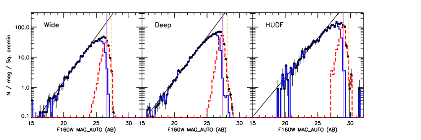
The differential number densities of sources detected in the three (wide, deep + ERS, and HUDF) regions are shown in Figure 4. We also separate the contributions of sources detected in the cold and hot modes. In all regions, the distribution peak of the hot-detected sources is almost 1–1.5 magnitude fainter than that of the cold-detected ones. The hot mode significantly improves our detection ability toward the limiting depth of our images. To make a fair comparison between the total magnitude (MAG_AUTO) of detected sources and the limiting depth, we correct the 5 limiting depths of the F160W band in Table 1, which is measured within an aperture, to include the light outside the aperture by assuming the light profile of the F160W PSF. The peak of the hot detected sources matches the corrected depth (purple line) very well in all regions. Compared to the cold mode, the hot mode boosts the source number density at the limiting depth by a factor of 20.

The differential number density provides a rough way to estimate the completeness of our catalog in different regions. We fit a power law to the differential number density of each region. The catalog probably becomes incomplete when the actual differential number density significantly deviates from the best-fit power law at the faint end. We only fit the power law in the magnitude range in which the catalog is believed to be complete as well as has good number statistics: 20–24 mag, 20–24 mag, and 21–26 mag for the wide, deep, and HUDF regions, respectively. The actual differential number density becomes lower than the best-fit power law by a factor of two at 25.9, 26.6, and 28.1 mag for the three regions. Therefore, our catalog is 50% complete at these magnitudes for the three regions.
This completeness is only a rough estimate. It depends on the assumption that our catalog is complete in the fitting range. What is more, it assumes that the completeness only depends on the flux of sources. It also assumes the counts are a power law over the magnitude range that was fit, and that this power law extends to fainter magnitudes. In fact, the completeness depends on the flux, size, and even morphology of sources. The completeness estimated here is just an overall value for objects with mixed types and should be used with caution when dealing with a specific type of object.
In order to accurately estimate the completeness of sources with various fluxes, sizes, and light profiles, we carry out Monte Carlo simulations of detecting fake sources with the same detection strategy used in our catalog for each region. The fake galaxies populate the magnitude range of 20 mag F160W 30 mag and the range of galaxy half-light radii from 0.1 pixel to 30 pixels. The input galaxies are spheroids with a de Vaucouleurs surface brightness profile (Sérsic index ) and disks with an exponential profile (). The simulated galaxies are convolved with the F160W PSF and inserted into our F160W mosaic with additional Poisson noise. We use the SExtractor parameters of both our cold and hot modes to recover the fake sources. The resulting completeness limits in a plane of magnitude and half-light radius are shown in Figure 5.
In this figure, we over-plot the power-law estimated 50% completeness at the median size (the half-light radius measured by SExtractor) of sources in each region. These values are in good agreement with those measured by the simulation for sources with the input size similar to the median of the actual size distribution. The 20 and 80 percentiles of the actual size distributions span a fairly small range of about 0.3 dex, within which the 50% completeness measured through the simulation changes mildly for each region. Therefore, the 50% completeness estimated from the power law can be used as a representative limit for the majority of sources in our catalog. For sources with much larger sizes, however, their completeness is much worse than this representative value. The completeness also depends on the morphology of sources. Sources with higher light concentration () are complete to fainter magnitude than those with lower concentration () at the same radius.
3.2. Photometry of Other HST Images
Photometry of other HST bands, namely, ACS F435W, F606W, F775W, F814W, F850LP and WFC3 F098M, F105W, and F125W, is measured by running SExtractor in dual-image mode with our WFC3 F160W mosaic as the detection image. All these bands are smoothed by using the IRAF/PSFMATCH package111We set the PSFMATCH parameters “filter”=“replace” and “threshold”=0.01 to replace the very high-frequency and low signal-to-noise components of the PSF matching function with a model computed from the low frequency and high signal-to-noise components of the matching function. to match their PSFs to that of the F160W image. The WFC3 PSFs are generated by combining a core from TinyTim and wing from stacked stars (see van der Wel et al., 2012, for details), while the ACS PSFs are generated by stacking stars. SExtractor is run on the PSF-matched image of each band in both cold and hot modes with the same configurations as used for the F160W photometry. Therefore, the source detection, segmentation area, and isophotal area of sources are identical for the F160W and other HST images. The cold and hot photometry of each band is merged based on the F160W cold and hot detection and combination.
Because the isophotal areas of a source in all HST bands are identical, the isophotal fluxes (FLUX_ISO in SExtractor) can be used to measure colors among the HST bands. Under some circumstances, e.g., measuring stellar mass from spectral energy distribution (SED) fitting, the total fluxes of all bands are needed. For these purposes, we provide an inferred total flux for each band in the following way. For the detection band (F160W), we use the photometry from within the Kron elliptical aperture (FLUX_AUTO in SExtractor) as the measure of total flux. We then derive an aperture correction factor, , and apply it to other HST bands to convert their isophotal fluxes and uncertainties into the total fluxes and uncertainties: FLUX_TOTAL = FLUX_ISO and FLUXERR_TOTAL = FLUXERR_ISO. Our aperture correction method provides an accurate estimate of colors and fluxes subject to the prior assumption that the PSF-convolved profile is the same in all bands. While this assumption is not likely to hold for well-resolved sources, most of the sources in the image are small enough that any wavelength dependence of the galaxy profile will have very little impact on the integrated flux ratio. The total flux and its uncertainty (FLUX_TOTAL and FLUXERR_TOTAL) are provided in the catalog.
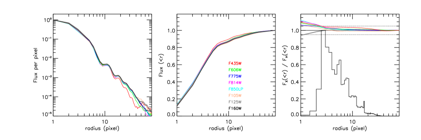
The accuracy of the PSF matching is crucial to our HST photometry. To test it, we extract stars from the CANDELS deep region (to ensure a relatively high S/N) from all PSF-matched HST images and compare their light profiles and curves of growth in Figure 6. The curves of growth of all HST bands, normalized by that of the F160W band, quickly converge to unity after a few pixels. If the radius of the isophotal aperture of a source is larger than two pixels (012), the relative error of isophotal fluxes in all HST bands is less than 5%. Overall, our PSF-matching does not induce a significant systematic offset for the bulk of our sources. Only 2.5% of sources in our sample have isophotal radii less than 2 pixels. For them, the relative photometric systematic offsets or uncertainties induced by PSF-matching could be larger than 5%. For these sources, we enforce a minimum aperture with radius of 2.08 pixels (0125). Fluxes within the minimum aperture (SExtractor parameter FLUX_APER) instead of FLUX_ISO are used for these sources in all HST bands. The aperture fluxes and uncertainties are then scaled up by a new aperture correction factor, of the F160W band, to convert into the total fluxes and uncertainties.
3.3. HST Noise Properties
The uncertainties of our HST photometry are essentially the SExtractor FLUXERR_ISO parameter scaled by an aperture correction factor. Recent works (e.g., Wuyts et al., 2008; Coe et al., 2013) have suggested that this parameter may underestimate the true photometric uncertainties by a significant factor (up to 2–3), primarily due to the pixel-to-pixel correlations that are induced by the step of drizzle (e.g., Casertano et al., 2000) in the image reduction/combination process.
However, in our case we provide SExtractor an RMS map for each filter that has already been corrected for the correlations. Our pipeline that generates the drizzled HST images also produces a weight map whose value is nominally the inverse variance of the expected background noise, predicted using a noise model for the instrument that takes into account the background level, the exposure time, and the expected instrumental noise. In principle, this weight map should correctly describe the actual image noise. However, the noise in the drizzled science images is suppressed by the pixel-to-pixel correlations. We measure the background noise and the factor by which it is suppressed using an IRAF script “acall”, originally developed for GOODS (M. Dickinson, private communication). The script runs on a relatively empty region of the image with relatively uniform exposure time . After masking our objects in the image and removing any low-level background variations by median filtering on large angular scales, the script computes the auto-correlation function of the unmasked pixels. The 2D auto-correlation image typically has a strong peak and falls off sharply on a scale of a few drizzled pixels, since the data reduction (mainly drizzling) does not introduce correlations on scales much larger than 1 or 2 original detector pixels. The script measures the peak value of the auto-correlation image and the total power integrated out to some small radius that can be set interactively. The square root of this ratio (peak over total) is the RMS suppression factor () due to the pixel-to-pixel correlations. The measured inverse variance, corrected for the correlations, is therefore . This is compared to the value predicted from the weight map produced by the drizzle pipeline, and if necessary the weight map is re-scaled accordingly. The final RMS map used for photometry is then computed from the inverse square root of the re-scaled weight map.
We carry out a test, equivalent to the “empty aperture” method of measuring the variance within empty apertures of various sizes placed throughout the images (e.g., Wuyts et al., 2008; Whitaker et al., 2011; Coe et al., 2013), to examine the noise properties of our HST images. First, we mask out all detected sources in the HST images. Then, for each band, we block sum both the drizzled science image and the variance map (square of the RMS map) with various block sizes (, in unit of pixel). Each block can be treated as an “empty box”. We then calculate the ratio of the background RMS of the summed science image and the median of the summed RMS map (square root of the summed variance map). The ratio should be equal to unity if the pixel-to-pixel correlations are corrected.
Figure 7 shows the ratio as a function of in the wide, deep, and HUDF regions of the F160W image. The ratio is close to 1 at 5rb13, demonstrating that our RMS map represents the background noise correctly on the scales relevant for most of our sources in the image, whose typical sizes are 7 pixels. At rb13, the background RMS is larger than the median of the RMS map, mainly due to the unmasked wings of detected objects and undetected sources, which contaminate most blocked pixels when is large. It could also be due to any larger scale fluctuations not removed by the flat fielding and sky subtraction steps of the data processing. This effect is strongest in the HUDF region because it has the highest source number density and detects more extended wings of objects than the other two regions.
The effect of correlation noise becomes more severe at smaller scale. At =1, the background RMS is lower than the median of the RMS map by a factor of 23, implying that the unblocked pixel-to-pixel RMS would significantly underestimate photometric uncertainties due to the correlation. This result is consistent with the test of Wuyts et al. (2008, see its Figure 3(a)). However, our photometric uncertainties are not measured from a linear scaling of the pixel-to-pixel RMS of the drizzled science image. Instead, they are measured from the corrected RMS map, which is made from the re-scaled weight map to represent the uncorrelated background fluctuation of our images. Therefore, we conclude that our photometric uncertainties in F160W are not underestimated by the pixel-to-pixel correlations. The same test on other HST bands shows similar results.
Last, it is important to note that the HST photometric uncertainties in our catalog are most appropriate when the fluxes are used to compute colors in combination with other bands in this catalog. The HST S/Ns in our catalog are actually measured within the isophotal area and hence are higher than the total S/Ns measured from a larger aperture (e.g., Kron radius). If the S/Ns in our catalog are used instead as an estimate of the total S/Ns in these bands, the photometric uncertainties should be inflated, roughly by the ratio of the F160W S/N in the AUTO aperture to the S/N in the ISO aperture.

4. Photometry of Low-resolution Images
In a multi-wavelength survey, it has long been a challenge to measure reliable and uniform photometry for bands whose spatial resolutions differ dramatically. In GOODS-S, the FWHM of the PSFs varies from 017 for HST images to 20 for IRAC 8.0 m, a factor of 12. Close pairs identified in a high-resolution image could be blended into single sources in a low-resolution image if the separation between the companions is less than 1 FWHM of the low-resolution image. In order to measure the flux of each member of such pairs in the low-resolution image, a few methods have been used in literature, e.g., the template fitting (Grazian et al., 2006; Laidler et al., 2007), the “clean” process migrated from radio astronomy (Wang et al., 2010), etc.
In our paper, we use a software package developed by the GOODS team, TFIT, to carry out the template-fitting method to measure low-resolution photometry. Details of TFIT are given by Laidler et al. (2007), while thorough tests on its robustness and uncertainties through multi-band simulations are given by Lee et al. (2012). For each object, TFIT uses the spatial position and morphology of the object in a high-resolution image to construct a template. This template is smoothed to match the resolution of the low-resolution image and fit to the low-resolution image of the object. During the fitting, flux is left as a free parameter. The best-fit flux is taken to be the flux of the object in the low-resolution image, and the variance of the fitted flux is the uncertainty in the flux. These procedures can be simultaneously done for several objects which are close enough to each other in the sky so that the blending effect of these objects on the flux measurement would be minimized. Experiments on both simulated and real images show that TFIT is able to measure accurate photometry of objects to the limiting sensitivity of the image.
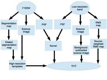
There are several steps for pre-processing both high-resolution and low-resolution images prior to feeding them to TFIT. Figure 8 presents a flow chart of these steps. Galametz et al. (2013) give a detailed description of each step. Here we only summarize some key steps:
-
1.
High-resolution templates: For each source detected in our F160W mosaic, we cut out a postage stamp for it as the high-resolution template. The size of the postage stamp is dependent on the segmentation area generated by SExtractor. This segmentation area of a source, however, only contains pixels above the isophotal detection threshold and could result in an artificial truncation of the light profile of the object. Galametz et al. (2013) determined an empirical relation to extend the segmentation area of an F160W source to a proper size to include the outer wings of an object in the template. This process, called “dilation”, was thoroughly tested and optimized by Galametz et al. (2013).
-
2.
Convolution kernel: TFIT requires a convolution kernel to smooth the high-resolution templates to low-resolution. We use the IRAF/PSFMATCH package to compute the kernel for ground-based bands (CTIO U, VIMOS U, and ISAAC Ks). Our F160W PSF is a hybrid of the empirical PSF from stacking stars and the simulated PSF from TinyTim (van der Wel et al., 2012). Our ground-based low-resolution PSFs and IRAC 3.6 and 4.5 m PSFs are generated by stacking stars, and IRAC 5.8 and 8.0 m PSFs are model PSFs convolved with an empirical kernel to slightly broaden them. For IRAC channels, with FWHMs more than ten times broader than that of F160W, we simply use the IRAC PSFs as kernels to smooth the F160W templates.
-
3.
Low-resolution images: In principle, TFIT can fit both background and objects simultaneously. However, we choose to subtract the background of low-resolution images before running TFIT because fitting background would introduce strong degeneracy and large uncertainty to the photometry of faint sources. Galametz et al. (2013) give details of our background subtraction algorithm. We also run the “empty block” test described in Sec. 3.3 to examine the noise properties of the low-resolution images. In order to correct the effect of the pixel-to-pixel correlations induced by the image reduction, we re-scale the RMS map of each band so that the ratio of the background RMS of the block summed image and the median of the square root of the block summed variance map is equal to unity at block sizes that are close to the typical sizes of sources in the image.
-
4.
Special treatment for individual bands: Several low-resolution bands need special treatment. For both the CTIO/MOSAIC and VLT/VIMOS U-bands, if a source is covered by our ACS F435W image, we use the ACS F435W instead of the WFC3 F160W image as the high-resolution template to minimize the effect of morphological change from the UV to NIR wavelengths. To keep the same detection sources, we still use the dilated F160W segmentation map for creating high-resolution postage stamps. About 2300 sources (7% of our catalog) are not covered by the ACS F435W image. For them, the F160W image is used as the template for both U-bands. For VLT/ISAAC Ks-band, we run TFIT on each of its tiles instead of on the co-added mosaic because the tile-by-tile variation of PSF is non-negligible. We also run TFIT for each epoch of IRAC 5.8 and 8.0 m due to the PSF variation. For sources that are fitted more than once in the ISAAC and IRAC bands, we calculate a weight-averaged flux from each fitting using the squared fitting uncertainty as the inverse weight.
To correct the geometric distortion and/or mis-registration between the high- and low-resolution images, we run TFIT in two passes. In the first pass, TFIT calculates a cross-correlation between the model image and the low-resolution image to determine the optimal shifted transfer kernels for each zone in the image. The second pass then uses these shifted kernels to smooth the high-resolution templates to the low resolution. The two-pass scheme effectively reduces the mis-alignment between templates and low-resolution images.
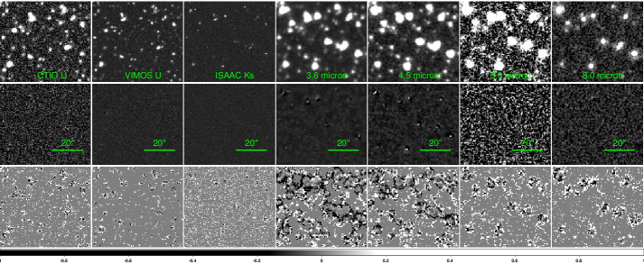
An example of the original images and residual maps of some TFITed bands is shown in Figure 9. A simple visual comparison between the original and the residual images suggests that TFIT does an excellent job of extracting light for the majority of sources in the low-resolution bands. The overall residual is quite close to zero in the maps of U, Ks, and IRAC 5.8 and 8.0 m. Some (especially bright) objects have obvious residuals left in the map of IRAC 3.6 and 4.5 m. To quantify the residual, we calculate the fraction of light left in the residual maps (bottom panels). For most pixels in the sources with the worst residuals, the residual light is around 10% of the original signal. The average residual over the area of these sources, taking into account both positive and negative pixels, is actually quite close to zero, suggesting that the photometry of bright sources in IRAC 3.6 and 4.5 m is not significantly mis-measured, even though their residual maps look worse than others. The residual maps only provide a rough estimate of the quality of our photometry. A quantitative analysis on the quality of the catalog will be presented in Sec. 5.
After measuring the low-resolution photometry with TFIT, we merge the photometry of all the available bands, both low-resolution and HST, into the final catalog. This step is straightforward because each source keeps its ID and coordinates as determined in the F160W detection through the whole procedure of measuring its multi-band photometry. For each source, we also include a weight in each band. For HST and Spitzer bands, the weight is the mean exposure time within six pixels from the center of the object. For other bands, it is the average weight within six pixels from the center. The column descriptions of the catalog are given in Table 5.
5. Quality Checks
We test the quality of our catalog by: (1) comparing colors of stars in our catalog and that in stellar libraries, (2) comparing our catalog with other published catalogs in GOODS-S, (3) measuring zeropoint offsets through the best-fit templates of the SED of spectroscopically observed galaxies, and (4) evaluating the accuracy of photometric redshifts (photo-zs) measured with our catalog.
5.1. Colors of Stars
We first check the quality of our HST photometry by comparing the ACS–WFC3 colors of stars in our catalog with that of stars in stellar libraries. Because GOODS-S is located at high Galactic latitude, a large fraction of its stars may be metal-poor halo stars. The ACS–WFC3 colors, namely, the optical–NIR colors, of stars strongly depend on the metallicity of the stars because the optical fluxes are heavily absorbed by metals while the NIR fluxes are much less affected. Therefore, the ACS–WFC3 colors of stars in GOODS-S may be systematically different from the colors of stars in some commonly used stellar libraries, which are mainly calibrated with bright disk stars with richer metallicity. We use the model of stellar population synthesis of our Milky Way of Robin et al. (2003)111http://model.obs-besancon.fr to estimate the metallicity distribution of stars in GOODS-S and find a median value of [Fe/H]-0.5. We then choose the set of models with metallicity [M/H]=-0.5 from the synthesis stellar library of Lejeune et al. (1997) as our standard reference of stellar colors.
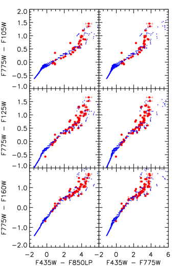
Figure 10 shows the locations of stars in our catalog and those in the Lejuene library in ACS–WFC3 color-color diagrams. Stars are selected with the SExtractor parameter CLASS_STAR0.98 in the F160W band. For each color, we only use stars with S/N3 in the two bands used to calculate the color. If the stellar photometry of one WFC3 band (denoted by X) is incorrectly measured, the (F775W–X) color of observed stars would deviate vertically from that of library stars in both (F775W–X) vs. (F435W–F850LP) and (F775W–X) vs. (F435W–F775W) diagrams by a similar amount. In another situation, if the photometry of one of the ACS Biz bands is mis-measured, the observed stellar color would deviate horizontally by a similar amount from that of library stars in all diagrams of (F775W–X) vs. ACS color, where the ACS color involves the problematic band. There is excellent agreement between our observed stars and library stars for all colors in the plot, suggesting that our stellar ACS–WFC3 colors are accurate.
5.2. Comparison with Other Catalogs
We also compare our photometry with other published multi-wavelength catalogs in GOODS-S. The comparison helps in two ways. First, it provides an assessment of the photometry of extended sources. Second, although we find no systematic offset in our stellar ACS–WFC3 colors, we still need an absolute measurement of the fluxes of either ACS or WFC3 bands.
Two multi-wavelength catalogs in the literature cover (almost) the entire GOODS-S field as well as include most of our bands: GOODS-MUSIC (GM, Grazian et al., 2006; Santini et al., 2009) and FIREWORKS (FW, Wuyts et al., 2008). GM includes ACS F435W, F606W, F775W, and F850LP images, VLT JHKs data, Spitzer/IRAC (3.6, 4.5, 5.8 and 8.0 m) and MIPS (24 m) data, and publicly available U-band data from the ESO 2.2-meter telescope and VLT/VIMOS. A software package, ConvPhot, which operates on the same principle as TFIT, but is a completely independent implementation, has been developed for measuring PSF-matching photometry for space and ground-based images of different resolutions and depths. Different from our detection scheme, GM detects objects mainly in F850LP and is supplemented by Ks- and 4.5 m-band detected sources.
FW is a Ks-selected catalog for the CDF-S, containing photometry in the ACS F435W, F606W, F775W, and F850LP, ground-based U, B, V, R, and I, VLT J, H, and Ks, IRAC 3.6, 4.5, 5.8, and 8.0 m, and MIPS 24 m bands. Photometry in ACS and ISAAC bands is measured using SExtractor in dual-image mode with the Ks-band mosaic as the detection image. Color and aperture photometry are measured with the same apertures in each band. SExtractor MAG_AUTO is used to derive the total flux of the Ks-detected objects. An aperture correction is applied to compute the total integrated flux based on the curve of growth of the PSF of the Ks-band. The total-to-aperture correction factor of the Ks band is then applied to the other ACS and ISAAC bands. Photometry in IRAC bands is measured with the method of Labbé et al. (2006). Similar to TFIT, it fits the light profile of the higher resolution image to that of lower resolution images and leaves flux as a free parameter. For a single source, however, the method does not use the best-fit flux as the total flux of the source. Instead, it subtracts its neighbors based on the best-fit models and then estimates the flux of the source of interest via aperture photometry.
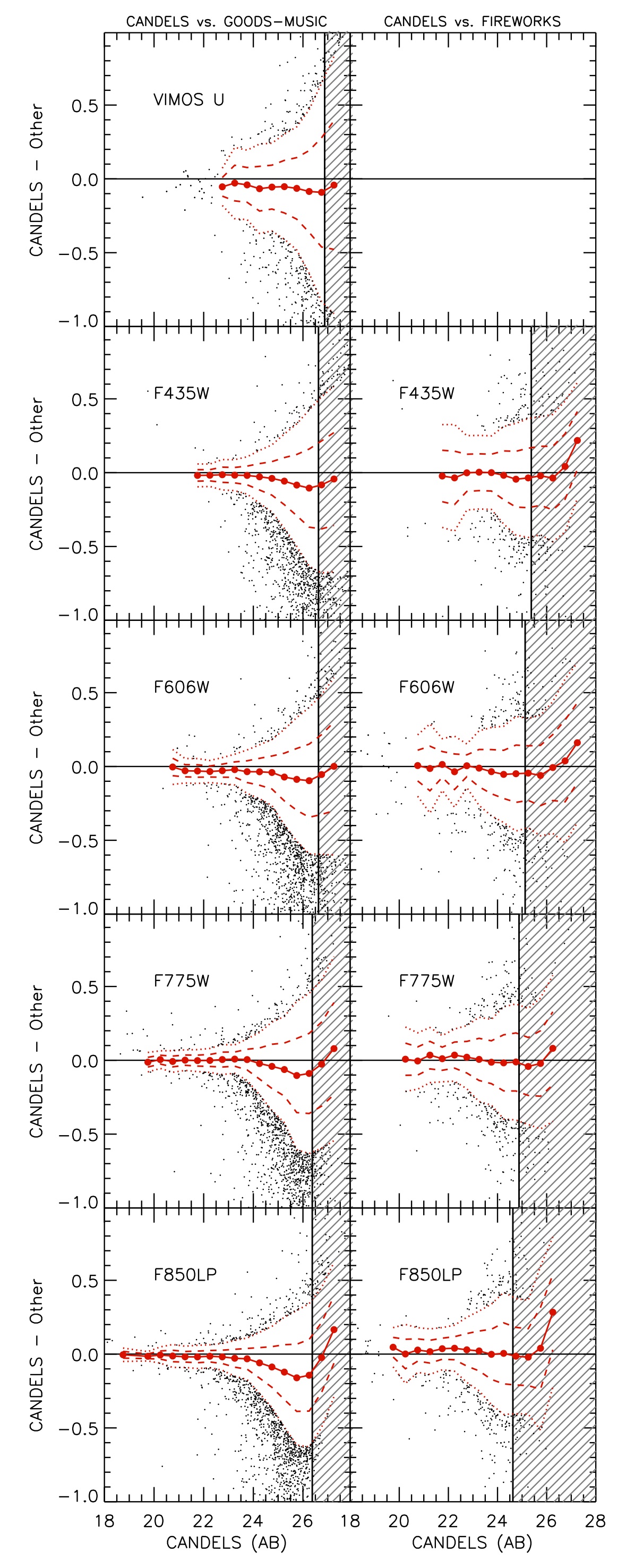
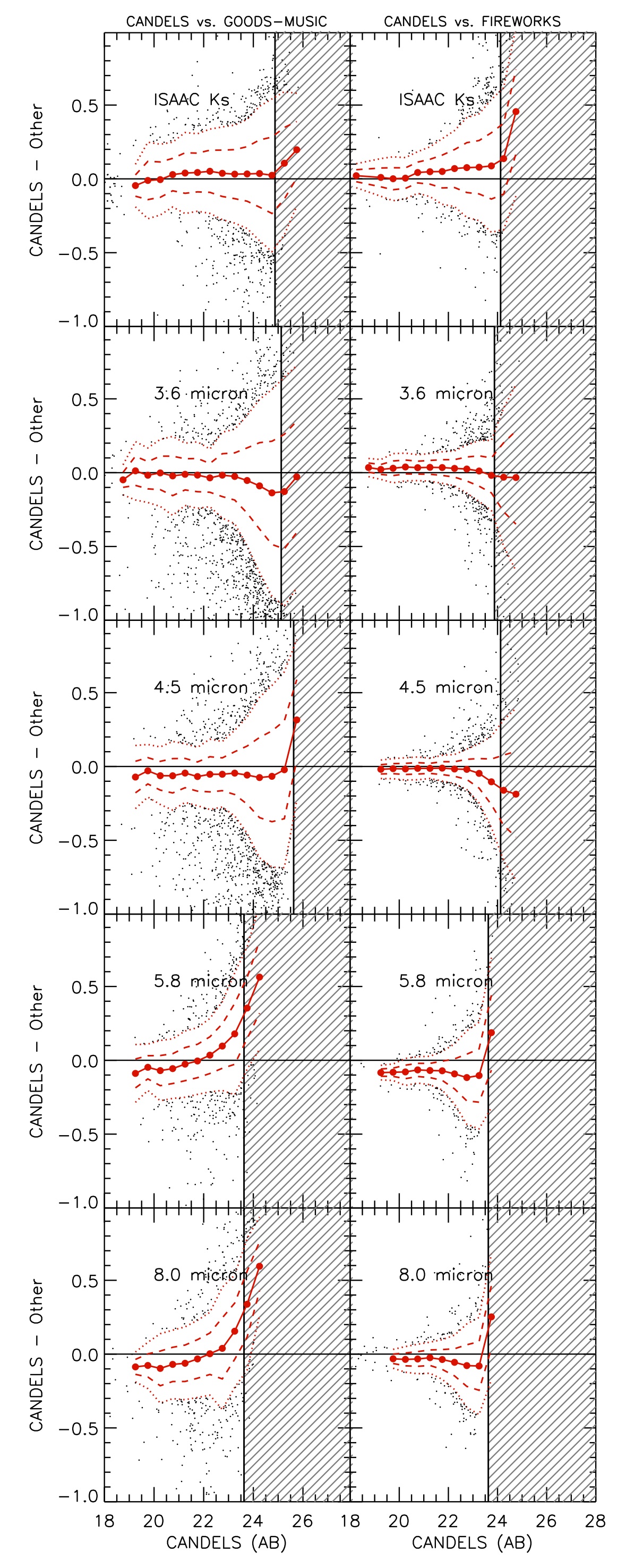
In order to compare our photometry with that in the two catalogs, we match our CANDELS GOODS-S catalog (CGS) to the other two through source coordinates with a maximum matching radius of 03 and 05 for GM and FW, respectively. We only use cleanly detected sources (i.e., not saturated, not truncated, not having bad pixels, etc.) in our catalog with the F160W SExtractor parameter FLAG=0. The comparisons are shown in Figure 11. For each band, we only consider objects with S/N3 in our and the other catalogs.
On average, there is a good agreement with nearly zero systematic offset between CGS and the other two catalogs over the magnitude range to 24 AB mag in most bands (except the IRAC 5.8 and 8.0 m). The offset reaches 0.05 mag in the worst bands. At the faint end ( 24 AB mag), deviations are evident between CGS and the other two.
At the very faint end (the shaded areas in Figure 11), the Eddington bias makes the comparison unreliable. The flux uncertainties of objects in a shallower catalog (GM and FW) are larger so that objects in it are more likely to be scattered to brighter or fainter magnitudes than in a deeper catalog. Sources close to the S/N=3 limit in CGS should be included in the comparison. In fact, however, if the fluxes of their counterparts in GM or FW are scattered toward fainter fluxes, these sources are excluded because their S/N in GM or FW is now 3. Therefore, at the S/N limit, only those CGS sources whose GM and FW fluxes are scattered toward brighter fluxes are included in the comparison. This biases the comparison. In order to determine the magnitude range subjected to Eddington bias in each band, we fit a power law to the differential number count density of GM and FW without any S/N cut. After the S/N3 cut being applied, magnitude ranges where the new differential number count density is less than 50% of the best-fit power law are now very incomplete in GM and FW and hence induce Eddington bias. The comparisons in these magnitude ranges are not discussed here because they are unreliable.
Finally, all comparisons in this section only show the consistency/inconsistency between our and the other two catalogs. They cannot tell us whether one catalog is more accurate than the others.
5.2.1 UV to Optical Photometry
There is an almost constant offset of -0.05 mag between CGS and GM in the VIMOS U-band to 27 AB mag, where CGS measures brighter magnitudes. This deviation could be caused by the different high-resolution templates and kernels used in the template profile fitting method of both catalogs. In GM, ACS F850LP images are used as the templates to fit the U-band image, while in CGS, ACS F435W images are used to minimize the morphological changes along with wavelength. To provide an independent check, we compare our CGS photometry with the SExtractor MAG_AUTO photometry of Nonino et al. (2009). We find good agreement with almost zero offset over the magnitude range to 27 AB mag.
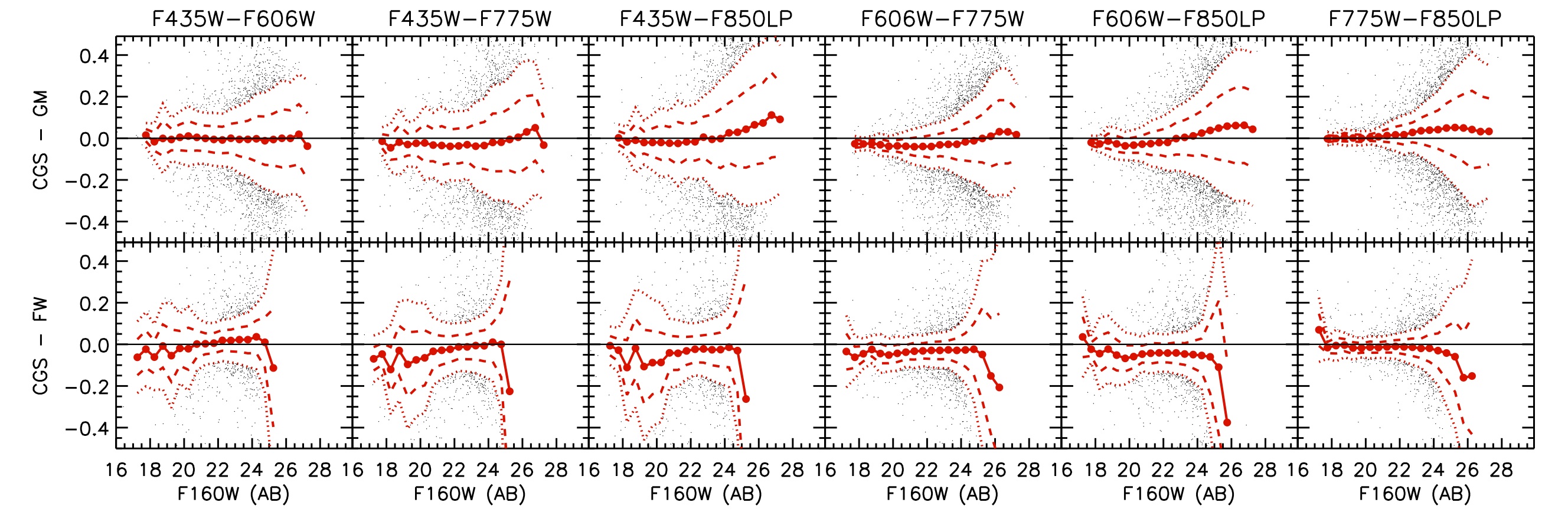
In the ACS bands, the agreement between our and the other two catalogs is quite good. The offset between CGS and GM is almost zero for objects with magnitude brighter than 24 AB mag. The largest offset, seen in the ACS F606W band, is about -0.02 mag. For objects fainter than 24 AB mag, CGS magnitudes are brighter, and the deviation between the two catalogs increases toward fainter magnitude. The deviation may be due to different apertures used to measure the total fluxes in CGS and GM. The aperture size, represented by the KRON_RADIUS in SExtractor, is defined in the F160W band in CGS and then applied to other HST bands through our aperture correction factors, assuming no morphological changes between these bands. In GM, however, the KRON_RADIUS is defined in the ACS F850LP band. Due to the high sensitivity and broader PSF of WFC3, the KRON_RADIUS defined in the F160W band is typically larger than that defined in the F850LP band for each individual source. Therefore, the F160W KRON_RADIUS counts more light from the wings of each object and measures a brighter magnitude. In fact, we find an obvious correlation between the difference of magnitudes and the difference of KRON_RADIUS. Objects whose F160W KRON_RADIUS is larger than the F850LP one are also brighter in our catalog, and vice versa. This correlation supports our speculation that KRON_RADIUS defined in different images is the reason for the deviation in the faint end between CGS and GM. More supportive evidence is from the excellent agreement between the ACS colors of CGS and GM (the upper panels of Figure 12). Colors from both catalogs have almost zero (0.02 mag in the worst case for sources brighter than 26 AB mag in F160W) offset over the magnitude range to F160W 26 AB mag. This excellent agreement demonstrates that our PSF matching process does not induce a systematic offset to our ACS photometry. Therefore, the offset in the faint end of ACS photometry between the two catalogs is likely caused by the different apertures used to measure fluxes.
The comparison between CGS and FW shows large scatter, possibly due to both small number statistics and different photometry measurements. FW has a faint limit cut on 24.3 AB mag in its detection Ks band, which excludes the majority of sources fainter than 25 AB mag in the ACS bands in our catalog. Therefore, the comparison fainter than 25 AB mag has large uncertainty due to small number statistics. Also, FW was generated based on an early version of the GOODS-S ISAAC Ks-band image, which covers 130 arcmin2, only 75% of the whole GOODS-S region. The smaller sky coverage further reduces the number of matched sources in this comparison. For sources brighter than 26 AB, the comparison has larger scatter, 0.15–0.2, than that in the CGS vs. GM comparison. The large scatter is likely due to the treatment of isolated sources and blended sources in the Ks-band in FW. For isolated sources, FW used MAG_AUTO as the total flux with KRON_RADIUS defined in Ks-band. Because the KRON_RADIUS defined in the Ks-band is typically larger than that defined in the HST bands, isolated sources tend to have brighter magnitudes in FW than in CGS. On the other side, to reduce the influence of neighboring sources, FW used a reduction factor to shrink the isophotal area of blended sources and used the isophotal flux to derive the total flux. Therefore, the fluxes of blended sources are likely underestimated in FW. The combination of the above two introduces large scatter to our comparison, as the plot shows. But overall, the mean difference between FW and CGS is close to zero over the magnitude range to 25 AB mag, where the Eddington bias begins to affect the comparison.
5.2.2 IR Photometry
In the ISAAC Ks-band, CGS shows a magnitude-dependent deviation from both GM and FW. CGS becomes fainter than the other two at 20 AB mag. The deviation increases as the flux of sources decreases. At 24 AB mag, the deviation reaches to 0.05 mag in CGS vs. GM and 0.1 mag in CGS vs. FW. Due to the lack of sources with S/N5 at magnitude fainter than 24 AB mag, the deviation in the very faint end cannot be investigated. The deviation could be due to over-subtraction of background in the ISAAC images during our pre-processing of images (Sec. 4). However, measuring global background from the images used by TFIT shows no significant negative background, suggesting that our background subtraction pipeline does a fairly good job. The deviation in CGS vs. FW could also be due to the under-deblending of neighboring sources in SExtractor-type photometry. Contaminating light from poorly separated companions would boost the photometry of faint sources but have little effect on bright sources.
CGS shows good agreement with GM and FW over the magnitude range to 24 AB mag in IRAC 3.6 and 4.5 m. The deviation between CGS and GM is almost zero at 3.6 m and about -0.04 mag at 4.5 m, while that between CGS and FW is about 0.03 mag at 3.6 m and almost zero at 4.5 m. The absolute uncertainty in the IRAC calibration is about 3%. Therefore, we believe that within the calibration uncertainty, there is no major concern on our photometry in the magnitude range of 18–24 AB mag for the IRAC 3.6 and 4.5 m.
The comparison in the IRAC 5.8 and 8.0 m can only be done for sources brighter than 23 AB mag. The deviations between CGS and GM in both channels are quite similar and magnitude dependent. CGS is brighter than GM by 0.1 mag at 19 AB mag and becomes fainter than GM by 0.05 mag at 23 AB mag. In contrast, the deviations between CGS and FW are almost constant, with CGS being brighter by 0.07 mag and 0.03 mag in the 5.8 and 8.0 m bands, respectively.
Although all three catalogs use the profile template fitting method to derive the photometry of IRAC bands, the implementation of this method in each catalog is quite different. The scatter in CGS vs. FW is significantly smaller than that in CGS vs. GM. We suspect that the difference in scatter originates from the choice of high-resolution templates. NIR images are used in both CGS (F160W) and FW (Ks-band) as the templates for fitting IRAC images. Although the resolution differs between the two sets of templates, the morphological change from them to IRAC bands would be quite small. On the other side, GM uses the ACS z-band as templates to fit the profile of sources in IRAC bands. Since the templates and the IRAC images sample two distinct wavelength regimes, the morphological change could induce large difference in photometry, including systematic offset in the 5.8 and 8.0 m bands, where the wavelength difference between templates and sources becomes the largest.
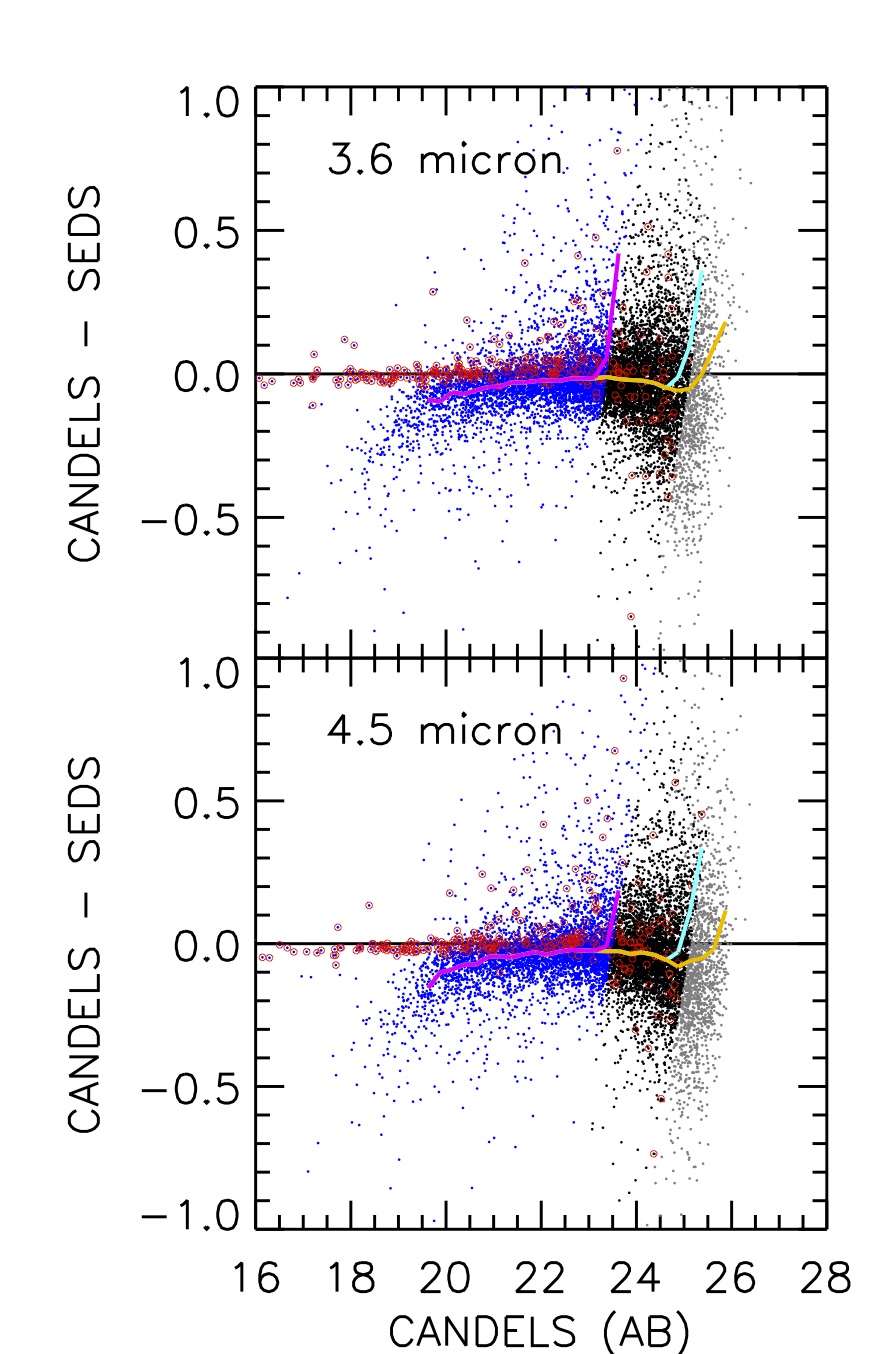
We also compare our TFIT photometry to the official SEDS catalog (Ashby et al., 2013) for IRAC 3.6 and 4.5 m bands. Ashby et al. used StarFinder to fit PSFs to sources and subtracted the best-fit PSFs from the original image. Then, for each source, they added its best-fit PSF back to the residual map while keeping other sources subtracted. They measured aperture photometry for the source with a variety of aperture sizes (here we choose the one with size of 24) and applied a correction factor to convert the aperture photometry to the total photometry based on the curve of growth of the IRAC PSFs. The comparison of CANDELS TFIT photometry and SEDS photometry is shown in Figure 13. For point-like sources (F160W SExtractor parameter CLASS_STAR0.8) in both IRAC channels, the agreement between both catalogs is excellent over the magnitude range to 24.5 AB mag with an offset of -0.04 mag. For bright (20 AB mag) extended sources, however, SEDS underestimates their fluxes. This is because the aperture correction used in SEDS is only valid for point sources. When using larger apertures (e.g., size of 60), SEDS photometry of bright extended sources agrees with our TFIT photometry much better with deviation 0.05 mag. Ashby et al. (2013) give a detailed description and analysis of SEDS photometry and its uncertainty.
Figure 12 also illustrates the Eddington bias in comparing two catalogs. Sources near the threshold will randomly have greater S/N in one catalog than the other. Imposing a S/N cutoff means that sources just above the cutoff will on average have catalog fluxes that are larger than the true values. If the uncertainties of the two catalogs differ, the amount of bias will differ. This effect can be seen in the figure as the sloping transition from blue (S/N8) to black (S/N5) and from black (S/N5) to gray (S/N3) points. The deviation of 0.05 mag at 23.5 AB mag for curves with S/N8 is strongly biased and hence does not suggest any true difference between the two catalogs at this magnitude. In fact, good agreement between the two catalogs can be seen down to 25.5 AB mag where the S/N3 cut induces the Eddington bias.
Due to the Eddington bias, it is difficult to evaluate the accuracy of our IRAC photometry at the very faint end through comparisons with other catalogs. Instead, we use fake source simulations to test our photometry at the detection limit of the IRAC channels. We generate 1000 fake F160W sources and place them randomly into our F160W mosaic. We then use our TFIT pipeline to measure the IRAC photometry of these fake sources and real sources simultaneously. Because there are no counterparts of these fake sources in IRAC images, on average their IRAC photometry should be zero. Indeed, the distributions of the ratio of IRAC photometry and its uncertainties of these fake sources in all IRAC channels have a mean of zero and a standard deviation of one. This result demonstrates that – assuming no PSF or registration mismatches – our catalog accurately measures IRAC photometry and its uncertainties down to the detection limits of IRAC images.
5.3. Zeropoint Offsets
To further assess the overall accuracy of our photometry and its influence on deriving properties of galaxies, we measure the zeropoint offset of each band by comparing the SEDs of spectroscopically observed galaxies to synthetic stellar population models. If a band suffers from significant systematic bias, its photometry will statistically deviate from the best-fit models.
The spectroscopic sample used in our study is from Dahlen et al. (2010). We match the sample to our F160W band coordinates with a maximum matching radius of 03. We only use galaxies with good (flag=1 in Dahlen et al., 2010) spectroscopic redshifts (spec-zs) and exclude X-ray detected sources. The sample contains 1338 galaxies. The synthetic stellar population models used in this test are retrieved from the PEGASE v2.0 library (Fioc & Rocca-Volmerange, 1997). Details of SED-fitting can be found in Guo et al. (2012). For each galaxy, we fix its redshift to its spec-z during the fitting.
| Band | Zeropoint Offset111Offsets are defined as observed magnitude minus model magnitude. A positive offset means our photometry is fainter than models, and vice versa. | Zeropoint Offset |
|---|---|---|
| (Before Template Correction) | (After Template Correction) | |
| U_CTIO | ||
| U_VIMOS | ||
| F435W | ||
| F606W | ||
| F775W | ||
| F814W | ||
| F850LP | ||
| F098M | ||
| F105W | ||
| F125W | ||
| F160W | ||
| ISAAC Ks | ||
| HAWK-I Ks | ||
| IRAC 3.6m | ||
| IRAC 4.5m | ||
| IRAC 5.8m | ||
| IRAC 8.0m |
The template fitting can suffer from systematic errors if the models do not match real galaxy SEDs or if the absolute calibrations of the observations are systematically wrong at different wavelengths. In order to correct for such errors, we shift the observed and best-fit SEDs of each galaxy to rest-frame wavelength and calculate the offset between them as a function of rest-frame wavelength. The average offset of the spec-z sample at a given rest-frame wavelength is thus contributed by multiple bands that observe galaxies at different redshifts. Therefore, any offset found in such a way is likely due to the inaccuracy of the SED templates instead of the systematic errors of our photometry, unless all the bands contributing to the rest-frame wavelength underestimate/overestimate fluxes in the same direction. We then subtract the offsets at all rest-frame wavelengths from our SED templates.
The zeropoint offsets of all bands are shown in Table 3, both before and after applying the template correction. For most non-IRAC bands, the offset is 0.02 mag. The only non-IRAC band with significant offset is ISAAC Ks-band, whose offset is 0.06 mag. For IRAC 3.6, 4.5, and 5.8 m, the offsets are reduced by the template correction to 0.05 mag. This value is consistent with the deviation between different measurements from our previous comparisons with other catalogs. The offset of IRAC 8.0 m is quite large, though. For galaxies at z0.4 (about 20% of our spec-z galaxies), this band is affected by the emissions of polycyclic aromatic hydrocarbon (PAH). The PAH emissions are not characterized in our SED models even after our correction, and thus the observed IRAC 8.0 m flux should be much brighter than the SED templates.
| All | z1.5 | z1.5 | ||||||||||
|---|---|---|---|---|---|---|---|---|---|---|---|---|
| mean | NMAD | mean | NMAD | mean | NMAD | |||||||
| All (before template correction) | 0.010 | 0.040 | 6.1% | 0.031 | 0.013 | 0.042 | 6.9% | 0.035 | 0.001 | 0.035 | 3.5% | 0.023 |
| (after template correction) | -0.002 | 0.037 | 5.5% | 0.028 | -0.003 | 0.037 | 6.0% | 0.030 | -0.001 | 0.037 | 3.8% | 0.023 |
| H24 AB (before template correction) | 0.012 | 0.041 | 5.3% | 0.032 | 0.013 | 0.042 | 5.8% | 0.034 | 0.004 | 0.037 | 3.0% | 0.023 |
| (after template correction) | -0.002 | 0.037 | 4.8% | 0.028 | -0.003 | 0.037 | 5.1% | 0.029 | 0.002 | 0.039 | 3.6% | 0.024 |
| H24 AB (before template correction) | -0.001 | 0.039 | 11.7% | 0.029 | 0.009 | 0.050 | 22.2% | 0.057 | -0.006 | 0.031 | 4.4% | 0.022 |
| (after template correction) | -0.004 | 0.036 | 10.3% | 0.027 | 0.001 | 0.043 | 19.0% | 0.046 | -0.008 | 0.030 | 4.4% | 0.021 |
Overall, the systematic offset in our catalog is small (0.02 mag) for most UV-to-NIR bands and modest (0.05 mag) for ISAAC Ks and IRAC 3.6, 4.5, and 5.8 m. IRAC 8.0 m suffers from large systematic offsets, possibly due to PAH emissions. These derived zeropoint offsets depend on both the redshift distribution of the spec-z training sample and the choice of the photo-z templates. Therefore, they can only serve as a rough evaluation of the quality of our catalog. We do not apply these offsets to our catalog.
5.4. Photometric Redshifts
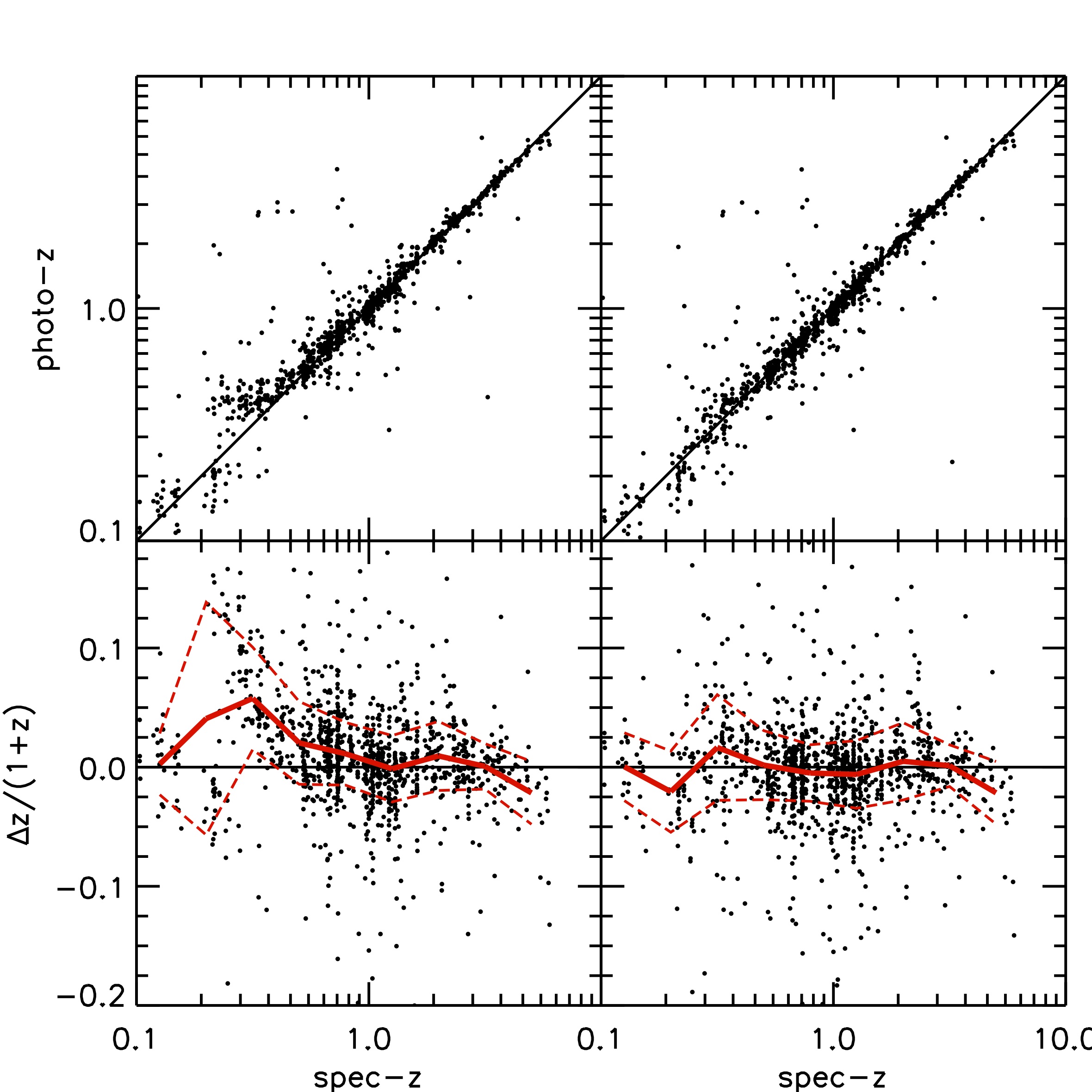
We now measure photometric redshifts (photo-zs) of galaxies in our spectroscopic sample. We use the PEGASE v2.0 templates, both before and after applying our template correction to them. The accuracy of our photo-z measurement is shown in Figure 14, and detailed statistics on the accuracy are listed in Table 4. Our template correction mainly affects objects at z1 and corrects the systematic overestimate of photo-z among them. After the template correction, our measurement has the normalized median absolute deviation (NMAD, defined as ) of 0.028 and an outlier fraction (defined as ) of 5.5% for all galaxies. These values are slightly better for bright (H24 AB) galaxies, but worse for faint (H24 AB) objects.
For galaxies at z1.5, the accuracy increases to an NMAD0.023 and outlier fraction of 4.0%, regardless of whether template correction is applied or not. The accuracy also depends little on the brightness of objects. This high accuracy indicates the importance of the CANDELS NIR data on photo-z measurement for galaxies at intermediate or high redshift. The deep CANDELS photometry in our catalog effectively characterizes the Balmer/4000 Å break for galaxies at z1.5 and hence yields an accurate photo-z measurement for them. For low-redshift (z1.5) galaxies, their photo-zs are determined by both major spectral breaks (Lyman or Balmer) as well as the Rayleigh–Jeans regime of stellar emission. The latter is quantified by IRAC photometry in our catalog, which has larger uncertainty than CANDELS NIR photometry and hence reduces the accuracy of the photo-z of z1.5 galaxies.
It is also possible that the high accuracy of our photo-zs of z1.5 galaxies is due to the narrow range of the spectral types of our spec-z sample, which are fully covered by our SED-fitting templates. The narrow range of the spectral types could be physically real because galaxies at z1.5 have a relatively simple star formation history, or it could be due to the selection bias of our spectroscopically observed sample. On the other side, our templates may not fully cover the spectral types of z1.5 galaxies because of their complicated star formation histories as well as variation in the dust extinction law, resulting in a decreased photo-z accuracy. In order to improve the photo-z at z1.5, the uncertainties of SED-fitting templates in stellar evolutionary track, star formation history, dust extinction law, and spectral features should be taken into account. For example, Brammer et al. (2008) introduced a template error function to incorporate the above uncertainties together with the photometric uncertainty into the template fitting algorithm. The template error function minimized systematic errors in their photo-zs.
Overall, our photo-z measurement shows that our photometric catalog is sufficient to provide accurate photo-zs for galaxies, especially for those at z1.5, where CANDELS NIR data greatly improve the quality of photo-zs. The CANDELS team is working on generating a photo-z catalog for the GOODS-S field (Dahlen et al., 2013, in preparation).
6. Application of the Catalog to Studying Galaxies at z=2–4

6.1. Detection Ability
Because our catalog is constructed based on F160W detection, the depth and completeness of our F160W band place the primary limit on our detection ability. We use galaxy templates drawn from the updated version of Bruzual & Charlot (2003, CB09) to predict the F160W photometry for different types of galaxies. The detection ability of our catalog is plotted in Figure 15. For simplicity, we only discuss galaxies with stellar mass of and age of 1 Gyr at the epoch of observation. Galaxies with a constant star formation history and low dust extinction (e.g., E(B-V)=0.15) can be detected with a completeness of 50% to z3.4 and z4.6 in our wide and deep regions, respectively. Due to their very red rest-frame UV and optical colors, star-forming galaxies with high dust-extinction can only be detected with the same completeness to lower redshift. Galaxies with E(B-V)=0.6 can only be detected to the 50% completeness to z2.0, 2.4 and 3.0 for the wide, deep, and HUDF regions, respectively. For passively-evolving galaxies (PEGs), we can detect them with 50% completeness to z2.8, 3.2, and 4.2 in the wide, deep, and HUDF regions, if they are unreddened. For galaxies with age older than 1 Gyr, the maximum detectable redshift is lower. For example, PEGs with age of 2 Gyr can be detected with a 50% completeness to z=2.4 and 2.8 for the wide and deep regions.

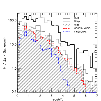
Figure 16 compares the differential number density of our catalog with that of other surveys that contain H-band data: GOODS NICMOS Survey (GNS, Conselice et al., 2011), GOODS-VLT Survey (Retzlaff et al., 2010), and NICMOS HDF Survey (Dickinson et al., 2000; Thompson, 2003). The representative 50% completeness limits of GNS and GOODS-VLT estimated through the best-fit power law are 25.1 and 24.3 AB mag, respectively. Our wide (deep) region is 0.8 (1.5) and 1.6 (2.3) mag deeper than GNS and GOODS-VLT. Therefore, our catalog in the wide (deep) region is able to detect galaxies with stellar mass lower than the minimum detectable stellar mass of GNS and GOODS-VLT by a factor of two (four) and four (eight). The NICMOS HDF Survey is deeper than our deep region but fainter than our HUDF region. However, its small sky coverage, about 1 arcmin2, brings large cosmic variance and small number statistics, as can be inferred from its irregular differential number density distribution.
To further demonstrate the detection ability of our catalog, we compare the overall photo-z distributions of the three regions of our catalog to that of GOODS-MUSIC and FIREWORKS in Figure 17. We cut each region/catalog to its 50% completeness magnitude through the best-fit power law to the differential source number density of each region/catalog, as discussed in Sec. 3.1. This threshold magnitude is F850LP=26.4 AB mag for GOODS-MUSIC and Ks=24.1 for FIREWORKS.
The photo-z distributions of our wide region and GOODS-MUSIC are similar, suggesting a comparable detection ability at all redshifts, although our wide region has a marginal excess of detection ability at z2 and z5. Our deep and HUDF regions surpass the GOODS-MUSIC catalog at all redshifts. The source number density in our deep (HUDF) region is higher than that of GOODS-MUSIC by a factor of 2 (6) at 0z5, and by a factor of () at z5. All our three regions have much higher source number density in each redshift bin than FIREWORKS.
6.2. Balmer Break Selected Galaxies at z2–4
Our deep NIR photometry provides an accurate description of the Balmer/4000 Å break for galaxies at z2–4, and enables selecting high-redshift galaxies through broad-band colors that cover the break. Although current photo-z measurements can achieve a fairly high accuracy, color selection methods still play an important role in selecting high-redshift galaxies. The bias, efficiency, and contamination of color selections can be explicitly determined through Monte Carlo simulation of selecting fake galaxies with various magnitude, size, color, and star-formation history. Color selections are also fast and easy to reproduce.
A popular color-color selection criterion using the Balmer break is the BzK method proposed by Daddi et al. (2004). This method, using the (B-z) and (z-K) colors to quantify the strength and curvature of the Balmer break, is proven successful at selecting star-forming galaxies independent of their dust reddening as well as passively evolving galaxies at z2. However, due to the lack of deep NIR photometry of large fields, extending this method to higher redshifts has not been extensively discussed. It was only extended to galaxies at z3 in the ERS field by Guo et al. (2012) using the (V-J) and (J-3.6m) colors. Our catalog with the deepest NIR photometry in the GOODS-S field is the first one that makes this Balmer break selection method practical in large fields. We apply the two selection criteria to our catalog and also extend them to z4.
The selection criteria used here are as follows.
-
1
Star-forming BzK: , and passively evolving BzK: , where and are F435W and F850LP;
-
2
Star-forming VJL: , and passively evolving VJL: , where , , and are F606W, F125W, and IRAC 3.6 m;
-
3
Star-forming iHM: , and passively evolving iHM: , where , , and are F775W, F160W, and IRAC 4.5 m.
For BzK, we demand S/N5 in the z- and Ks-band. We use the ISAAC Ks-band here because it covers the entire GOODS-S field. Sommariva et al. (2013, in preparation) are studying BzK selected sources in both GOODS-S and UDS based on the HAWK-I Ks-band. For VJL and iHM, we demand S/N10 in the two reddest bands used in each criterion.
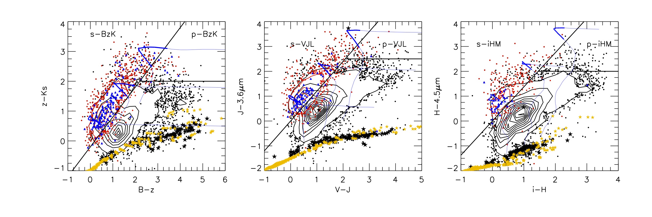
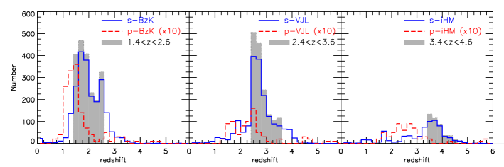
The color–color diagram of each selection criterion is shown in Figure 18. The target redshift range of each criterion is z1.5–2.5 for BzK, 2.5–3.5 for VJL, and 3.5–4.5 for iHM. Galaxies with photo-zs within each target range are over-plotted in each diagram. These selection criteria do a fairly good job at selecting galaxies in their own target redshift range. Figure 19 shows the redshift distribution of selected galaxies in each criterion. We can roughly estimate the effectiveness and contamination of each criterion by comparing the redshift distribution of selected galaxies (blue histogram) and that of total galaxies (black histogram). The effectiveness, defined as the fraction of galaxies in the target redshift range that are selected by a given criterion, is about 86%, 83%, and 83% for BzK, VJL, and iHM, respectively. The contamination, defined as the fraction of selected galaxies that are not within the target redshift range of the selection criterion, is about 21%, 30%, and 50% for BzK, VJL, and iHM, respectively.
We also compare the observed and synthetic stellar locus in the color–color diagrams to examine our NIR photometry. Since our tests on the ACS–WFC3 colors of stars show no offset between the observed and synthetic stars (Sec. 5.1), any deviation between the observed and synthetic stars in these diagrams is caused by the systematic offset of the NIR bands. In the BzK diagram, the colors of observed stars show good agreement with those of stars in the synthetic library of Lejeune et al. (1997), suggesting no systematic offset in our ISAAC Ks-band photometry. In the VJL and iHM diagrams, a mild deviation about 0.05 mag is found between the observed and synthetic stars. This deviation may indicate that our 3.6 and 4.5 m fluxes are overestimated by 0.05 mag. It can also be due to, however, the inaccurate calibration of the NIR regime of the stellar libraries.
Passively evolving galaxies at z3 potentially hold important clues to the processes that quench star-formation in massive galaxies, and to the emergence of the Hubble sequence. As discussed above, our catalog is able to detect such galaxies to z3. Although the redshift distribution of selected passive galaxies (red histograms in Figure 19) declines dramatically at z3, we still find 26 galaxies from the passive selection windows. The major contamination source in the passive selection windows is dusty star-forming galaxies at lower redshift. In order to exclude the contamination, we remove 13 sources with MIPS 24 m detection. If the remaining 13 galaxies are confirmed to have the passive nature, their star formation activity should have ceased at least 0.5–1 Gyrs ago, i.e., at z5.
6.3. Red Galaxies at z2–4
Based on their positions in the color–magnitude diagram (CMD), local galaxies can be roughly divided into two populations: blue cloud and red-sequence (e.g., Strateva et al., 2001; Blanton et al., 2003; Baldry et al., 2004). Galaxies in the blue cloud are reliably classified as spiral galaxies with ongoing star-formation, and their color is strongly related to the recent star-formation history. Galaxies in the red-sequence (except dust-reddened spirials) generally have little recent star-formation. This color bimodality has been reported up to z3 (e.g., Bell et al., 2004; Cassata et al., 2008; Kriek et al., 2009; Brammer et al., 2009; Whitaker et al., 2011). It is unclear, however, at which cosmic epoch this color bimodality emerges, owing to limitations of the accuracy of photo-zs and rest-frame UV–optical colors.
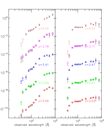
The deep NIR photometry of our catalog provides a unique tool to detect red galaxies at z3 to investigate the origin of the color bimodality. Figure 20 shows the rest-frame color–magnitude diagram of galaxies at different redshifts in our catalog. We use the extrapolation of the red–blue separation line of Bell et al. (2004) to separate the blue cloud and red-sequence. The red-sequence is clearly shown at z2. At 2z3, the red-sequence becomes less obvious, but there is still a large amount of galaxies which are well separated from the blue cloud and enter the red region. At z3, due to the decline of number of galaxies, the separation of the two populations is not as clear as at lower redshifts. However, a handful of galaxies still have red enough rest-frame UV–optical color to enter the red region, suggesting the existence of passive galaxies at z3.
We present a few examples of red and blue SEDs at 3z4 in our catalog in Figure 21 to show the quality of our photometry. The small uncertainties on the rest-frame UV–optical colors enable reliable separation of different types of SEDs of galaxies up to z4. However, although red galaxies at z4 suggest the existence of evolved galaxies with little ongoing star formation at such high redshift, they could also be dusty star-forming galaxies whose rest-frame UV–optical colors are reddened by dust. To investigate the nature, stellar masses, and number densities of these red galaxies is a subject for future works.
| Column No. | Column Title | Description |
|---|---|---|
| 1 | ID | Object identifier, beginning from 1 |
| 2 | IAU Name | |
| 3,4 | RA, DEC | Right ascension and declination (J2000.0; decimal degrees) |
| 5 | F160W Limiting Magnitude | Limiting magnitude at the position of the source in the F160W image111The limiting magnitude here is derived as , where is the average of the squared RMS in the SExtractor F160W segmentation map of each source, is the area of 1 , and is the zero-point of F160W. |
| 6 | FLAGS | SExtractor F160W flag used to designate suspicious sources that fall in contaminated regions222A non-contaminated source has a flag of “0”. Sources detected on star spikes, halos, and the bright stars that produce those spikes and halos have a flag of “1”. Sources detected by SExtractor at the image edges or on the few artifacts of the F160W image are assigned a flag of “2”. Sources with both the flag of “1” and “2” have a flag of “3”. |
| 7 | CLASS_STAR | SExtractor CLASS_STAR parameter in the F160W band |
| 8–58 | Flux, Flux_Err, Weight | Triplet of flux, flux uncertainty, and weight in each filter. Sources that are not observed have (-99.00, -99.00, 0). |
| In HST bands, the weight is the exposure time of the source, while in other bands, it is a relative weight. | ||
| Filters are included in order: CTIO_U, VIMOS_U, F435W, F606W, F775W, F814W, F850LP, F098M, F105W, | ||
| F125W, F160W, ISAAC_Ks, HAWK-I_Ks, 3.6 m, 4.5 m, 5.8 m, and 8.0 m | ||
| 59, 60 | FLUX_ISO, FLUXERR_ISO | F160 isophotal flux and flux error333For sources whose isophotal radius smaller than 2.08 pixels, these parameters are replaced by FLUX_APER and FLUXERR_APER measured within a radius of 0125 (2.08 pixels). See Sec. 3.2 for details. |
| 61, 62 | FLUX_AUTO, FLUXERR_AUTO | F160 AUTO flux and flux error |
| 63 | FWHM_IMAGE | FWHM of the F160W image of object, in unit of pixel (1 pixel = 006) |
| 64, 65 | A_IMAGE, B_IMAGE | F160W profile RMS along major and minor axis (pixel) |
| 66 | KRON_RADIUS | F160W band Kron radius from SExtractor (in unit of A_IMAGE or B_IMAGE) |
| 67, 68, 69 | FLUX_RADIUS | F160W band FLUX_RADIUS with the fraction of light of 0.2, 0.5, and 0.8 from SExtractor (pixel) |
| 70 | THETA_IMAGE | F160W position angle (degree) |
| 71 | Apcorr | Ratio of SExtractor FLUX_AUTO and FLUX_ISO in the F160W band |
| 72 | HOT_FLAG | A flag to designate if the source enters the catalog as detected in the cold mode (=0) or in the hot mode (=1) |
| 73 | ISOAREAF_IMAGE | SExtractor F160W Isophotal area (filtered) above Detection threshold () |
7. Summary
We present a UV-to-mid infrared multi-wavelength catalog in the CANDELS/GOODS-S region, combining the newly obtained CANDELS HST/WFC3 F105W, F125W, and F160W data with existing public data. The catalog is based on source detection in the WFC3 F160W band. To maximize the scientific yields of our catalog, we construct a “max-depth” F160W mosaic, which includes data from the CANDELS deep and wide observations as well as two previous HST/WFC3 programs, ERS and HUDF09. The F160W mosaic, providing the deepest photometry for each individual source in GOODS-S, reaches a 5 limiting depth (within an aperture of 017, the FWHM of the F160W) of 27.4, 28.2, and 29.7 AB mag for CANDELS wide, deep + ERS, and HUDF regions, respectively. The representative 50% completeness of our catalog reaches 25.9, 26.6, and 28.1 AB mag in the F160W band for the three regions. The catalog contains 34930 sources in total.
In addition to WFC3 NIR bands, the catalog also includes data from UV (U-band from both CTIO/MOSAIC and VLT/VIMOS), optical (GOODS HST/ACS F435W, F606W, F775W, F814W, and F850LP), and IR (ERS WFC3 F098M, VLT/ISAAC Ks, VLT/HAWK-I Ks, and Spitzer/IRAC 3.6, 4.5, 5.8, 8.0 m) observations. We use SExtractor to measure photometry for all available HST bands from PSF matched images. For other low-resolution bands, whose FWHMs of PSFs vary by almost a factor of 10, we use our profile template fitting package, TFIT, to measure the uniform photometry among them.
The quality of the multi-wavelength catalog is thoroughly tested. First, the comparison between the ACS–WFC3 colors of stars in our catalog and those of stars in synthetic stellar libraries shows excellent agreements. Second, the difference of photometry between our catalog and GOODS-MUSIC and FIREWORKS is nearly zero over the magnitude range to 24 AB mag, with the worst offset being 0.05 mag. We discuss the possible reasons of the deviations between our and other catalogs at the faint end. Last, the zeropoint offsets measured by comparing the observed SEDs to the best-fit stellar population synthesis templates of spectroscopically observed galaxies are 0.02 mag for most UV-to-NIR bands. The photo-zs measured with our catalog can reach the accuracy of NMAD0.028.
Our catalog is able to detect star-forming galaxies with stellar mass of to z3.4, 4.6, and 8.0 at a 50% completeness in the wide, deep, and ultra-deep regions, respectively. Passive galaxies with the same stellar mass can be detected at a 50% completeness to z2.8, 3.2, and 4.2 in above regions. Our catalog in the wide and deep regions is about 1–2 mag deeper than other public H-band surveys. The minimum detectable stellar mass in the wide and deep regions of our catalog is therefore smaller than that of other H-band surveys by a factor of about 3–6.
To provide an example of applying our catalog to study distant galaxies, we use color criteria to select both star-forming and passively evolving galaxies at z=2–4 through the strength and curvature of the Balmer Break. We examine the redshift distribution of selected galaxies and discuss the effectiveness and contamination of the selection criteria. The detection of red galaxies with obvious Balmer break in our catalog suggests the existence of passive galaxies at z3.
We also study the evolution of the rest-frame color–magnitude diagram, (U-V) vs. , from z=0 to z=4 to investigate the emergence of the color bimodality in the universe. A handful of red galaxies, possibly a combination of passive galaxies and dusty star-forming galaxies, are detected in our catalog at z4.
The CANDELS GOODS-S multi-wavelength catalog and its associated files are
publicly available on the CANDELS website, in the Mikulski Archive for Space
Telescopes (MAST), via the on-line version of the article, and the Centre de
Donnees astronomiques de Strasbourg (CDS) as well as in the Rainbow
Database.
We thank the anonymous referee for constructive comments that improve this article. Support for program number HST-GO-12060 was provided by NASA through a grant from the Space Telescope Science Institute, which is operated by the Association of Universities for Research in Astronomy, Incorporated, under NASA contract NAS5-26555. YG and the authors from UCSC acknowledge support from NASA HST grant GO-12060.10-A and NSF grant AST-0808133. JSD acknowledges the support of the European Research Council via the award of an Advanced Grant and the support of the Royal Society via a Wolfson Research Merit Award. This work is based in part on observations made with the Spitzer Space Telescope, which is operated by the Jet Propulsion Laboratory, California Institute of Technology under a contract with NASA. Support for this work was provided by NASA through an award issued by JPL/Caltech.
Facilities: HST (ACS and WFC3) and Spitzer (IRAC)
References
- Ashby et al. (2013) Ashby, M. L. N., Willner, S. P., Fazio, G. G., et al. 2013, ApJ, 769, 80
- Baldry et al. (2004) Baldry, I. K., Glazebrook, K., Brinkmann, J., et al. 2004, ApJ, 600, 681
- Balestra et al. (2010) Balestra, I., Mainieri, V., Popesso, P., et al. 2010, A&A, 512, A12
- Barden et al. (2012) Barden, M., Häußler, B., Peng, C. Y., McIntosh, D. H., & Guo, Y. 2012, MNRAS, 422, 449
- Barro et al. (2011) Barro, G., Pérez-González, P. G., Gallego, J., et al. 2011, ApJS, 193, 13
- Bell et al. (2004) Bell, E. F., Wolf, C., Meisenheimer, K., et al. 2004, ApJ, 608, 752
- Blanton et al. (2003) Blanton, M. R., Hogg, D. W., Bahcall, N. A., et al. 2003, ApJ, 594, 186
- Bouwens et al. (2009) Bouwens, R. J., Illingworth, G. D., Franx, M., et al. 2009, ApJ, 705, 936
- Bouwens et al. (2010a) Bouwens, R. J., Illingworth, G. D., Oesch, P. A., et al. 2010a, ApJ, 709, L133
- Bouwens et al. (2010b) Bouwens, R. J., Illingworth, G. D., Oesch, P. A., et al. 2010b, ApJ, 708, L69
- Bouwens et al. (2012) Bouwens, R. J., Illingworth, G. D., Oesch, P. A., et al. 2012, ApJ, 752, L5
- Brammer et al. (2008) Brammer, G. B., van Dokkum, P. G., & Coppi, P. 2008, ApJ, 686, 1503
- Brammer et al. (2009) Brammer, G. B., Whitaker, K. E., van Dokkum, P. G., et al. 2009, ApJ, 706, L173
- Bruzual & Charlot (2003) Bruzual, G., & Charlot, S. 2003, MNRAS, 344, 1000
- Casertano et al. (2000) Casertano, S., de Mello, D., Dickinson, M., et al. 2000, AJ, 120, 2747
- Cassata et al. (2008) Cassata, P., Cimatti, A., Kurk, J., et al. 2008, A&A, 483, L39
- Cimatti et al. (2008) Cimatti, A., Cassata, P., Pozzetti, L., et al. 2008, A&A, 482, 21
- Coe et al. (2013) Coe, D., Zitrin, A., Carrasco, M., et al. 2013, ApJ, 762, 32
- Conselice et al. (2011) Conselice, C. J., Bluck, A. F. L., Buitrago, F., et al. 2011, MNRAS, 413, 80
- Daddi et al. (2004) Daddi, E., Cimatti, A., Renzini, A., et al. 2004, ApJ, 617, 746
- Daddi et al. (2007) Daddi, E., Dickinson, M., Morrison, G., et al. 2007, ApJ, 670, 156
- Dahlen et al. (2010) Dahlen, T., Mobasher, B., Dickinson, M., et al. 2010, ApJ, 724, 425
- Dickinson et al. (2000) Dickinson, M., Hanley, C., Elston, R., et al. 2000, ApJ, 531, 624
- Dunlop et al. (2012) Dunlop, J. S., McLure, R. J., Robertson, B. E., et al. 2012, MNRAS, 420, 901
- Fazio et al. (2004) Fazio, G. G., Hora, J. L., Allen, L. E., et al. 2004, ApJS, 154, 10
- Finkelstein et al. (2010) Finkelstein, S. L., Papovich, C., Giavalisco, M., et al. 2010, ApJ, 719, 1250
- Finkelstein et al. (2012a) Finkelstein, S. L., Papovich, C., Ryan, R. E., et al. 2012a, ApJ, 758, 93
- Finkelstein et al. (2012b) Finkelstein, S. L., Papovich, C., Salmon, B., et al. 2012b, ApJ, 756, 164
- Fioc & Rocca-Volmerange (1997) Fioc, M., & Rocca-Volmerange, B. 1997, A&A, 326, 950
- Fontana et al. (2010) Fontana, A., Vanzella, E., Pentericci, L., et al. 2010, ApJ, 725, L205
- Galametz et al. (2013) Galametz, A., Grazian, A., Fontana, A., et al. 2013, ApJS, 206, 10
- Giacconi et al. (2002) Giacconi, R., Zirm, A., Wang, J., et al. 2002, ApJS, 139, 369
- Giavalisco et al. (2004) Giavalisco, M., Ferguson, H. C., Koekemoer, A. M., et al. 2004, ApJ, 600, L93
- Gray et al. (2009) Gray, M. E., Wolf, C., Barden, M., et al. 2009, MNRAS, 393, 1275
- Grazian et al. (2006) Grazian, A., Fontana, A., de Santis, C., et al. 2006, A&A, 449, 951
- Grazian et al. (2011) Grazian, A., Castellano, M., Koekemoer, A. M., et al. 2011, A&A, 532, A33
- Grogin et al. (2011) Grogin, N. A., Kocevski, D. D., Faber, S. M., et al. 2011, ApJS, 197, 35
- Guo et al. (2012) Guo, Y., Giavalisco, M., Cassata, P., et al. 2012, ApJ, 749, 149
- Hopkins (2004) Hopkins, A. M. 2004, ApJ, 615, 209
- Hopkins & Beacom (2006) Hopkins, A. M., & Beacom, J. F. 2006, ApJ, 651, 142
- Kellermann et al. (2008) Kellermann, K. I., Fomalont, E. B., Mainieri, V., et al. 2008, ApJS, 179, 71
- Koekemoer et al. (2011) Koekemoer, A. M., Faber, S. M., Ferguson, H. C., et al. 2011, ApJS, 197, 36
- Kriek et al. (2009) Kriek, M., van Dokkum, P. G., Franx, M., Illingworth, G. D., & Magee, D. K. 2009, ApJ, 705, L71
- Labbé et al. (2006) Labbé, I., Bouwens, R., Illingworth, G. D., & Franx, M. 2006, ApJ, 649, L67
- Laidler et al. (2007) Laidler, V. G., Papovich, C., Grogin, N. A., et al. 2007, PASP, 119, 1325
- Le Fèvre et al. (2004) Le Fèvre, O., Vettolani, G., Paltani, S., et al. 2004, A&A, 428, 1043
- Lee et al. (2012) Lee, K.-S., Ferguson, H. C., Wiklind, T., et al. 2012, ApJ, 752, 66
- Lejeune et al. (1997) Lejeune, T., Cuisinier, F., & Buser, R. 1997, A&AS, 125, 229
- Lutz et al. (2011) Lutz, D., Poglitsch, A., Altieri, B., et al. 2011, A&A, 532, A90
- McLure et al. (2010) McLure, R. J., Dunlop, J. S., Cirasuolo, M., et al. 2010, MNRAS, 403, 960
- Middelberg et al. (2011) Middelberg, E., Deller, A., Morgan, J., et al. 2011, A&A, 526, A74
- Mignoli et al. (2005) Mignoli, M., Cimatti, A., Zamorani, G., et al. 2005, A&A, 437, 883
- Nonino et al. (2009) Nonino, M., Dickinson, M., Rosati, P., et al. 2009, ApJS, 183, 244
- Norris et al. (2006) Norris, R. P., Afonso, J., Appleton, P. N., et al. 2006, AJ, 132, 2409
- Oesch et al. (2010) Oesch, P. A., Bouwens, R. J., Illingworth, G. D., et al. 2010, ApJ, 709, L16
- Oke (1974) Oke, J. B. 1974, ApJS, 27, 21
- Oliver et al. (2012) Oliver, S. J., Bock, J., Altieri, B., et al. 2012, MNRAS, 424, 1614
- Pérez-González et al. (2008) Pérez-González, P. G., Rieke, G. H., Villar, V., et al. 2008, ApJ, 675, 234
- Popesso et al. (2009) Popesso, P., Dickinson, M., Nonino, M., et al. 2009, A&A, 494, 443
- Reddy & Steidel (2009) Reddy, N. A., & Steidel, C. C. 2009, ApJ, 692, 778
- Reddy et al. (2008) Reddy, N. A., Steidel, C. C., Pettini, M., et al. 2008, ApJS, 175, 48
- Retzlaff et al. (2010) Retzlaff, J., Rosati, P., Dickinson, M., et al. 2010, A&A, 511, A50+
- Riess et al. (2007) Riess, A. G., Strolger, L.-G., Casertano, S., et al. 2007, ApJ, 659, 98
- Rix et al. (2004) Rix, H.-W., Barden, M., Beckwith, S. V. W., et al. 2004, ApJS, 152, 163
- Robin et al. (2003) Robin, A. C., Reylé, C., Derrière, S., & Picaud, S. 2003, A&A, 409, 523
- Santini et al. (2009) Santini, P., Fontana, A., Grazian, A., et al. 2009, A&A, 504, 751
- Scott et al. (2010) Scott, K. S., Yun, M. S., Wilson, G. W., et al. 2010, MNRAS, 405, 2260
- Silverman et al. (2010) Silverman, J. D., Mainieri, V., Salvato, M., et al. 2010, ApJS, 191, 124
- Smith et al. (2002) Smith, J. A., Tucker, D. L., Kent, S., et al. 2002, AJ, 123, 2121
- Strateva et al. (2001) Strateva, I., Ivezić, Ž., Knapp, G. R., et al. 2001, AJ, 122, 1861
- Szokoly et al. (2004) Szokoly, G. P., Bergeron, J., Hasinger, G., et al. 2004, ApJS, 155, 271
- Thompson (2003) Thompson, R. I. 2003, ApJ, 596, 748
- Tokunaga & Vacca (2005) Tokunaga, A. T., & Vacca, W. D. 2005, PASP, 117, 421
- Trenti et al. (2011) Trenti, M., Bradley, L. D., Stiavelli, M., et al. 2011, ApJ, 727, L39
- van der Wel et al. (2012) van der Wel, A., Bell, E. F., Häussler, B., et al. 2012, ApJS, 203, 24
- Vanzella et al. (2008) Vanzella, E., Cristiani, S., Dickinson, M., et al. 2008, A&A, 478, 83
- Wang et al. (2012) Wang, T., Huang, J.-S., Faber, S. M., et al. 2012, ApJ, 752, 134
- Wang et al. (2010) Wang, W.-H., Cowie, L. L., Barger, A. J., Keenan, R. C., & Ting, H.-C. 2010, ApJS, 187, 251
- Whitaker et al. (2011) Whitaker, K. E., Labbé, I., van Dokkum, P. G., et al. 2011, ApJ, 735, 86
- Windhorst et al. (2011) Windhorst, R. A., Cohen, S. H., Hathi, N. P., et al. 2011, ApJS, 193, 27
- Wuyts et al. (2008) Wuyts, S., Labbé, I., Schreiber, N. M. F., et al. 2008, ApJ, 682, 985
- Xue et al. (2011) Xue, Y. Q., Luo, B., Brandt, W. N., et al. 2011, ApJS, 195, 10
- Yan et al. (2012) Yan, H., Finkelstein, S. L., Huang, K.-H., et al. 2012, ApJ, 761, 177
- Zinn et al. (2012) Zinn, P.-C., Middelberg, E., Norris, R. P., et al. 2012, A&A, 544, A38