The Herschel Stripe 82 Survey (HerS): Maps and Early Catalog^†

Abstract

We present the first set of maps and band-merged catalog from the Herschel Stripe 82 Survey (HerS). Observations at 250, 350, and 500$\,\mathrm{\SIUnitSymbolMicro}$m were taken with the Spectral and Photometric Imaging Receiver (SPIRE) instrument aboard the Herschel Space Observatory. HerS covers $79\,\rm deg^{2}$ along the SDSS Stripe 82 to an average depth of 13.0, 12.9, and $14.8\,\rm mJy\,beam^{-1}$ (including confusion) at 250, 350, and 500$\,\mathrm{\SIUnitSymbolMicro}$m, respectively. HerS was designed to measure correlations with external tracers of the dark matter density field — either point-like (i.e., galaxies selected from radio to X-ray) or extended (i.e., clusters and gravitational lensing) — in order to measure the bias and redshift distribution of intensities of infrared-emitting dusty star-forming galaxies and AGN. By locating HeRS in Stripe 82, we maximize the overlap with available and upcoming cosmological surveys. The band-merged catalog contains $3.3\times 10^{4}$ sources detected at a significance of $\,\lower 2.0pt\hbox{${>\atop\hbox{\raise 4.0pt\hbox{$\sim$}}}$}\,3\sigma$ (including confusion noise). The maps and catalog are available at http://www.astro.caltech.edu/hers/.

1. Introduction

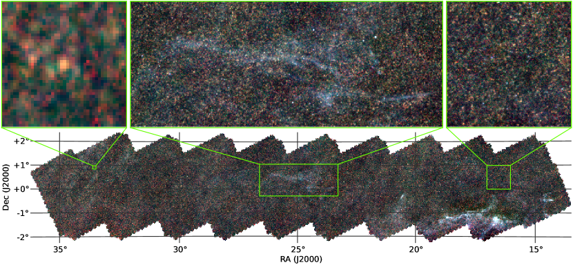
Figure 1.— Three-color image of the HerS field with 250, 350, and 500$\,\mathrm{\SIUnitSymbolMicro}$m as blue, green, and red, respectively. Note that 250 and 350$\,\mathrm{\SIUnitSymbolMicro}$m maps were convolved so that all three maps have the same angular resolution. Left Panel: A high-redshift candidate “red peaker”, with $S_{250}<S_{350}<S_{500}$, such that its SED suggests it lies somewhere between z of 3 and 7. Center Panel: A foreground cloud of Galactic cirrus (see § 5), with column densities reaching $N_{\rm H}\sim 4.5\times 10^{21}\,\rm cm^{-2}$. Right Panel: A typical $1^{\circ}\times 1^{\circ}$ “blank field”, which contains mostly dusty star-forming galaxies at intermediate to high redshifts.

The cosmic infrared background (CIB) traces the star-formation history of the Universe; roughly half the emission of young stars appears in the ultraviolet and optical, while the rest is absorbed by dust and then emitted at far-infrared wavelengths (Puget et al., 1996; Fixsen et al., 1998; Hauser & Dwek, 2001; Dole et al., 2006). Over the last decade a key goal of far-IR/submillimeter astronomy has been to identify the galaxies that produce the CIB. Recent deep surveys with the Balloon-borne Large Aperture Submillimeter Telescope (BLAST; Devlin et al., 2009; Marsden et al., 2009; Pascale et al., 2009) and the Herschel Space Observatory (H-ATLAS, HerMES, PEP; Eales et al., 2010; Oliver et al., 2012; Lutz et al., 2011) as well as ground-based submillimeter facilities such as LABOCA (LESS; Weiß et al., 2009) and SCUBA-2 (Geach et al., 2013) have “resolved” over 80% of the CIB at submillimeter wavelengths, via direct counting of sources (Oliver et al., 2010; Geach et al., 2013), P(D) techniques (Glenn et al., 2010), and stacking (Dole et al., 2006; Berta et al., 2011; Béthermin et al., 2012; Viero et al., 2013b). The resolution of this large fraction of the CIB into individual sources makes it clear that the CIB, at least near to its peak at $\sim 200$$\,\mathrm{\SIUnitSymbolMicro}$m, is dominated by a moderate luminosity population (i.e., $L_{\rm IR}\leq 10^{12}\,$L_⊙; Béthermin et al., 2011; Wang et al., 2013) in the broad redshift interval $1\leq z\leq 3$ (e.g., Viero et al., 2013a). Additionally, measurements of the CIB power spectrum (e.g., Amblard et al., 2011; Planck Collaboration et al., 2011c, 2013b; Viero et al., 2009, 2013b) yield estimates of the source clustering properties.

While the determination of these broad characteristics represents a remarkable achievement, much remains to be done to link the CIB, and the infrared (IR) luminous galaxies which make it up, to the general galaxy population. This goal requires determining the multi-wavelength characteristics of galaxies detected at far-IR/submillimeter wavelengths, and hence the physical properties that these wavelengths probe, e.g., rest-frame optical light tracing stellar mass, X-ray tracing black hole accretion, etc. A major complication is that the confusion-limited sensitivity of single-dish far-IR/submillimeter facilities is such that only the most luminous sources (i.e., $L_{\rm IR}\geq 10^{12}\,$L_⊙) can be individually detected in the key redshift range $1\leq z\leq 3$. Interferometric facilities like ALMA are not limited in this way, although their small fields of view (e.g. $\ll 1$ arcmin²) means that large blind surveys of the IR-galaxy population are inefficient and prohibitively expensive. To characterize the physical properties of the galaxies that dominate the CIB will instead require the use of statistical techniques, i.e., stacking or similar (Devlin et al., 2009; Marsden et al., 2009; Pascale et al., 2009; Kurczynski et al., 2012; Viero et al., 2012, 2013a; Roseboom et al., 2012), and hence very large numbers ($>100{,}000$) of galaxies detected at wavelengths with higher resolution (typically optical/near-IR).

Motivated by the importance of the CIB and the need to have large multi-wavelength surveys to understand its properties, we have conducted the Herschel Stripe 82 Survey (HerS; Figure 1). HerS consists of $79\,\rm deg^{2}$ of contiguous imaging with the SPIRE instrument (Griffin et al., 2010) on the Herschel Space Observatory (Pilbratt et al., 2010) to roughly the confusion limit ($\sim 7\,\rm mJy$ at the wavelengths 250, 350, and 500$\,\mathrm{\SIUnitSymbolMicro}$m; Nguyen et al., 2010). Crucially, HerS is positioned to overlap with a rich array of both existing and planned galaxy surveys in the Sloan Digital Sky Survey’s (SDSS; York et al., 2000) “Stripe 82” field, including: The SDSS-III’s Baryon Oscillation Spectroscopic Survey (BOSS; Eisenstein et al., 2011), VICS82 (VISTA+CFHT Stripe 82 survey; Geach et al. in prep.), VISTA-VIKING (Emerson et al., 2004), VLA-Stripe82 (Hodge et al., 2011), The Hobby-Eberly Telescope Dark Energy Experiment (HETDEX; Hill et al., 2008), The Spitzer-HETDEX Exploratory Large Area Survey (SHELA; Papovich et al., 2012), The Spitzer-IRAC Equatorial Survey (SpIES; Richards et al., 2012), and Hyper Suprime-Cam (HSC; Miyazaki et al., 2012) surveys. The combination of SHELA/SpIES, which are Spitzer-warm IRAC surveys of Stripe 82, and HETDEX, a wide-area spectroscopic survey targeting emission lines at $z>2$, will detect hundreds of thousands of galaxies and provide the key information required to interpret the HerS images.

In addition, HerS overlaps with a survey of the cosmic microwave background (CMB) conducted by The Atacama Cosmology Telescope (ACT; Sievers et al., 2013) in Stripe 82. The power in CMB maps on angular scales $\ell\,\lower 2.0pt\hbox{${>\atop\hbox{\raise 4.0pt\hbox{$\sim$}}}$}\,2000$ is dominated by point sources — both dusty and/or radio (e.g., Vieira et al., 2010; Das et al., 2011; Reichardt et al., 2012) — which act as foregrounds when attempting to study, for example, the damping tail of the CMB power spectrum (e.g., Keisler et al., 2011), or the thermal and kinetic Sunyaev Zel’dovich (SZ) effect from clusters or reionization, respectively (e.g., McQuinn et al., 2005). Cross-correlations between the CIB and CMB provide critical constraints for models of this contamination (e.g., Hajian et al., 2012; Planck Collaboration et al., 2013b), particularly on the smallest angular scales where the power spectrum is dominated by the non-linear, 1-halo term (e.g., Viero et al., 2013b). As we will later address, determining this component is one of the main motivations for locating the survey in the Stripe, and thus drives some of the mapmaking decisions.

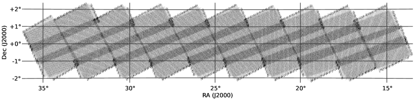
Figure 2.— Coverage map of the 350$\,\mathrm{\SIUnitSymbolMicro}$m data. The majority of the map is covered twice, while the dark grey stripes are the regions covered three times. As the scan orientations of the telescope at the ecliptic are fixed irrespective of the observing season, this scan strategy was chosen to guarantee complete coverage of the area along the Stripe.

In addition to these large statistical analyses, the large area of HerS adds an additional 79 deg² to the existing wide-area H-ATLAS and HerMES surveys to identify and study sources that are “rare” on the sky. The HerS field contains tens of nearby luminous IR galaxies (LIRGs; $L_{\rm IR}\geq 10^{11}\,$L_⊙) that are close enough to be resolved by Herschel at 250$\,\mathrm{\SIUnitSymbolMicro}$m. Meanwhile, we expect to identify close to 100 distant ($z>2$) galaxies with very high observed luminosities, with many of these resulting from lensing by foreground galaxies (like those found in e.g. Negrello et al., 2010; Wardlow et al., 2013; Vieira et al., 2013). Finally, HerS will contain many thousands of LIRGs at intermediate redshifts, making it a rich dataset for the study of IR-luminous galaxy evolution since $z=1$.

This paper describes the first release of HerS maps and catalog, including design strategy (§ 2), mapmaking and map properties (§ 3), and catalog construction and statistics (§ 4). Data are available at http://www.astro.caltech.edu/hers/.

2. Survey Design

HerS was designed to optimize cross-correlation measurements with ancillary data sets. This objective requires two key ingredients: well understood ancillary data (preferably of high source density); and submillimeter maps covering large areas with faithful reconstruction of large scales. To satisfy the first criterion, the survey was located in Stripe 82 which, in addition to the numerous surveys already described, will uniquely be observed by both HETDEX and ACT. Furthermore, its equatorial location — visible from most ground-based telescopes — makes it well-placed to be a valuable legacy field in the future. Its location was driven by the relatively low Galactic cirrus foreground (e.g., $N_{\rm H}\sim 1.7\times 10^{21}\,\rm cm^{-2}$; see § 3.5) with respect to the rest of the Stripe. Combined with the HeLMS survey (the largest field in HerMES; Oliver et al., 2012), the full $\sim 150\,\rm deg^{2}$ of Stripe 82 with $N_{\rm H}\leq 3\times 10^{21}\,\rm cm^{-2}$ has been imaged.

The second criterion — the need for large areas — is again due to source confusion. As shown in e.g., Acquaviva et al. (2008), the signal-to-noise ratio in cross-correlation measurements is proportional to the square root of $f_{\rm sky}$, or areal coverage, and is inversely proportional to the square root of the noise. For the case of maps observed with SPIRE, since the noise as a function of observing time quickly approaches the confusion limit, observation time is more optimally spent going wider rather than deeper. To reconstruct the largest scales, the maps were imaged in fast-scan mode ($60\,\rm arcsec\,s^{-1}$) and cross-linked with nearly orthogonal scans. The equatorial location of the field limited the orientations possible with the telescope. Coverage of the Stripe, visible in the coverage map shown in Figure 2, was achieved in 21 scans over 34.5 hours of observing time. This scan pattern resulted in 10 stripes with additional coverage, i.e., 3 rather than 2 scans; we address in later sections how these deeper stripes affect the noise properties of the maps and completeness properties of the catalogs.

3. Maps

Observations cover $79\,\rm deg^{2}$ in the equatorial Stripe 82, spanning $13^{\circ}$ to $37^{\circ}$ ($\rm 0^{h}54^{m}$ to $\rm 2^{h}24^{m}$) in RA, and $-2^{\circ}$ to $2^{\circ}$ in declination. Maps were made using the maximum likelihood mapmaker sanepic (Signal and Noise Estimation Procedure Including Correlations; Patanchon et al., 2008). This mapmaker is optimized for datasets where a large number of detectors observe the same area of the sky and the correlated (or common-mode) noise between the time-ordered data (TOD, or timestream) of these detectors cannot be ignored. The main source of this common-mode noise is the drift in temperature of the cooler bath surrounding the detector arrays. Instead of removing all large-scale variations with high-pass filtering, as many other mapmakers do, sanepic separates the low-frequency correlated noise from the sky signal, resulting in maps in which large-scale variations of the sky are better preserved.

Two sets of maps at 250, 350, and 500$\,\mathrm{\SIUnitSymbolMicro}$m were made in order to accommodate different science goals. For the first set, we used a tangent plane (TAN) projection with pixel sizes of 6, 8.33 and 12 arcsec for the 250, 350, and 500$\,\mathrm{\SIUnitSymbolMicro}$m maps, respectively. These values are typical for SPIRE maps, chosen to correspond to roughly one-third of the size of the SPIRE beams (18.1, 25.2 and 36.6 arcsec full-width at half-maximum). Since the HerS field overlaps with the equatorial Stripe observed by the Atacama Cosmology Telescope (ACT), we also made maps using the nominal ACT map projection for cross-analysis of the two data sets. The motivation for matching pixels is that it avoids the reprojecting/regridding of maps that would be necessary to perform map-based operations — whether in Fourier space or otherwise — which could potentially introduce systematic uncertainties. The HerS-ACT maps were made using a cylindrical equal-area (CEA) projection with pixel sizes of 29.7 arcsec in all three bands, corresponding to the nominal ACT pixel size.

3.1. Data preprocessing

The raw data from the bolometer arrays are stored as separate TODs for each detector. Before the data are fed into our mapmaker several preprocessing steps are applied to the raw TODs. We used the HIPE (Herschel Interactive Processing Environment; Ott, 2010), version 11.0.1 mapmaking software package to convert the uncalibrated raw TODs into the so-called Level 1 format, which is the input format used by mapmakers. The preprocessing steps involve detecting jumps in the signal, flagging glitches, and correcting for the low-pass filter response of the electronics and for the bolometer time response. Calibration of the data also happens at this early processing stage. The Level 1 data are read in by the smap mapmaking software package (Levenson et al., 2010; Viero et al., 2013b) and exported to the format accepted by sanepic. smap also uses an additional iterative glitch detection algorithm during mapmaking, and the deglitching information can be re-used later. This existing deglitching-information from preliminary HerS maps created with smap is also applied to our TODs. For details of these preprocessing steps see appendix A of Viero et al. (2013b). Both the HIPE and smap pipelines have their own algorithms to remove temperature drifts on long timescales by fitting to thermistor TODs. Since sanepic is optimized to deal with large-scale correlated noise, we turn off the temperature drift removal step in HIPE and smap during preprocessing. The last preprocessing steps are applied by sanepic. A first-order polynomial is fit to and removed from each data segment, because the variations on timescales longer than the timestream itself can cause leakage during Fourier-transformation, which would introduce artifacts in our maps. sanepic fills any gaps in the TODs and the data segments are apodized at the edges over 50 samples. This measure is needed since the mapmaker assumes that the ends of each data segment are strongly correlated (“circular”).

3.2. Mapmaking

The sanepic mapmaking method is described in detail in Patanchon et al. (2008); here we review the salient points. The timestream of a bolometer indexed by i can be modeled as

$$d_{i}(t)=\sum\limits_{p}A_{ip}(t)s_{p}+n_{i}(t),$$ (1)

where t is the time when the sample was taken, $s_{p}$ is the signal in pixel p of the map of the sky and $A_{ip}(t)$ is the pointing matrix, which gives the weight of the contribution of the signal in pixel p to the timestream of bolometer i at time t. We assert that $s_{p}$ corresponds to the beam-convolved sky, in which case the pointing matrix tells us the position where bolometer i points on the sky at time t. The noise term $n_{i}(t)$, whose properties are assumed to be stationary, is the sum of two components: the uncorrelated noise between different detectors $\tilde{n}_{i}(t)$; and a common-mode signal, $\alpha_{i}c(t)$, seen by all detectors at a given time. This “noise” term is

$$n_{i}(t)=\tilde{n}_{i}(t)+\alpha_{i}c(t),$$ (2)

where c(t) is the correlated noise which is the same for all detectors apart from a detector-dependent multiplicative factor $\alpha_{i}$. The sky signal can be estimated from the detector TODs using maximum likelihood methods. The solution is given by

$$\hat{s}=(A^{\rm T}N^{-1}A)^{-1}A^{\rm T}N^{-1}d,$$ (3)

where $N^{-1}$ represents the inverse of the time-domain noise covariance matrix. This can be calculated as

$$N^{-1}=\mathcal{F}^{-1}[P(\omega)^{-1}],$$ (4)

where $\mathcal{F}$^-1 represents the inverse Fourier-transformation and $P(\omega)$ is a matrix constructed from the auto- and cross-power spectra of the TODs, containing information about the detectors common-mode noise, in addition to the uncorrelated noise terms:

$$P^{-1}(\omega)=[\alpha\langle c(\omega)^{\dagger}c(\omega)\rangle\alpha^{t}+\langle\tilde{n}^{\dagger}(\omega)\tilde{n}(\omega)\rangle]^{-1}.$$ (5)

The inverse of the pixel-pixel noise covariance matrix, $N^{-1}_{pp^{\prime}}=(A^{T}N^{-1}A)^{-1}$ is not calculated explicitly. The mapmaker uses an iterative algorithm based on the conjugate gradient method with preconditioner to find the maximum likelihood solution for the map. Usually a few hundred iterations are needed to reach convergence. The computational time scales with the square of the number of bolometers and also depends on the number of samples, $n_{s}$, in the TOD as $n_{s}{\rm log}(n_{s})$. Our observations consist of 34.5 hours of data for each bolometer sampled at a frequency of 18.6 Hz. The 250$\,\mathrm{\SIUnitSymbolMicro}$m array has the largest number of bolometers (139) so the map created from this data has the longest processing time. Using eight 2.8 GHz processors (Intel Xeon X5560 CPUs) the mapmaker needs about 17 hours to reach convergence at 250$\,\mathrm{\SIUnitSymbolMicro}$m.

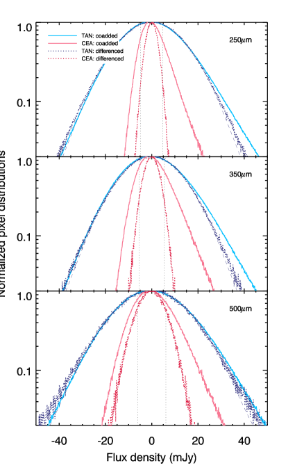
Figure 3.— Pixel flux distributions of the coadded (i.e., the sky) and differenced jackknife maps, represented as solid and dotted lines, respectively, for both TAN (wider light/dark blue) and CEA (narrower red/pink) projections. Coadded maps include the entire data set in each band, while in the differenced maps the sky signal has been removed, leaving only instrumental noise. Coadded histograms are thus wider because they include confusion noise, represented by vertical dashed lines from Nguyen et al. (2010), as well as an excess compared with a Gaussian at brighter flux densities from resolved sources. The full width at half maxima of the best-fit Gaussian to the difference maps — shown as faint blue and red dashed lines for TAN and CEA , respectively — represent average instrumental noise levels. Note that the TAN maps with their smaller pixels are dominated by instrumental noise, while the bigger pixel CEA maps have approximately equal contributions from instrument and confusion noise.

3.3. Noise properties

To examine the properties of the residual noise in our signal maps, we create “jackknife” difference maps, i.e., the timestream data are split into two halves and a separate map is made for each half, and the difference map is then made by multiplying one of the jackknifes by minus one and then averaging the two together. This process removes the astronomical signal but retains the noise, as the jackknife difference map contains the same instrumental noise properties as the coadded sky map. There are in principle several different ways to split the data in half, some more effective than others, but the shallow depth of the HerS observations in practice limits our options. For example, since the field is only scanned once in each orthogonal direction, we cannot split the TODs into two halves based on observation time, and splitting the datasets by orthogonal scan-direction results in maps that have strong residual correlated noise along the scan directions, due to lack of cross-linking. A third way to split the data is to divide up the detector focal planes, and only use every second bolometer to make our maps. Even though this method gives the best coverage, at the nominal pixel sizes the resulting maps are still quite sparse, especially at 500$\,\mathrm{\SIUnitSymbolMicro}$m where the sampling density is the lowest. This problem is not present in the larger pixel-size maps corresponding to the ACT mapping, and after correcting for the effect of the bigger pixel size we recover values similar to those in the more finely sampled maps.

In Figure 3 we plot pixel-histograms of the coadded (or sky) and differenced jackknife maps — in shades of blue for the standard (TAN) maps and red for the HerS-ACT (CEA) maps — as solid and dotted lines, respectively. The coadded jackknife maps contain both instrument and confusion noise (the latter illustrated as vertical dotted lines), and are thus wider than the differenced jackknife maps. However, while the instrument noise is the dominant contribution in the TAN maps, the instrument noise in the HerS-ACT CEA maps is lower, by virtue of their pixels being 24.5, 12.7, $6.1\times$ larger (by area) at 250, 350, and 500$\,\mathrm{\SIUnitSymbolMicro}$m, respectively, such that they have approximately equal contributions from instrument and confusion noise.

Instrumental noise levels are calculated by fitting a Gaussian to the pixel-histogram of the differenced jackknife maps for both the TAN and CEA cases. We find that the noise is extremely well described by the Gaussian fit (shown as thin dashed lines in the Figure 3), deviating only at 500$\,\mathrm{\SIUnitSymbolMicro}$m by less than 2%, and that the deviation is explained by the non-uniformity in the samples per pixel arising from the sparseness of the array and the fact that we only cover each area with two scans. The resulting $1\sigma$ values in the TAN (CEA) maps are 11.9 (2.2), 11.4 (3.1), and 13.5 (5.4) $\rm mJy\,beam^{-1}$ at 250, 350, and 500$\,\mathrm{\SIUnitSymbolMicro}$m, respectively. Note that since the coverage of the HerS maps is not completely uniform (seen clearly in Figure 2), the noise levels where more than two orthogonal scans overlap is lower. In the deeper regions of the TAN (CEA) maps, the noise levels are 10.7 (2.1), 10.3 (2.8), and 12.3 (4.9) $\rm mJy\,beam^{-1}$, while in the shallower regions they are 13.3 (2.5), 12.7 (3.4), and 14.9 (6.0) $\rm mJy\,beam^{-1}$ at 250, 350, and 500$\,\mathrm{\SIUnitSymbolMicro}$m, respectively.

sanepic also creates an error map as an extension to the output products. This map gives an estimate of the variance of the noise in each pixel of the final map. Obtaining this error term correctly would require calculating the explicit pixel-pixel noise covariance matrix, but that operation is too computationally intensive and is never carried out during the iterative mapmaking. The error map sanepic creates is a first-order estimate of this noise, computed by neglecting the off-diagonal terms in the inverse pixel-pixel noise covariance matrix, assuming that the final map only contains white noise. These determinations over-estimate the real residual noise values in the maps, but the error map can still be used to assign weights to each pixel in our final map.

Figure 4.— Transfer function, $T$, of the sanepic mapmaker at 500$\,\mathrm{\SIUnitSymbolMicro}$m, estimated with a Monte Carlo simulation as described in § 3.4. $T$ is found to be approximately unity down to $\ell\sim 200$ ($\sim 1\,\rm deg$), dropping to 0.5 at $\ell\sim 30$. The vertical dashed line represents the largest accessible scale, given the finite size of the survey, showing that effectively all scales in the map are reconstructed. Upper axis indicates $k_{\theta}\equiv\ell/(2\pi)$.

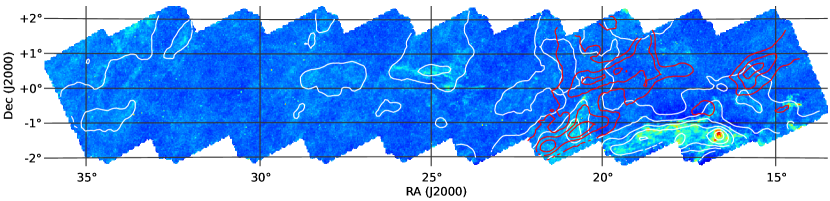
Figure 5.— HerS 250$\,\mathrm{\SIUnitSymbolMicro}$m map, smoothed to 2 arcmin, overlaid with contours representing the column density of local velocity clouds (white) and IVCs (red), as traced by H i  emission from GASS 21-cm data. Note that no HVCs appear in this field. White contours show $N_{\rm H}$ at 3.4, 4.2, 5.0, 5.8, 6.6, and $7.4\times 10^{21}\,\rm H\,cm^{-2}$, while red contours show $N_{\rm H}$ at 0.5, 0.8, and $1.1\times 10^{21}\,\rm H\,cm^{-2}$. The color scale ranges linearly from -25 (blue) to 80 mJy (red). The vast majority of the cirrus visible in HerS is attributable to the local velocity component.

3.4. Transfer Function

We investigate how reliable our mapmaker is in reconstructing large-scale structure on different angular scales. This assessment is made by creating simulated pure-signal maps, which are then reprojected into detector TODs and fed back into our mapmaker the same way as for the real data. The ratio of the azimuthally-averaged Fourier transform of the reconstructed map and the pure-signal input map gives us the mapmaker’s transfer function. In the ideal case the ratio should be unity at all spatial scales. However, the mapmaker can introduce false signal to our maps, or remove existing power, which would appear as a deviation from unity in the transfer function. On the scales where the deviation from unity is not too large, we can correct for these effects. We created 100 pure signal maps with a power-law power spectrum resembling that of the cosmic infrared background without the cirrus, and “observed” them with a Monte Carlo simulation at 500$\,\mathrm{\SIUnitSymbolMicro}$m, though we check that the transfer function is the same at all wavelengths with a small subset of simulated maps. Figure 4 shows the resulting transfer function. The mapmaker can successfully reconstruct all large scales that are accessible in our maps. The simulated and reconstructed maps were made with the same pixel size, so the pixel window function does not have any effect here, and the transfer function remains unity on small scales. The transfer function only starts to drop for $\ell\,\lower 2.0pt\hbox{${<\atop\hbox{\raise 4.0pt\hbox{$\sim$}}}$}\,200$, corresponding to approximately half of the narrowest extent of our survey.

3.5. Galactic Cirrus

Thermal emission by diffuse interstellar dust in our Galaxy — the diffuse Galactic cirrus — can be described by a modified blackbody proportional to $\nu^{\beta}B(\nu)$, where $B(\nu)$ is the Planck function and $\beta$ is the emissivity index, with temperatures ranging from 17 to 20 K in the most diffuse regions (e.g., Boulanger et al., 1996; Bracco et al., 2011), to as low as 14 K in dense regions where molecular hydrogen (H₂) can form (e.g., Netterfield et al., 2009; Planck Collaboration et al., 2011b), peaking in emission between 150 and 200$\,\mathrm{\SIUnitSymbolMicro}$m.

In diffuse regions, dust is well-traced by atomic hydrogen gas (H i) which emits at 21 cm and in the radio (e.g., Boulanger et al., 1996). H i data are available for HerS from the Parkes Galactic All-Sky Survey (GASS; McClure-Griffiths et al., 2009; Kalberla et al., 2010), a 1.4 GHz survey of Galactic atomic hydrogen emission, taken with the Parkes 64-m radio telescope, over $>20{,}000\,\rm deg^{2}$. Publicly available data are provided as velocity cubes, with effective angular resolution of $16\mathrm{\SIUnitSymbolArcminute}$, and velocity resolution of $1.0\,\rm km\,s^{-1}$. Following Planck Collaboration et al. (e.g., 2011a), we divide the cubes by velocity with respect to the local frame of reference into local ($|v_{\rm LSR}|<30\,{\rm km\,s^{-1}}$) and intermediate velocity clouds (IVCs; $|v_{\rm LSR}|>30\,{\rm km\,s^{-1}}$). Note that no HVCs are visible in this field. We plot contours of the local and IVC components in Figure 5 (white and red contours, respectively), showing that the cirrus emission in HerS comes predominantly from the local velocity component.

For column densities of roughly $N_{\rm H}\,\lower 2.0pt\hbox{${<\atop\hbox{\raise 4.0pt\hbox{$\sim$}}}$}\,4\times 10^{21}\,\rm cm^{-2}$, and on scales of an arcminute or less, this foreground is easily suppressed with a high-pass or matched filter (e.g., Chapin et al., 2011). High concentrations of H i (and potentially H₂) — such as that present in the bottom right corner of the HerS maps — present a greater challenge; we describe our filtering method for point source identification in § 4.

4. Catalog

We now present the first HerS band-merged catalog. We caution the user that because of the uneven coverage of the survey, the density of high signal-to-noise sources is higher in the deep stripes. Thus, though the catalog is suitable for applications such as cross-identification of bright objects, or cross-correlations given appropriate weights, etc., it should not be used for estimating statistically rigorous quantities such as source counts. That does not mean that they cannot be measured, just that such operations are better done using the maps themselves, where the detailed properties of the extraction technique vs. survey depth, etc., and the resulting catalog, can be properly simulated.

4.1. Catalogue production

Point-source catalogs across the HerS field in the three SPIRE bands were produced using a three-step process: map filtering (to remove large-scale Galactic cirrus); source identification; and source extraction or photometry. We now describe the details of each of these steps in turn.

Filtering of the HerS maps is done using a tapered high-pass filter that begins to remove power on scales larger than three times the beam FWHM at each SPIRE band. Specifically, we take the 2D Fourier transform of each map and attenuate spatial frequencies lower than $k=1/b,{\rm arcmin}^{-1}$ by a factor $(kb)^{3}$, where $b=3\times\mathrm{FWHM}$ in arcmin i.e.,

$$d_{\mathrm{f}}(x,y)=\begin{cases}\mathcal{F}^{-1}k\geq 1/b,&\hat{f}(l,m)\\ \mathcal{F}^{-1}k<1/b,&{\hat{f}(l,m)}{(kb)^{3}}\\ \end{cases},$$ (6)

where $d_{\mathrm{f}}$ is the filtered map, $\hat{f}(l,m)$ is the Fourier transform of the observed map with frequencies $l$ and $m$ in the x and y directions, respectively, and $k=\sqrt{l^{2}+m^{2}}$.

The minimum filtering scale of $(3\times\mathrm{FWHM})^{-1}$ was chosen to preserve as much of the source profile as possible while still suppressing any non-point like structure in the map. In Figure 7 we illustrate the effectiveness of this filtering on a $36\mathrm{\SIUnitSymbolArcminute}\times 36\mathrm{\SIUnitSymbolArcminute}$ region of the HerS 250$\,\mathrm{\SIUnitSymbolMicro}$m image that is badly affected by cirrus contamination, with all power on scales larger than the beam efficiently suppressed. Consequently, negative “bowls” are visible around the brightest sources; next we describe how this is addressed when extracting point sources by filtering the point-spread function (PSF).

Identification of point sources in the filtered 250$\,\mathrm{\SIUnitSymbolMicro}$m image using the IDL software package starfinder (Diolaiti et al., 2000). Sources are assumed to be exclusively point-like in the SPIRE images, with a PSF described by a circular 2D Gaussian with FWHM of 18.15, 25.15 and 36.3 arcsec for 250, 350, and 500$\,\mathrm{\SIUnitSymbolMicro}$m, respectively. To account for the effect of our Fourier filtering (i.e., the “bowls”) the PSF is filtered in the same way as the map and this filtered PSF is used in the subsequent source detection and extraction steps. While starfinder can operate in an “iterative” mode, detecting and removing sources at decreasing signal-to-noise ratio (SNR) thresholds, so as to allow the identification of faint sources in crowded regions, here we use a single pass of starfinder requiring peak $\rm SNR>3$ and $\rho_{\rm PSF}$, the correlation coefficient, to be greater than 0.5. In this setup starfinder can be considered to be a simple peak finder; pixels in the map with $\rm SNR>3$ are identified, collated into independent peaks, and then cross-correlated with the known PSF to confirm they are truly sources and not simply noise. Note that the uneven coverage of the maps, and subsequent deeper stripes (Figure 2) with lower noise properties (3.3), leads to a higher density of $\rm SNR>3$ sources in the deep regions.

Source photometry is performed using a modified version of the De-blended SPIRE Photometry (desphot) algorithm (Roseboom et al., 2010, 2012, henceforth R12; Wang et al., in prep.) developed for use on SPIRE data from the HerMES project (Oliver et al., 2012). The main advantage of this approach is that it deals with the source blending issue in a way more appropriate to SPIRE maps than starfinder, and produces consistent, band-merged SPIRE catalogues by using the input sources at the highest resolution band (250$\,\mathrm{\SIUnitSymbolMicro}$m) as a prior for the other SPIRE wavelengths.

While a complete description of how desphot works is given in the above-listed papers, we briefly summarize the main points here. For source photometry, desphot assumes that the map (or each map segment) can be described as the summation of the flux density from the $n$ known sources in the map, i.e.,

$${\bf d}=\sum_{i=1}^{n}{\bf P}f_{i}+\delta,$$ (7)

where d is the image data, P the PSF for source $i$, ${f_{i}}$ the flux density of source $i$, and $\delta$ an unknown noise term. As discussed in Roseboom et al. (2010) a linear equation of this form will (as in § 3.2) have a maximum likelihood solution

$${\bf\hat{f}}=({\bf A}^{\rm T}{\bf N_{d}}^{-1}{\bf A})^{-1}\,{\bf A}^{\rm T}{\bf N_{d}}^{-1}{\bf d},$$ (8)

where A is an $m$ pixel by $n$ source matrix that describes the PSF for each source in the map and ${\bf N_{d}}$ is the noise covariance matrix. The best non-negative solution for ${\bf\hat{f}}$ is found using the lasso algorithm, as described in R12. As it is not computationally feasible to solve for the full set of $\sim 30{,}000$ sources simultaneously, the input list must be broken up into “groups” of sources that have significant overlap. In R12 this is accomplished by identifying high SNR “islands” in the SPIRE maps, but the HerS images are simply too big for this to be a reasonable option. Thus we group the desphot input list with a “friends-of-friends algorithm”, specifically the spheregroup routine available as part of the SDSS idlutils, using a linking length of 3 arcmin. Friends-of-friends clustering algorithms have been used extensively in astronomy, typically for the identification of halos in dark matter simulations (e.g., Davis et al., 1985). The algorithm works simply to uniquely group sources which are separated by less than the linking length. Groups are collated by identifying common neighbors (“friends”) so that each source belongs uniquely to one group.

Despite the relatively shallow nature of the HerS observations, confusion is still a significant contributor to the noise budget for point sources. This complicates the selection criteria for a useful source catalogue as the point source detection stage described above isolates sources with a $\rm SNR>3$, taking into account only the instrumental noise. For example, at 250$\,\mathrm{\SIUnitSymbolMicro}$m point sources in the shallow (deep) region have a mean instrumental noise, estimated via error propagation of the hits map, of 7.7 (6.3) mJy, while the total noise, estimated via the pixel distribution of the point-source convolved map, is 11.1 (10.2) mJy. Note that these noise figures differ from those presented in Section 3.3, as here we are considering the noise not in a single map pixel, but integrated over a point source. To proceed we follow a similar approach as Smith et al. (2012): the confusion noise is assumed to be constant across the entire map and is estimated via $\sigma_{\mathrm{conf.}}^{2}=\sigma_{\mathrm{total}}^{2}-\langle\sigma_{\mathrm{inst.}}\rangle^{2}$, where $\sigma_{\mathrm{total}}^{2}$ is the variance of the point source convolved map, and $\langle\sigma_{\mathrm{inst.}}\rangle$ is the mean instrumental noise in the map. The total noise for each source $i$ is then taken to be $\sigma_{i}^{2}=\sigma_{\mathrm{conf.}}^{2}+\sigma_{\mathrm{inst.},i}^{2}$. Using this approach we get $\sigma_{\mathrm{conf.}}=8$ mJy for each of the 250, 350, and 500$\,\mathrm{\SIUnitSymbolMicro}$m band. These values are slightly higher than those presented by Nguyen et al. (2010) and Smith et al. (2012); this is likely due to the effect of the Fourier filtering. Using this definition of the the total noise, $\sigma$, for sources in our catalogue we threshold the catalogue to only include sources with $S_{250}>3\sigma$. For sources in the shallow regions this limit translates to $S_{250}\geq 31$ mJy while for the deep regions it is $S_{250}\geq 28$ mJy

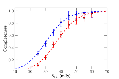
Figure 6.— HerS Catalog Completeness at 250$\,\mathrm{\SIUnitSymbolMicro}$m estimated by injecting grids of mock sources into the map. The blue points show the completeness in the deep region, while the red points are the shallow regions. The dashed lines are logistic fits to the data; $C=1/(1+\exp(0.145S_{250}+\beta))$, where $\beta=4.4$ for the deep regions, and $\beta=5.4$ for the shallow region.

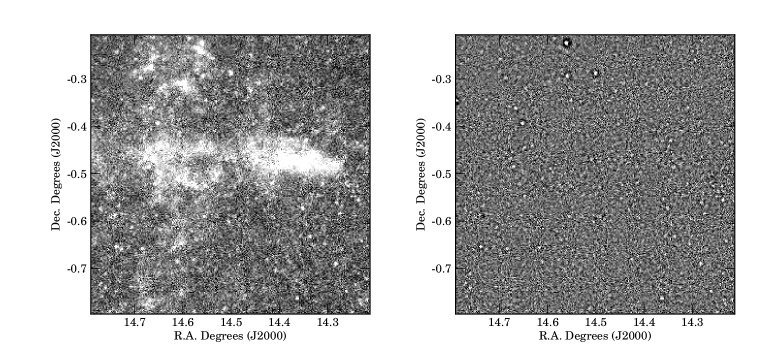
Figure 7.— $36\mathrm{\SIUnitSymbolArcminute}\times 36\mathrm{\SIUnitSymbolArcminute}$ cutout from the HerS 250$\,\mathrm{\SIUnitSymbolMicro}$m map, in a region badly affected by Galactic cirrus. The cutout on the left is with no filtering, while the one on the right is with the tapered Fourier filtering described in the text. The effectiveness of the filter in removing large-scale features can be seen, but it also makes negative “bowls” around the brightest features, which must be accounted for by filtering the PSF when extracting sources.

4.2. Completeness and Reliability

The completeness and reliability of the HerS catalogue is assessed using Monte Carlo techniques. The completeness is estimated by injecting grids of sources into the HerS maps and measuring the fraction that are detected (as $3\sigma$ sources) using the photometry pipeline. The input grids are matched to the output catalogue using a 6 arcsec matching radius, which we estimate will produce spurious matches between unassociated input mock sources and real SPIRE sources at a rate of 0.5%. As the HerS catalogue makes use of a 250$\,\mathrm{\SIUnitSymbolMicro}$m prior (i.e., we do not consider sources undetected at 250$\,\mathrm{\SIUnitSymbolMicro}$m) only the completeness at this wavelength is assessed. Figure 6 presents the completeness as a function of 250$\,\mathrm{\SIUnitSymbolMicro}$m flux density for the HerS catalogue in both the deep and shallow regions. It is reasonable to expect that the completeness, $C$, follows a logistic function, i.e., $C=1/(1+\exp\{\alpha S+\beta\})$. For both the deep and shallow completeness data we fit for the parameters $\alpha$ and $\beta$, finding $\alpha=0.145$ for both regions, while $\beta=4.4$ for the deep region and $\beta=5.4$ for the shallow region.

It is worth noting that this assessment of the completeness only considers the recoverability of sources at a given true flux density; at low SNR, the measured flux densities will be strongly affected by Eddington-type bias, i.e., $\langle S_{\rm obs}\rangle>\langle S_{\rm true}\rangle$. While the true impact of such flux boosting can only be assessed by taking into account the true distribution of flux densities (i.e., the number counts; Coppin et al., 2006), from our analysis we determine that $S_{250}\sim 40\,$mJy is the faintest tested flux density at which the mean recovered flux density is equal to the injected value, i.e., $\langle S_{\rm obs}\rangle=\langle S_{\rm true}\rangle$.

The reliability is estimated by taking jackknife realizations of the noise from deeper SPIRE imaging in the CDFS-SWIRE field. The HerMES observations of the CDFS-SWIRE field consist of eight scans of an 8 deg² region with SPIRE in fast scan mode. Thus we can produce four jackknife noise realizations at the depth of the HerS observations (2 scans) by producing maps from different pairs of scans in CDFS and subtracting away the eight scan maps. In order to assess the reliability of the HerS catalogue we run the pipeline on these noise-only maps. Across the four noise realizations (32 deg²) we detect 39 spurious sources at 3$\sigma$, giving a false positive rate of $1.2\pm 0.2$ deg^-2. Thus across the 79 deg² of HerS we expect $96\pm 16$ spurious sources.

4.3. Details of the Published Catalog

Beginning with the catalog output by desphot, we implement the following quality cuts: First we apply a 3$\sigma$ cut, where the completeness is estimated to be 50% (from Figure 6) and false detection rate to be less than 1%, as well as require reasonable residuals (i.e., $\chi^{2}<10$). Next, we identify obviously extended sources — 24 in total — where their extended nature results in them being broken up into multiple components by the filter, and remove them. This results in a catalogue with 32,815 sources at 250$\,\mathrm{\SIUnitSymbolMicro}$m, of which 13,300 and 3,276 have similarly defined 3$\sigma$ detections at 350 and 500$\,\mathrm{\SIUnitSymbolMicro}$m, respectively.

Sources fall in three distinct regions, identified with flag in the catalog as either 0) in the deep regions (16,626 sources); 1) in the wide regions (14,083 sources); or 3) on the edges (2,106 sources). Wide regions are defined as those having the nominal coverage of two scans, while deep regions are those with three (and sometimes, but rarely, four) scans. Edges are the areas with only one scan of coverage. Local counterparts of the extended sources are listed by name in the README posted in the same directory.

5. Conclusion

We present and make publicly available the first set of maps at 250, 350, and 500$\,\mathrm{\SIUnitSymbolMicro}$m, and catalog with $3.3\times 10^{4}$ sources detected at a significance of $\,\lower 2.0pt\hbox{${>\atop\hbox{\raise 4.0pt\hbox{$\sim$}}}$}\,3\sigma$ (including confusion noise), from the Herschel Stripe 82 Survey. Maps are made with the optimal mapmaker sanepic, which we demonstrate recovers emission on all scales that are in principle accessible. The survey encompasses approximately half of the $150\,\rm deg^{2}$ of the deep SDSS Stripe in which Galactic foregrounds are subdominant at submillimeter wavelengths (with HeLMS, described in Oliver et al., 2012, covering the other half). Approximately $\sim 10\%$ of the HerS maps have significant foreground, with column densities $N_{\rm H}\,\lower 2.0pt\hbox{${>\atop\hbox{\raise 4.0pt\hbox{$\sim$}}}$}\,4\times 10^{21}\,\rm cm^{-2}$ and have been shown to be composed predominantly of local velocity clouds.

The band-merged catalog is constructed, after filtering, with desphot (Roseboom et al., 2010), using 250$\,\mathrm{\SIUnitSymbolMicro}$m sources (extracted with starfinder) as positional priors. We include sources with signal-to-noise greater than 3, whose completeness is estimated to be 50% (Figure 6), and false detection rate less than 1%.

HerS was designed with the intention of cross-correlating the maps with ancillary data — whether maps or catalogs of galaxies or clusters — to address a wide variety of questions. It was initially proposed to correlate with HETDEX Lyman $\alpha$ emitters (LAEs) at $1.8<z<3.5$ (e.g., Hill et al., 2008; Adams et al., 2011) with the aim of measuring the contribution to the CIB from that redshift range and infer the star-formation rate density through this critical epoch. Furthermore, combining that measurement with stellar masses of LAEs estimated from the SHELA/SpIES catalogs, specific star-formation rates, and the relationship of star-formation to halo mass at higher-$z$ can be explored.

Other exciting projects that we intend to pursue include: determining the correlation between HerS sources and clusters or cluster members, e.g., exploring the correlation of infrared emitting sources and clusters detected by ACT using the SZ effect (Hasselfield et al., 2013); the lensing of the CMB by foreground structure traced by the CIB (Holder et al., 2013; Planck Collaboration et al., 2013a; Hanson et al., 2013), and investigating the effect that the environment has on star-formation in sources identified as cluster members (Geach et al., 2012; Rykoff et al., 2013). SDSS/BOSS offers a wealth of galaxy and quasar (e.g., Ross et al., 2009; Pâris et al., 2012) populations for cross-correlation.

In addition to cross-correlations, single-object lensed or highly luminous high-redshift sources can be selected from the maps themselves. By linearly combining the maps, high-redshift “red peakers” (e.g., with $S_{250}<S_{350}<S_{500}$ at $z\,\lower 2.0pt\hbox{${>\atop\hbox{\raise 4.0pt\hbox{$\sim$}}}$}\,3$; Dowell et al., 2014; Riechers et al., 2013) are identifiable. High-redshift groups and clusters can be selected as red overdensities (e.g., the Planck clumps; Clements et al., submitted), which alternatively can be used to clean the CIB from CMB maps to probe the damping tail of the CMB power spectrum (e.g., Hajian et al., 2012; Keisler et al., 2011; Reichardt et al., 2012; Sievers et al., 2013).

Studies focused on our Galaxy are possible as well. The large-scale fidelity of our maps, as demonstrated by the transfer function shown in Figure 4, allows large-scale properties of cirrus and dense molecular regions to be fully reconstructed, while our relatively small beam means that finer structures can be separated out. And by correlating dust emission in the infrared with measurements from optical fibers pointed at “blank sky”, we can recover the optical spectrum of the diffuse Galactic light to constrain the size distribution of Galactic dust (e.g. Brandt & Draine, 2012).

Finally, future cosmological surveys such as the Dark Energy Survey (DES), Hyper Suprime-Cam (HSC), and the Large Synoptic Survey Telescope (LSST) will further enrich the density and variety of sources with which these submillimeter data can be cross-correlated, making this survey an integral component of an important Legacy field.

References

- Acquaviva et al. (2008) Acquaviva, V., Hajian, A., Spergel, D. N., & Das, S. 2008, Phys. Rev. D, 78, 043514
- Adams et al. (2011) Adams, J. J., Blanc, G. A., Hill, G. J., Gebhardt, K., Drory, N., Hao, L., Bender, R., Byun, J., et al. 2011, ApJS, 192, 5
- Amblard et al. (2011) Amblard, A., Cooray, A., Serra, P., Altieri, B., Arumugam, V., Aussel, H., Blain, A., Bock, J., et al. 2011, Nature, 470, 510
- Berta et al. (2011) Berta, S., Magnelli, B., Nordon, R., Lutz, D., Wuyts, S., Altieri, B., Andreani, P., Aussel, H., et al. 2011, A&A, 532, A49
- Béthermin et al. (2011) Béthermin, M., Dole, H., Lagache, G., Le Borgne, D., & Penin, A. 2011, A&A, 529, A4
- Béthermin et al. (2012) Béthermin, M., Le Floc’h, E., Ilbert, O., Conley, A., Lagache, G., Amblard, A., Arumugam, V., Aussel, H., et al. 2012, A&A, 542, A58
- Boulanger et al. (1996) Boulanger, F., Abergel, A., Bernard, J.-P., Burton, W. B., Desert, F.-X., Hartmann, D., Lagache, G., & Puget, J.-L. 1996, A&A, 312, 256
- Bracco et al. (2011) Bracco, A., Cooray, A., Veneziani, M., Amblard, A., Serra, P., Wardlow, J., Thompson, M. A., White, G., et al. 2011, MNRAS, 412, 1151
- Brandt & Draine (2012) Brandt, T. D. & Draine, B. T. 2012, ApJ, 744, 129
- Chapin et al. (2011) Chapin, E. L., Chapman, S. C., Coppin, K. E., Devlin, M. J., Dunlop, J. S., Greve, T. R., Halpern, M., Hasselfield, M. F., et al. 2011, MNRAS, 411, 505
- Coppin et al. (2006) Coppin, K., Chapin, E. L., Mortier, A. M. J., Scott, S. E., Borys, C., Dunlop, J. S., Halpern, M., Hughes, D. H., et al. 2006, MNRAS, 372, 1621
- Das et al. (2011) Das, S., Marriage, T. A., Ade, P. A. R., Aguirre, P., Amiri, M., Appel, J. W., Barrientos, L. F., Battistelli, E. S., et al. 2011, ApJ, 729, 62
- Davis et al. (1985) Davis, M., Efstathiou, G., Frenk, C. S., & White, S. D. M. 1985, ApJ, 292, 371
- Devlin et al. (2009) Devlin, M. J., Ade, P. A. R., Aretxaga, I., Bock, J. J., Chapin, E. L., Griffin, M., Gundersen, J. O., Halpern, M., et al. 2009, Nature, 458, 737
- Diolaiti et al. (2000) Diolaiti, E., Bendinelli, O., Bonaccini, D., Close, L., Currie, D., & Parmeggiani, G. 2000, A&AS, 147, 335
- Dole et al. (2006) Dole, H., Lagache, G., Puget, J.-L., Caputi, K. I., Fernández-Conde, N., Le Floc’h, E., Papovich, C., Pérez-González, P. G., et al. 2006, A&A, 451, 417
- Dowell et al. (2014) Dowell, C. D., Conley, A., Glenn, J., Arumugam, V., Asboth, V., Aussel, H., Bertoldi, F., Béthermin, M., et al. 2014, ApJ, 780, 75
- Eales et al. (2010) Eales, S., Dunne, L., Clements, D., Cooray, A., de Zotti, G., Dye, S., Ivison, R., Jarvis, M., et al. 2010, PASP, 122, 499
- Eisenstein et al. (2011) Eisenstein, D. J., Weinberg, D. H., Agol, E., Aihara, H., Allende Prieto, C., Anderson, S. F., Arns, J. A., Aubourg, É., et al. 2011, AJ, 142, 72
- Emerson et al. (2004) Emerson, J. P., Sutherland, W. J., McPherson, A. M., Craig, S. C., Dalton, G. B., & Ward, A. K. 2004, The Messenger, 117, 27
- Fixsen et al. (1998) Fixsen, D. J., Dwek, E., Mather, J. C., Bennett, C. L., & Shafer, R. A. 1998, ApJ, 508, 123
- Geach et al. (2012) Geach, J. E., Chapin, E. L., Coppin, K. E. K., Dunlop, J. S., Halpern, M., Smail, I., van der Werf, P., Serjeant, S., et al. 2012, ArXiv e-prints
- Geach et al. (2013) Geach, J. E., Chapin, E. L., Coppin, K. E. K., Dunlop, J. S., Halpern, M., Smail, I., Werf, P. v. d., Serjeant, S., et al. 2013, MNRAS, 432, 53
- Glenn et al. (2010) Glenn, J., Conley, A., Béthermin, M., Altieri, B., Amblard, A., Arumugam, V., Aussel, H., Babbedge, T., et al. 2010, MNRAS, 409, 109
- Griffin et al. (2010) Griffin, M. J., Abergel, A., Abreu, A., Ade, P. A. R., André, P., Augueres, J.-L., Babbedge, T., Bae, Y., et al. 2010, A&A, 518, L3
- Hajian et al. (2012) Hajian, A., Viero, M. P., Addison, G., Aguirre, P., Appel, J. W., Battaglia, N., Bock, J. J., Bond, J. R., et al. 2012, ApJ, 744, 40
- Hanson et al. (2013) Hanson, D., Hoover, S., Crites, A., Ade, P. A. R., Aird, K. A., Austermann, J. E., Beall, J. A., Bender, A. N., et al. 2013, ArXiv e-prints
- Hasselfield et al. (2013) Hasselfield, M., Hilton, M., Marriage, T. A., Addison, G. E., Barrientos, L. F., Battaglia, N., Battistelli, E. S., Bond, J. R., et al. 2013, ArXiv e-prints
- Hauser & Dwek (2001) Hauser, M. G. & Dwek, E. 2001, ARA&A, 39, 249
- Hill et al. (2008) Hill, G. J., Gebhardt, K., Komatsu, E., Drory, N., MacQueen, P. J., Adams, J., Blanc, G. A., Koehler, R., et al. 2008, in Astronomical Society of the Pacific Conference Series, Vol. 399, Panoramic Views of Galaxy Formation and Evolution, ed. T. Kodama, T. Yamada, & K. Aoki, 115
- Hodge et al. (2011) Hodge, J. A., Becker, R. H., White, R. L., Richards, G. T., & Zeimann, G. R. 2011, AJ, 142, 3
- Holder et al. (2013) Holder, G. P., Viero, M. P., Zahn, O., Aird, K. A., Benson, B. A., Bhattacharya, S., Bleem, L. E., Bock, J., et al. 2013, ApJ, 771, L16
- Kalberla et al. (2010) Kalberla, P. M. W., McClure-Griffiths, N. M., Pisano, D. J., Calabretta, M. R., Ford, H. A., Lockman, F. J., Staveley-Smith, L., Kerp, J., et al. 2010, A&A, 521, A17+
- Keisler et al. (2011) Keisler, R., Reichardt, C. L., Aird, K. A., Benson, B. A., Bleem, L. E., Carlstrom, J. E., Chang, C. L., Cho, H. M., et al. 2011, ApJ, 743, 28
- Kurczynski et al. (2012) Kurczynski, P., Gawiser, E., Huynh, M., Ivison, R. J., Treister, E., Smail, I., Blanc, G. A., Cardamone, C. N., et al. 2012, ApJ, 750, 117
- Levenson et al. (2010) Levenson, L., Marsden, G., Zemcov, M., Amblard, A., Blain, A., Bock, J., Chapin, E., Conley, A., et al. 2010, MNRAS, 409, 83
- Lutz et al. (2011) Lutz, D., Poglitsch, A., Altieri, B., Andreani, P., Aussel, H., Berta, S., Bongiovanni, A., Brisbin, D., et al. 2011, A&A, 532, A90
- Marsden et al. (2009) Marsden, G., Ade, P. A. R., Bock, J. J., Chapin, E. L., Devlin, M. J., Dicker, S. R., Griffin, M., Gundersen, J. O., et al. 2009, ApJ, 707, 1729
- McClure-Griffiths et al. (2009) McClure-Griffiths, N. M., Pisano, D. J., Calabretta, M. R., Ford, H. A., Lockman, F. J., Staveley-Smith, L., Kalberla, P. M. W., Bailin, J., et al. 2009, ApJS, 181, 398
- McQuinn et al. (2005) McQuinn, M., Furlanetto, S. R., Hernquist, L., Zahn, O., & Zaldarriaga, M. 2005, ApJ, 630, 643
- Miyazaki et al. (2012) Miyazaki, S., Komiyama, Y., Nakaya, H., Kamata, Y., Doi, Y., Hamana, T., Karoji, H., Furusawa, H., et al. 2012, in Society of Photo-Optical Instrumentation Engineers (SPIE) Conference Series, Vol. 8446, Society of Photo-Optical Instrumentation Engineers (SPIE) Conference Series
- Negrello et al. (2010) Negrello, M., Hopwood, R., De Zotti, G., Cooray, A., Verma, A., Bock, J., Frayer, D. T., Gurwell, M. A., et al. 2010, Science, 330, 800
- Netterfield et al. (2009) Netterfield, C. B., Ade, P. A. R., Bock, J. J., Chapin, E. L., Devlin, M. J., Griffin, M., Gundersen, J. O., Halpern, M., et al. 2009, ApJ, 707, 1824
- Nguyen et al. (2010) Nguyen, H. T., Schulz, B., Levenson, L., Amblard, A., Arumugam, V., Aussel, H., Babbedge, T., Blain, A., et al. 2010, A&A, 518, L5+
- Oliver et al. (2012) Oliver, S. J., Bock, J., Altieri, B., Amblard, A., Arumugam, V., Aussel, H., Babbedge, T., Beelen, A., et al. 2012, MNRAS, 424, 1614
- Oliver et al. (2010) Oliver, S. J., Wang, L., Smith, A. J., Altieri, B., Amblard, A., Arumugam, V., Auld, R., Aussel, H., et al. 2010, A&A, 518, L21+
- Ott (2010) Ott, S. 2010, in Astronomical Society of the Pacific Conference Series, Vol. 434, Astronomical Data Analysis Software and Systems XIX, 139–+
- Papovich et al. (2012) Papovich, C. J., Gebhardt, K., Behroozi, P., Bender, R., Blanc, G. A., Ciardullo, R., DePoy, D., de Jong, R., et al. 2012, in American Astronomical Society Meeting Abstracts, Vol. 219, American Astronomical Society Meeting Abstracts #219, 424.09
- Pâris et al. (2012) Pâris, I., Petitjean, P., Aubourg, É., Bailey, S., Ross, N. P., Myers, A. D., Strauss, M. A., Anderson, S. F., et al. 2012, A&A, 548, A66
- Pascale et al. (2009) Pascale, E., Ade, P. A. R., Bock, J. J., Chapin, E. L., Devlin, M. J., Dye, S., Eales, S. A., Griffin, M., et al. 2009, ApJ, 707, 1740
- Patanchon et al. (2008) Patanchon, G., Ade, P. A. R., Bock, J. J., Chapin, E. L., Devlin, M. J., Dicker, S., Griffin, M., Gundersen, J. O., et al. 2008, ApJ, 681, 708
- Pilbratt et al. (2010) Pilbratt, G. L., Riedinger, J. R., Passvogel, T., Crone, G., Doyle, D., Gageur, U., Heras, A. M., Jewell, C., et al. 2010, A&A, 518, L1
- Planck Collaboration et al. (2011a) Planck Collaboration, Abergel, A., Ade, P. A. R., Aghanim, N., Arnaud, M., Ashdown, M., Aumont, J., Baccigalupi, C., et al. 2011a, A&A, 536, A24
- Planck Collaboration et al. (2013a) Planck Collaboration, Ade, P. A. R., Aghanim, N., Armitage-Caplan, C., Arnaud, M., Ashdown, M., Atrio-Barandela, F., Aumont, J., et al. 2013a, ArXiv e-prints
- Planck Collaboration et al. (2013b) —. 2013b, ArXiv e-prints
- Planck Collaboration et al. (2011b) Planck Collaboration, Ade, P. A. R., Aghanim, N., Arnaud, M., Ashdown, M., Aumont, J., Baccigalupi, C., Balbi, A., et al. 2011b, A&A, 536, A19
- Planck Collaboration et al. (2011c) —. 2011c, A&A, 536, A18
- Puget et al. (1996) Puget, J.-L., Abergel, A., Bernard, J.-P., Boulanger, F., Burton, W. B., Desert, F.-X., & Hartmann, D. 1996, A&A, 308, L5+
- Reichardt et al. (2012) Reichardt, C. L., Shaw, L., Zahn, O., Aird, K. A., Benson, B. A., Bleem, L. E., Carlstrom, J. E., Chang, C. L., et al. 2012, ApJ, 755, 70
- Richards et al. (2012) Richards, G., Lacy, M., Strauss, M., Spergel, D., Anderson, S., Bauer, F., Bochanski, J., Brandt, N., et al. 2012, Spitzer Proposal, 90045
- Riechers et al. (2013) Riechers, D. A., Bradford, C. M., Clements, D. L., Dowell, C. D., Pérez-Fournon, I., Ivison, R. J., Bridge, C., Conley, A., et al. 2013, Nature, 496, 329
- Roseboom et al. (2012) Roseboom, I. G., Ivison, R. J., Greve, T. R., Amblard, A., Arumugam, V., Auld, R., Aussel, H., Bethermin, M., et al. 2012, MNRAS, 419, 2758
- Roseboom et al. (2010) Roseboom, I. G., Oliver, S. J., Kunz, M., Altieri, B., Amblard, A., Arumugam, V., Auld, R., Aussel, H., et al. 2010, MNRAS, 409, 48
- Ross et al. (2009) Ross, N. P., Shen, Y., Strauss, M. A., Vanden Berk, D. E., Connolly, A. J., Richards, G. T., Schneider, D. P., Weinberg, D. H., et al. 2009, ApJ, 697, 1634
- Rykoff et al. (2013) Rykoff, E. S., Rozo, E., Busha, M. T., Cunha, C. E., Finoguenov, A., Evrard, A., Hao, J., Koester, B. P., et al. 2013, ArXiv e-prints
- Sievers et al. (2013) Sievers, J. L., Hlozek, R. A., Nolta, M. R., Acquaviva, V., Addison, G. E., Ade, P. A. R., Aguirre, P., Amiri, M., et al. 2013, ArXiv e-prints
- Smith et al. (2012) Smith, A. J., Wang, L., Oliver, S. J., Auld, R., Bock, J., Brisbin, D., Burgarella, D., Chanial, P., et al. 2012, MNRAS, 419, 377
- Vieira et al. (2010) Vieira, J. D., Crawford, T. M., Switzer, E. R., Ade, P. A. R., Aird, K. A., Ashby, M. L. N., Benson, B. A., Bleem, L. E., et al. 2010, ApJ, 719, 763
- Vieira et al. (2013) Vieira, J. D., Marrone, D. P., Chapman, S. C., De Breuck, C., Hezaveh, Y. D., Wei, A., Aguirre, J. E., Aird, K. A., et al. 2013, Nature, 495, 344
- Viero et al. (2009) Viero, M. P., Ade, P. A. R., Bock, J. J., Chapin, E. L., Devlin, M. J., Griffin, M., Gundersen, J. O., Halpern, M., et al. 2009, ApJ, 707, 1766
- Viero et al. (2012) Viero, M. P., Moncelsi, L., Mentuch, E., Buitrago, F., Bauer, A. E., Chapin, E. L., Conselice, C. J., Devlin, M. J., et al. 2012, MNRAS, 421, 2161
- Viero et al. (2013a) Viero, M. P., Moncelsi, L., Quadri, R. F., Arumugam, V., Assef, R. J., Béthermin, M., Bock, J., Bridge, C., et al. 2013a, ApJ, 779, 32
- Viero et al. (2013b) Viero, M. P., Wang, L., Zemcov, M., Addison, G., Amblard, A., Arumugam, V., Aussel, H., Béthermin, M., et al. 2013b, ApJ, 772, 77
- Wang et al. (2013) Wang, L., Farrah, D., Oliver, S. J., Amblard, A., Béthermin, M., Bock, J., Conley, A., Cooray, A., et al. 2013, MNRAS, 431, 648
- Wardlow et al. (2013) Wardlow, J. L., Cooray, A., De Bernardis, F., Amblard, A., Arumugam, V., Aussel, H., Baker, A. J., Béthermin, M., et al. 2013, ApJ, 762, 59
- Weiß et al. (2009) Weiß, A., Kovács, A., Coppin, K., Greve, T. R., Walter, F., Smail, I., Dunlop, J. S., Knudsen, K. K., et al. 2009, ApJ, 707, 1201
- York et al. (2000) York, D. G., Adelman, J., Anderson, Jr., J. E., Anderson, S. F., Annis, J., Bahcall, N. A., Bakken, J. A., Barkhouser, R., et al. 2000, AJ, 120, 1579