On the conservation of Superenergy and its applications

Abstract

In this work we present a geometric identity involving the Bel-Robinson tensor which is formally similar to the Sparling identity (which involves the Einstein tensor through the Einstein 3-form). In our identity the Bel-Robinson tensor enters through the Bel-Robinson 3-form which, we believe, is introduced in the literature for the first time. The meaning of this identity is that it is possible to formulate a generic conservation law for the quantity represented by the Bel-Robinson tensor (superenergy). We also show how one can use the Bel-Robinson 3-form to estimate the components of the Bel-Robinson tensor which are computed with respect to the causal elements of a frame. This estimate could be useful in a global existence proof of the solutions of a theory of gravitation in dimension four.

MSC: 83C40, 83C05

1 Introduction

Conservation laws in Physics play a very important role in the sense that they enable us to draw important conclusions about the dynamics of a physical system (and sometimes even to determine the dynamics itself completely). There is an interesting connection between conservation laws and the invariance under symmetry transformations established by the Noether theorem. Roughly speaking this result states that if the action of a mechanical system is invariant under a symmetry group, then one can construct a number of conserved currents out of the generators of the group. If one attempts to apply this result to the case of General Relativity, it turns out that the action is invariant under the group of diffeomorphisms and since the set of generators of the group of smooth diffeomorphisms is the set of smooth vector fields we conclude that it must be possible to construct a conserved current out of any smooth vector field. In this case the physical quantity being conserved is the energy and therefore one can state that energy is always conserved in General Relativity. It is possible to distinguish two contributions to the total energy: the part arising from the matter energy-momentum tensor and the part coming from the gravitational energy. The former is represented by a tensor (the energy-momentum tensor) whereas the latter is only pseudo-tensorial. For this reason it is said that gravitational energy is pseudo-tensorial; it cannot be represented by a covariant energy momentum tensor in the same way as the matter energy-momentum can.

Conservation laws do also play a role in Mathematics, even though their relation to a physical dynamics might not be apparent (or necessary). For example in a proof of uniqueness a conservation law usually plays a key role. Therefore the construction of a conservation law is always important from a mathematical point of view. As it is well-known the mathematical expression of a conservation law is a vector field whose divergence vanishes (conserved current) because then the conservation law can be expressed in integral form through the Gauss theorem.

One of the aims of this paper is to show how one can construct generic conserved currents involving the Bel-Robinson tensor. This is a tensor which has important positivity properties in Lorentzian geometry and it has already played a role in the proof of important results in General Relativity (see e.g. [6, 5, 3]). The point is that in order to obtain conserved currents out of the Bel-Robinson tensor contracted with a set of vector fields one needs to add other additional terms in a fashion similar to what one does when constructing conserved currents out of the energy-momentum tensor. We show that some of the additional terms are covariant and some other are not. This follows a pattern similar to the conservation of energy in General Relativity. Since the physical quantity supposedly represented by the Bel-Robinson tensor has been called superenergy in the literature we refer to our construction as the conservation of superenergy. The physical status of superenergy has not reached a commonly accepted interpretation and while we do not come up with a new proposal in this regard, we show that one can formulate a conservation law for superenergy in General Relativity which is mathematically similar to the conservation of energy. To the best of our knowledge this is a new result.

Another new result presented in this work is given in theorem 1 and it is summarized as follows: if we can find a foliation of our region of interest which is consistent with a condition (52) defined by a frame in a certain way, then the components of the Bel-Robinson tensor with respect to the causal frame elements can be estimated when integrated on the leaves of the foliation in terms of the components integrated on a leave playing the role of the “initial data hypersurface”. In fact we can use the frame itself to construct the foliation if we take one of the frame elements as the normal vector to the leaves so we can regard the consistency condition as a condition imposed on a frame (gauge choice).

The conservation of superenergy has been already the subject of some research. In [20] it was established the conservation in the exchange of superenergy between the Einstein-Klein-Gordon field and the gravitation and at a characteristic hypersurface of the electromagnetic field in a gravitational background). An interesting question is the possibility of superenergy exchange between the gravitational superenergy, represented by the Bel-Robinson tensor, and the electromagnetic superenergy, represented by the Chevreton tensor [4]. To test this possibility one needs to construct conserved quantities involving the Bel-Robinson tensor and the Chevreton tensor. This possibility has been explored in [9, 8, 2, 16] assuming the existence of Killing vectors with certain geometric properties.

The outline of this paper is as follows: we review the conservation of energy in General Relativity in section 2. In a modern mathematical language this conservation law is encoded in the Sparling identity. In section 3 we introduce the Bel-Robinson 3-form which appears to be a new mathematical object. The Bel-Robinson 3-form enables us to write the Bel-Robinson tensor in an appropriate way. The most important parts of this work are section 4 where we present a geometric identity (eq. (32)) involving the Bel-Robinson 3-form which bears a formal resemblance to the Sparling identity and and section 5 where the estimate of the components of the Bel-Robinson tensor is derived.

Most of the computations of this paper have been done with the system xAct [17].

2 The Sparling identity and the conservation of energy

Let $(M,{\boldsymbol{g}})$ be a 4-dimensional space-time (signature convention $(-,+,+,+)$). Latin small letters shall be used to denote numerical indices ranging from 1 to 4. The manifold $M$ defines the tangent bundle $T(M)$ and the bundle of frames $L(M)$ in the standard way. A point $u$ of $L(M)$ can be written as the pair $u=(x,\{{\boldsymbol{u}}_{i}(x)\})$ where $x=\pi(u)$, $\pi:L(M)\rightarrow M$ is the bundle projection and $\{{\boldsymbol{u}}_{i}(x)\}$ is a basis of $T_{x}(M)$. Let $\{\hat{\boldsymbol{u}}^{j}(x)\}$ be the dual basis of $\{{\boldsymbol{u}}_{i}(x)\}$. Then any tensor field defined on $M$ induces a set of scalar functions on $L(M)$ obtained by taking its components in the bases $\{{\boldsymbol{u}}_{i}(x)\}$, $\{\hat{\boldsymbol{u}}^{j}(x)\}$. For example the metric $\boldsymbol{g}$ defines the functions $g_{ab}(u)={\boldsymbol{g}}({\boldsymbol{u}}_{a}(x),{\boldsymbol{u}}_{b}(x))$ if $u=(x,\{{\boldsymbol{u}}_{i}(x)\})\in L(M)$. Similarly, the inverse metric ${\boldsymbol{g}}^{\#}$ and the volume element ${\boldsymbol{\eta}}$ induce the functions $g^{ab}(u)={\boldsymbol{g}}^{\#}(\hat{\boldsymbol{u}}^{a}(x),\hat{\boldsymbol{u}}^{b}(x))$ and $\eta_{abcd}(u)=\sqrt{-g(u)}\epsilon_{abcd}$, where $g(u)=\mbox{det}(g_{ab}(u))$ and $\epsilon_{abcd}$ is the alternating symbol with $\epsilon_{1234}=+1$. Unless otherwise stated, tensor fields on $M$ will be regarded as sets of scalar quantities on $L(M)$ defined in this fashion.

Let us introduce now a set of 1-form fields $\{{\boldsymbol{\theta}}^{a}\}$ (canonical forms) in $L(M)$ defined by ${\boldsymbol{\theta}}^{a}|_{u}(\vec{\boldsymbol{X}})=A^{a}$ $\Leftrightarrow$ $\pi_{*}(u)(\vec{\boldsymbol{X}})=A^{a}{\boldsymbol{u}}_{a}(x)$, $\forall\vec{\boldsymbol{X}}\in T_{u}(L(M))$. The Hodge dual acts as follows on a basis of forms constructed with elements of the set $\{{\boldsymbol{\theta}}^{a}\}$

$$*({\boldsymbol{\theta}}^{a})=\frac{1}{3!}\eta^{a}_{\phantom{a}bcd}{\boldsymbol{\theta}}^{b}\wedge{\boldsymbol{\theta}}^{c}\wedge{\boldsymbol{\theta}}^{d}\;,\quad*({\boldsymbol{\theta}}^{a}\wedge{\boldsymbol{\theta}}^{b})=\frac{1}{2}\eta^{ab}_{\phantom{ab}cd}{\boldsymbol{\theta}}^{c}\wedge{\boldsymbol{\theta}}^{d}\;,$$

$$*({\boldsymbol{\theta}}^{a}\wedge{\boldsymbol{\theta}}^{b}\wedge{\boldsymbol{\theta}}^{c})=\eta^{abc}_{\phantom{abc}d}{\boldsymbol{\theta}}^{d}\;,\quad*({\boldsymbol{\theta}}^{a}\wedge{\boldsymbol{\theta}}^{b}\wedge{\boldsymbol{\theta}}^{c}\wedge{\boldsymbol{\theta}}^{d})=\eta^{abcd}\;,$$ (1)

where here and in other places we use $g^{ab}$ (resp. $g_{ab}$) to raise (lower) indices of indexed quantities.

A torsion-free connection on $L(M)$ is determined by a set of 1-forms $\Gamma^{a}_{\phantom{a}b}$ on $L(M)$ fulfilling the Cartan structure equations

$$d({\boldsymbol{\theta}}^{a})=-\Gamma^{a}_{\phantom{a}b}\wedge{\boldsymbol{\theta}}^{b}\;,\quad d(\Gamma^{a}_{\phantom{a}b})=\mathcal{R}_{b}^{\phantom{b}a}-\Gamma^{a}_{\phantom{a}c}\wedge\Gamma^{c}_{\phantom{c}b}\;,\quad d(\mathcal{R}_{b}^{\phantom{b}a})=\mathcal{R}_{c}^{\phantom{c}a}\wedge\Gamma^{c}_{\phantom{c}b}-\Gamma^{a}_{\phantom{a}c}\wedge\mathcal{R}_{b}^{\phantom{b}c}\;,$$ (2)

The set $\Gamma^{a}_{\phantom{a}b}$ determines the connection 1-forms and the set $\mathcal{R}_{c}^{\phantom{c}a}$ the curvature 2-forms. We have that

$$\mathcal{R}_{a}^{\phantom{a}b}=\frac{1}{2}R_{cda}^{\phantom{cda}b}{\boldsymbol{\theta}}^{c}\wedge{\boldsymbol{\theta}}^{d}\;,$$ (3)

where $R_{cda}^{\phantom{cda}b}$ is the Riemann tensor and $R_{ca}\equiv R_{cda}^{\phantom{cda}d}$ is the Ricci tensor. In addition if the connection is the Levi-Civita connection, one has the extra compatibility condition

$$d(g_{ab})=g_{ac}\Gamma^{c}_{\phantom{c}b}+g_{cb}\Gamma^{c}_{\phantom{c}a}\;,$$ (4)

where $g_{ab}$ is regarded as a set of 0-forms on $L(M)$ (scalar fields on $L(M)$). From this, we deduce

$$d(\eta_{abcd})=\eta_{fbcd}\Gamma^{f}_{\phantom{f}a}+\eta_{afcd}\Gamma^{f}_{\phantom{f}b}+\eta_{abfd}\Gamma^{f}_{\phantom{f}c}+\eta_{abcf}\Gamma^{f}_{\phantom{f}d}.$$ (5)

The integrability conditions of (2)-(4) are

$$0=-\mathcal{R}^{ab}\wedge{\boldsymbol{\theta}}_{b}\;,\quad 0=\mathcal{R}_{ab}+\mathcal{R}_{ba}\;,$$ (6)

Let us now introduce the following vector subspaces of $T_{u}(L(M))$

$$H_{u}\equiv\{\vec{\boldsymbol{X}}\in T_{u}(L(M)):\Gamma^{a}_{\phantom{a}b}|_{u}(\vec{\boldsymbol{X}})=0\}\;,V_{u}\equiv\{\vec{\boldsymbol{X}}\in T_{u}(L(M)):{\boldsymbol{\theta}}^{a}|_{u}(\vec{\boldsymbol{X}})=0\}\;,$$ (7)

$H_{u}$ is called the horizontal subspace and $V_{u}$ is the vertical subspace. It is clear that these form distributions on $L(M)$, denoted respectively by $H$ and $V$. Also one has that $T_{u}(L(M))=H_{u}\oplus V_{u}$. Note that $V_{u}$ can be defined generically on $L(M)$ whereas the definition of $H_{u}$ requires the introduction of the connection $\Gamma^{a}_{\phantom{a}b}$. Consider now the following definition taken from [15]

Definition 1.

Let $\tilde{R}_{g}:L(M)\rightarrow L(M)$ be the standard right action of $GL(4,\mathbb{R})$ on $L(M)$. For $m\in\mathbb{N}$, a $\mathbb{R}^{m}$-valued differential form ${\boldsymbol{\omega}}$ on $L(M)$ of degree $r$ is called pseudo-tensorial if $\tilde{R}^{*}_{g}{\boldsymbol{\omega}}=\rho(g^{-1}){\boldsymbol{\omega}}$, where $g\in GL(4,\mathbb{R})$ and $\rho:GL(4,\mathbb{R})\rightarrow\mathbb{R}^{m}$ is a representation of the group $GL(4,\mathbb{R})$ on $\mathbb{R}^{m}$. The form ${\boldsymbol{\omega}}$ on $L(M)$ is called tensorial (or horizontal) if in addition to the previous condition one has that ${\boldsymbol{\omega}}(\vec{\boldsymbol{X}}_{1},\cdots,\vec{\boldsymbol{X}}_{r})=0$ whenever at least one of the vectors $\vec{\boldsymbol{X}}_{i}$ is vertical.

The sets of differential forms on $L(M)$ introduced so far can be regarded as pseudo-tensorial when regarded as forms with values in $\mathbb{R}^{m}$ for appropriate $m$. In addition the forms, ${\boldsymbol{\theta}}^{a}$, $\mathcal{R}_{a}^{\phantom{a}b}$ are examples of tensorial forms. The main difference between pseudo-tensorial and tensorial forms is that the pullback of a pseudo-tensorial form by a local section $\sigma:M\rightarrow L(M)$ induces a form on $M$ which does not transform covariantly whereas this does not happen with a tensorial form. From the physical point of view tensorial forms are expected to be related to covariant quantities whereas pseudo-tensorial forms are related to frame-dependent quantities. A $R^{m}$-valued differential form on $L(M)$ will be just called a form. Sometimes, tensorial forms shall be referred to simply as tensors.

With this geometric set-up, we can define the Nester-Witten 2-form [10, 21, 7].

$$L_{a}\equiv\frac{1}{2}\eta_{abcd}{\boldsymbol{\theta}}^{b}\wedge\Gamma^{cd}\;,\quad$$ (8)

Using (2)-(5) one gets after a computation that the 2-form $L_{a}$ fulfill the identity (Sparling identity)

$$dL_{a}=\mathcal{E}_{a}+\mathcal{S}_{a}\;,\quad\mathcal{E}_{a}\equiv\frac{1}{2}\eta_{abcd}{\boldsymbol{\theta}}^{b}\wedge\mathcal{R}^{cd}\;,\quad\mathcal{S}_{a}\equiv\frac{1}{2}(\eta_{bcde}{\boldsymbol{\theta}}^{b}\wedge\Gamma^{c}_{\phantom{c}a}-\eta_{abce}{\boldsymbol{\theta}}^{b}\wedge\Gamma^{c}_{\phantom{c}d})\wedge\Gamma^{de}$$ (9)

See [10, 7, 21] for the details of this computation. From the Sparling identity we deduce

$$\delta(*\mathcal{E}_{a}+*\mathcal{S}_{a})=0\;,$$ (10)

where $*$ is the Hodge dual and $\delta$ the co-differential. Recall that if ${\boldsymbol{\omega}}$ is a 1-form in $L(M)$ then the pull-back of $\delta{\boldsymbol{\omega}}$ to $M$ by a local section $\sigma:M\rightarrow L(M)$ yields

$$\sigma^{*}(\delta{\boldsymbol{\omega}})=\mbox{div}(\sigma^{*}{\boldsymbol{\omega}})\;,$$ (11)

where “div” represents the divergence operator computed with respect to the metric ${\boldsymbol{g}}$ (now regarded as a tensor field on $M$). In this sense eq. (10) can be understood as a conservation law which tells us that the sum of $*\mathcal{E}_{a}$ and $*\mathcal{S}_{a}$ always gives a conserved current when pulled back to $M$ by a local section. The 1-form $*\mathcal{E}_{a}$ (Einstein 1-form) is a tensorial 1-form given by

$$*\mathcal{E}_{a}=-G_{ab}{\boldsymbol{\theta}}^{b}\;,\quad G_{ab}\equiv R_{ab}-\frac{1}{2}g_{ab}R.$$ (12)

Hence, the pull-back of $*\mathcal{E}_{a}$ to $M$ can be regarded as the energy-momentum flux of the matter if we use the Einstein’s equations. The 1-form $*\mathcal{S}_{a}$ is pseudo-tensorial but not tensorial and thus, its pull-back to $M$ will depend on the section chosen to define the pull-back. The current obtained after performing the pull-back can be interpreted as the flux of gravitational energy. Therefore the physical content of eq. (10) is that the energy-momentum flux of the matter plus the gravitational energy flux is always conserved (energy conservation). The energy-momentum flux is covariant as it is the pull-back of a tensorial form whereas the gravitational energy flux is not because it is the pull-back of a pseudo-tensorial form. This is the standard interpretation that one cannot define a covariant “energy momentum tensor” for the gravitational field. The pull-back of $\mathcal{S}_{a}$ for a number of specific choices of a section has been computed in the literature [10, 21], showing that classical pseudo-tensors used to represent the energy-momentum of the gravitational field are recovered in this way

From (9) and (2)-(5) one gets after a computation

$$d(\mathcal{S}_{a})=-\mathcal{E}_{d}\wedge\Gamma^{d}_{\phantom{d}a}\;,\quad d(\mathcal{E}_{a})=\mathcal{E}_{b}\wedge\Gamma^{b}_{\phantom{b}a}.$$ (13)

These equations can be regarded as the integrability conditions of the Sparling identity.

3 The Bel-Robinson 3-form

The Weyl 2-form $\mathcal{W}_{a}^{\phantom{a}b}$ is defined as follows

$$\mathcal{W}_{a}^{\phantom{a}b}\equiv\mathcal{R}_{a}^{\phantom{a}b}+{\boldsymbol{\theta}}^{b}\wedge S_{a}-{\boldsymbol{\theta}}_{a}\wedge S^{b}\;,\quad S_{a}\equiv{\boldsymbol{\theta}}^{b}S_{ba}.$$ (14)

Here $S_{ab}$ is the Schouten tensor

$$S_{ab}\equiv\frac{1}{2}\left(R_{ab}-\frac{1}{6}g_{ab}R\right)\;,\quad R\equiv g^{ab}R_{ab}$$ (15)

From (14) one deduces

$$\mathcal{W}_{a}^{\phantom{a}b}=\frac{1}{2}W_{cda}^{\phantom{cda}b}{\boldsymbol{\theta}}^{c}\wedge{\boldsymbol{\theta}}^{d}\;,\quad\mathcal{W}_{ab}+\mathcal{W}_{ba}=0\;,$$ (16)

where $W_{cda}^{\phantom{cda}b}$ is the Weyl tensor. Define now the following 1-form

$$\Omega^{de}_{\phantom{de}abc}\equiv\frac{1}{2}{\rm g}_{bc}*(\mathcal{W}^{de}\wedge\theta_{a})+2{\delta}^{e}_{\phantom{e}(b}*(\mathcal{W}_{c)}^{\phantom{c}d}\wedge\theta_{a})$$ (17)

If we define the Weyl tensor right dual (which equals the Weyl tensor left dual in dimension 4) by

$$W^{*}_{\phantom{*}abcd}\equiv\tfrac{1}{2}\eta_{cd}{}^{eh}W_{abeh}\;,$$ (18)

then one finds that (17) can be rendered in the form

$$\Omega^{de}_{\phantom{de}abc}=\boldsymbol{\theta}^{h}(-2\delta_{(c}{}^{e}(W^{*})^{d}{}_{b)ah}+\tfrac{1}{2}g_{bc}(W^{*})^{de}{}_{ah})\;,$$ (19)

where (1) and (16) have to be used. The Bel-Robinson 3-form is defined by

$$\mathcal{T}_{abc}\equiv\Omega_{\phantom{ed}abc}^{ed}\wedge\mathcal{W}_{ed}.$$ (20)

Proposition 1.

One has the relation

$$*(\mathcal{T}_{abc})=\theta^{d}T_{abcd}\;,$$ (21)

where $T_{abcd}$ is the Bel-Robinson tensor

$$T_{ablm}\equiv W_{ajmk}W_{b}{}^{j}{}_{l}{}^{k}+W_{ajlk}W_{b}{}^{j}{}_{m}{}^{k}-\tfrac{1}{8}g_{ab}g_{lm}W_{dfgh}W^{dfgh}.$$ (22)

Proof.

An explicit computation using (16) and (1) shows that

$$*(*(\mathcal{W}_{da}\wedge{\boldsymbol{\theta}}_{b})\wedge\mathcal{W}^{d}_{\phantom{d}c})=-{\boldsymbol{\theta}}^{d}W_{afde}W^{\phantom{b}e\phantom{c}f}_{b\phantom{e}c}+\frac{1}{8}{\boldsymbol{\theta}}_{b}g_{ac}W_{defh}W^{defh}\;,$$ (23)

$$*(*(\mathcal{W}_{ba}\wedge{\boldsymbol{\theta}}_{d})\wedge\mathcal{W}^{d}_{\phantom{d}c})=\frac{1}{2}{\boldsymbol{\theta}}_{b}g_{ac}W_{defh}W^{defh}\;,$$ (24)

where the dimensionally dependent identity

$$W_{ahcd}W_{b}^{\phantom{b}hcd}=\frac{1}{4}g_{ab}W_{ihcd}W^{ihcd}\;,$$ (25)

was used along the way. Combining eqs. (20) and (17) one gets

$$*(\mathcal{T}_{abc})=-*(*(\mathcal{W}_{db}\wedge{\boldsymbol{\theta}}_{a})\wedge\mathcal{W}^{d}_{\phantom{d}c})-*(*(\mathcal{W}_{dc}\wedge{\boldsymbol{\theta}}_{a})\wedge\mathcal{W}^{d}_{\phantom{d}b})+\frac{1}{2}g_{bc}*(*(\mathcal{W}_{e}^{\phantom{e}d}\wedge{\boldsymbol{\theta}}_{a})\wedge\mathcal{W}^{e}_{\phantom{e}d})\;,$$ (26)

which upon using (23)-(24) leads to (21).∎

If we recall that the Bel-Robinson tensor is totally symmetric and traceless then the previous proposition leads to

$$\mathcal{T}_{(abc)}=\mathcal{T}_{abc}\;,\quad\mathcal{T}^{a}_{\phantom{a}ac}=0.$$ (27)

We present another mathematical property of the Bel-Robinson 3-form.

Proposition 2.

$$\mathcal{T}_{abc}\wedge{\boldsymbol{\theta}}^{a}=0.$$ (28)

Proof.

To prove this we need to take into account the identity

$$*(\mathcal{W}_{da}\wedge{\boldsymbol{\theta}}_{b})\wedge\mathcal{W}_{fc}\wedge{\boldsymbol{\theta}}^{h}=(-W_{ad}{}^{he}W_{becf}+\tfrac{1}{2}\delta_{b}{}^{h}W_{ad}{}^{eg}W_{cfeg}){\boldsymbol{\theta}}^{1}\wedge{\boldsymbol{\theta}}^{2}\wedge{\boldsymbol{\theta}}^{3}\wedge{\boldsymbol{\theta}}^{4}\;,$$ (29)

which is obtained by an explicit computation. One can now expand the left hand side of (28) using the Hodge dual of (26) and work out the resulting terms with the previous identity. The final result follows after using the cyclic property $W_{abcd}+W_{acdb}+W_{adbc}=0$ and the dimensionally dependent identity (25).∎

Since its introduction in [1] the Bel-Robinson tensor has been extensively studied in the literature (see [20] and references therein for a thorough review). Specially important are the positivity properties of this tensor which state that for any set of causal, future-directed vector fields $\{\vec{\boldsymbol{u}}_{1},\vec{\boldsymbol{u}}_{2},\vec{\boldsymbol{u}}_{3},\vec{\boldsymbol{u}}_{4}\}$ on $M$ one has that the super-energy density ${\boldsymbol{T}}(\vec{\boldsymbol{u}}_{1},\vec{\boldsymbol{u}}_{2},\vec{\boldsymbol{u}}_{3},\vec{\boldsymbol{u}}_{4})$ is non-negative. Moreover, the super-energy density vanishes for a set of timelike vector fields if and only if the Weyl tensor is zero. These and other properties bear some resemblances with the mathematical properties the energy-momentum tensor of a physical system has and therefore the possible physical interpretation of the Bel-Robinson tensor has been the subject of much debate during the years. In geometric units the physical dimensions of the Bel-Robinson tensor are $L^{-4}$ with $L$ standing for length, and hence they do not correspond to energy. For that reason the purported physical quantity represented by the Bel-Robinson tensor has been termed as superenergy. We show in the next section that one can formulate for the superenergy a conservation law similar to that found in eq. (10) for the total energy (gravitational plus matter).

4 The conservation of superenergy

In this section we show that there exists an identity formally similar to (9) involving the Bel-Robinson tensor. To start with we define the superenergy potential

$$\mathcal{Z}_{abc}\equiv\Omega^{de}_{\phantom{de}abc}\wedge\Gamma_{de}.$$ (30)

Using the Cartan equations (2) and the properties of the exterior derivative, one easily finds

$$d\mathcal{Z}_{abc}=(d(\Omega^{de}_{\phantom{de}abc})+\Gamma^{e}_{\phantom{e}f}\wedge\Omega^{df}_{\phantom{af}cde})\wedge\Gamma_{de}+\Omega^{de}_{\phantom{ed}abc}\wedge\mathcal{R}_{ed}\;,$$ (31)

Writing in the last equation the curvature $\mathcal{R}_{ed}$ in terms of the Weyl 2-form $\mathcal{W}_{ed}$ by means of (14) and using (20) we get

$$d\mathcal{Z}_{abc}=\Xi^{de}_{\phantom{ed}abc}\wedge\Gamma_{de}+\mathcal{K}_{abc}+\mathcal{T}_{abc}\;,$$ (32)

where

$$\mathcal{K}_{abc}\equiv 2\Omega^{[ed]}_{\phantom{[ed]}abc}\wedge S_{e}\wedge\theta_{d}\;,\quad\Xi^{ab}_{\phantom{ab}cde}\equiv d(\Omega^{ab}_{\phantom{ab}cde})+\Gamma^{b}_{\phantom{b}f}\wedge\Omega^{af}_{\phantom{af}cde}$$ (33)

From eq. (32) we deduce

$$0=\delta*d\mathcal{Z}_{abc}=\delta\left(*(\Xi^{de}_{\phantom{de}abc}\wedge\Gamma_{de})+*(\mathcal{K}_{abc})+*(\mathcal{T}_{abc})\right).$$ (34)

This equation is formally similar to (10) and it expresses the fact that the combination of the currents arising from the pull-backs to $M$ of the 1-forms $*(\Xi^{de}_{\phantom{ab}abc}\wedge\Gamma_{de})$, $*(\mathcal{K}_{abc})$ and $*(\mathcal{T}_{abc})$ by any section is always conserved. Note that $\mathcal{T}_{abc}$ and $\mathcal{K}_{abc}$ are tensorial forms whereas $\Xi^{de}_{\phantom{ab}abc}$ is pseudo-tensorial. This means that a general conservation law of the superenergy requires the presence of terms defined by means of pseudo-tensors, in a way similar to that of the conservation of energy. In this sense eq. (32) can be regarded as the counterpart of the Sparling’s identity (9) when dealing with superenergy.

We have already explained the relevance of the 3-form $\mathcal{T}_{abc}$ and its relation to the Bel-Robinson tensor in section 3. As for the 3-form $\mathcal{K}_{abc}$ a computation using (14) and (17) shows that

$$*(\mathcal{K}_{abc})={\boldsymbol{\theta}}^{j}K_{jabc}\;,$$ (35)

where $K_{jabc}$ is defined by

$$K_{jabc}\equiv S_{c}{}^{d}W_{abjd}+S_{b}{}^{d}W_{acjd}+S_{a}{}^{d}W_{bdcj}+S_{a}{}^{d}W_{bjcd}-g_{bc}S^{de}W_{adje}-$$

$$-2g_{aj}S^{de}W_{bdce}+g_{ac}S^{de}W_{bdje}+g_{ab}S^{de}W_{cdje}.$$ (36)

By construction $K_{ja(bc)}=K_{jabc}$. Also an explicit computation shows that $K_{j\phantom{a}ac}^{\phantom{j}a}=0$, $K_{ja\phantom{b}b}^{\phantom{ja}b}=0$ which implies that $\mathcal{K}_{abc}$ is traceless. In addition $\mathcal{K}_{abc}$ can be decomposed in the way

$$\mathcal{K}_{abc}=\mathcal{N}_{cab}+\mathcal{N}_{bac}+\Sigma_{abc}\;,\quad\mathcal{N}_{cab}\equiv\frac{1}{3}(\mathcal{K}_{abc}-\mathcal{K}_{bac})\;,\quad\Sigma_{abc}\equiv\mathcal{K}_{(abc)}.$$ (37)

Note also that

$$\mathcal{N}_{[abc]}=0.$$ (38)

This means that the 3-form $\mathcal{N}_{abc}$ can be regarded as a Lanczos candidate because it has the same algebraic properties of the Lanczos potential of the Weyl tensor. The conservation law (32) then entails

$$d\mathcal{Z}_{[ab]c}=\Xi^{de}_{\phantom{ed}[ab]c}\wedge\Gamma_{de}-\frac{3}{2}\mathcal{N}_{cab}\;,\quad d\mathcal{Z}_{(abc)}=\Xi^{de}_{\phantom{ed}(abc)}\wedge\Gamma_{de}+\mathcal{T}_{abc}+\Sigma_{abc}.$$ (39)

From this equation we conclude that one can construct a conservation law involving only $\mathcal{N}_{abc}$ as the tensor part of the conservation. Similarly, one sees that the object $\Sigma_{abc}$ also appears as the tensor part in a conservation law but it always does so in combination with the Bel-Robinson 3-form. Therefore $\Sigma_{abc}$ can be regarded as the responsible of the interaction between the matter and the superenergy of the gravitation.

For completeness we compute the integrability conditions of (32). Taking the exterior derivative of this expression and using Cartan equations (2) we get

$$d(\mathcal{T}_{abc})+d(\mathcal{K}_{abc})=(\Xi^{de}_{\phantom{de}abc}-\Omega^{df}_{\phantom{df}abc}\wedge\Gamma^{e}_{\phantom{e}f})\wedge\mathcal{R}_{de}.$$ (40)

If we use (33) this can be re-written in the form

$$d(\mathcal{T}_{abc}+\mathcal{K}_{abc})=\Psi^{de}_{\phantom{de}abc}\wedge\mathcal{R}_{de}\;,\quad\Psi^{de}_{\phantom{de}abc}\equiv d\Omega^{de}_{\phantom{de}abc}-\Omega^{df}_{\phantom{de}abc}\wedge\Gamma^{e}_{\phantom{e}f}-\Omega^{fe}_{\phantom{fe}abc}\wedge\Gamma^{d}_{\phantom{d}f}.$$ (41)

This equation can be regarded as the counterpart of (13).

5 A new estimate involving the Bel-Robinson superenergy

One of the most important applications of the Bel-Robinson tensor is in the proof of global existence results for certain inital data sets of the Einstein field equations (see [6, 5, 14] for explicit applications). The idea in these proofs is to construct positive quantities with integrals involving the components of the Bel-Robinson in carefully chosen frames and then use the quantities in estimates which yield the existence results through a bootstrap argument. In constructing the positive quantities, the positivity properties of the Bel-Robinson tensor reveal themselves essential (a thorough review and proof of these properties can be found in [20]). In a sense the Bel-Robinson tensor acts as a kind of norm for the gravitational field which vanishes if and only if the space-time is flat.

The choice of frames in which the estimates hold is in general a highly non-trivial task which has been carried out only in particular situations. In this sense no successful attempt has been made so far to find a general procedure which enables us to select a gauge in which the components of the Bel-Robinson tensor in that frame can be estimated although research in this direction has been certainly conducted [18]. In this section we prove a result (theorem 1) which may certainly aid in this difficult task.

The Bel-Robinson 3-form has been obtained as a 3-form in the bundle of frames but in this section we shall choose a section $\sigma:M\rightarrow L(M)$ and use it to pull ${\mathcal{T}}_{abc}$ back to the base manifold. The section $\sigma$ will be assumed global and all the differential forms appearing in this section will be understood as (tensor valued) forms on $M$ (elements of the de Rham complex $\Lambda(M)$). Since ${\mathcal{T}}_{abc}$ is a tensorial form, its pullback under $\sigma$ transforms covariantly and therefore we still use the symbol ${\mathcal{T}}_{abc}$ for the pull-backed 3-form. However, the indices $(abc)$ should now be regarded as component indices in the particular frame defined by the section $\sigma$.

Our starting point is the following identity which is valid for any non-vanishing 1-form ${\boldsymbol{\omega}}\in\Lambda^{1}(M)$ and any set of component indices $(abc)$ with respect to a given frame $\sigma$

$$d{\mathcal{T}}_{abc}=\varphi\;{\boldsymbol{\omega}}\wedge{\mathcal{T}}_{abc}\;,\varphi\in C^{\infty}(M).$$ (42)

This identity holds because its left and right hand sides are both 4-forms and $\Lambda^{4}(M)$ is a 1-dimensional module if $M$ is 4-dimensional.

Proposition 3.

If $(a,b,c)$ are frame indices corresponding to causal future-directed frame elements and $\Sigma\subset M$ is a spacelike or null smooth co-dimension 1 orientable submanifold (or a submanifold with points of both of these types) then

$$\int_{\Sigma}{\mathcal{T}_{abc}}\geq 0.$$ (43)

Proof.

The integral of the 3-form $\mathcal{T}_{abc}$ can be transformed as follows

$$\int_{\Sigma}{\mathcal{T}_{abc}}=\int_{\Sigma}\langle*(\mathcal{T}_{abc}),\vec{\boldsymbol{n}}\rangle d\Sigma\;,$$ (44)

where $\vec{\boldsymbol{n}}$ is the unit normal to $\Sigma$ and $d\Sigma$ represents the volume form on $\Sigma$ defined by

$$d\Sigma\equiv i_{\vec{\boldsymbol{n}}}{\boldsymbol{\eta}}\;,$$

with ${\boldsymbol{\eta}}$ being the volume form of $M$. If $\Sigma$ is null, the normal $\vec{\boldsymbol{n}}$ has to be chosen in such a way that $d\Sigma$ is a non-degenerate 3-form (the choice is not unique). Suppose now that the vector fields $\{\vec{\boldsymbol{u}}_{a},\vec{\boldsymbol{u}}_{b},\vec{\boldsymbol{u}}_{c}\}$ are the frame elements corresponding to the indices $(a,b,c)$. If we use (21) to replace $*(\mathcal{T}_{abc})$ then the integral is rendered in the form

$$\int_{\Sigma}{\boldsymbol{T}}(\vec{\boldsymbol{u}}_{a},\vec{\boldsymbol{u}}_{b},\vec{\boldsymbol{u}}_{c},\vec{\boldsymbol{n}})d\Sigma\;,$$

where ${\boldsymbol{T}}$ is the Bel-Robinson tensor. The hypotheses of the proposition imply that $\vec{\boldsymbol{u}}_{a}$, $\vec{\boldsymbol{u}}_{b}$, $\vec{\boldsymbol{u}}_{c}$ are all causal future-directed vectors and we can always chose an orientation of $\Sigma$ which makes $\vec{\boldsymbol{n}}$ causal future directed too. The proposition is now a direct consequence of the properties of the Bel-Robinson tensor (see considerations coming after the proof of proposition 28). ∎

Theorem 1.

Let $\Sigma\subset M$ be a spacelike smooth co-dimension 1 orientable submanifold and let $D^{+}(\Sigma)$ be its standard future Cauchy development. Assume that there exists a foliation of $D^{+}(\Sigma)$, $\{\Sigma_{t}\}_{t}$, $t\in I$, $I$ real interval and a frame $\sigma$ (section on $L(M)$) fulfilling the following properties

1. $\Sigma_{t}$ is spacelike $\forall t\in I$ and $\Sigma\in\{\Sigma_{t}\}$.

2. There are causal vector fields in the frame $\sigma$ (we shall take the label $(a,b,c)$ for the frame elements associated to these vector fields) such that

   $$0<\int_{\Sigma}{\mathcal{T}}_{abc}<\infty.$$ (45)

3. The scalar field $\varphi$ of the identity (42) particularized for the frame indices $(a,b,c)$ and the 1-form ${\boldsymbol{\omega}}=dt$ defined from the leaves of the foliation has the property

   $$\int_{\Sigma_{t}}\varphi\mathcal{T}_{abc}\leq m(t)\int_{\Sigma}\mathcal{T}_{abc}\;,\quad t\in I\;,$$ (46)

   where $m(t)$ is an integrable function in the interval $I$.

Under all these assumptions the integral $\int_{\Sigma_{t}}{\mathcal{T}}_{abc}$ exists $\forall t\in I$.

Proof.

Without loss of generality, we can take $\Sigma=\Sigma_{0}$, $t>0$ in $\Sigma_{t}$. Let us consider a compact sub-manifold $\Sigma_{K,t}\subset\Sigma_{t}$ and define $\Sigma_{K}\equiv\Sigma\cap J^{-}(\Sigma_{K,t})$ (note that this is a non-empty subset as $\Sigma_{K,t}\subset D^{+}(\Sigma)$). We introduce now the set

$$\Omega_{t}\equiv J^{+}(\Sigma_{K})\cap J^{-}(\Sigma_{K,t}).$$ (47)

The set $\Omega_{t}$ is compact [13] and by construction we have

$$\partial\Omega_{t}=\Sigma_{K}\cup\Sigma_{K,t}\cup\mathcal{H}_{t}\;,$$ (48)

where $\mathcal{H}_{t}\subset\partial J^{-}(\Sigma_{K,t})$. The sub-manifolds $\Sigma_{K}$ and $\Sigma_{K,t}$ are space-like and $\mathcal{H}_{t}$ is null as it is a subset of $\partial J^{-}(\Sigma_{K,t})$ which is null [19]. See figure 1 to get an intuition of this geometric construction.

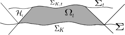
Figure 1: geometric construction used to define the set $\Omega_{t}$ (in dark grey).

Relation (48) and Stokes theorem entail

$$\int_{\Omega_{t}}d{\mathcal{T}_{abc}}=\int_{\partial{\Omega_{t}}}{\mathcal{T}_{abc}}=\int_{\Sigma_{K,t}}\mathcal{T}_{abc}-\int_{\Sigma_{K}}\mathcal{T}_{abc}+\int_{\mathcal{H}_{t}}\mathcal{T}_{abc}\geq\int_{{\Sigma}_{K,t}}\mathcal{T}_{abc}-\int_{\Sigma_{K}}\mathcal{T}_{abc}\;,$$ (49)

where we used in the last step proposition 43 on the null $\mathcal{H}_{t}$ (note that that proposition implies that the other integrals are positive quantities too). Also, the identity (42) applied to ${\boldsymbol{\omega}}=dt$ enables us to transform the first integral

$$\int_{\Omega_{t}}d{\mathcal{T}_{abc}}=\int_{\Omega_{t}}\varphi\;dt\wedge\mathcal{T}_{abc}=\int_{0}^{t}ds\int_{\Sigma_{K,s}}\varphi\mathcal{T}_{abc}.$$ (50)

Note that all integrals in previous expressions are evaluated over compact sets and therefore their existence is guaranteed. Combining eqs. (49)-(50) we get

$$\int_{\Sigma_{K,t}}\mathcal{T}_{abc}\leq\int_{\Sigma_{K}}\mathcal{T}_{abc}+\int_{0}^{t}ds\int_{\Sigma_{K,s}}\varphi\;\mathcal{T}_{abc}\leq\left(1+\int_{0}^{t}m(s)ds\right)\int_{\Sigma_{K}}\mathcal{T}_{abc}\;,\quad t\in I\;,$$ (51)

where in the last inequality we used (46) and the integrability of $m(t)$. Finally, we note that this estimate holds for any compact $\Sigma_{K,t}\subset\Sigma_{t}$ and that the quantity $m(t)$ is totally independent from the set $\Sigma_{K,t}$ we chose at the beginning. This fact and the assumption that $\int_{\Sigma}\mathcal{T}_{abc}$ exists enables us to conclude that $\int_{\Sigma_{t}}\mathcal{T}_{abc}$ also exists $\forall t\in I$. ∎

Remark 1.

If we let $\Sigma_{K}$ approach $\Sigma$ then (51) becomes

$$\int_{\Sigma_{t}}\mathcal{T}_{abc}\leq\left(1+\int_{0}^{t}m(s)ds\right)\int_{\Sigma}\mathcal{T}_{abc}\;,\quad t\in I.$$ (52)

Using proposition 43 we deduce that the term in brackets must be positive

$$0\leq 1+\int_{0}^{t}m(s)ds.$$ (53)

Remark 2.

We can chose a frame $\sigma$ such that it determines the foliation $\{\Sigma_{t}\}$ of theorem 1 (for example one of the elements of the frame is an integrable vector field which is normal to the leaves of the foliation). Under this provision we can regard the conditions stated by theorem 1 as a set of conditions imposed on a frame (gauge choice). Therefore theorem 1 is a geometric construction of a gauge with interesting properties. These properties may enable us to prove global existence results for the Einstein equations as we explain below.

If the unit normal $\vec{\boldsymbol{n}}$ to the foliation $\{\Sigma_{t}\}$ is an element of the frame $\sigma$, then the estimate (52) can be written in the form

$$0<\int_{\Sigma_{t}}{\mathcal{T}}_{000}\leq\left(1+\int_{0}^{t}m(s)ds\right)\int_{\Sigma}{\mathcal{T}}_{000}\;,$$ (54)

where we chose the label 0 for the frame element associated to $\vec{\boldsymbol{n}}$. The computations carried out in the proof of proposition 43 enable us to re-write the previous equation as follows

$$0<\int_{\Sigma_{t}}{\boldsymbol{T}}(\vec{\boldsymbol{n}},\vec{\boldsymbol{n}},\vec{\boldsymbol{n}},\vec{\boldsymbol{n}})d{\Sigma_{t}}\leq\left(1+\int_{0}^{t}m(s)ds\right)\int_{\Sigma}{\boldsymbol{T}}(\vec{\boldsymbol{n}},\vec{\boldsymbol{n}},\vec{\boldsymbol{n}},\vec{\boldsymbol{n}})d\Sigma.$$ (55)

The scalar ${\boldsymbol{T}}(\vec{\boldsymbol{n}},\vec{\boldsymbol{n}},\vec{\boldsymbol{n}},\vec{\boldsymbol{n}})$ is the so-called superenergy density and from the considerations coming after the proof of proposition 28 we deduce that it is a strictly positive quantity which is zero if and only if the Weyl tensor is zero. Therefore we can regard the integrals appearing in equation (55) as a measure of the strength of the gravitational field on $\Sigma$ and $\Sigma_{t}$. The mathematical properties of the superenergy density have been used successfully in the proof of a number of mathematical results [3, 11, 12, 6, 5] and we expect that the estimate shown in (55) will be useful to prove global existence results for the equations of any gravitational theory by means of a standard bootstrap argument (see e.g. [22]). If there exists a frame choice (gauge choice) $\sigma$ in which the assumptions of theorem 1 hold with $\mathcal{T}_{abc}$ as the superenergy density then we deduce from these results that any local existence result for any gravitational theory formulated in the gauge $\sigma$ could be turned into a global one. The idea is to construct inital data in which the condition (45) is fulfilled because then (55) implies that the solution will be regular and bounded if $t\in I$ where $I$ represents the local existence interval. If it turns out that the function $m(t)$ is integrable on $\mathbb{R}$ (or an unbounded subset thereof) then it is plausible that the solution can be extended by using repeatedly the local existence result and theorem 1 thus showing that the solution remains bounded and regular in the maximal data development. In this sense it is important to formulate a local existence result in a gauge $\sigma$ and a foliation with the properties stated by theorem 1. This is the subject of ongoing work.

6 Conclusions

We have shown that one can construct conserved currents involving the classical Bel-Robinson tensor and other superenergy tensors in a manner which appears to be new. These conserved currents contain also a pseudo tensorial part in a pretty much the same way as it happens when one considers conserved currents involving the energy-momentum tensor of the matter. As far as we are aware of, this is the first time that the pseudo-tensorial character of the superenergy is considered in the literature. We have shown that the conservation of superenergy adopts the form of a geometric identity which bears a formal similarity to the Sparling identity. In the latter case the energy of the matter enters in the identity via the Einstein equations whereas no counterpart to the Einstein equations exists in the conservation of the superenergy (there is no known dynamics for the superenergy). For this reason the conservation of the superenergy put forward in this paper should be regarded at this stage as a mathematical result rather than a physical law. An independent physical law of the conservation of the superenergy would exist if one could relate in a physical fashion the superenergy tensors $K_{abcd}$ and $T_{abcd}$ to other superenergy tensors constructed from matter fields (for example the Chevreton tensor [4] or similar). Of course we can always compute $K_{abcd}$ and $T_{abcd}$ for a solution of the Einstein equations and speak of the conservation of superenergy within the framework of the present work. However, in this particular case the conservation of superenergy is a derived law rather than an independent one. We have also explored an independent application involving the construction of an estimate of the causal components of the Bel-Robinson tensor with respect to a frame with certain properties. This estimate could be important in the proof of global existence results of arbitrary gravitational theories, not necessarily based on the classical Einstein equations. Finally we should mention that our work has been restricted to dimension four. A possible generalisation to higher dimensions is under current research.

References

- [1] L. Bel, Sur la radiation gravitationnelle, C. R. Acad. Sci. Paris 247 (1958), 1094–1096.
- [2] G. Bergqvist, I. Eriksson, and J. M. M. Senovilla, New electromagnetic conservation laws, Classical Quantum Gravity 20 (2003), no. 13, 2663–2668.
- [3] M. A. G. Bonilla and J. M. M. Senovilla, Very Simple Proof of the Causal Propagation of Gravity in Vacuum, Phys. Rev. Lett. 78 (1997), no. 5, 783–786.
- [4] M. Chevreton, Sur le tenseur de superénergie du champ électromagnétique, Nuovo Cimento (10) 34 (1964), 901–913.
- [5] D. Christodoulou, The formation of black holes in general relativity, EMS Monographs in Mathematics, European Mathematical Society (EMS), Zürich, 2009.
- [6] D. Christodoulou and S. Klainerman, The global nonlinear stability of the Minkowski space, Princeton Mathematical Series, vol. 41, Princeton University Press, Princeton, NJ, 1993.
- [7] M. Dubois-Violette and J. Madore, Conservation laws and integrability conditions for gravitational and Yang-Mills field equations, Comm. Math. Phys. 108 (1987), no. 2, 213–223.
- [8] Ingemar Eriksson, Conserved matter superenergy currents for hypersurface orthogonal Killing vectors, Classical Quantum Gravity 23 (2006), no. 7, 2279–2290.
- [9] , Conserved matter superenergy currents for orthogonally transitive abelian isometry groups, Classical Quantum Gravity 24 (2007), no. 20, 4955–4968.
- [10] Jörg Frauendiener, Geometric description of energy-momentum pseudotensors, Classical Quantum Gravity 6 (1989), no. 12, L237–L241.
- [11] A. García-Parrado, Dynamical laws of superenergy in general relativity, Class. Quantum. Grav. 25 (2008), no. 1, 015006,26.
- [12] A. García-Parrado and J. A. Valiente Kroon, Kerr initial data, Classical Quantum Gravity 25 (2008), no. 20, 205018, 20.
- [13] S. W. Hawking and G. F. R. Ellis, The large scale structure of space-time, Cambridge University Press, Cambridge, 1973.
- [14] S. Klainerman and F. Nicolò, The evolution problem in general relativity, Progress in Mathematical Physics, vol. 25, Birkhäuser Boston Inc., Boston, MA, 2003.
- [15] S. Kobayashi and K. Nomizu, Foundations of differential geometry. Vol. I, Wiley Classics Library, John Wiley & Sons Inc., New York, 1996, Reprint of the 1963 original, A Wiley-Interscience Publication.
- [16] Ruth Lazkoz, José M. M. Senovilla, and Raül Vera, Conserved superenergy currents, Classical Quantum Gravity 20 (2003), no. 19, 4135–4152.
- [17] J. M. Martín-García, xAct: efficient tensor computer algebra, http://www.xact.es.
- [18] V. Moncrief, An integral equation for spacetime curvature in general relativity, Surveys in differential geometry. Vol. X, Surv. Differ. Geom., vol. 10, Int. Press, Somerville, MA, 2006, pp. 109–146.
- [19] J. M. M. Senovilla, Singularity Theorems and Their Consequences, Gen. Rel. Grav. 29 (1997), no. 5, 701–848.
- [20] , Super-energy tensors, Class. Quantum Grav. 17 (2000), no. 14, 2799–2841.
- [21] László. B. Szabados, On canonical pseudotensors, Sparling’s form and Noether currents, Class. Quantum Gravity 9 (1992), no. 11, 2521–2541.
- [22] T. Tao, Nonlinear Dispersive Equations, Regional Conference Series in Mathematics, no. 106, American Mathematical Society, 2006.