Scale-free and multifractal time dynamics of fMRI signals during rest and task

Abstract

Scaling temporal dynamics in functional MRI (fMRI) signals have been evidenced for a decade as intrinsic characteristics of ongoing brain activity [76]. Recently, scaling properties were shown to fluctuate across brain networks and to be modulated between rest and task [40]: Notably, Hurst exponent, quantifying long memory, decreases under task in activating and deactivating brain regions. In most cases, such results were obtained: First, from univariate (voxelwise or regionwise) analysis, hence focusing on specific cognitive systems such as Resting-State Networks (RSNs) and raising the issue of the specificity of this scale-free dynamics modulation in RSNs. Second, using analysis tools designed to measure a single scaling exponent related to the second order statistics of the data, thus relying on models that either implicitly or explicitly assume Gaussianity and (asymptotic) self-similarity, while fMRI signals may significantly depart from those either of those two assumptions [25, 74].

To address these issues, the present contribution elaborates on the analysis of the scaling properties of fMRI temporal dynamics by proposing two significant variations. First, scaling properties are technically investigated using the recently introduced Wavelet Leader-based Multifractal formalism (WLMF) [73, 3]. This measures a collection of scaling exponents, thus enables a richer and more versatile description of scale invariance (beyond correlation and Gaussianity), referred to as multifractality. Also, it benefits from improved estimation performance compared to tools previously used in the literature. Second, scaling properties are investigated in both RSN and non-RSN structures (e.g., artifacts), at a broader spatial scale than the voxel one, using a multivariate approach, namely the Multi-Subject Dictionary Learning (MSDL) algorithm [68] that produces a set of spatial components that appear more sparse than their Independent Component Analysis (ICA) counterpart.

These tools are combined and applied to a fMRI dataset comprising 12 subjects with resting-state and activation runs [59]. Results stemming from those analysis confirm the already reported task-related decrease of long memory in functional networks, but also show that it occurs in artifacts, thus making this feature not specific to functional networks. Further, results indicate that most fMRI signals appear multifractal at rest except in non-cortical regions. Task-related modulation of multifractality appears only significant in functional networks and thus can be considered as the key property disentangling functional networks from artifacts. These finding are discussed in the light of the recent literature reporting scaling dynamics of EEG microstate sequences at rest and addressing non-stationarity issues in temporally independent fMRI modes.

1 Introduction

Much of what is known about brain function stems from studies in which a task or a stimulus is administred and the resulting changes in neuronal activity and behaviour are measured. From the advent of human electroencephalography (EEG) to cognitive activation paradigms in functional Magnetic Resonance Imaging (fMRI), this approach proved very successful to study brain function, and more precisely functional specialization in human brain. It has relied, on one hand, on contrasting signal magnitude between different experimental conditions [58] or task-specific hemodynamic response (HRF) shape [29] and, on other-hand, on statistical methods often framed within linear or bilinear modelling strategies [37, 49, 50].

Spontaneous modulations of neural activity in Blood Oxygenation Level Dependent (BOLD) fMRI signals however arise without external input or stimulus and thus depict intrinsic brain activity [30]. This ongoing activity constitutes a major part of fMRI recordings and is responsible for most of brain energy consumption. It has hence been intensively studied over the last decade using various methods ranging from univariate, i.e., Seed-based linear Correlation Analysis (SCA) [11, 39], to multivariate methods such as Independent Component Analysis (ICA) [19, 10], group-level ICA [27, 70] or more recent dictionary learning techniques [68]. All these methods have revealed that interactions between brain regions, also referred to as functional connectivity, occur through these spontaneous modulations and consistantly vary between rest and task [30, 36]. Resting-State Network (RSN) extraction from resting-state fMRI time series is thus achieved either by thresholding the correlation matrix computed between voxels or regions (seed-based or univariate approach) or by identifying spatial maps in ICA-based algorithms that closely match RSNs such as somato-sensory systems (visual, motor, auditory), the default mode and attentional networks (ventral and dorsal) [36, 63]. For a recent review about the pros and cons of the SCA and ICA approaches to RSN extraction, the reader can refer to [27]. Once RSNs are extracted, their topological properties can be analyzed with respect to small-world or scale-free models [23, 33, 77, 14].

In parallel and alternatively to brain topology, the temporal dynamics of brain activity have also been extensively studied. It is now well accepted that brain activity, irrespective of the imaging technique involved in observation, is always arrhythmic and shows a scaling, or scale invariant or scale-free, time dynamics, which implies that no time scale plays a predominant or specific role. Often, scale invariance or scale-free dynamics is associated with long range correlation in time [47, 65, 67], and accordingly, in the frequency domain, related to a power-law decrease of the power spectrum ($\Gamma(f)\!\!\propto\!\!1/f^{\beta}$ with $\beta\!>\!0$) in the limit of small frequencies ($f\!\rightarrow\!0$). Interestingly, it is generally admitted that only low frequencies ($<0.1$Hz) convey information related to neural connectivity in fMRI signals [28, 46, 5]. Evidence of fractal or scale-free behavior in fMRI signals has been demonstrated for a long while [76, 13, 15] though it was initially regarded as noise. Deeper investigations of the temporal scale-free property in fMRI have demonstrated that this constitutes an intrinsic feature of ongoing brain activity (cf. e.g. [66, 62, 54, 25, 74, 41, 40]). First attempts to identify stimulus-induced signal changes from scaling parameters were proposed in [66, 62], where a voxel-based fluctuation analysis was applied to high temporal resolution fMRI data. Interestingly, fractal features of voxel time series have enabled to discriminate white matter, cerebrospinal fluid and active from inactive brain regions during a block paradigm [62]. Further, it was shown that scaling properties can be modulated in neurological disorder [54] or between rest and task [66, 62, 25, 74, 40]: It was shown that long memory, as quantified by the Hurst exponent, decreases during task in activating and deactivating brain regions. Analyzing scale invariance in temporal dynamics may thus provide new insights into how the brain works by mapping quantitative estimations of parameters with good specificities to cognitive states, task performance [62, 74, 41, 40].

Small world and scale-free topology led to model brain as a complex critical system, that is as a large conglomerate of interacting components, with possibly nonlinear interactions [8, 24]. Further, these complex systems were then regarded as potential origins for long-range correlation spatio-temporal patterns, as critical systems, i.e., complex systems driven close to their phase transitions, constitute known mechanism yielding scaling time dynamics and generic $1/f$ power spectral densities (see e.g. [24]). They however so far failed to account for the existence of possibly richer scaling properties (such as e.g., multifractality). At a general level, scale invariance in time dynamics and scale-free property of brain topology are, in essence, totally independent properties that must not be confused one with the other. Whether or not and how these two scale-free instances are related one to the other in the fMRI context remains a difficult and largely unsolved issue, far beyond the scope of the present contribution, that concentrates instead on performing a thorough analysis of scale invariance temporal dynamics in fMRI signals.

In the existing literature, the analysis of scale invariance in fMRI signals suffers from two limitations: First, it has often been performed at the voxel or region level, thus consisting of a collection of univariate analyses, suffering from the classical bias of voxel selection or region definition. Moreover, although the fluctuation of scale-free dynamics with tissue type has been studied in [62, 74] to derive that stronger persistency occurs in grey matter and that this background activity might represent neuronal dynamics, no systematic analysis has been undertaken to disentangle the scale-free properties of RSN and non-RSN components, such as artifacts. This investigation can be better handled using multivariate or ICA-like approaches. Second, scale invariance in fMRI signals has mostly been based on spectral analysis and/or Detrended Fluctuation Analysis (cf. e.g. [66, 65, 40]). This amounts to considering that scaling is associated only with the correlation or the spectrum (hence with the second order statistics) of the data and thus, implicitly and sometimes even explicitly, to assuming Gaussianity and (asymptotic) self-similarity for the data (cf. e.g. [34] for a survey in the fMRI context). Also, it is now well-known that such technics lack robustness to disentangle stationarity/non-stationarity versus true scaling property issues and do not allow simple extension to account for richer scaling properties such as those observed in multifractal models. It is well-accepted that wavelet analysis based analysis of scaling (cf. e.g. [2, 4, 71, 13, 35]) yield not only better estimation performance, but also show significant practical robustness, notably to non-stationarity, while paving the way toward the analysis of scaling properties beyond the strict second-order (hence beyond Gaussianity and asymptotic self-similarity).

In this context, the present contribution elaborates on earlier works dedicated to the analysis of scale invariance in fMRI temporal dynamics by proposing two significant variations.

First, scale invariance dynamics is not investigated at the voxel or region spatial scale level independently. Instead, group-level resting-state networks are segmented by an exploratory multivariate decomposition approach, namely the MSDL algorithm [68], detailed in Section 3: It produces both a set of spatial components and a set of times series, for each component and each subject, that conveys ongoing dynamics in functional networks but also in artifacts. As shown in [68], the sparsisty promoting regularization involved in the MSDL algorithm enables to recover less noisy spatial maps than group-level or canonical ICA [70]. This makes their interpretation easier in the context of small group of individuals. This technique is detailed in Section 3.

Second, to enable an in-depth analysis of the scaling properties of the temporal dynamics in fMRI signals, we resort to multifractal analysis, that measures not a single but a collection of scaling exponents, thus enabling a richer and more versatile description of scale invariance (beyond correlation and Gaussianity), referred to as multifractality. It is thus likely to better account for the variety and complexity of potential scaling dynamics, as already suggested in the context of fMRI in e.g. [25, 74]. However, in contrast to [74], and following the track opened in [25], we use a recent statistical analysis tool, the Wavelet Leader-based Multifractal formalism (WLMF) [73, 3]. This formalism benefits from better mathematical grounding and shows improved estimation performance compared to tools previously used in the literature. This framework is introduced in Section 4, after a review of the intuition, models and methodologies underlying the definition and analysis of scaling temporal dynamics, thus, to some extend, continuing and renewing the surveys provided in [34, 25].

These tools are combined together and applied to two datasets, corresponding to resting-state and activation runs. They are described in Section 2 (see also [59]). Modulations of scale-free and multifractal properties in space, i.e., between functional and artifactual components but also between rest and task, are statistically assessed at the group level in Section 5.

In agreement with findings in [40], the results reported here confirm that fMRI signals can be modeled as stationary processes, as well as the decrease of the estimated long memory parameter under task. However, this is found to occur everywhere in the brain and not specifically in functional networks. Moreover, evidence for multifractality in resting-state fMRI signals is demonstrated except for non-cortical regions. Task-related modulations of multifractality appear only significant in functional networks and thus become the key property to disentangle functional networks from artefacts. However, in contrast to what happens for the long memory parameter, this modulation is not monotonous across the brain and varies between cortical and non-cortical regions. These results are further discussed in Section 6 in the light of recent findings related to scale-free dynamics of EEG microstate sequences and non-stationarity of functional modes. Conclusions are drawn in Section 7.

2 Data acquisition and analysis

2.1 Data acquisition

Twelve right-handed normal-hearing subjects (two female; ages, 19–30) gave written informed consent before participation in an imaging study on a 3T MRI whole-body scanner (Tim-Trio; Siemens). The study received ethics committee approval by the authorities responsible for our institution. Anatomical imaging used a T1-weighted magnetization-prepared rapid acquisition gradient echo sequence [176 slices, repetition time (TR) 2300 ms, echo time (TE) 4.18 ms, field of view (FOV) 256, voxel size $1\!\!\times\!\!1\!\!\times\!\!1$mm³). Functional imaging used a $\text{T2}^{*}$-weighted gradient-echo, echo-planar-imaging sequence (25 slices, $\text{TR}\!\!=\!\!1500$ ms, $\text{TE}\!\!=\!\!30$ ms, FOV 192, voxel size $3\!\!\times\!\!3\!\!\times\!\!3$mm³). Stimulus presentation and response recording used the Cogent Toolbox (John Romaya, Vision Lab, UCL) for Matlab and sound delivery a commercially available MR-compatible system (MR Confon).

The rs-fMRI dataset we consider in this study has already been published in [59]. 820 volumes of task-free “resting state” data (with closed, blind-folded eyes) were acquired before getting experimental runs of 820 volumes each. These experimental runs, which have not been analyzed in [59], involve an auditory detection task (run 2, motor response), and make use of a sparse supra-threshold auditory stimulus detection.

The auditory stimulus was a 500 ms noise burst with its frequency band modulated at 2 Hz (from white noise to a narrower band of 0–5 kHz and back to white noise). Inter-stimulus intervals ranged unpredictably from 20 to 40 s, with each specific interval used only once. Subjects were instructed to report as quickly and accurately as possible by a right-hand key press whenever they heard the target sound despite scanner’s background noise. Details about the definition of each subject’s auditory threshold are available in [59].

2.2 Data analysis

We used here statistical parametric mapping (SPM5, Wellcome Department of Imaging Neuroscience, UK. for image preprocessing (realignment, coregistration, normalization to MNI stereotactic space, spatial smoothing with a 5 mm full-width at half-maximum isotropic Gaussian kernel for single-subject and group analyses) and our own software developments for subsequent analyses. More precisely, the MSDL algorithm relies on the scikit-learn Python toolbox and the multifractal analysis on the WLBMF Matlab toolbox.

3 Multivariate decomposition of resting state networks

3.1 Multisubject spatial decomposition techniques

The fMRI signal observed in a voxel reflects many different processes, such as cardiac or respiratory noise, movement effects, scanner artifacts, or the BOLD effect that reveals the underlying neural activity of interest. We separate these different contributions making use of a recently introduced multivariate analysis technique that estimates jointly spatial maps and time series characteristic of these different processes [68]. Formally, this estimation procedure amounts to finding $K$ spatial maps ${\mathb{V}}_{s}\in\mathbb{R}^{p\times K}$ and the corresponding time series ${\mathb{U}}_{s}\in\mathbb{R}^{n\times K}$, whose linear combination fits well the observed brain signals, ${\mathb{Y}}_{s}\in\mathbb{R}^{n\times p}$, of length $n$, measured over $p$ voxels, for subject $s$:

$$\qquad{\mathb{Y}}_{s} ={\mathb{U}}_{s}{\mathb{V}}_{s}^{\mathrm{t}}+{\mathb{E}}_{s},$$ (1)

with ${\mathb{E}}_{s}\in\mathbb{R}^{n\times p}$ the subject-level noise, or residuals not explained by the model. Finding ${\mathb{V}}_{s}^{\mathrm{t}}$ enables the separation of the contributions of the different process that are mixed at the voxel level, but implies to work on spatial maps rather than on specific voxels. The number of spatial maps, $K$, is not chosen a priori, but selected by the procedure.

This problem can be seen as a blind source separation task in the presence of noise, and has often been tackled in fMRI using ICA, combined with principal component analysis (PCA) to reject noise [55, 44, 10]. In the multi-subject configuration, estimating the spatial maps on all subjects simultaneously makes it easy to relate the factors estimated across the different subjects. This can be done by concatenating the data across subject, modeling a common distribution [19], or by extending the data-reduction step performed in the PCA by a second level capturing inter-subject variability [70]. More recently, it was proposed that the key to the success of ICA on fMRI data, is to recover sparse spatial maps [31, 69]. This hypothesis can be formulated as a sparse prior in model (1), which can then be estimated using sparse PCA or sparse dictionary learning procedures. With regards to our goal in this study, extracting time-series specific to the various processes observed, a strong benefit of such procedures is that they can perform data reduction, i.e., estimation of the residuals not explained by the model, and extraction of the relevant signals in a single step informed by our prior. On the opposite, with ICA-based procedures, the residuals are selected by the PCA step, and not the ICA step.

3.2 Multi-subject Dictionary Learning algorithm

In addition, Varoquaux et al. [68] have adapted the dictionary learning procedures to a multi-subject setting, in a so-called multi-subject dictionary learning (MSDL) framework. On fMRI datasets, the procedure extracts a group-level atlas of spatial signatures of the processes observed, as well as corresponding subject-level maps, accounting for the individual specificities. They show that, with a small spatial smoothness prior added to the sparsity prior on the maps, the extracted patterns correspond to the segmentation of various structures in the signal: functional regions, blood vessels, interstitial spaces, sub-cortical structures… In these settings, the subject-level maps ${{\mathb{V}}_{s}}$ are modeled as generated by group-level maps ${\mathb{V}}\in\mathbb{R}^{p\times K}$ with additional inter-subject variability that appears as residual terms, ${\mathb{F}}_{s}\in\mathbb{R}^{p\times K}$, at the group level:

$\displaystyle\forall s\in\left\{1,\,\ldots,\,S\right\},\>{\mathb{V}}_{s}={\mathb{V}}+{\mathb{F}}_{s}.$

The model is estimated by finding the group-level and subject-level maps that maximize the probability of observing the data at hand with the given prior. This procedure is known as a Maximum A Posteriori (MAP) estimate, and boils down to minimizing the negated log-likelihood of the model with an additional penalizing term. If the two sources of unexplained signal, i.e. subject-level residuals ${\mathb{E}}_{s}$ and inter-subject variability ${\mathb{F}}_{s}$ are modeled as Gaussian random variates, the log-likelihood term is the sum of squares of these errors. The prior term appears as the sum of the sparsity-inducing $\ell_{1}$ norm of ${\mathb{V}}$, and the $\ell_{2}$ norm of the gradient of the map, enforcing the smoothness. This prior has been used previously in regression settings under the name of smooth-Lasso [42]. Estimating the model from the data thus consists of minimizing the following criterion:

$\displaystyle{\mathcal{J}}({\mathb{U}}_{s},{\mathb{V}}_{s},{\mathb{V}})=\sum_{s=1}^{S}\bigl{(}\|{\mathb{Y}}_{s}-{\mathb{U}}_{s}{\mathb{V}}_{s}^{\mathrm{t}}\|^{2}+\mu\|{\mathb{V}}_{s}-{\mathb{V}}\|^{2}\bigr{)}$

$\displaystyle+\lambda\,\bigl{(}\|{\mathb{V}}\|_{1}+{\mathb{V}}^{\mathrm{t}}{\mathb{L}}\,{\mathb{V}}/2\bigr{)}$

where, $\|{\mathb{V}}\|_{1}$ is the $\ell_{1}$ norm of ${\mathb{V}}$, i.e the sum the absolute values, ${\mathb{L}}$ is the image Laplacian – ${\mathb{V}}^{\mathrm{t}}{\mathb{L}}\,{\mathb{V}}$ is the norm of the gradient. $\lambda$ is a parameter controlling the amount of prior set on the maps, and thus the amount of sparsity, that is set by Cross-Validation (CV). $\mu$ is a parameter controlling the amount of inter-subject validation, that is set by comparing intra-subject variance in the observations with inter-subject variance. For more details about the estimation procedure or the parameter setting, we refer the reader to [68].

3.3 Resting state MSDL maps

rs-fMRI runs were analyzed for $S=12$ subjects, consisting of $n=820$ volumes (time points) with a $3\,\text{mm}$ isotropic resolution, corresponding to approximately $p=50\,000$ voxels within the brain. The automatic determination rule of the number of maps exposed in [69] converges to $K=42$. Also, the CV procedure gives us the best CV criterion for $\lambda=2$. The group-level maps ${\mathb{V}}$ are shown in Fig. 1. They have been manually classified in three groups: Functional (F), Artifactual (A) and Undefined (U) maps that appear color-coded in red, blue and green, respectively. The undefined class appeared necessary to introduce some confidence measure in our classification and disambiguate well-established networks (e.g., dorsal attentional network) from inhomogenous components mixing artifacts with neuronal regions  (e.g. like in ${\mathb{v}}_{9}$). The anatomo-functional description of these group-level maps and their class assignment is given in Table 1. The same rules applied for individual maps ${\mathb{V}}_{s}$. In what follows, we will denote by $\mathcal{F}$, $\mathcal{A}$ and $\mathcal{U}$ the index sets of F/A/U-maps, respectively and by ${\mathrm{Card}}\left({\mathcal{F}}\right)=25$, ${\mathrm{Card}}\left({\mathcal{A}}\right)=13$ and ${\mathrm{Card}}\left({\mathcal{U}}\right)=4$ their respective size.

Figure 1: From left to right and top to bottom, group-level MSDL maps ${\mathb{V}}=\left[{\mathb{v}}_{1}\,|\,\cdots\,|\,{\mathb{v}}_{42}\right]$ inferred from the multisubject ($S=12$) resting-state fMRI dataset (Neurological convention: left is left). Functional (F), Artifactual (A) and Undefined (U) maps appear color-coded boxes in red, blue and green, respectively. Let us denote $\mathcal{F}$, $\mathcal{A}$ and $\mathcal{U}$ the index sets of F/A/U-maps, respectively and ${\mathrm{Card}}\left({\mathcal{F}}\right)=25$, ${\mathrm{Card}}\left({\mathcal{A}}\right)=13$ and ${\mathrm{Card}}\left({\mathcal{U}}\right)=4$ their respective size. Each map ${\mathb{v}}_{k}$ consists of loading parameters within the $(-1,1)$ range where positive and negative values are depicted by the hot and cold parts of the colorbar.

Table 1: Classification of group-level ${\mathb{V}}=\left[{\mathb{v}}_{1}\,|\,\cdots\,|\,{\mathb{v}}_{42}\right]$ maps according to the F/A/U labelling. The F-maps have been subdivided in different functional networks: Attentional, Default Mode Network, Motor, Visual. Basal Ganglia (Thalamus, Caudate and Putamen) and cerebellum have been put together under the Non cortical label. They will be considered together in the following set: ${\mathcal{N}}=\left\{\text{Att},\text{DMN},\text{Mot},\text{N-c},\text{Vis}\right\}$. The artifacts have been distinguished in four types: Ventricles, White Matter, Movement and Other. The corresponding set will be denoted ${\mathcal{T}}=\left\{\text{Ven},\text{WhM},\text{Mov},\text{Oth}\right\}$.

Index	Anatomo-functional description	Label	Network
${\mathb{v}}_{1}$	Ventral primary sensorimotor cortex	F (${\mathb{f}}_{1}$)	Mot.
${\mathb{v}}_{2}$	Dorsal primary motor cortex or edge of recorded volume	U (${\mathb{u}}_{1}$)
${\mathb{v}}_{3}$	Midbrain	A (${\mathb{a}}_{1}$)	Oth.
${\mathb{v}}_{4}$	Precuneus, posterior cingulate cortex	F (${\mathb{f}}_{2}$)	DMN
${\mathb{v}}_{5}$	Calcarine cortex (V1)	F (${\mathb{f}}_{3}$)	Vis.
${\mathb{v}}_{6}$	Anterior cerebellar lobe	F (${\mathb{f}}_{4}$)	N-c
${\mathb{v}}_{7}$	Ventricles	A (${\mathb{a}}_{2}$)	Ven.
${\mathb{v}}_{8}$	Caudate, Thalamus and Putamen	F (${\mathb{f}}_{5}$)	N-c
${\mathb{v}}_{9}$	Pre- and supplementary motor cortex	U (${\mathb{u}}_{2}$)
${\mathb{v}}_{10}$	Occipital cortex	F (${\mathb{f}}_{6}$)	Vis.
${\mathb{v}}_{11}$	Ventricles	A (${\mathb{a}}_{3}$)	Ven.
${\mathb{v}}_{12}$	Median prefrontal cortex	F (${\mathb{f}}_{7}$)	DMN
${\mathb{v}}_{13}$	Right lateralized fronto-parietal cortex	F (${\mathb{f}}_{8}$)	Fr.-par.
${\mathb{v}}_{14}$	Ventricles	A (${\mathb{a}}_{4}$)	Ven.
${\mathb{v}}_{15}$	Superior temporal and inferior frontal gyrus	F (${\mathb{f}}_{9}$)	Lang.
${\mathb{v}}_{16}$	Primary sensorimotor cortex	F (${\mathb{f}}_{10}$)	Mot.
${\mathb{v}}_{17}$	artifact	A (${\mathb{a}}_{5}$)	Oth.
${\mathb{v}}_{18}$	Dorsal occipital cortex	F (${\mathb{f}}_{11}$)	Vis.
${\mathb{v}}_{19}$	Supratemporal cortex	F (${\mathb{f}}_{12}$)	Aud.
${\mathb{v}}_{20}$	Semioval center (white matter)	A (${\mathb{a}}_{6}$)	WhM.
${\mathb{v}}_{21}$	Anterior insula and cingulate cortex	F (${\mathb{f}}_{13}$)
${\mathb{v}}_{22}$	Frontal Eye Fields (FEF), intra-parietal cortex	F (${\mathb{f}}_{14}$)	Att.
${\mathb{v}}_{23}$	Ventral occipital cortex	F (${\mathb{f}}_{15}$)	Vis.
${\mathb{v}}_{24}$	Semioval center (white matter)	A (${\mathb{a}}_{7}$)	WhM.
${\mathb{v}}_{25}$	Lateral occipital cortex	F (${\mathb{f}}_{16}$)	Vis.
${\mathb{v}}_{26}$	Parieto-occipital cortex	F (${\mathb{f}}_{17}$)	Vis.
${\mathb{v}}_{27}$	Extracerebral space	A (${\mathb{a}}_{8}$)	Oth.
${\mathb{v}}_{28}$	Left lateralized ventral fronto-parietal cortex	F (${\mathb{f}}_{18}$)	Fr.-par.
${\mathb{v}}_{29}$	Retrosplenial and anterior occipital cortex	U (${\mathb{u}}_{3}$)
${\mathb{v}}_{30}$	White matter	A (${\mathb{a}}_{9}$)	WhM.
${\mathb{v}}_{31}$	Left lateralized fronto-parietal system	F (${\mathb{f}}_{19}$)	Fr.-par.
${\mathb{v}}_{32}$	Right lateralized ventral fronto-parietal system	F (${\mathb{f}}_{20}$)	Att.
${\mathb{v}}_{33}$	Mesial temporal system	F (${\mathb{f}}_{21}$)
${\mathb{v}}_{34}$	Dorsomedian frontal cortex	F (${\mathb{f}}_{22}$)	DMN
${\mathb{v}}_{35}$	White matter	A (${\mathb{a}}_{10}$)	WhM.
${\mathb{v}}_{36}$	Motion-related artifact	A (${\mathb{a}}_{11}$)	Mov.
${\mathb{v}}_{37}$	Bilateral prefrontal cortex and anterior Caudate	F (${\mathb{f}}_{23}$)
${\mathb{v}}_{38}$	Left lateralized temporo-parietal junction and inferior frontal gyrus	F (${\mathb{f}}_{24}$)	Att.
${\mathb{v}}_{39}$	Right lateralized temporo-parietal junction and inferior frontal gyrus	F (${\mathb{f}}_{25}$)	Att.
${\mathb{v}}_{40}$	Bilateral superior parietal lobe	U (${\mathb{u}}_{4}$)
${\mathb{v}}_{41}$	White matter	A (${\mathb{a}}_{12}$)	WhM.
${\mathb{v}}_{42}$	artifact	A (${\mathb{a}}_{13}$)	Oth.

To compare spontaneous and evoked activity, the same spatial decomposition was used on resting-state (run 1, Rest) and task-related data, which were acquired during an auditory detection task (run 2, Task). In practice, this consists of projecting the task-related fMRI data $\widetilde{{\mathb{Y}}}_{s}$ onto the inferred spatial maps ${\mathb{V}}_{s}$ by minimizing the following least square criterion, $\|\widetilde{{\mathb{Y}}}_{s}-{\mathb{W}}_{s}{\mathb{V}}_{s}^{\mathrm{t}}\|^{2}$, with respect to ${\mathb{W}}_{s}$. The time series solution admits a closed-form expression: $\widetilde{{\mathb{U}}}_{s}=\widetilde{{\mathb{Y}}}_{s}{\mathb{V}}_{s}\bigl{(}{\mathb{V}}_{s}^{\mathrm{t}}{\mathb{V}}_{s}\bigr{)}^{-1}$. The subsequent scale-free analysis is applied to the two sets of $n\times K$ map-level fMRI time series ${\mathb{U}}_{s}=\left[{\mathb{u}}_{s,1}\,|\,\ldots\,|\,{\mathb{u}}_{s,K}\right]^{\mathrm{t}}$ and $\widetilde{{\mathb{U}}}_{s}=\left[\widetilde{{\mathb{u}}}_{s,1}\,|\,\ldots\,|\,\widetilde{{\mathb{u}}}_{s,K}\right]^{\mathrm{t}}$ in a univariate manner, that is to each time series ${\mathb{u}}_{s,k}$ and $\widetilde{{\mathb{u}}}_{s,k}$ for Rest and Task, respectively.

4 Scale-free: Intuition, models and analyses

4.1 Intuition

In the analysis of evoked brain activity, it is common to seek correlations of BOLD signals with any a priori shape of the hemodynamic response convolved with the experimental paradigm. In the frequency domain, this amounts to seeking response energy concentration in pre-defined spectral bands, as induced for instance by periodic stimulation (e.g. flashing checkerboards). In resting-state fMRI, it is now well admitted that intrinsic brain activity is characterized by scale-free properties [76, 40]. This constitutes a major change in paradigm as it implies that brain activity is not to be analyzed via the amounts of energy it shows within specific and a priori chosen frequency bands, but instead via the fact that all frequencies are jointly contributing in an equivalent manner to its dynamics. Scale-free dynamics are usually described in the spectral domain by a power-law decrease: Let $Y(t)$ denote the signal quantifying brain activity and $\Gamma_{Y}(f)$ its Power Spectral Density (PSD). Scale-free property is classically envisaged as:

$${\mathcal{M}}_{0}:\, \Gamma_{Y}(f)\simeq C|f|^{-\beta},\,\beta\geq 0,$$ (2)

with $f_{m}\leq|f|\leq f_{M},\,\,f_{M}/f_{m}\gg 1$. Such a power law behavior over a broad range of frequencies implies that no frequency in that range plays a specific role, or equivalently, that they are all equally important. To analyze brain activity, this power law relation thus becomes a more important feature than the energy measured at some specific frequencies. For instance, it implies that energy at frequency $f_{1}$ can be deduced from energy at frequency $f_{2}$ according to [40]:

$$\Gamma_{Y}(f_{2}) =\Gamma_{Y}(f_{1})\left(|f_{2}|/|f_{1}|\right)^{-\beta}.$$ (3)

In the scale-free framework, one therefore tries to quantify brain activity by considering the scaling exponent $\beta$ (or variants) as the key descriptor. Let us moreover note that the terminology scale-free is equivalent to scale invariance or simply scaling, encountered in other scientific fields, where this property has also been found to play a central role (cf. [1, 25, 3]).

4.2 Scale-free models

4.2.1 From Spectrum to Increments

Though appealing, Eqs. (2)–(3) do not provide practitioners with a versatile enough definition of scale-free with respect to real-world data analysis. Indeed, they concentrate only on the second order statistics and hence account neither for the marginal distribution (first order statistics) of the signal $Y$, nor for its higher order dynamics (or dependence structure). For instance, it does not indicate whether data are jointly Gaussian or depart, weakly or strongly, from Gaussianity.

To investigate how to enrich Model ${\mathcal{M}}_{0}$, let us assume for now that $Y$ consists of a stationary jointly Gaussian process, with PSD as in Eq. (2). Equivalently, this implies that the covariance function behaves as $C_{Y}(\tau)\sim\sigma^{2}_{Y}(1+C^{\prime}|\tau|^{-\alpha})$, for $\tau_{m}\leq\tau\leq\tau_{M}$, with $\alpha=1-\beta$. A simple calculation hence shows that ${\mathbb{E}}(Y(t+\tau)-Y(t))^{2}={\mathbb{E}}Y(t+\tau)^{2}+{\mathbb{E}}Y(t)^{2}-2{\mathbb{E}}Y(t+\tau)Y(t)=c_{2}|\tau|^{-\alpha}$. The Gaussianity of $Y$ further implies that $\,\forall q>-1$:

$${\mathbb{E}}|Y(t+\tau)-Y(t)|^{q} =c_{q}|\tau|^{-\frac{q\beta}{2}},\,\,\tau_{m}\leq\tau\leq\tau_{M}.$$ (4)

Defining $X(t)=\int^{t}Y(s)ds$, Eq. (4) straightforwardly implies that, as long as $\tau_{m}\leq\tau_{1},\tau_{2}\leq\tau_{M}$:

$$\bigl{\{}\frac{X(t+\tau_{1})-X(t)}{\tau^{H}_{1}}\bigr{\}}_{t\in\mathbb{R}}\stackrel{{\scriptstyle fdd}}{{=}}\bigl{\{}\frac{X(t+\tau_{2})-X(t)}{\tau^{H}_{2}}\bigr{\}}_{t\in\mathbb{R}},$$ (5)

with $H=(-\alpha/2)=(\beta+1)/2$, and where $\stackrel{{\scriptstyle fdd}}{{=}}$ means equality of all joint finite dimensional distributions: i.e., $(X(t+\tau_{1})-X(t))/\tau^{H}_{1}$ and $(X(t+\tau_{2})-X(t))/\tau^{H}_{2}$ have the same joint distributions. In turn, this implies that $\,\forall q>-1$, such that ${\mathbb{E}}|X(t)|^{q}<\infty$:

$${\mathbb{E}}|X(t+\tau)-X(t)|^{q} =c_{q}|\tau|^{qH},\,\,\tau_{m}\leq\tau\leq\tau_{M},\makebox{ or }$$ (6)

$${\mathbb{E}}|X(t+\tau_{2})-X(t)|^{q}={\mathbb{E}}|X(t+\tau_{1})-X(t)|^{q}\left(\frac{|\tau_{2}|}{|\tau_{1}|}\right)^{qH},$$ (7)

with $\tau_{m}\leq\tau_{1},\tau_{2}\leq\tau_{M}$, which are reminiscent of Eqs. (2)–(3).

4.2.2 Self-Similar processes with stationary increments

Eqs. (6)–(7) turn out to hold not only for jointly Gaussian $1/f$-processes but for a much wider and better defined class, that of self-similar processes with stationary increments, referred to as $H$-sssi processes, and defined as (cf. [60]):

$${\mathcal{M}}_{1}: \quad\{X(t)\}_{t\in\mathbb{R}}\stackrel{{\scriptstyle fdd}}{{=}}\{a^{H}X(t/a)\}_{t\in\mathbb{R}},$$ (8)

$\forall a>0$, $H\in(0,1)$. Essentially, it means that $X$ cannot be distinguished (statistically) from any copy, dilated by scale factor $a>0$, on condition that the amplitude axis is scaled by $a^{H}$. Parameter $H$ is referred to as the self-similarity exponent. A major practical consequence of this definition consists of the fact that Eqs. (6)–(7) hold for all $\tau$ (resp., $\tau_{1},\tau_{2}$).

The central benefit of such a definition is that it does not require the data to be Gaussian but provides both theoreticians and practitioners with a well-defined model. For analysis, fMRI data can hence be envisaged as the increment process $Y(t)=X(t+\tau_{0})-X(t)$ of an $H$-sssi process $X$ (where $\tau_{0}$ is an arbitrary constant chosen to make sense with respect to physiology and data acquisition set up, e.g. $\tau_{0}=\text{TR}$). This constitutes a second model to account for scale-free properties in data, that encompasses the simpler $1/f$-spectrum first model.

Further, if joint Gaussianity is assumed, the model becomes even more precise as the only Gaussian $H$-sssi process $X$ is the so-called fractional Brownian motion (fBm), cf. e.g., [52], hereafter labelled $X(t)\equiv B_{H}(t)$. The corresponding increment process $Y(t)=G_{H}(t)=B_{H}(t+1)-B_{H}(t)$ is termed fractional Gaussian noise (fGn). Additionally, note that it may sometimes constitute a practical and relevant challenging issue to decide whether brain activity is better modelled by the $H$-sssi process $X$ (hence a non stationary process) or by its increment process $Y$ (hence a stationary process) (cf. e.g., [25, 41, 40]).

4.2.3 Multifractal processes

In a number of situations, it has been actually observed on a variety of real-world data of very different nature (cf. e.g., [1, 3] for reviews) that Eq. (6) holds over a wide range of $\tau$s, however, with scaling exponents that depart significantly from the theoretical linear behavior $qH$:

$${\mathbb{E}}|X(t+\tau)-X(t)|^{q} =c_{q}|\tau|^{\zeta(q)},\,\,\tau_{m}\leq\tau\leq\tau_{M}.$$ (9)

The generic behaviors modeled by Eq. (9) can be considered as a practical or operational, definition of scale-free property. Let us note that, by nature, $\zeta(q)$ is necessarily a concave function of $q$ (cf. e.g., [73]).

Scaling exponents $\zeta(q)$ that are strictly concave rule out the use of $H$-sssi process as models. Instead, a broader class should be used, referred to as that of multifractal processes. This is however a large and not-well defined class of processes. For the purposes of this contribution, let us use a particular subclass of multifractal processes defined as fBm subordinated to a multiplicative Compound Poisson cascade:

$${\mathcal{M}}_{2}: \quad X(t):=B_{H}(A(t)),\text{where\>}A(t)=\int^{t}W(s)ds,$$ (10)

with $W(s)$ a multiplicative Compound Poisson cascade (or martingale), such as those defined in [9]. The complete definition of these cascades has been given and studied with details elsewhere and is hence not recalled here (cf. [9, 7, 22]). It is enough to emphasize that they rely on the choice of positive random variables whose moments of order $q$ define the $\zeta(q)$. The process $X$ thus defined satisfies Eq. (9) with strictly convex tunable scaling exponents $\zeta(q)$, has stationary increments $Y$, and has distributions that depart from strict jointly Gaussian laws. Such departures, that may however turn subtle and hard to detect in practice, are precisely quantified by the departure of $\zeta(q)$ from a linear behavior in $q$. The $\zeta(q)$ therefore convey a rich information about data $X$, and hence about $Y$, as they account for the entire dependence structure of the data, hence both to the time dynamic and distributions of data. Their accurate estimation from real-world data therefore naturally constitutes an important practical challenge discussed below.

4.3 Scale-free analysis

4.3.1 From spectrum to wavelet analysis

Assuming that data $Y$ have a power-law spectrum behavior as in Eq. (2), it is natural to rely on spectral estimation to measure $\beta$. A classical tool in spectrum analysis is the Welch estimator that consists in splitting data $Y$ into blocks and in averaging the squared Fourier transforms computed independently over each block. For scale free data, it is hence expected that:

$$\hat{\Gamma}_{Y}(f) =\sum_{k}|\langle Y,g_{f,k}\rangle|^{2}\simeq C|f|^{-\beta},$$ (11)

where the $g_{f,k}=g_{0}(t-k)e^{\imath 2\pi ft}$ are translated into time and into frequency templates of a reference pattern $g_{0}(t)$. This relation can be further used to estimate $\beta$.

It has been shown that wavelet transforms can achieve better performance both in the analysis of scale-free properties in real-world data, and in the estimation of the corresponding scaling parameters (cf. [2, 4, 71]). The discrete wavelet transform (DWT) coefficients of $Y$ are defined as:

$$d_{Y}(j,k) =\displaystyle\int_{\mathbb{R}}Y(t)\;2^{-j}\psi_{0}(2^{-j}t-k)\,dt\equiv\langle Y,\psi_{j,k}\rangle,$$ (12)

where the $\psi_{j,k}=2^{-j}\psi_{0}(2^{-j}t-k)$ consists of templates of a reference pattern $\psi_{0}$ translated in time and dilated (by a factor $a=2^{j}$). It is referred to as the mother-wavelet: an elementary function, characterized by fast exponential decays in both the time and frequency domains, as well as by a strictly positive integer $N_{\psi}\geq 1$, the number of vanishing moments, defined as $\forall k=0,1,\ldots,N_{\psi}-1$, $\int_{\mathbb{R}}t^{k}\psi_{0}(t)dt\equiv 0$ and $\int_{\mathbb{R}}t^{N}\psi_{0}(t)dt\neq 0$. Note the choice of the $L^{1}$-norm (as opposed to the more common $L^{2}$-norm choice) that better matches scaling analysis. For further introduction to wavelet transforms, the reader is referred to e.g., [51].

Defining $S^{d}_{Y}(j,2)={1\over n_{j}}\sum_{k=1}^{n_{j}}|d_{Y}(j,k)|^{2}$ (with $n_{j}$ the number of $d_{X}(j,k)$ available at scale $2^{j}$), one obtains (cf. [2]):

$${\mathbb{E}}S^{d}_{Y}(j,2) =\displaystyle\int_{\mathbb{R}}\Gamma_{Y}(f)|{\Psi}_{0}(2^{j}f)|^{2}df$$ (13)

where ${\Psi}_{0}$ denotes the Fourier transform of $\psi_{0}$. This indicates that $S^{d}_{Y}(j,2)$ can be read as a wavelet based estimate of the PSD and is hence referred to as the wavelet spectrum. It measures the amount of energy of $Y$ around the frequency $f_{j}=f_{0}/2^{j}$ where $f_{0}$ is a constant that depends on the explicit choice of $\psi_{0}$ (for the Daubechies wavelet used here, $f_{0}\simeq 3f_{s}/4$ with $f_{s}$ the sampling frequency). This correspondence between the Fourier and wavelet spectra is illustrated on fMRI signals in Fig. 2. For scale-free processes satisfying Eq. (2), it implies:

$$S^{d}_{Y}(j,2)\equiv{1\over n_{j}}\sum_{k=1}^{n_{j}}|\langle Y,\psi_{j,k}\rangle|^{2}\simeq C_{2}2^{j(\beta-1)},\,\,a_{m}\leq 2^{j}\leq a_{M}.$$

While this formally looks like Eq. (11), it has been shown in detail how and why the wavelet spectrum yields better estimates of the scaling exponents $\beta$ than Welch based-ones, both in terms of estimation performance and robustness to various forms of non-stationarity in data that may be confused with scale-free behaviors [2, 4, 71]. Notably, it was shown how wavelet analysis enables to disentangle non stationarity, stemming from fMRI environment, from true long memory in brain activity. Also, the wavelet spectrum avoids the potentially difficult issue that consists of deciding a priori whether empirical data are better modeled by $Y$ or $X$, needed by classical spectrum estimation, that can only be applied to stationary data. In a nutshell, these benefits stem from the use of the change of scale operator to design the analysis tool, that intuitively matches scale-free behavior more naturally than a frequency shift operator.

4.3.2 From 2nd to other statistical orders: Wavelet leaders

As discussed in Section 4.2, analyzing in-depth scale free properties implies investigating not only the spectrum (i.e., the second order statistics of data) but rather the entire dependence structure, i.e., the whole range of available statistical orders $q$. It had initially been thought that this would amount to extending the definition of $S^{d}_{Y}(j,2)$ to other orders $q$, $S^{d}_{Y}(j,q)\equiv{1\over n_{j}}\sum_{k=1}^{n_{j}}|\langle Y,\psi_{j,k}\rangle|^{q}$. It has however recently been shown that this approach, though intuitive and appealingly simple, fails to yield satisfactory estimation of the $\zeta(q)$. Notably, wavelet coefficients show little power in enabling practitioners to decide whether $\zeta(q)$ is a linear or strictly concave function of $q$. Instead, it is now well documented that the estimation of the $\zeta(q)$ should be based on Wavelet Leaders [73].

Let us now assume that $\psi_{0}$ has a compact time support and introduce the global regularity of $Y$, $h_{m}$, defined as: $h_{m}=\liminf_{2^{j}\rightarrow 0}{\log\bigl{(}\sup_{k}|d_{Y}(j,k)|\bigr{)}/\log(2^{j})}$. Therefore, $h_{m}$ can be estimated by a linear regression of the log of the magnitude of the largest wavelet coefficient at scales $2^{j}$ versus the log of the scales $2^{j}$ [73, 3]. Let $\gamma\geq 0$ be defined as, with $\epsilon>0$: $\gamma=0$ if $h_{m}>0$, and $\gamma=-h_{m}+\epsilon$ otherwise. Further, let $\lambda_{j,k}$ denote the dyadic interval $\lambda_{j,k}=[k2^{j},(k+1)2^{j})$, and denote by $3\lambda_{j,k}$ the union of $\lambda_{j,k}$ and its 2 closest neighbours, $3\lambda_{j,k}=[(k-1)2^{j},(k+2)2^{j})$. The wavelet leaders $L^{(\gamma)}_{Y}$ are defined as $L^{(\gamma)}_{Y}(j,k)=\sup_{\lambda^{\prime}\subset 3\lambda_{j,k}}2^{\gamma j}|d_{Y}(\lambda^{\prime})|$. In practice, $L^{(\gamma)}_{Y}(j,k)$ simply consists of any of the largest coefficients $2^{\gamma j}|d_{Y}(\lambda^{\prime})|$ located at scales finer or equal to $2^{j}$ and within a small time neighborhood. It is then necessary to form the so-called wavelet Leader structure functions that reproduce the scale-free properties in $Y$ according to:

$$S^{L}_{Y}(j,q,\gamma) \equiv{1\over n_{j}}\sum_{k=1}^{n_{j}}(L^{(\gamma)}_{Y}(j,k))^{q}\simeq c_{q}2^{j\zeta(q,\gamma)},$$ (14)

Moreover, for a large class of processes, one has: $\zeta(q,\gamma)=\zeta(q)+\gamma q$. For all real-world data analyzed so far with WLMF, this relation is found to hold, by varying $\gamma$ (cf. [73, 3] for a thorough discussion). This has also been verified empirically for fMRI data. Further, because it can take any concave shape, the function $\zeta(q,\gamma)$ is often written as a polynomial expansion [6]: $\zeta(q,\gamma)=\sum_{p\geq 1}c^{(\gamma)}_{p}{q^{p}/p\leavevmode\nobreak\ !}$. Notably, the second order truncation $\zeta(q,\gamma)\simeq c^{(\gamma)}_{1}q+c^{(\gamma)}_{2}q^{2}/2$ (with $c^{(\gamma)}_{2}\leq 0$ by concavity) can be regarded as a potentially interesting approximation that captures the crucial information regarding whether the $\zeta(q,\gamma)$ are linear in $q$ (hence indicating $H$-sssi models) or strictly concave (hence suggesting multiplicative cascade models). Interestingly, the coefficients $c^{(\gamma)}_{p}$ entering the polynomial expansion of $\zeta(q,\gamma)$ are not abstract figures but rather turn out to be quantities deeply tied to the scale-free properties of $Y$, as they are related to the scale dependence of the cumulants of order $p\geq 1$, $C^{(\gamma)}_{Y}(j,p)$, of the random variable $\ln L^{(\gamma)}_{Y}(j,k)$:

$$\forall p\geqslant 1,C^{(\gamma)}(j,p)_{Y} =c^{(\gamma)}_{0,p}+c^{(\gamma)}_{p}\ln 2^{j}.$$ (15)

Eqs. (14)–(15) suggest that the $\zeta(q,\gamma)$ or $c^{(\gamma)}_{p}$ can be efficiently estimated from linear regressions: $\hat{\zeta}(q,\gamma)=\sum_{j=j_{1}}^{j_{2}}w_{j}\log_{2}S^{L}_{Y}(j,q,\gamma)$ and $\hat{c}^{(\gamma)}_{p}=\log_{2}e\sum_{j=j_{1}}^{j_{2}}w_{j}\hat{C}^{L}_{Y}(j,p,\gamma)$. The weights $w_{j}$ are chosen to perform ordinary (or non weighted) least squares estimation (cf. [71] for discussion). Further, $\zeta(q,\gamma)=\zeta(q)+\gamma q$ obviously implies that $c_{1}=c^{(\gamma)}_{1}-\gamma$ and $\forall p\geq 2$, $c_{p}=c^{(\gamma)}_{p}$.

This wavelet-Leader based analysis of scale-free properties is intimately and ultimately related to multifractal analysis, the detailed introduction of which is beyond the scope of the present contribution. We restate here only its essence. Multifractal analyses describe globally the fluctuations along time of the local regularity of a signal $Y(t)$. This local regularity is measured by the so-called Hölder exponent $h(t)$, that essentially compares $Y$ around time $t_{0}$ against a local power-law behavior: $|Y(t)-Y(t_{0})|\leq|t-t_{0}|^{h}$, $|t-t_{0}|\rightarrow 0$. The variations of $h$ along time are then described globally via the multifractal spectrum, consisting of the collection of Hausdorff dimensions, ${\cal D}(h)$, of the sets of points $\{t,h(t)=h\}$. In practice, the multifractal spectrum is estimated indirectly via (a Legendre transform of) the function $\zeta(q)$. The approximation $\zeta(q)\simeq c_{1}q+c_{2}q^{2}/2$ translates into ${\cal D}(h)\simeq 1-(h-c_{1})^{2}/(2|c_{2}|)$. For thorough and detailed introductions to multifractal analysis, the reader is referred to e.g., [73]. Examples of such multifractal spectra estimated using the WLMF from real fMRI signals are illustrated in Fig. 2(b). An outcome of the mathematical theory underlying multifractal analysis, of key practical importance and impact, is the following: the function ${\cal D}(h)$ theoretically constitutes a rich characterization of the scale-free properties of a signal $Y$ and its complete and entire estimation requires the use, in Eq. (14), of both positive and negative order $q$s, concentrated left and right around $0$ [73].

5 Multifractal analysis of MSDL maps

5.1 Single subject analysis

5.1.1 Scaling range

For analysis, orthonormal minimal-length time support Daubechies’s wavelets were used with $N_{\psi}=3$. Scale-free properties are systematically found to hold within a 4-octave range ($(j_{1},j_{2})=(3,6)$), corresponding to a frequency range of $[0.008,0.063]$ Hz, which is hence consistent with the upper limit $0.1$Hz classically associated with the hemodynamics boundary and scaling in fMRI data [28].

5.1.2 Fourier vs. wavelet spectra

For illustrative purposes, two time series corresponding to a functional map ($k\!=\!28$, ${\mathb{f}}_{18}$ in Tab. 1), were selected in the rest and task runs from the first subject. In Fig. 2(a), the Fourier spectrum estimate ($\log_{2}\widehat{\Gamma}_{{\mathb{u}}_{s,k}}(f)$) based on Welch’s averaged periodogram and its wavelet spectrum counterpart ($\log_{2}S^{d}_{{\mathb{u}}_{s,k}}(j,2)$) are found to closely match, as predicted by Eq. (13). Interestingly, Fig. 2(a) shows that the $\beta$ exponent, measured within frequency range $[0.008,0.063]$ Hz, in Eq. (2) (i.e. the neg-slope of the log-spectra $\log_{2}\widehat{\Gamma}_{{\mathb{u}}_{s,k}}(f)$) decreases with task-related activity in ${\mathb{f}}_{18}$. This amounts to observing lower Hurst exponent $H=(\beta-1)/2$ in the task-related dataset: $\widehat{H}^{\rm R}_{{\mathb{f}}_{18}}\simeq 0.66$ and $\widehat{H}^{\rm T}_{{\mathb{f}}_{18}}\simeq 0.5$. As shown in the following, this decrease of self-similarity is not specific to functional maps and will be observed in artifactual and undefined maps. Following [40], the stationarity of fMRI signals is confirmed since we systematically observed $\widehat{H}_{k}^{\rm R,T}<1$.

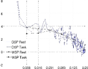
$\log_{2}\widehat{\Gamma}_{{\mathb{u}}_{s,k}}(f)$ $\log_{2}S^{d}_{{\mathb{u}}_{s,k}}(j,2)$		${\mathcal{D}}(h)$
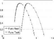
	(a)		(b)
	$\log_{2}f$ in Hz		Hölder exponent $h$

Figure 2: (a): Welch (blue curves) vs. Wavelet (black curves) spectra associated with a F-map (${\mathb{f}}_{18}$). Solid and dashed lines correspond to rest and task, respectively. (b): Corresponding multifractal spectra ${\mathcal{D}}(h)$.

5.1.3 Multifractal spectrum

For the same time series, MF spectra ${\mathcal{D}}(h)$, estimated using the WLMF tool described above, are depicted in Fig. 2(b). The decrease of self-similarity between rest and task is captured by a shift to the left of the position $\widehat{c}_{1}$ of the maximum of ${\cal D}(h)$: $\bigl{(}(\widehat{c}_{1})_{{\mathb{f}}_{18}}^{\rm R},(\widehat{c}_{1})_{{\mathb{f}}_{18}}^{\rm T}\bigr{)}\!=\!(0.75,0.5)$ It should also be noted that parameter $\widehat{c}_{1}$ systematically takes values that are close to those of the Hurst exponent. This is consistent with the theoretical modeling of scale-free property that establishes a clear connection between $c_{1}$ and $H$ and predicts $c_{1}\!\simeq\!H$ (cf. [73]). Therefore, in the following, $c_{1}$ will be referred to as the self-similarity parameter although this is a slight misnomer. Further, Fig. 2(b) confirms the presence of multifractality in fMRI data as strictly negative $c_{2}\!<\!0$ are almost always observed. Indeed, parameter $c_{2}$ quantifies the width of ${\cal D}(h)$ (as a curvature radius of ${\cal D}(h)$ around $\widehat{c}_{1}$): $\widehat{c}_{2}\!<\!0$. Multifractality is however not specific to a given brain state since we measured $\bigl{(}(\widehat{c}_{2})_{{\mathb{f}}_{18}}^{\rm R},(\widehat{c}_{2})_{{\mathb{f}}_{18}}^{\rm T}\bigr{)}\!=\!(-0.07,-0.06)$. In this example, multifractality, as measured by the width of the multifractal spectra, is decreased from rest to task. However, opposite fluctuations will be also observed amongst F-maps.

The sole two self-similarity and multifractality parameters $c_{1}$ and $c_{2}$ are therefore used from now on as sufficient and relevant descriptors of the scale-free properties of fMRI signals (superscript $\gamma$ is dropped for the sake of conciseness, while $\gamma$ has been systematically set to $\gamma=2$).

5.2 Group-level analysis

5.2.1 Group level scale-free properties

Let $c_{i,k}^{j,s}$ denote the $\widehat{c}_{1}$ and $\widehat{c}_{2}$ estimates (index $i=1\!\!:\!\!2$) for differents maps (index $k=1\!\!:\!\!K$), runs (index $j={\rm R,T}$ for Rest and Task, respectively) and for different subjects (index $s$). The map-dependent group-level values have been computed as $\mu_{i,k}^{j}\!=\!\sum_{s=1}^{S}\widehat{c}^{j,s}_{i,k}/S$ and sorted according to their labelling (F/A/U maps) given in Tab. 1. Then, global spatial averaging of the means $\mu_{i,k}^{j}$ has been performed so as to derive global F/A/U-average parameter estimates: $\bar{\mu}_{i,F}^{j}\!=\!\sum_{k\subset{\mathcal{F}}}\mu_{i,k}^{j}/{\mathrm{Card}}\left({\mathcal{F}}\right)\,$, $\bar{\mu}_{i,A}^{j}$ and $\bar{\mu}_{i,U}^{j}$ are defined equivalently. In the same spirit, group-level multifractal attributes $\bar{\mu}_{i,v_{\ell}}^{j}$ are derived for each functional network $v_{\ell}\in{\mathcal{N}}\!\!=\!\!\left\{\text{Att},\text{DMN},\text{Mot},\text{N-c},\text{Vis}\right\}$ such that $\bar{\mu}_{i,{\mathb{n}}_{\ell}}^{j}\!\!=\!\!\sum_{k\in{\mathb{n}}_{\ell}}\mu_{i,k}^{j}/{\mathrm{Card}}\left({\mathb{n}}_{\ell}\right)$, $\forall\ell=1:5$ and $j=({\rm R,T})$. We proceed in the same way for analyzing artifact types ${\mathb{t}}_{r}\in{\mathcal{T}}\!\!=\!\!\left\{\text{Ven},\text{WhM},\text{Mov},\text{Oth}\right\}$, and computing $\bar{\mu}_{i,{\mathb{t}}_{r}}^{j}$ for $r=1:4$.

As shown in Fig. 3[top], the group-averaged values of self-similarity $\mu_{1,k}^{j}$ lie approximately in the same range [.55, 1], indicating long memory, for all components (F/A/U-maps). An almost systematic decrease of self-similarity is observed in the task-related dataset ($\delta_{1,k}\!=\!\mu_{1,k}^{\rm T}-\mu_{1,k}^{\rm R}\!<\!0$), for $k\in{\mathcal{F}}\cup{\mathcal{A}}\cup{\mathcal{U}}$. This trend is therefore not specific to F-maps. Moreover, the average decrease computed over F-maps is about the same as the one estimated for A and U-maps ($\bar{\delta}_{1,F}\!=\!-0.125$, $\bar{\delta}_{1,A}\!=\!-0.11$ and $\bar{\delta}_{1,U}\!=\!-0.13$). Also, the averaged standard deviations ($\bar{\sigma}^{\rm R}_{1,F}$, $\bar{\sigma}^{\rm R}_{1,A}$ and $\bar{\sigma}^{\rm R}_{1,U}$) computed over the F/A/U-maps, are close to each other $(\bar{\sigma}^{\rm R}_{1,F/A/U}\approx 0.18)$ and systematically increase with the task-related activity ($\bar{\sigma}^{\rm T}_{1,F/A/U}\!>\!\bar{\sigma}^{\rm R}_{1,F/A/U}$).

Fig. 3[bottom] illustrates that the group-averaged values of $\mu_{2,k}^{\rm R,T}$ are almost all negative in the F/A/U-maps indicating multifractality in fMRI time series irrespective of the map type or brain state. Between rest to task-related situation minor changes in the A and U-maps are also observed since $\left|\delta_{2,k}\right|\!<\!0.03$ for $k\in{\mathcal{U}}\cup{\mathcal{A}}$ while we measured $\left|\delta_{2,k}\right|\!<\!0.08$ for $k\in{\mathcal{F}}$ ($\delta_{2,k}\!=\!\mu_{2,k}^{\rm T}-\mu_{2,k}^{\rm R}$). Hence, the level of multifractality does not change much between rest and task in irrelevant maps. In contrast, large changes in the multifractal parameters are observed in F-maps, while not systematically in the same direction. For instance, in cerebellum (${\mathb{f}}_{4}$), basal ganglia (${\mathb{f}}_{5}$), DMN (${\mathb{f}}_{7}$) and fronto-parietal network (${\mathb{f}}_{8}$) evoked activity induces a large increase of multifractality ($\delta_{2,k}\!<\!0$) while in the auditory and attentional systems (e.g. ${\mathb{f}}_{12}$ and ${\mathb{f}}_{24}$, respectively), which are supposed to be involved in the auditory detection task, the converse observation holds, i.e. $\delta_{2,k}\!>\!0$. Also, it is worth noticing that the averaged standard deviations computed over the A/U-maps increase when switching from rest to task ($\bar{\sigma}^{\rm R}_{2,A}\!=\!0.06<\bar{\sigma}^{\rm T}_{2,A}\!=\!0.09$ and $\bar{\sigma}^{\rm R}_{2,U}\!=\!0.05\!<\!\bar{\sigma}^{\rm T}_{2,U}\!=\!0.085$) while they remain at the same level in the F-maps: $\bar{\sigma}^{\rm R}_{2,F}\!\approx\!\bar{\sigma}^{\rm T}_{2,F}\!\approx\!0.08$.

$\mu_{1,k}^{j}$
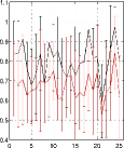
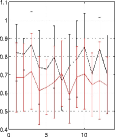
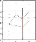
	F-maps	A-maps	U-maps
$\mu_{2,k}^{j}$
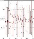
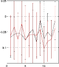
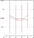
	$k\in{\mathcal{F}}$	$k\in{\mathcal{A}}$	$k\in{\mathcal{U}}$

Figure 3: From left to right: Group-averaged map-dependent MF parameters $\mu_{1,k}^{j}$ (top), $\mu_{2,k}^{j}$ (bottom) specific to F/A/U-maps defined in Tab. 1. Black and red curves code for $j={\rm R}$ (Rest) and $j={\rm T}$ (Task).

We computed the grand means of the self-similarity parameters $\bar{\mu}_{1,F/A/U}^{\rm R,T}$ over the F/A/U-maps, respectively, and draw the same conclusion at this macroscopic level, as demonstrated in Fig. 4(a)-(c): the decrease of self-similarity from rest to task is not specific to functional components and only slightly fluctuates between networks and artifact types. Moreover, we did not observe any significant modification of the grand means of multifractal parameter estimates $\bar{\mu}_{2,F/A/U}^{\rm R,T}$ between rest and task, as illustrated in Fig. 4(d). This motivated deeper investigations at the network and artifact levels, especially concerning the fluctuation of multifractality induced by task. Fig. 4(e) reveals that a major increase of multifractality ($\bar{\mu}_{2,{\mathb{n}}_{4}}^{\rm T}\!<\!\bar{\mu}_{2,{\mathb{n}}_{4}}^{\rm R}$) occurred only in the non-cortical regions while no major change appeared in the artifacts ($\bar{\mu}_{2,{\mathb{t}}_{r}}^{\rm T}\!\simeq\!\bar{\mu}_{2,{\mathb{t}}_{r}}^{\rm R},\forall r\!\in\!{\mathcal{T}}$) as shown in Fig. 4(f).

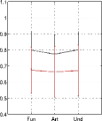
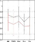
$\bar{\mu}_{1,F/A/U}^{j}$		$\bar{\mu}_{1,v_{\ell}}^{j}$		$\bar{\mu}_{1,w_{r}}^{j}$
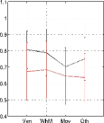
	(a)		(b)		(c)
	Averaged map type		Networks		artifacts
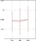
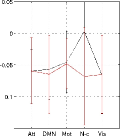
$\bar{\mu}_{2,F/A/U}^{j}$		$\bar{\mu}_{2,{\mathb{n}}_{\ell}}^{j}$		$\bar{\mu}_{2,{\mathb{t}}_{r}}^{j}$
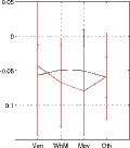
	(d)		(e)		(f)

Figure 4: Group-level MF parameters averaged over the F/A/U-maps $\bar{\mu}_{i,F/A/U}^{j}$ (Left), the functional networks $\bar{\mu}_{i,{\mathb{n}}_{\ell}}^{j}$ (Middle) and the artifact types $\bar{\mu}_{i,{\mathb{t}}_{r}}^{j}$ (Right). Black and red curves code for $j={\rm R}$ (Rest) and $j={\rm T}$ (Task).

5.2.2 One-sample statistical tests

To assess the statistical significance of the multifractal parameters for the rest and task-related datasets at the group-level, we used one-sided tests associated with the following null hypotheses $\forall k\in{\mathcal{F}}\cup{\mathcal{A}}\cup{\mathcal{U}}$:

$$\left.\begin{array}[]{ll}H_{0,j}^{(1,k)}:\mu_{1,k}^{j}&\leqslant 0.5,\quad\quad\text{(White noise or SRD)}\\ H_{0,j}^{(2,k)}:\mu_{2,k}^{j}&=0.,\quad\quad\text{(H-sssi process)}.\end{array}\right\}$$ (16)

We also conducted similar tests at the macroscopic level ($k\in{\mathcal{N}}\cup{\mathcal{T}}$) by replacing $\mu_{i,k}^{j}$ with $\bar{\mu}_{i,k}^{j}$ in the null hypotheses (16). Because there is no definite proof nor evidence that MF parameter estimates $\widehat{c}_{i,k}^{j,s}$ should be normally distributed across subjects, we investigated different statistics (Student-$t$, Wilcoxon’s signed rank (WSR) statistic). Indeed, other statistics may provide more sensitive results in presence of outliers. To account for multiple comparisons ($K$ tests performed simultaneously) and to ensure correct specificity control (control of false positives), the Bonferroni correction was applied.

Rejecting $H_{0,j}^{(1,k)}$ clearly amounts to localizing brain areas or components eliciting significant long memory or self-similarity. Rejecting $H_{0,j}^{(2,k)}$ enables to discriminate multifractality from self-similarity. Similar tests involving $\bar{\mu}_{i,F/A/U}^{j}$, $\bar{\mu}_{i,{\mathb{n}}_{\ell}}^{j}$ and $\bar{\mu}_{i,{\mathb{t}}_{r}}^{j}$ in the definition of null hypotheses (16) for $(i=1,2)$ were also performed.

corr. P-val.
	(a)	(b)
	Rest	Task
	$k\in{\mathcal{F}}$	$k\in{\mathcal{F}}$
corr. P-val.
	(c)	(d)
	$k\in{\mathcal{A}}$	$k\in{\mathcal{A}}$
corr. P-val.
	(e)	(f)
	$k\in{\mathcal{U}}$	$k\in{\mathcal{U}}$

Figure 5: Corrected p-values associated with one-sample Student-t (–,–) and WSR (-.,-.) tests performed for testing $H_{0,j}^{(1,\cdot)}$ (blue curves) and $H_{0,j}^{(2,\cdot)}$ (red curves) on the F- (top), A- (center) and U-maps (bottom), respectively, for $j={\rm R}$ (left) and $j={\rm T}$ (right). Significance level ($\alpha=.05$) is shown in - -.

Analysis of statistical significance of F-maps regarding $H_{0,R}^{(1),k}$ showed that most components (22/25) rejected this null hypothesis at rest using T-test and thus were significantly self-similar (see blue curves in Fig. 5(a)). The task effect then induced a loss of significance in the vast majority of components as shown in Fig. 5(b): only four maps (${\mathb{f}}_{10}$, ${\mathb{f}}_{14}$, ${\mathb{f}}_{18}$ and ${\mathb{f}}_{24}$) demonstrated a significant level of self-similarity using T-test in the task-related dataset. These maps are related to the motor, fronto-parietal and attentional (parieto-temporal junction and IPS/FEF) networks. Two out of them are lateralized in the left hemisphere. Statistical analysis of F-maps regarding $H_{0,R}^{(2),k}$ demonstrated that only six components (${\mathb{f}}_{15}$, ${\mathb{f}}_{17}$, ${\mathb{f}}_{18}$, ${\mathb{f}}_{21}$, ${\mathb{f}}_{23}$, ${\mathb{f}}_{24}$) rejected this null hypothesis at rest: see red curves in Fig. 5(a). The task-related modulation tends to reduce the number of significant F-maps: As depicted in Fig. 5(b), only 3 components survived the T-test (${\mathb{f}}_{10}$, ${\mathb{f}}_{15}$ and ${\mathb{f}}_{19}$) in the task-related dataset. Interestingly, ${\mathb{f}}_{10}$ and ${\mathb{f}}_{19}$ are likely to be involved in the auditory detection task and the motor response since they belong to the Motor and Attentional networks. Hence, a significant level of multifractality is observed during task in components that were monofractal at rest. Besides, the level of multifractality remains significant in the ventral occipital cortex (${\mathb{f}}_{15}$) irrespective of the brain state and that a few components in the visual (${\mathb{f}}_{17}$), fronto-parietal (${\mathb{f}}_{18}$), temporal (${\mathb{f}}_{21}$), prefrontal (${\mathb{f}}_{23}$) and attentional (${\mathb{f}}_{24}$) networks became monofractal under the task effect.

Statistical analysis of A and U-maps regarding $H_{0,j}^{(1),k}$ showed the same behavior when switching from rest to task, namely a strong decrease of the number of significant self-similar components (from 10 to 4 and 4 to 2 for A/U-maps, respectively): see blue curves in Fig. 5(c)-(d) and Fig. 5(e)-(f), respectively. Statistical analysis of A and U-maps regarding $H_{0,j}^{(2),k}$ also demonstrated a reduction of the number of multifractal components in A/U-maps. Two artifactual components (${\mathb{a}}_{10}$ and ${\mathb{a}}_{12}$) located in the white matter remained consistently multifractal in both datasets and one undefined component (${\mathb{u}}_{3}$) became significantly multifractal when switching from rest to task. In all cases, a loss of significance is observed using WSR tests (dash dotted curves) instead of T-tests (solid curves) indicating that there is no outlier in this group and thus that the Gaussian distribution hypothesis is tenable.

corr. P-val.
	(a)	(b)
	Rest	Task
corr. P-val.
	(c)	(d)
corr. P-val.
	(e)	(f)

Figure 6: Corrected p-values associated with one-sample Student-t (–,–) and WSR (-.,-.) tests performed for testing $\bar{H}_{0,j}^{(1,\cdot)}$ (blue curves) and $\bar{H}_{0,j}^{(2,\cdot)}$ (red curves) on the the averaged map types (top), networks (center) and artifact types (bottom), respectively for $j={\rm R}$ (left) and $j={\rm T}$ (right). Significance level ($\alpha=.05$) is shown in - -.

Then, we focused on the statistical analysis at different macroscopic scales, first by averaging all F/A and U-maps respectively so as to derive a mean behavior for F/A/U-maps. Finally, we looked at functional networks and artifact types in more details. Blue curves in Fig. 6(a)-(b) report such results for the rest and task-related datasets, respectively. We still observed a significant level of self-similarity in all averaged groups (blue curves) irrespective of the brain state: $\bar{H}_{0,j}^{(1,F/A/U)}$ is systematically rejected for $j=({\rm R,T})$. However, we still noticed a reduction of statistical significance induced by task irrespective of the map type. More interestingly, we found at this macroscopic level that all averaged maps were multifractal at rest whereas only the functional one remained multifractal during task: see red curves in Fig. 6(a)-(b). Further, statistical analysis of functional networks defined in Tab. 1 was conducted to understand which network drives this effect. When comparing p-values in Fig. 6(c)-(d) on functional networks, we observed that all remained significantly self-similar in both states, while the DMN is close to the significance level $\alpha\!=\!0.05$ during task (blue curves). Regarding multifractality, only the non-cortical regions appeared monofractral at rest and all networks kept a significant amount of multifractality during task. In contrast, this observation did not hold for artifacts: when looking at Fig. 6(e)-(f) in detail, the signal related to ventricles became monofractal during task.

5.2.3 2-way repeated measures ANOVA

In order to assess any significant change of self-similarity or multifractality between rest and task, we entered the subject-dependent parameter estimates $(\widehat{c}_{i,k}^{j,s})$ in several 2-way repeated measures ANOVAs involving two factors: brain state (two values: $j={\rm R,T}$) and map type (with varying number of values). These ANOVAs were conducted separately for assessing self-similarity ($i=1$) and multifractality ($i=2$) changes. First six ANOVAs (three for each parameter) were carried out by considering the F/A/U-maps as the second factor, respectively. This second factor thus took a number of values that depends on the set under study: ${\mathcal{F}}$, ${\mathcal{A}}$ or ${\mathcal{U}}$. Results are summarized in Tab. 2. Regarding the analysis of self-similarity ($\widehat{c}_{1,k}^{j,s}$ parameters), a significant brain state effect appeared in all F/A/U-maps, and a significant map effect in the F and A-sets. Significant interactions were found for the F and U-maps. This confirms that the level of self-similarity is not sufficient to disentangle functional networks from artifactual or undefined maps.
As regards ANOVAs based on $\widehat{c}_{2,k}^{j,s}$ parameters, a significant interaction for F-maps is found, thus indicating that the averaged change in multifractality between rest and task is significant for functional maps only. In summary, only F-maps exhibited significant interactions for both multifractal attributes.

Table 2: 2-way repeated measures ANOVA results based on the $\widehat{c}_{i,k}^{j,s}$ parameters for $i=\left\{1,2\right\}$, $j=({\rm R,T})$, $s=1:S$ and $k\in{\mathcal{F}}$ (top), $k\in{\mathcal{A}}$ (middle), $k\in{\mathcal{U}}$ (bottom).

Level	Param.	Source	F score	p-val.
F-maps	$\widehat{c}_{1,k}^{j,s}$	State	9.54	0.01
		Map	4.31	1e-09
		State $\times$ Map	1.76	0.02
F-maps	$\widehat{c}_{2,k}^{j,s}$	State	0.13	0.73
		Map	1.19	0.25
		State $\times$ Map	1.56	0.04
A-maps	$\widehat{c}_{1,k}^{j,s}$	State	5.73	0.03
		Map	2.4	0.008
		State $\times$ Map	1.32	0.21
A-maps	$\widehat{c}_{2,k}^{j,s}$	State	0.09	0.77
		Map	2.4	0.007
		State $\times$ Map	0.71	0.74
U-maps	$\widehat{c}_{1,k}^{j,s}$	State	5.39	0.04
		Map	2.91	0.06
		State $\times$ Map	3.16	0.04
U-maps	$\widehat{c}_{2,k}^{j,s}$	State	2.43e-05	0.99
		Map	0.68	0.57
		State $\times$ Map	0.63	0.6

Akin to the one-sample analyses above, we looked at a larger spatial scale, the functional network and artifact type levels and performed similar ANOVAs, corresponding results are reported in Tab. 3. While both functional networks and artifacts demonstrate a significant change in the self-similarity parameter between rest and task, only functional networks made the map-type effect significant. More importantly, the key feature for discriminating functional networks from artifacts relied on ANOVAs based on $\widehat{c}_{2,k}^{j,s}$ parameters. Indeed, a significant network effect and more importantly a significant interaction between rest and task are observed in functional networks.

Table 3: 2-way repeated measures ANOVA results based on the $\widehat{c}_{i,k}^{j,s}$ parameters for $i=\left\{1,2\right\}$, $j=({\rm R,T})$, $s=1:S$ and $k\in{\mathcal{N}}$ (top) and $k\in{\mathcal{T}}$ (bottom).

Level	Param.	Source	F score	p-val.
Networks	$\widehat{c}_{1,k}^{j,s}$	State	9.78	0.01
		Network	4.18	0.006
		State $\times$ Network	1.09	0.37
Networks	$\widehat{c}_{2,k}^{j,s}$	State	1.013	0.34
		Network	3.18	0.02
		State $\times$ Network	2.97	0.03
artifacts	$\widehat{c}_{1,k}^{j,s}$	State	4.85	0.05
		artifact	2.33	0.09
		State $\times$ artifact	1.16	0.34
artifacts	$\widehat{c}_{2,k}^{j,s}$	State	0.31	0.59
		artifact	1.03	0.39
		State $\times$ artifact	1.085	0.37

5.2.4 Two-sample statistical tests

To localize which maps are responsible for statistically significant ANOVA results, we finally performed two-sample T-tests in which we tested the following null hypotheses:

$$\left\{\begin{array}[]{ll}\widetilde{H}_{0}^{(1,k)}:\mu_{1,k}^{\rm R}=\mu_{1,k}^{\rm T},\;\forall k\in{\mathcal{F}}\cup{\mathcal{A}}\cup{\mathcal{U}}\\ \widetilde{H}_{0}^{(2,k)}:\mu_{2,k}^{\rm R}=\mu_{2,k}^{\rm T},\;\forall k\in{\mathcal{F}}\cup{\mathcal{A}}\cup{\mathcal{U}}.\end{array}\right.$$ (17)

We also conducted similar tests at the macroscopic level ($k\in{\mathcal{N}}\cup{\mathcal{T}}$) by replacing $\mu_{i,k}^{j}$ with $\bar{\mu}_{i,k}^{j}$ in the null hypotheses (17). The fluctuations in self-similarity being systematically in the same direction between rest and task, we performed one-sided tests as regards the $\mu_{1,k}^{j}$’s while two-sided tests were considered for the $\mu_{2,k}^{j}$’s: task-related positive and negative fluctuations of $\mu_{2,k}^{j}$ were actually observed in Subsection 5.2.1. Fig. 7(a)-(b) shows the uncorrected p-values for the F-maps and networks, respectively. We rejected $\widetilde{H}_{0}^{(1,k)}$ for $\left({\mathb{f}}_{3},{\mathb{f}}_{4},{\mathb{f}}_{11},{\mathb{f}}_{18},{\mathb{f}}_{25}\right)$ at a significance level set to $\alpha_{1}\!=\!0.01$ and $\widetilde{H}_{0}^{(2,k)}$ for $\left({\mathb{f}}_{4},{\mathb{f}}_{7},{\mathb{f}}_{18}\right)$ at $\alpha_{2}\!=\!0.05$. These components clearly explain significant results reported in Tab. 2 about the changes in self-similarity and multifractality that occurred in F-maps. Interestingly, among the latter, the null hypothesis was rejected because of a large increase of multifractality in $({\mathb{f}}_{4},{\mathb{f}}_{7})$. In contrast, a decrease of multifractality was responsible for the rejection of $\widetilde{H}_{0}^{(2,k)}$ in ${\mathb{f}}_{18}$. When setting $\alpha_{2}\!=\!\alpha_{1}\!=\!0.01$, only ${\mathb{f}}_{18}$ survived this threshold and thus remained the single functional component for which a significant difference of self-similarity and multifractality was found between rest and task. This component clearly drove the significant interaction reported in Tab. 2 for the change in multifractality in F-maps. Fig. 7(b) also showed that the state effect reported in Tab. 3 on $(\widehat{c}_{1,k}^{j,s})$ at the network level was driven by the attentional, motor and visual systems. Last, the significant interaction reported in Tab. 3 on $(\widehat{c}_{2,k}^{j,s})$ is explained by the non-cortical regions as shown in Fig. 7(b).

Fig. 7(c)-(d) shows the localization of the state effects reported in Tabs. 2-3 for the changes in self-similarity that occurred in artifacts at the local and global levels. No A-map enabled to reject $\widetilde{H}_{0}^{(1,k)}$ at the $\alpha_{1}$ significance level but a majority of A-maps $\left({\mathb{a}}_{1:4},{\mathb{a}}_{6},{\mathb{a}}_{8},{\mathb{a}}_{10},{\mathb{a}}_{12}\right)$ contributed to the significant state effect observed in Tab. 2. At the global artifact level, the ventricles appear as the main source of the significant state effect reported in Tab.3 for the change in self-similarity. Also, no significant difference in multifractality was reported for artifacts whatever the observation level (A-maps or averaged artifacts). Similarly, Fig. 7(e) enables us to show that ${\mathb{u}}_{2}$ and ${\mathb{u}}_{4}$ were the main sources of the significant state effect and interactions reported in Tab. 2 for the change in self-similarity. At the macroscopic level, we finally observed in Fig. 7(f) that only the grand mean of functional maps leads to a significant modulation of self-similarity between rest and task at level $\alpha_{1}$.

unc. P-val.
	(a)	(b)
	F-maps	Networks
	$k\in{\mathcal{F}}$
unc. P-val.
	(c)	(d)
	A-maps	artifacts
	$k\in{\mathcal{A}}$
unc. P-val.
	(e)	(f)
	U-maps	Averaged map type
	$k\in{\mathcal{U}}$

Figure 7: Uncorrected p-values associated with two-samples Student-t test performed for testing $\widetilde{H}_{0}^{(1,\cdot)}$ (blue curves) and $\widetilde{H}_{0}^{(2,\cdot)}$ (red curves) on the the F/A/U-maps (left) and networks, artifacts and map types (right), respectively. Significance levels ($\alpha_{1}=.01$ and $\alpha_{2}=.05$) are shown in - - and - -, respectively.

6 Discussion

6.1 Results interpretation

This study analyzed in depth the scale-free properties of fMRI signals, using multifractal methodologies, and their modulations during rest and task both in functional networks and artifactual regions. The underlying goal was to finely characterize which properties are specific to functional networks and which modulation can be expected for these networks from task-related activity. Previous attempts in the literature [28, 46, 40] focused on functional networks without comparing results with the behavior of artifacts. The main reason comes from the fact that seed region analyses were only conducted in such studies. Hence, no comparison with vascular or ventricles-related signals was undertaken.

Our results confirmed that fMRI signals are stationary and self-similar but not specifically in functional networks. Also we showed that the amount of self-similarity significantly varies between rest and task not only in functional networks involved in our auditory detection task with a motor response (Attentional, Motor) but also quite surprisingly in the visual system and in some artifacts (ventricles) and undefined maps. This observation led us to investigate the scale-free structure of fMRI signals using richer models, namely multifractal processes, to which the WLMF toolbox is dedicated. Our statistical results demonstrate first that fMRI signals are multifractal, second that interactions between brain state and maps only occurred in F-maps and functional networks and third, that specific F-maps such as in non-cortical regions demonstrated a statistically significant fluctuation between rest and task. This result shows that the concept of multifractality permits to disentangle functional components from artifactual ones, in a robust and significant manner.

However, in contrast to self-similarity that systematically decreases with evoked activity, multifractality decreases in cortical (${\mathb{f}}_{18}$) but increases in non-cortical (${\mathb{f}}_{4},{\mathb{f}}_{7}$). Thus, task-related activity has no systematic impact with respect to increase/decrease of multifractality. Interestingly, we found a statistically non-significant trend towards a decrease of multifractality in regions primarily involved in the task (${\mathb{f}}_{12}$, ${\mathb{f}}_{24}$, ${\mathb{f}}_{25}$). However, the group size of this study remains small (12 subjects only) to achieve significant results, mainly because of the between-subject variability and of the difficulty in estimating $\widehat{c}_{2,k}^{j,s}$ parameters on short time series.

Further investigations beyond the scope of this paper are necessary to find out any general trend on the direction change of multifractality with evoked-activity by cross-correlating multifractal parameters with task-related activity (e.g. group-level Z-scores) and task performance. However, to derive reliable results for multifractality, a larger group of individuals will be considered and a larger number of scans will be acquired while maintaining the same scanning time: To this end, accelerated SENSE imaging will be used together with recent reconstruction algorithms so as to improve temporal resolution [21].

6.2 Monofractal scale-free EEG microstate sequences vs multifractal dynamics for RSN

The results obtained in this contribution shows multifractal temporal dynamics in fMRI signals and thus naturally lead to question the potential origins and generative mechanisms for this departure from the more traditional longe range correlation modeling of scale invariance. A natural track to inspect consists of that of the relations between hemodynamic (fMRI) and electrical (EEG) signatures for brain activity at rest. This question has been intensively studied over the last decade [45, 53, 12, 67, 56, 75], first by measuring cross correlations between fMRI data at rest and EEG-informed regressors derived from the convolution of the EEG power signal in five well-identified frequency bands ($\delta\in(1,4)$ Hz, $\theta\in(4,7)$ Hz, $\alpha\in(8,12)$ Hz, $\beta\in(13,30)$ Hz and $\gamma>30$ Hz) with the canonical HRF. This approach revealed the negative correlation of $\alpha$-band activity with the attentional network and the positive correlation with $\beta_{2}$-band with the default mode network (precuneus and posterior cingulate cortex) [45]. Also, [53] showed that functional resting state networks have different EEG signatures which are not specific to a given frequency band but are rather spread over several oscillations regimes (e.g., correlation between $\alpha$ and $\beta$ power in specific RSN), a consequence of the so-called oscillation hierarchy [18] and the of phase-amplitude cross-frequency coupling [41]. However, none of these works enable to explain the low frequency fluctuations ($<0.1$ Hz) or scale-free dynamics of the fMRI signal at rest, because this phenomenon is much more widespread than oscillations.

Scale-free dynamics of brain electrical activity at rest has recently been studied [67] but not directly on raw data. Instead, EEG microscates that correspond to short periods (100 ms) during which the EEG scalp topography remains quasi-stable, have been first segmented. Remarkably, it has been shown that only four different EEG microstate patterns are necessary to describe the ongoing electrical brain activity at rest [12] and that these four microscates correlate with well-known RSNs, which were classically identified from fMRI dataset alone using group-level ICA. This demonstrated that the EEG microstate with rapid fluctuations might be considered as the electrophysiological signature of intrinsic functional connectivity patterns. The investigation of scale-free dynamics was thus performed on the EEG microstate sequence to understand how fast the microscates are changing and what kind of correlation structure (short or long range) they bring [67].

The recent finding that EEG microscate sequences reveal purely monofractal dynamics [67], irrespective of the data filtering, may lead to conclude that the same monofractal behaviour in the fMRI signature of RSN (strongly correlate with these microstates) should be expected, if one assumes a linear and time invariant HRF model for the neurovascular coupling. However, the results obtained in the present contribution can be considered not only as evidence in favor of multifractality in fMRI data, but also as evidence that this multifractal effect is discriminant of cortical versus non cortical regions and characteristic of functional network with respect to modulation under task.

Several factors may explain this apparent discrepancy. First, an accurate comparison of both sets of result would require a precise match of the range of scales (or frequencies) within which scale invariance is analyzed and corresponding parameters measured. Here, the selected range of frequencies corresponds to ([.008, .063]Hz), while the monofractal behavior of EEG microstate sequences was exhibited on a distinct frequency range ie. ([.063, 3.9]Hz) in [67]. Comparison of scaling properties requires that the same frequency range is selected but this constraint is clearly not tenable across modalities like EEG and fMRI given the fMRI sampling rate.

Second, it is indeed very unlikely that a linear and time invariant filtering may create multifractality in fMRI starting from a monofractal electrophysiological signal in EEG. The general issue of the relations between (linear and non linear) filtering and multifractality were barely studied theoretically so far but interestingly, [3] has shown that simple nonlinear filter can turn mono- into multifractality. Hence, another putative origin for the apparent contradiction between our findings and those in [67] lies in refined descriptions of HRF model by nonlinear dynamical systems (e.g., Balloon model) [17, 16]. Of course, linear and stationary approximations like the canonical HRF model [38] or nonparametric alternatives [72, 20] have been validated but only on evoked activity and considering inter-stimulus intervals larger than 3 s. For shorter ISIs, nonlinear hemodynamics has turned out to be a valid property [48]. In this context, habituation or repetition supression effects may occur and induce a sublinear hemodynamic response, which would modify scaling properties [32, 26]. Hence, by modelling the sequence of EEG transient brain states as a series of short time epochs, this could induce nonlinearities in the hemodynamic system that could explain the switch from purely fractal EEG microstates to multifractal signatures in the corresponding RSNs.

Third, instead of segregating EEG microstates in multiple groups based upon the maximal spatial dissimilarity between groups [12, 56], a more recent analysis of joint EEG/fMRI resting state data has revealed a larger number (thirteen) of EEG microstates that show temporal independence from each other [75]. In this latter work, all resting state networks including visual, motor, auditory, attention, saliency and default mode networks were characterized by a specific electrophysiological signature involving several EEG microstates. This clearly indicates that the original analysis of scale-free dynamics for EEG microscates done in [67] should be revisited on this larger number of metastable states to disentangle whether multifractality in this larger set of microstates has been discarded due to averaging effects. It is actually clear that the sequence mixing thirteen different microstates may generate richer singularities (abrupt changes between microstates) than the ones relying on four microstates only. Fourth, the temporal signatures of EEG microstates found in [67, 56] are correlated in time since the spatial similarity was the key factor to identify them. As a consequence, the microstate sequences is correlated too and might loose some singularities that could be found out in the microstate sequences generated by [75]. Finally, the presence of multifractality in resting state (and task-related) MEG data has been evidenced in the sensor space in [78]. These findings open new research avenues: For instance, it is natural to explore whether the observed multifractal properties can be related multiplicative cascade processes, that is to one one of the only practical mechanism known to generate multifractal dynamics, or to investigate whether this cascade takes place at meso or macroscopic scales, as well as to figure out how brain networks could implement such cascade mechanisms. This topic is beyond the scope of the present contribution, however the log-normal statistics of neuronal firing rate could provide us with a first clue to uncover any generative process underlying multifractal dynamics.

6.3 Stationarity vs non-stationarity of the RSN dynamics

Recent results in resting state fMRI reveal temporally independent functional modes of spontaneous brain activity [64] and postulate the presence of temporally non-stationary modes in part of the default mode network by resorting to high temporal resolution fMRI. While stationarity receives a unique and clear definition, non stationarity can correspond to a bunch of different situations; for example, non-stationarity might (i) refer to an apparent change over time in the correlation between two regions or (ii) refer to changes in the mean and/or variance in the time course of a functional network.

The wavelet based analysis of scaling proposed here already addresses a number of such situations. The fact that the estimated Hurst coefficient of fMRI time series remains consistently below 1 indicates that fMRI signals at hand here are better modeled as a stationary step process $Y$ rather than as a non stationary random walk $X$. Further, wavelet analysis are known to bring robustness against various forms of non stationarities, such as smooth trends superimposed to data, to mean or variance modulation (cf (ii)). The multifractal analysis performed here is thus not impaired by such form of non stationarities. This leaves open issues such as the presence of oscillations superimposed to scaling. Given that time series are very short, the use of formal stationarity test will lack power and are not likely to reject stationarity. Further, in all the analysis conducted in the present work, no evidence of non-stationarity in the fMRI time series at hand were evidenced. This is in agreement with what has been reported in [40] in an fMRI ROI-based analysis. Finally, previous attempts to scale-free analysis of densely sampled fMRI datasets in time (using the EVI sequence [57] already confirmed the validity of a the stationarity assumption; see [25].

7 Conclusion

We uncovered multifractal scale-free dynamics of fMRI time series over four octaves (15s.-125s.) both in functional networks and in artifacts. We then disentangled functional components from artifactual ones in a robust and significant manner by demonstrating that only the former gave rise to significant modulations of the multifractal attributes between rest and task-related activity. Variability in human performance scores also generally exhibits power law distributions, whose strength (or exponent) is often modulated across conditions and tasks [43]. This paves the way towards future works devoted to investigating the extent to which behavioral properties are correlated with the change of scale-free dynamics in neuroimaging time series (MEG, fMRI) acquired during multisensory learning [61].

8 Acknowledgements

The authors thank the French National Research Agency (ANR) for its financial support to the SCHUBERT (ANR-09-JCJC-0071) young researcher project (2009-13). The authors are also grateful to the anonymous reviewers and the associate editor, Dr. BJ He, for their remarks and criticisms that helped us to improve the manuscript and enlarge the readership. Finally, we would like to warmly thank Dr. V. van Wassenhove for her careful rereading and constructive comments.

References

- Abry et al. [2002] P. Abry, R. Baraniuk, P. Flandrin, R. Riedi, D. Veitch, Multiscale network traffic analysis, modeling, and inference using wavelets, multifractals, and cascades, IEEE Signal Processing Magazine 3 (2002) 28–46.
- Abry et al. [1995] P. Abry, P. Gonçalvès, P. Flandrin, Wavelets, spectrum estimation and processes, Wavelets, spectrum estimation and processes, Springer-Verlag, New York, 1995. Wavelets and Statistics, Lecture Notes in Statistics.
- Abry et al. [2012] P. Abry, S. Jaffard, H. Wendt, Irregularities and scaling in signal and image processing: Multifractal analysis, in: M. Frame (Ed.), Benoit Mandelbrot: A Life in Many Dimensions, To Appear, Yale University, 2012.
- Abry et al. [1998] P. Abry, D. Veitch, P. Flandrin, Long-range dependence: revisiting aggregation with wavelets, Journal of Time Series Analysis 19 (1998) 253–266.
- Achard et al. [2006] S. Achard, R. Salvador, B. Whitcher, J. Suckling, E. Bullmore, A resilient, low-frequency, small-world human brain functional network with highly connected association cortical hubs., The Journal of neuroscience 26 (2006) 63–72.
- Arneodo et al. [2002] A. Arneodo, B. Audit, N. Decoster, J.F. Muzy, C. Vaillant, Wavelet-based multifractal formalism: applications to dna sequences, satellite images of the cloud structure and stock market data, The Science of Disasters; A. Bunde, J. Kropp, H.J. Schellnhuber, Eds. (Springer) (2002) 27–102.
- Bacry et al. [2001] E. Bacry, J. Delour, J. Muzy, Multifractal random walk, Phys. Rev. E 64 (2001) 026103.
- Bak and Paczuski [1995] P. Bak, M. Paczuski, Complexity, contingency, and criticality., Proceedings of the National Academy of Sciences of the United States of America 92 (1995) 6689–96.
- Barral and Mandelbrot [2002] J. Barral, B. Mandelbrot, Multifractal products of cylindrical pulses, Probability Theory and Related Fields 124 (2002) 409–430.
- Beckmann and Smith [2004] C. Beckmann, S. Smith, Probabilistic independent component analysis for functional magnetic resonance imaging, IEEE Transactions on Medical Imaging 23 (2004) 137–152.
- Biswal et al. [1995] B. Biswal, F. Zerrin Yetkin, V. Haughton, J. Hyde, Functional connectivity in the motor cortex of resting human brain using echo-planar MRI, Magnetic Resonance in Medicine 34 (1995).
- Britz et al. [2010] J. Britz, D. Van De Ville, C.M. Michel, BOLD correlates of EEG topography reveal rapid resting-state network dynamics., Neuroimage 52 (2010) 1162–70.
- Bullmore et al. [2001] E. Bullmore, C. Long, J. Suckling, J. Fadili, G. Calvert, F. Zelaya, T. Carpenter, M. Brammer, Colored noise and computational inference in neurophysiological (fMRI) time series analysis: resampling methods in time and wavelet domains, Human Brain Mapping 12 (2001) 61–78.
- Bullmore and Sporns [2009] E. Bullmore, O. Sporns, Complex brain networks: graph theoretical analysis of structural and functional systems., Nature reviews. Neuroscience 10 (2009) 186–98.
- Bullock et al. [2003] T. Bullock, M. Mcclune, J. Enright, Are the electroencephalograms mainly rhythmic? Assessment of periodicity in wide-band time series, Neuroscience 121 (2003) 233–252.
- Buxton et al. [2004] R.B. Buxton, K.U. g, D.J. Dubowitz, T.T. Liu, Modeling the hemodynamic response to brain activation, Neuroimage 23, Supplement 1 (2004) S220–S233.
- Buxton et al. [1998] R.B. Buxton, E.C. Wong, F.L. R., Dynamics of blood flow and oxygenation changes during brain activation: the balloon model, Magnetic Resonance in Medicine 39 (1998) 855–864.
- Buzsáki [2006] G. Buzsáki, Rhythms of the brain, Oxford university Press, New York, USA, 2006.
- Calhoun et al. [2001] V.D. Calhoun, T. Adali, G.D. Pearlson, J.J. Pekar, A method for making group inferences from functional MRI data using independent component analysis., Hum Brain Mapp 14 (2001) 140–151.
- Chaari et al. [2011a] L. Chaari, F. Forbes, T. Vincent, M. Dojat, P. Ciuciu, Variational solution to the joint detection estimation of brain activity in fMRI, in: 14thProceedings MICCAI’11, LNCS 6892 (Part II), Springer Verlag Berlin Heidelberg, Toronto, Canada, 2011a, pp. 260–268.
- Chaari et al. [2011b] L. Chaari, J.C. Pesquet, A. Benazza-Benyahia, P. Ciuciu, A wavelet-based regularized reconstruction algorithm for SENSE parallel MRI with applications to neuroimaging, Medical Image Analysis 15 (2011b) 185–201.
- Chainais et al. [2005] P. Chainais, R. Riedi, P. Abry, On non scale invariant infinitely divisible cascades, IEEE Trans. Info. Theory 51 (2005).
- Chialvo [2004] D.R. Chialvo, Critical brain networks, Physica A 340 (2004) 756–765.
- Chialvo [2010] D.R. Chialvo, Emergent complex neural dynamics, Nature Physics 6 (2010) 744–750.
- Ciuciu et al. [2008] P. Ciuciu, P. Abry, C. Rabrait, H. Wendt, Log Wavelet Leaders Cumulant Based Multifractal Analysis of EVI fMRI Time Series: Evidence of Scaling in Ongoing and Evoked Brain Activity, IEEE Journal of Selected Topics in Signal Processing 2 (2008) 929–943.
- Ciuciu et al. [2009] P. Ciuciu, S. Sockeel, T. Vincent, J. Idier, Modelling the neurovascular habituation effect on fMRI time series, in: Proc. of the 34th IEEEProceedings of the International Conference on Acoustic, Speech and Signal Processing, Taipei, Taiwan, pp. 433–436.
- Cole et al. [2010] D.M. Cole, S.M. Smith, C.F. Beckmann, Advances and pitfalls in the analysis and interpretation of resting-state FMRI data., Frontiers in systems neuroscience 4 (2010) 8.
- Cordes et al. [2001] D. Cordes, V. Haughton, K. Arfanakis, J. Carew, P. Turski, C. Moritz, M. Quigley, M. Meyerand, Frequencies contributing to functional connectivity in the cerebral cortex in ”resting-state” data., AJNR Am. J. Neuroradiol. 22 (2001) 1326–33.
- Dale [1999] A.M. Dale, Optimal experimental design for event-related fMRI, Human Brain Mapping 8 (1999) 109–114.
- Damoiseaux et al. [2006] J.S. Damoiseaux, S.A.R.B. Rombouts, F. Barkhof, P. Scheltens, C.J. Stam, S.M. Smith, C.F. Beckmann, Consistent resting-state networks across healthy subjects., Proc Natl Acad Sci U S A 103 (2006) 13848–13853.
- Daubechies et al. [2009] I. Daubechies, E. Roussos, S. Takerkart, M. Benharrosh, C. Golden, K. D’Ardenne, W. Richter, J.D. Cohen, J. Haxby, Independent component analysis for brain fmri does not select for independence., Proc Natl Acad Sci U S A 106 (2009) 10415–10422.
- Dehaene-Lambertz et al. [2006] G. Dehaene-Lambertz, S. Dehaene, J.L. Anton, A. Campagne, P. Ciuciu, G.P. Dehaene, I. Denghien, A. Jobert, D. Le Bihan, M. Sigman, C. Pallier, J.B. Poline, Functional segregation of cortical language areas by sentence repetition, Human Brain Mapping 27 (2006) 360–371.
- Eguiluz et al. [2005] V.M. Eguiluz, D.R. Chialvo, G.A. Cecchi, M. Baliki, A.V. Apkarian, Scale-Free Brain Functional Networks, Physical Review Letters 94 (2005) 1–4.
- Eke et al. [2002] A. Eke, P. Herman, L. Kocsis, L.R. Kozak, Fractal characterization of complexity in temporal physiological signals, Physiological Measurement 23 (2002) R1–R38.
- Fadili and Bullmore [2002] J. Fadili, E. Bullmore, Wavelet-generalized least squares: A new BLU estimator of linear regression models with 1/f errors, Neuroimage 15 (2002) 217–232.
- Fox et al. [2007] M.D. Fox, A.Z. Snyder, J.L. Vincent, M.E. Raichle, Intrinsic fluctuations within cortical systems account for intertrial variability in human evoked brain responses, Proceedings of the National Academy of Sciences of the United States of America 56 (2007) 171–84.
- Friston et al. [1995] K. Friston, A.P. Holmes, K. Worlsey, J.B. Poline, C. Frith, R. Frackowiak, Statistical parametric maps in functional neuroimaging: a general linear approach, Human Brain Mapping 2 (1995) 189–210.
- Glover [1999] G.H. Glover, Deconvolution of impulse response in event-related BOLD fMRI, Neuroimage 9 (1999) 416–429.
- Greicius et al. [2003] M. Greicius, B. Krasnow, A. Reiss, V. Menon, Functional connectivity in the resting brain: a network analysis of the default mode hypothesis, Proceedings of the National Academy of Sciences 100 (2003) 253–258.
- He [2011] B. He, Scale-Free Properties of the Functional Magnetic Resonance Imaging Signal during Rest and Task, Journal of Neuroscience 31 (2011) 13786–13795.
- He et al. [2010] B. He, J. Zempel, A. Snyder, M. Raichle, The Temporal Structures and Functional Significance of Scale-free Brain Activity, Neuron 66 (2010) 353–369.
- Hebiri and van de Geer [2011] M. Hebiri, S. van de Geer, The smooth-lasso and other ℓ1+ ℓ2-penalized methods, Electronic Journal of Statistics 5 (2011) 1184–1226.
- Holden et al. [2011] J.G. Holden, I. Choi, P.G. Amazeen, G. Van Orden, Fractal 1/f dynamics suggest entanglement of measurement and human performance., Journal of experimental psychology. Human perception and performance 37 (2011) 935–48.
- Kiviniemi et al. [2003] V. Kiviniemi, J. Kantola, J. Jauhiainen, A. Hyvärinen, O. Tervonen, Independent component analysis of nondeterministic fMRI signal sources, Neuroimage 19 (2003) 253–260.
- Laufs et al. [2003] H. Laufs, K. Krakow, P. Sterzer, E. Eger, a. Beyerle, a. Salek-Haddadi, a. Kleinschmidt, Electroencephalographic signatures of attentional and cognitive default modes in spontaneous brain activity fluctuations at rest., Proceedings of the National Academy of Sciences of the United States of America 100 (2003) 11053–8.
- Leopold et al. [2003] D. Leopold, Y. Murayama, N. Logothetis, Very slow activity fluctuations in monkey visual cortex: implications for functional brain imaging., Cerebral Cortex 13 (2003) 422–33.
- Linkenkaer-Hansen et al. [2001] K. Linkenkaer-Hansen, V. Nikouline, J. Palva, R. Ilmoniemi, Long-range temporal correlations and scaling behavior in human brain oscillations, The Journal of neuroscience : the official journal of the Society for Neuroscience 21 (2001) 1370–7.
- Liu and Gao [2000] H.L. Liu, J.H. Gao, An investigation of the impulse functions for the nonlinear BOLD response in functional MRI, Magnetic Resonance Imaging 18 (2000) 11053–11058.
- Makni et al. [2005] S. Makni, P. Ciuciu, J. Idier, J.B. Poline, Joint detection-estimation of brain activity in functional MRI: a multichannel deconvolution solution, IEEE Transactions on Signal Processing 53 (2005) 3488–3502.
- Makni et al. [2008] S. Makni, J. Idier, T. Vincent, B. Thirion, G. Dehaene-Lambertz, P. Ciuciu, A fully Bayesian approach to the parcel-based detection-estimation of brain activity in fMRI, Neuroimage 41 (2008) 941–969.
- Mallat [2009] S. Mallat, A Wavelet Tour of Signal Processing: The Sparse Way, Academic Press, Burlington, MA, 2009.
- Mandelbrot and van Ness [1968] B. Mandelbrot, J. van Ness, Fractional Brownian motion, fractional noises and applications, SIAM Reviews 10 (1968) 422–437.
- Mantini et al. [2007] D. Mantini, M.G. Perrucci, C. Del Gratta, G.L. Romani, M. Corbetta, Electrophysiological signatures of resting state networks in the human brain., Proceedings of the National Academy of Sciences of the United States of America 104 (2007) 13170–5.
- Maxim et al. [2005] V. Maxim, L. Sendur, J. Fadili, J. Suckling, R. Gould, R. Howard, E. Bullmore, Fractional Gaussian noise, functional MRI and Alzheimer’s disease., Neuroimage 25 (2005) 141–158.
- McKeown et al. [1998] M. McKeown, S. Makeig, G. Brown, T. Jung, S. Kindermann, A. Bell, T. Sejnowski, Analysis of fMRI data by blind separation into independent spatial components, Hum Brain Map 6 (1998) 160–188.
- Musso et al. [2010] F. Musso, J. Brinkmeyer, a. Mobascher, T. Warbrick, G. Winterer, Spontaneous brain activity and EEG microstates. A novel EEG/fMRI analysis approach to explore resting-state networks., Neuroimage 52 (2010) 1149–61.
- Rabrait et al. [2008] C. Rabrait, P. Ciuciu, A. Ribès, C. Poupon, P. Leroux, V. Lebon, G. Dehaene-Lambertz, D. Le Bihan, F. Lethimonnier, High temporal resolution functional MRI using parallel echo volume imaging, Journal of Magnetic Resonance Imaging 27 (2008) 744–753.
- Rosen et al. [1998] B.R. Rosen, R.L. Buckner, A.M. Dale, Event-related functional MRI: past, present and future., Proceedings of the National Academy of Sciences of the United States of America 95 (1998) 773–780.
- Sadaghiani et al. [2009] S. Sadaghiani, G. Hesselmann, A. Kleinschmidt, Distributed and antagonistic contributions of ongoing activity fluctuations to auditory stimulus detection, Journal of Neuroscience 29 (2009) 13410–13417.
- Samorodnitsky and Taqqu [1994] G. Samorodnitsky, M. Taqqu, Stable non-Gaussian random processes, Chapman and Hall, New York, 1994.
- Seitz et al. [2007] A. Seitz, R. Kim, V. van Wassenhove, L. Shams, Simultaneous and independent acquisition of multisensory and unisensory associations., Perception 36 (2007) 1445–1453.
- Shimizu et al. [2004] Y. Shimizu, M. Barth, C. Windischberger, E. Moser, S. Thurner, Wavelet-based multifractal analysis of fMRI time series., Neuroimage 22 (2004) 1195–1202.
- Smith et al. [2009] S. Smith, P. Fox, K. Miller, D. Glahn, P. Fox, C. Mackay, N. Filippini, K. Watkins, R. Toro, A. Laird, et al., Correspondence of the brain’s functional architecture during activation and rest, PNAS 106 (2009) 13040.
- Smith et al. [2012] S.M. Smith, K.L. Miller, S. Moeller, J. Xu, E.J. Auerbach, M.W. Woolrich, C.F. Beckmann, M. Jenkinson, J. Andersson, M.F. Glasser, D.C. Van Essen, D.a. Feinberg, E.S. Yacoub, K. Ugurbil, Temporally-independent functional modes of spontaneous brain activity., Proceedings of the National Academy of Sciences of the United States of America 109 (2012) 3131–6.
- Stam and de Bruin [2004] C.J. Stam, E.A. de Bruin, Scale-free dynamics of global functional connectivity in the human brain., Human Brain Mapping 22 (2004) 97–109.
- Thurner et al. [2003] S. Thurner, E. Windischberger, C. Moser, P. Walla, M. Barth, Scaling laws and persistence in human brain activity, Physica A 326 (2003) 511–521.
- Van de Ville et al. [2010] D. Van de Ville, J. Britz, C.M. Michel, EEG microstate sequences in healthy humans at rest reveal scale-free dynamics., Proceedings of the National Academy of Sciences of the United States of America 107 (2010) 18179–84.
- Varoquaux et al. [2011] G. Varoquaux, A. Gramfort, F. Pedregosa, V. Michel, B. Thirion, Multi-subject dictionary learning to segment an atlas of brain spontaneous activity, in: Information Processing in Medical Imaging, Springer, pp. 562–573.
- Varoquaux et al. [2010a] G. Varoquaux, M. Keller, J. Poline, P. Ciuciu, B. Thirion, ICA-based sparse features recovery from fMRI datasets, in: Proc. of the 7th IEEE International Symposium on Biomedical Imaging, Rotterdam, The Netherlands, pp. 1177–1180.
- Varoquaux et al. [2010b] G. Varoquaux, S. Sadaghiani, P. Pinel, A. Kleinschmidt, J.B. Poline, B. Thirion, A group model for stable multi-subject ICA on fMRI datasets, Neuroimage 51 (2010b) 288–299.
- Veitch and Abry [2001] D. Veitch, P. Abry, A statistical test for the time constancy of scaling exponents, IEEE Trans. on Sig. Proc. 49 (2001) 2325–2334.
- Vincent et al. [2010] T. Vincent, L. Risser, P. Ciuciu, Spatially adaptive mixture modeling for analysis of within-subject fMRI time series, IEEE Transactions on Medical Imaging 29 (2010) 1059–1074.
- Wendt et al. [2007] H. Wendt, P. Abry, S. Jaffard, Bootstrap for empirical multifractal analysis, IEEE Signal Processing Mag. 24 (2007) 38–48.
- Wink et al. [2008] A.M. Wink, E. Bullmore, A. Barnes, F. Bernard, J. Suckling, Monofractal and multifractal dynamics of low frequency endogenous brain oscillations in functional MRI., Human Brain Mapping 29 (2008) 791–801.
- Yuan et al. [2012] H. Yuan, V. Zotev, R. Phillips, W.C. Drevets, J. Bodurka, Spatiotemporal dynamics of the brain at rest - Exploring EEG microstates as electrophysiological signatures of BOLD resting state networks., NeuroImage (2012).
- Zarahn et al. [1997] E. Zarahn, G.K. Aguirre, M. D’Esposito, Empirical analysis of BOLD fMRI statistics. I. Spatially unsmoothed data collected under null-hypothesis conditions, Neuroimage 5 (1997) 179–197.
- Zemanová et al. [2006] L. Zemanová, C. Zhou, J. Kurths, Structural and functional clusters of complex brain networks, Physica D: Nonlinear Phenomena 224 (2006) 202–212.
- Zilber et al. [2012] N. Zilber, P. Ciuciu, P. Abry, V. van Wassenhove, Modulation of scale-free properties of brain activity in MEG, in: Proc. of the 9th IEEE International Symposium on Biomedical Imaging, Barcelona, Spain, pp. 1531–1534.