Scaling of Temperature Dependence of Charge Mobility
in Molecular Holstein Chains

Abstract

The temperature dependence of a charge mobility in a model DNA based on Holstein Hamiltonian is calculated for 4 types of homogeneous sequences It has turned out that upon rescaling all 4 types are quite similar. Two types of rescaling, i.e. those for low and intermediate temperatures, are found. The curves obtained are approximated on a logarithmic scale by cubic polynomials. We believe that for model homogeneous biopolymers with parameters close to the designed ones, one can assess the value of the charge mobility without carrying out resource-intensive direct simulation, just by using a suitable approximating function.

I Introduction

Presently, considerable attention of researchers is focused on biological macromolecules, such as DNA, which are a promising object to be used in nanobioelectronics Lakhno (2008); Offenhäusser and Rinaldi (2009), for example in constructing electronic biochips and using DNA as molecular wires. The value of conductivity in the chain can be assessed with the knowledge of charge mobility and concentration of free charges.

Our calculations are based on Holstein model. Despite its simplicity this model is widely used for description of DNA charge transport Alexandre et al. (2003); Wang et al. (2006); Starikov (2005); Fialko and Lakhno (2000). Using the semiclassical Holstein model we calculated a diffusion coefficient $D$ from which the value of the charge mobility $\mu$ in homogeneous polyG, polyC, polyA and polyT DNA fragments was found (on the assumption that the charge formed on one DNA strand cannot jump to the other) for a wide range of thermostat temperatures $T$. For different chains occurring at the same temperature $T$, the calculated values of $D$ are obviously different (the difference between polyA and polyT is nearly two orders of magnitude). However the temperature dependence of the diffusion $D(T)$ seems to be alike in all the cases.

It turned out that upon rescaling of $D$ and $T$ by the values depending on the overlapping integral between neighbouring sites of the chain, all the graphs $D(T)$ lie very close to one another, on the interval 100–1000 K the difference not exceeding 5%. We believe that for a homogeneous biopolymer with parameters close to DNA-modeled ones, one can assess the value of the charge mobility at temperature $T$ without carrying out model calculations, just by associating it with a point with appropriate coordinates on the “rescaled” graph.

The paper is arranged as follows. In Section II we introduce a semiclassical Holstein Hamiltonian and relevant motion equations which are modified by Langevin approach in such a way as to involve the terms responsible for the contribution of temperature fluctuations. In this formulation, the problem is of interest not only for DNA but also for a wide range of one-dimensional molecular systems in which phonon dispersion is negligible. In Section III we describe an approach for calculating the diffusion coefficient of a quantum particle in a classical molecular chain. There we present parameter values for homogeneous nucleotide chains used in further calculations. In Section IV we give the calculation data obtained for the diffusion coefficient of a hole in homogeneous chains. It is shown that for these values, one can get universal approximations of their temperature dependencies in a wide temperature range. The results obtained can be used for any molecular chains with optical phonons. In Section V we consider Holstein Hamiltonian with dispersion. This Hamiltonian immediately stems from the Peyrard–Bishop model in the absence of anharmonicity Dauxois et al. (1993). Consideration of the chain dispersion in the case of DNA means taking account of the contribution of stacking interaction into its dynamics. In this case the temperature dependence of the diffusion coefficient also falls on the universal approximating curve obtained for medium temperatures. In this section we also investigate charge transfer in regular and homogeneous chains with regard to solvation effects. It is shown that for these chains, the approximation found does not suit. In Section VI we discuss the results obtained.

II Model

Modeling is reduced to solving a system of ordinary differential equations which describe motion of a fast quantum particle (electron or a hole) over a chain of classical sites. In order to take account of the thermostat temperature, classical equations involve terms with viscous friction and random force possessing special statistical properties (Langevin equations). Calculations are carried out for a large number of simulations (i.e., dynamics of charge distribution from various initial conditions and with various values of random force) so that to calculate subsequently the values of macroscopic physical quantities “averaged over simulations”.

The model is based on Holstein Hamiltonian for a discrete chain of sites Holstein (1959) (Holstein considered a chain of two-atom sites, in the case of DNA a complementary nucleotide pair is thought to be a site Henderson et al. (1999); Grozema et al. (2000); Fialko and Lakhno (2002)). In a semiclassical approximation, choosing a wave function $\Psi$ in the form $\Psi=\sum_{n=1}^{N}b_{n}|n\rangle$, where $b_{n}$ is the amplitude of the probability of the charge (electron or hole) occurrence on the $n$-th site ($n=1,{\ldots},N$, $N$ is the chain length), we write down the averaged Hamiltonian:

$$\langle\Psi|\hat{H}|\Psi\rangle =\sum_{m,n}\nu_{nm}b_{m}b_{n}^{*}+\frac{1}{2}\sum_{n}M\dot{\tilde{u}}_{n}^{2}+$$

$${}+\frac{1}{2}\sum_{n}K\tilde{u}_{n}^{2}+\sum_{n}\alpha^{\prime}\tilde{u}_{n}b_{n}b_{n}^{*}.$$ (1)

Here $\nu_{mn}$ ($m\neq n$) are matrix elements of the electron transition between $m$-th and $n$-th sites (depending on overlapping integrals), $\nu_{nn}$ is the electron energy on the $n$-th site. We use the nearest neighbour approximation, i.e. $\nu_{mn}=0$, if $m\neq n\pm 1$; suppose that intrasite oscillations $\tilde{u}_{n}$ about the centre mass are small and can be considered to be harmonical; believe that the probability of charge’s occurence on sites depends linearly on sites displacements $\tilde{u}_{n}$, $\alpha^{\prime}$ is a coupling constant, $M$ is the $n$th site’s effective mass, $K$ is the elastic constant. Motion equations of Hamiltonian (1) have the form:

$$i\hbar\frac{db_{n}}{d\tilde{t}} =\nu_{n,n-1}b_{n-1}+\nu_{n,n}b_{n}+\nu_{n,n+1}b_{n+1}+\alpha^{\prime}\tilde{u}_{n}b_{n},$$ (2)

$$M\frac{d^{2}\tilde{u}_{n}}{d\tilde{t}^{2}} =-K\tilde{u}_{n}-\alpha^{\prime}|b_{n}|^{2}-\tilde{\gamma}\frac{d\tilde{u}_{n}}{d\tilde{t}}+\tilde{A}_{n}(\tilde{t}).$$ (3)

To model a thermostat, subsystem (3) involves the term with friction ($\tilde{\gamma}$ is the friction coefficient) and the random force $\tilde{A}_{n}(\tilde{t})$ such that $\langle\tilde{A}_{n}(\tilde{t})\rangle=0$, $\langle\tilde{A}_{n}(\tilde{t})\tilde{A}_{m}(\tilde{t}+\tilde{s})\rangle=2k_{B}T\tilde{\gamma}_{n}\delta_{nm}\delta(\tilde{s})$ ($T$ is the temperature [K], $k_{B}$ – Boltzmann constant). This way of imitating the environmental temperature with the use of Langevin equations (3) is well known Turg et al. (1977); Helfand (1978); Lomdahl and Kerr (1985).

III On the calculation of the diffusion coefficient

We assessed the charge mobility in the following way Grozema et al. (2002); Lakhno and Fialko (2003). To calculate the mobility $\mu$, one should find the time dependence of the mean-root-square displacement averaged over simulations $\langle X^{2}(t)\rangle=\langle\sum_{n=1}^{N}|b_{n}|^{2}n^{2}\rangle$ at a given temperature $T$ and then use it to derive the diffusion coefficient $D$ which enables one to assess the charge mobility $\mu$ in the chain. Individual simulations are trajectories of the ordinary differential equations system from various initial conditions and with various values of the random force simulating the thermostat.

To nondimensionlize system (2),(3) let us choose arbitrary characteristic time $\tau$, $\tilde{t}=\tau t$, and a characteristic size of displacement $U^{*}_{n}$, $\tilde{u}_{n}=U^{*}_{n}u_{n}$. For a homogeneous chain, the nondimensionalized motion equations, determining the distribution of the charge along $N$-site chain, have the form:

$$i\frac{db_{n}}{dt} =\eta(b_{n-1}+b_{n+1})+\chi u_{n}b_{n},$$ (4)

$$\frac{d^{2}u_{n}}{dt^{2}} =-\omega^{2}u_{n}-\chi|b_{n}|^{2}-\gamma\frac{du_{n}}{dt}+\xi Z_{n}(t).$$ (5)

The relations between dimension and dimensionless parameters are as follows. Matrix elements $\eta=\nu_{n,n\pm 1}\tau/\hbar$, frequencies of sites oscillation $\omega=\tau\sqrt{K/M}$, $\gamma=\tau\tilde{\gamma}/M$. The characteristic size of displacements $U^{*}=\sqrt{\hbar\tau/M}$ is chosen such that the multiplier of the terms in (4) and (5) which are responsible for the interaction between the quantum and classical subsystems be the same, the coupling constant $\chi=\alpha^{\prime}\sqrt{\tau^{3}/\hbar M}$. $Z_{n}(t)$ is a Gaussian random variable with the distribution

$$\langle Z_{n}(t)\rangle=0,\quad\langle Z_{n}(t)Z_{n}(t+t^{\prime})\rangle=\delta(t^{\prime}),$$

$$\xi=\frac{\sqrt{2k_{B}T\tilde{\gamma}\tau^{3}}}{MU^{*}}=\sqrt{\frac{2k_{B}T^{*}\tau}{\hbar}}\sqrt{\gamma\mathrm{T}},$$ (6)

where the dimensionless temperature is $\mathrm{T}=T/T^{*}$. In modeling we believe that the parameters of classical sites are the same, and the value of the matrix element $\eta$ depends on the nucleotide sequence type.

The parameters of the model corresponding to the DNA fragment are the following: the characteristic time is $\tau=10^{-14}$ s (we chose time scale corresponding to quantum subsystem (4)), the effective mass of a complementary pair is $M=10^{-21}$ g. The dimensionless coefficients are: frequencies of classical sites $\omega=0.01$ (which corresponds to the spring rigidity $K\approx 0.06$ eV/Ų of hydrogen bonds between complementary bases), $\chi=0.02$ ($\alpha^{\prime}\approx 0.13\,$eV/Å), friction coefficient is $\gamma=0.006$ ($\tilde{\gamma}/M=6\cdot 10^{11}\,\text{s}^{-1}$), for the chosen characteristic temperature $T^{*}=1$ K, coefficient $\xi\approx 0.051\sqrt{\gamma\mathrm{T}}$. The values of the matrix elements which were used in calculations Voityuk et al. (2000); Jortner et al. (2002) are given in Table 1.

Table 1: Dimension and dimensionless values of matrix elements of the transition between sites Voityuk et al. (2000); Jortner et al. (2002).

sequence type	$\nu$, eV	$\eta$
polyA	0.030	0.456
polyC	0.041	0.623
polyG	0.084	1.276
polyT	0.158	2.400

Integrating numerically system (4), (5) from given initial conditions (at $t=0$ classical displacements and site velocities are determined from the thermodynamic equilibrium distribution, and the charge is considered to be localized on one site in the center of the chain) we find the charge dynamics and sites’ trajectories at a given temperature in an individual simulation. Then we calculate $\langle X^{2}(t)\rangle$ averaged over simulations and use it to find the diffusion coefficient $\mathrm{D}$ at a given “temperature” $\mathrm{T}$:

$$\langle X^{2}(t)\rangle=\bigg{\langle}\sum_{n=-N/2}^{N/2}|b_{n}(t)|^{2}n^{2}\bigg{\rangle},\quad\langle X^{2}(t)\rangle=2\mathrm{D}t.$$ (7)

Calculations of individual simulations were carried out by 2o2s1g-method Greenside and Helfand (1981). The model parameters as applied to DNA are given in more detail, for example, in Lakhno and Fialko (2012).

IV Main results

Since we are interested in the qualitative picture, all the results are presented in dimensionless form. A change to dimension values is simple. Here we give a formula to assess the dimension value of the mobility $\mu(T)$ at a given temperature $T$ [K] from the calculated dimensionless value of the diffusion coefficient $\mathrm{D}(\mathrm{T})$:

$$\mu=\frac{\mathrm{D}}{\mathrm{T}}\frac{e\tau a^{2}}{k_{B}T^{*}},$$ (8)

where $a$ is the distance between neighboring sites of the molecular chain, $e$ is the electron charge, $\mathrm{T}=T/T^{*}$. For DNA $a\approx 3.4$ Å.

For different sequence types occurring at the same temperature $\mathrm{T}$, clearly, the calculated values of $\mathrm{D}$ are different (the difference between polyA and polyT is nearly two orders of magnitude, see Fig. 1). However the temperature dependence of the diffusion $\mathrm{D}(\mathrm{T})$ seems to be alike in all the cases.

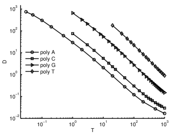
Figure 1: Dependencies of the diffusion coefficient $\mathrm{D}$ on temperature $\mathrm{T}$ for homogeneous nucleotides. Calculation results denoted by symbols are connected by line segments. The scales are logarithmic.

It turned out that upon rescaling $\mathrm{T}\to\mathrm{T}/\eta^{2}$, $\mathrm{D}\to\mathrm{D}/\eta$, all the graphs are similar, especially for low temperatures (see Fig. 2).

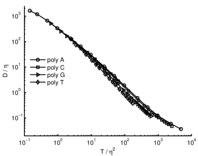
Figure 2: Rescaled dependencies for homogeneous polynucleotides.

It has been empirically found that for medium temperatures, rescaling $\mathrm{T}\to\mathrm{T}/\eta^{2}$, $\mathrm{D}\to\mathrm{D}/\sqrt{\eta}$ suits better. From Fig. 3 we notice that for rescaled temperature $\mathrm{T}/\eta^{2}>10$, all the graphs are very close to one another.

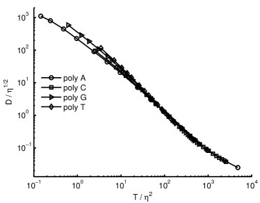
Figure 3: Other rescaled dependencies for homogeneous nucleotides. The temperature $\mathrm{T}$ is rescaled as in Fig. 1, but the diffusion coefficient $\mathrm{D}$ is divided by $\sqrt{\eta}$.

We approximated the data on a logarithmic scale by cubic polynomial for both the dependencies $\mathrm{D}_{1}=\mathrm{D}/\eta$ and $\mathrm{D}_{2}=\mathrm{D}/\sqrt{\eta}$ on different temperature intervals $\mathrm{T}_{1}=\mathrm{T}/\eta^{2}$, having chosen $0<\mathrm{T}_{1}\leq R\approx 8$ for the approximation interval $\mathrm{D}_{1}$, and $\mathrm{T}_{1}>R$ for $\mathrm{D}_{2}$. The obtained parameter values of the functions

$$y=a_{0}x^{3}+a_{1}x^{2}+a_{2}x+a_{3},\quad x=\ln(\mathrm{T}/\eta^{2}),$$ (9)

are as follows:

• for $y_{1}=\ln(\mathrm{D}/\eta)$, on the interval $0<\mathrm{T}/\eta^{2}\leq 8$,

  $$a_{0} =1.3359590\cdot 10^{-2}, a_{1} =-7.0449850\cdot 10^{-2},$$

  $$a_{2} =-1.0275530, a_{3} =5.7815836;$$

• for $y_{2}=\ln(\mathrm{D}/\sqrt{\eta})$, on the interval $8\leq\mathrm{T}/\eta^{2}$,

  $$a_{0} =1.4621272\cdot 10^{-2}, a_{1} =-1.7419911\cdot 10^{-1},$$

  $$a_{2} =-6.5194332\cdot 10^{-1}, a_{3} =5.4939738.$$

Graphs of approximating polynomials are shown in Fig. 4.

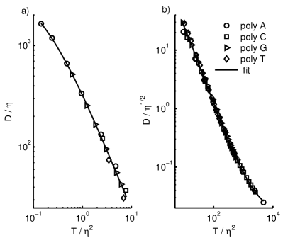
Figure 4: Results of modeling and graphs of approximating polynomials. a) Low temperatures, rescaling $\mathrm{T}\to\mathrm{T}/\eta^{2}$, $\mathrm{D}\to\mathrm{D}/\eta$, b) medium temperatures, rescaling $\mathrm{T}\to\mathrm{T}/\eta^{2}$, $\mathrm{D}\to\mathrm{D}/\sqrt{\eta}$.

The boundary value $R\approx 8$ is chosen in the following way. For the results from the intercept $\mathrm{T}_{1}\in[0,r]$, we calculated a summary deviation $S_{1}$ from the approximation curve $y_{1}(x)$, normalized by the number of results $K$, and on the second interval $r<\mathrm{T}_{1}$ we found the same deviation $S_{2}$ from $y_{2}(x)$:

$$S_{1} =\frac{1}{K}\sum_{k=1}^{K}[y_{1}(x_{k})-y_{1k}],\quad S_{2}=\frac{1}{L}\sum_{l=1}^{L}[y_{2}(x_{l})-y_{2l}].$$

With increasing $r$, $S_{1}$ grows and $S_{2}$ decreases. The abscissa of intersection of their graphs is chosen to be a boundary of partitions $R$.

V Extensions of the model. Taking account of stacking interaction in DNA

In DNA, of great importance is nonlinear stacking interaction $\Theta(\tilde{u}_{n}-\tilde{u}_{n-1})$ Komineas et al. (2002); Dauxois et al. (1993), which for small values of the difference has the form Komineas et al. (2002)

$$\Theta(\tilde{u}_{n}-\tilde{u}_{n-1})=\frac{1}{2}K_{s}\cdot(\tilde{u}_{n}-\tilde{u}_{n-1})^{2}.$$

More detailed Peyrard–Bishop model with nonlinear interaction between neighboring base pairs Peyrard and Bishop (1989); Dauxois et al. (1993) for the case of small site displacements can be reduced to the form similar to that of the dispersion term in equations for crystals.

Solvation effects play a great role in processes of charge transfer Basko and Conwell (2002a); Voityuk (2005).

Earlier Lakhno and Fialko (2012) we have calculated the hole mobility for polyG fragments of DNA in the cases of dispersion in classical chain and taking account of solvation effects. The total energy of the system has the form

$$\langle\Psi|\hat{H}|\Psi\rangle=\sum_{m,n}\nu_{nm}b_{m}b_{n}^{*}+\sum_{n}\alpha^{\prime}\tilde{u}_{n}b_{n}b_{n}^{*}$$

$$+\frac{1}{2}\sum_{n}\tilde{\Phi}(b_{n}b_{n}^{*})^{2}+\frac{1}{2}\sum_{n}K_{s}(\tilde{u}_{n}-\tilde{u}_{n-1})^{2}$$

$$+\frac{1}{2}\sum_{n}M\dot{\tilde{u}}_{n}^{2}+\frac{1}{2}\sum_{n}K\tilde{u}_{n}^{2}.$$

Here $K_{s}$ is a constant determining the contribution of dispersion into the chain energy. In molecular crystals, the value of dispersion $K_{s}$ in a classical chain is usually small. For DNA, this is not the case. For DNA in Komineas et al. (2002) the value of stacking interaction was found to be $K_{s}\approx 0.04$ eV/AA², and for intramolecular hydrogen bonds $K\approx 0.06$ eV/AA².

The energy of charge’s solvation on the $n$-th site depends on the charge distribution density on the site Neill et al. (2001), $\tilde{\Phi}$ is the effective solvation coefficient. In the calculations of diffusion coefficient we took $\tilde{\Phi}=1.04$ eV Voityuk (2005).

The dimensionless parameters are: $k_{s}=6.4\cdot 10^{-5}$, $\Phi=15.5$. In calculations of individual simulations we added random force and friction into motion equations of classical sites, as aforesaid.

Using an approximating curve obtained for medium temperatures (II), we considered an “inverse problem” as applied to temperature dependencies D(T), founded for model with dispersion and solvation.

I.e., for homogeneous chains we have found the cubic polynomial approximation (9) with coefficients $a_{i}$ from (II) in the coordinate system $x=\ln(\mathrm{T}/\eta^{2})$, $y=\ln(\mathrm{D}/\sqrt{\eta})$. Let us assume that for a certain chain (with dispersion or with solvation, or a regular chain), we can find an “effective” value of $\eta_{\mathit{eff}}$ such that upon rescaling, the graph D(T) for this chain will fall on this approximating curve (II).

This problem reduces to finding a minimum of the distance $R(\eta)$ from a point to the curve (II). We have data for one temperature (T,D). It is required to find $\eta$, such that the point with the coordinates $x_{0}=\ln(\mathrm{T}/\eta^{2}),y0=\ln(\mathrm{D}/\sqrt{\eta})$ be as close to curve (II) as possible. If $\eta_{\mathit{eff}}$ values obtained are close for different values T, then the graph will be similar to the graph of D(T) in a homogeneous chain with the matrix element $\eta_{\mathit{eff}}$.

The test of this assumption showed that in the parameter range under consideration: 1) For chains with dispersion ($k_{s}=6.4\cdot 10^{-5}$, $\Phi=0$) it is valid; 2) For chains with solvation, chains with solvation and dispersion and regular chains it is not valid.

For the first case, we calculated diffusion coefficient D(T) in all the homogeneous polynucleotide chains with dispersion. The $\eta_{\mathit{eff}}$ values were close for different temperatures. The D(T) in polyA fragment was found to be close to that in a homogeneous chain with $\eta_{\mathit{eff}}\approx 0.70$ (which corresponds to the matrix element $\nu\approx 0.046$ eV), for polyC $\eta_{\mathit{eff}}\approx 0.96$ ($\nu\approx 0.063$ eV); for polyG $\eta_{\mathit{eff}}\approx 2.08$ ($\nu\approx 0.137$ eV), and for polyT $\eta_{\mathit{eff}}\approx 4.1$ ($\nu\approx 0.270$ eV). The results of the calculations in chains with dispersion and in homogeneous chains with “effective” matrix elements $\eta_{\mathit{eff}}$ are shown in Figure 5. A considerable discrepancy for polyT at $\mathrm{T}\leq 150$ stems from the fact that the “boundary value” $R\approx 8$, below which another approximation (I) should be used, for $\eta=4.1$ corresponds to $\mathrm{T}=R\eta^{2}\approx 135$.

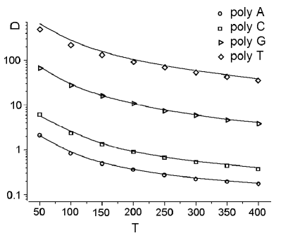
Figure 5: Dimensionless temperature dependencies of the mobility, ${\mathrm{T}}T^{*}=T$ [K], in semilogarithmic scale. Symbols stand for the values of the diffusion coefficient D, calculated for homogeneous chains with dispersion. Continuous lines going adjacently join the values of D(T) calculated for dispersionless chains (with the use of equations (4), (5)) with other matrix elements: near the values for polyA runs a curve with $\eta_{\mathit{eff}}=0.7$, near those for polyC is a curve with $\eta_{\mathit{eff}}=0.96$, near the values for polyG – a curve with $\eta_{\mathit{eff}}=2.08$, and near those for polyT – a curve with $\eta_{\mathit{eff}}=4.1$.

So, to find temperature dependence $\mathrm{D}(\mathrm{T})$ of the charge in the homogeneous chain with dispersion we may to calculate $\mathrm{D}$ for one value $\mathrm{T}$ and to count $\eta_{\mathit{eff}}$. Than, this $\eta_{\mathit{eff}}$ may be used for estimating $\mathrm{D}$ at different temperatures.

For homogeneous chains with solvation $\Phi=15.5$, we failed to find a common matrix element $\eta_{\mathit{eff}}$ for different temperatures (see Table 2).

We also calculated mobility for regular fragments of the form of …ATATAT… and …GTGTGT…. In calculations of individual simulations, integration was performed for the system of equations (4), (5), in which matrix elements depended on the sequence type and the sites of the classical subsystem were assumed to be similar. The values of matrix elements were taken from Voityuk et al. (2000); Jortner et al. (2002): $\nu_{\mathrm{AT}}=0.105$ eV ($\eta_{\mathrm{AT}}=1.595$), $\nu_{\mathrm{TA}}=0.086$ eV ($\eta_{\mathrm{TA}}=1.307$), $\nu_{\mathrm{GT}}=0.137$ eV ($\eta_{\mathrm{GT}}=2.081$), $\nu_{\mathrm{TG}}=0.085$ eV ($\eta_{\mathrm{TG}}=1.291$). Then we tried to fit $\eta_{\mathit{eff}}$, however $\eta_{\mathit{eff}}$ differs considerably for different temperatures (see Table 2).

Table 2: Results of $\eta_{\mathit{eff}}$ calculation for the minimum distance to the approximating curve (II). Value of the effective matrix element $\eta_{\mathit{eff}}$ for different temperature T.

Chain	T=100	T=200	T=300
polyG with solvation
($\Phi=15.5$, $k_{s}=0$)	0.33	0.28	0.22
polyG with dispersion and solvation
($\Phi=15.5$, $k_{s}=6.4\cdot 10^{-5}$)	0.62	0.57	0.53
…ATATAT…	0.77	0.82	0.88
…GTGTGT…	0.47	0.52	0.55

As can be seen from Table 2, for the case of chain with solvation we could not find a single value $\eta_{\mathit{eff}}$ for different temperatures. Also, the idea of $\eta_{\mathit{eff}}$ is not worked for regular polynucleotides.

VI Discussion

It is shown that the values of the diffusion coefficient $\mathrm{D}$ in a Holstein model chain simulating homogeneous DNA, which are different for different nucleotide types, being rescaled, fall on one and the same curve in the corresponding range $\mathrm{T}_{1}=\mathrm{T}/\eta^{2}$. For low $\mathrm{T}_{1}\leq 8$, rescaling is $\mathrm{D}\to\mathrm{D}/\eta$, for medium $T_{1}>8$, rescaling $\mathrm{D}\to\mathrm{D}/\sqrt{\eta}$ suits better. For these data on a logarithmic scale, approximating cubic dependencies are found.

In studying the charge mobility in system (4), (5), we were interested in a qualitative picture and left aside the domain of applicability of the model. The semiclassical model used cannot be applied at temperatures below Debye one $k_{B}T\leq\Theta=\hbar\omega$ (for model nucleotide pairs $\Theta\approx 8$ K). Calculations were carried out for coefficients that are similar at any temperature. This is a simplest assumption. Surely some parameters are temperature dependent. The most spectacular example is concerned with DNA whose constant of hydrogen bonds interaction $K\to 0$ as $T\to 350$ K (at temperature 60–80^∘C DNA melts and hydrogen bonds of complementary pairs are broken). It may be assumed that as the temperature decreases, the coefficient values change less and less and finally become a constant.

We considered the Holstein model of DNA where Watson–Crick pairs are represented as independent oscillators described by classical motion equations. It is believed that the planes of nucleotide base pairs are parallel to each other at any moment and the distances between neighboring planes are unchanged (the standard DNA model). The transfer of a hole in a DNA is determined by overlapping of its wave functions at neighboring sites. In view of the model geometry, the overlapping integrals are virtually independent of the displacements. Thus in Hamiltonian (1) we take into account the (intrasite) displacements for the diagonal matrix elements only.

In Su-Schrieffer-Heeger (SSH) model Su et al. (1979), the non-diagonal matrix element dependence on inter-site displacements is considered. SSH model has been applied to DNA by the Conwell et al. Conwell and Rakhmanova (2000); Basko and Conwell (2002b); Conwell et al. (2005). Two important degrees of freedom in DNA chain are relative base pair displacements along the stack and the relative twist angles. It was shown Basko and Conwell (2002b) that since these degrees of freedom are not independent they can be taken into account by introducing the dependence of the matrix elements on the inter-site displacements with effective coupling constant. SSH model was applied to describe the properties of polarons in DNA in many works (see e.g. Zeković et al. (2011); T.Koslowski et al. ; Koslowski and Cramer and references therein). In the work Lakhno and Fialko (2005) we calculated the hole mobility for Holstein model, SSH model and combined one (HSSH-model), in polyG at $T=300$ K. The values obtained were similar. It is task for further research to verify the scaling laws for SSH and HSSH DNA model.

We considered the simple case of the harmonic potentials in the classical chain of sites. Holstein model with dispersion exactly corresponds to the Peyrard–Bishop model for DNAPeyrard and Bishop (1989), when sites displacements from their equilibrium positions are smallDauxois et al. (1993). This should undoubtedly be valid for low temperatures, however at room and higher temperatures the assumption of the displacements smallness can be incorrect. In this case consideration of the Peyrard–Bishop model which takes account of the chain anharmonicity becomes actual. The authors are planning to study this problem in the future.

Based on the numerical results for Holstein semiclassical model, we can assume that charge mobility in molecular chain with dispersion and matrix element $\eta_{1}$ looks like mobility in chain without dispersion and matrix element $\eta_{2}$, and $\eta_{1}<\eta_{2}$. Also, the approximated cubic curve is not valid for regular chains and for homogeneous chain with solvation. The curve can be applied for estimation of the hole mobility in “dry DNA” rather than in “DNA in a solvent”.

We believe that in the range of “biologically significant” temperatures, for homogeneous biopolymers with parameters close to DNA parameters discussed, one can approximately assess the value of the charge mobility at temperature $T$ without carrying out resource-intensive model calculations, just by associating it with a point with suitable coordinate $\mathrm{T}_{1}$ and recalculating the diffusion coefficient.