Broadband monitoring tracing the evolution of the jet and disk in the black hole candidate X-ray binary MAXI J1659$-$152 

Abstract

MAXI J1659$-$152 was discovered on 2010 September 25 as a new X-ray transient, initially identified as a gamma-ray burst, but was later shown to be a new X-ray binary with a black hole as the most likely compact object. Dips in the X-ray light curves have revealed that MAXI J1659$-$152 is the shortest period black hole candidate identified to date. Here we present the results of a large observing campaign at radio, sub-millimeter, near-infrared (nIR), optical and ultraviolet (UV) wavelengths. We have combined this very rich data set with the available X-ray observations to compile a broadband picture of the evolution of this outburst. We have performed broadband spectral modeling, demonstrating the presence of a spectral break at radio frequencies and a relationship between the radio spectrum and X-ray states. Also, we have determined physical parameters of the accretion disk and put them into context with respect to the other parameters of the binary system. Finally, we have investigated the radio-X-ray and nIR/optical/UV-X-ray correlations up to $\sim 3$ years after the outburst onset to examine the link between the jet and the accretion disk, and found that there is no significant jet contribution to the nIR emission when the source is in the soft or intermediate X-ray spectral state, consistent with our detection of the jet break at radio frequencies during these states.

1 Introduction

Black hole X-ray binaries (BHXBs) are usually discovered as transient sources, with a large outburst in X-rays accompanied by increased emission at ultraviolet (UV), optical, near-infrared (nIR) and radio wavelengths (for a review, see e.g. McClintock & Remillard, 2006; Belloni, 2010; Fender, 2010; Gallo, 2010; Gilfanov, 2010). These systems spend most of their time in a quiescent state, where the optical/nIR emission is emitted by the companion star or the cool accretion disk. The flux across the electromagnetic spectrum increases by orders of magnitude during outbursts, which are powered by increased accretion onto the black hole and can last weeks to months. The radio emission in these outbursts is ascribed to a relativistic jet, and sometimes these sources are named microquasars by analogy to radio-loud active galactic nuclei (Mirabel et al., 1992).

During an outburst BHXBs go through several canonical X-ray spectral states, following a typical trajectory in the hardness-intensity diagram (HID; e.g. Homan et al., 2001; Homan & Belloni, 2005; Belloni, 2010). Typically, the source will first become significantly brighter while the spectrum is relatively hard and power-law dominated (hard state), after which the source will become spectrally soft and thermal dominated (soft state); and it eventually dims and evolves back to the hard and then quiescent states. The various spectral states can also be associated with different time variability behavior and the presence of certain types of quasi-periodic oscillations (QPOs; e.g. Wijnands, Homan & van der Klis, 1999; Casella, Belloni & Stella, 2005; Motta et al., 2011). There are various classifications in the literature for the different states, based on spectral and timing behavior. In this paper we follow Homan & Belloni (2005) and Belloni (2010) in identifying the hard-intermediate state (HIMS) and soft-intermediate state (SIMS) in between the hard and soft states (see McClintock & Remillard, 2006, for an alternative classification).

The X-ray emission is thought to be produced in the accretion disk and/or a hot corona above the disk, and the UV, optical and nIR emission is also produced in the accretion disk, either intrinsically (e.g. Shakura & Sunyaev, 1973) or by reprocessing of X-rays in that same region (e.g. van Paradijs & McClintock, 1994). At nIR to optical wavelengths there may also be a contribution from the jet that dominates the radio emission (e.g. Corbel & Fender, 2002; Russell et al., 2006). The latter emission is usually described by a flat spectrum and it is bright during the initial hard state. In some models there is also a contribution from the jet at X-ray frequencies (e.g. Markoff & Nowak, 2004). During the transition to the soft state the radio emission is quenched, and in some sources discrete ejecta are launched and their radio emission can be spatially resolved (e.g. Fender, Belloni & Gallo, 2004).

On 2010 September 25 a new transient was discovered with the Burst Alert Telescope (BAT) onboard the Swift satellite, which was initially identified as a gamma-ray burst (GRB) and named GRB 100925A (Mangano et al., 2010). The source was independently detected as a peculiar hard X-ray emitting source by the Gas Slit Camera (GSC) of the Monitor of All-sky X-ray Image (MAXI) instrument onboard the International Space Station, and was designated as MAXI J1659$-$152 (Negoro et al., 2010). Soon after its discovery it was realized that this new transient was not a GRB (Kann, 2010; Xu, 2010), and observations with the X-shooter spectrograph at the ESO Very Large Telescope (VLT) identified the source as an X-ray binary (de Ugarte Postigo et al., 2010a; Kaur et al., 2012). The nature of the source was confirmed by the Rossi X-ray Timing Explorer (RXTE), classifying it as a black hole candidate (Kalamkar et al., 2010) based on the identification of its low-frequency QPOs. MAXI J1659$-$152 evolved through the X-ray hardness-intensity diagram in a manner characteristic of low-mass X-ray binaries, and the presence of type-B and type-C QPOs, and the way in which they evolve during the outburst, have provided evidence for the black hole nature of the compact object (Kalamkar et al., 2011; Muñoz-Darias et al., 2011).

Further observations at X-ray and soft gamma-ray energies with Swift (Kennea et al., 2010), INTEGRAL (Kuulkers et al., 2010), RXTE (e.g. Belloni, Muñoz-Darias & Kuulkers, 2010), MAXI and XMM-Newton, have shown that there are dips in the light curves recurring at a period of $2.414\pm 0.005$ hours (Kuulkers et al., 2013). These have been interpreted as absorption dips at the orbital period of the system, which makes MAXI J1659$-$152 the shortest period black hole candidate known to date (Kuulkers et al., 2012, 2013; Kennea et al., 2011). For absorption dips to occur, the inclination angle of the accretion disk with respect to the line of sight is relatively well constrained at $\sim 65-80$°. This allows for an estimate of the binary orbital separation, and mass and radius of the donor star. The binary system appears to be compact (orbital separation of $>1.33~{}\rm{R}_{\odot}$) and the companion is suggested to be an M5 or M2 dwarf star (Kuulkers et al., 2013; Kong, 2012).

After the source discovery we initiated a broadband follow-up campaign. Besides many of the aforementioned observations at X-ray and soft gamma-ray energies, we observed the source in various UV, optical and nIR bands, and at sub-millimeter and several radio frequencies. A varying optical source was detected with the Swift UltraViolet and Optical Telescope (UVOT; Marshall, 2010), and in the R-band with BOOTES-2 and IAC80 (Jelinek et al., 2010), while optical variability on minute timescales was found with the Faulkes Telescope (Russell et al., 2010a). At sub-millimeter wavelengths MAXI J1659$-$152 was detected with the Atacama Pathfinder EXperiment (APEX; de Ugarte Postigo et al., 2010b), and at radio frequencies with the Westerbork Synthesis Radio Telescope (WSRT; van der Horst et al., 2010a). We followed the evolution of the outburst during various transitions at X-ray (Belloni, Motta & Muñoz-Darias, 2010; Shaposhnikov & Yamaoka, 2010; Muñoz-Darias et al., 2010) and radio (van der Horst et al., 2010c; Paragi et al., 2010) wavelengths.

Here we present the results of our observing campaign across the electromagnetic spectrum, focusing on the broadband modeling of several epochs for which we have well covered spectral energy distributions (SEDs) including observations at several radio frequencies, and on correlations between the different spectral regimes. In Section 2 we describe all our broadband observations and data analysis, and in Section 3 we present the resulting light curves. Our broadband spectral modeling is detailed in Section 4, while we discuss the radio-X-ray and nIR/optical/UV-X-ray correlations in the context of other BHXBs in Section 5. We summarize and conclude in Section 6. All uncertainties in measured quantities and modeling parameters are quoted at the $1\sigma$ confidence level.

2 Observations & Data Analysis

2.1 Radio

Table 1: Radio and sub-millimeter observations of MAXI J1659$-$152, with $\Delta$T the number of days after MJD 55464.0 (the source discovery date). WSRT^∗ indicates WSRT observations taken as part of EVN e-VLBI runs (Paragi et al., 2013). Upper limits are given at the $3\sigma$ level.

Epoch	$\Delta$T	Obser-	0.61 GHz	1.4 GHz	2.3 GHz	4.9 GHz	8.5 GHz	22 GHz	43 GHz	345 GHz
(MJD)	(days)	vatory	(mJy)	(mJy)	(mJy)	(mJy)	(mJy)	(mJy)	(mJy)	(mJy)
55464.96 $-$ 55465.08	1.02	APEX	…	…	…	…	…	…	…	15.8$\pm$3.0
55465.59 $-$ 55465.82	1.70	WSRT	…	…	…	5.39$\pm$0.05	…	…	…	…
55467.05 $-$ 55467.13	3.09	VLA	…	…	…	10.30$\pm$1.03	…	10.00$\pm$1.05	…	…
55467.17 $-$ 55467.34	3.25	ATCA	…	…	…	9.76$\pm$0.06	11.29$\pm$0.06	…	…	…
55467.51 $-$ 55467.83	3.67	WSRT	…	6.95$\pm$0.14	6.68$\pm$0.08	…	…	…	…	…
55468.05 $-$ 55468.13	4.09	VLA	…	…	…	9.88$\pm$0.30	10.03$\pm$0.31	11.81$\pm$0.71	11.19$\pm$0.59	…
55469.63 $-$ 55469.76	5.69	WSRT∗	…	…	…	9.77$\pm$0.10	…	…	…	…
55470.06 $-$ 55470.15	6.10	VLA	…	…	…	10.29$\pm$0.32	9.74$\pm$0.30	8.84$\pm$0.49	4.84$\pm$0.35	…
55471.50 $-$ 55471.82	7.66	WSRT	…	9.02$\pm$0.16	9.40$\pm$0.08	…	…	…	…	…
55471.98 $-$ 55472.06	8.02	VLA	…	…	…	9.23$\pm$0.28	7.55$\pm$0.42	7.88$\pm$0.42	3.74$\pm$0.40	…
55473.58 $-$ 55473.75	9.66	WSRT∗	…	…	…	3.65$\pm$0.09	…	…	…	…
55473.97 $-$ 55474.06	10.01	APEX	…	…	…	…	…	…	…	10.5$\pm$3.2
55475.95 $-$ 55476.07	12.01	APEX	…	…	…	…	…	…	…	$<$6.0
55476.48 $-$ 55476.80	12.64	WSRT	…	1.15$\pm$0.10	1.26$\pm$0.06	…	…	…	…	…
55476.96 $-$ 55477.04	13.00	VLA	…	…	…	0.63$\pm$0.03	0.59$\pm$0.03	0.41$\pm$0.07	$<$0.10	…
55479.90 $-$ 55480.05	15.97	APEX	…	…	…	…	…	…	…	$<$6.3
55480.97 $-$ 55481.01	16.99	VLA	…	…	…	0.59$\pm$0.03	0.65$\pm$0.06	…	…	…
55482.98 $-$ 55483.03	19.00	VLA	…	…	…	0.95$\pm$0.04	0.88$\pm$0.04	…	…	…
55484.46 $-$ 55484.78	20.62	WSRT	…	2.23$\pm$0.12	…	2.03$\pm$0.06	…	…	…	…
55488.37 $-$ 55488.49	24.43	GMRT	$<$0.42	…	…	…	…	…	…	…
55488.45 $-$ 55488.77	24.61	WSRT	…	$<$0.27	$<$0.23	…	…	…	…	…
55488.99 $-$ 55489.03	25.01	VLA	…	…	…	0.23$\pm$0.03	$<$0.069	$<$0.25	…	…
55494.31 $-$ 55494.52	30.42	GMRT	$<$0.15	…	…	…	…	…	…	…
55499.90 $-$ 55499.94	35.92	VLA	…	…	…	$<$0.072	$<$0.066	…	…	…
55554.64 $-$ 55554.69	90.66	VLA	…	…	…	0.081$\pm$0.016	…	…	…	…

We observed MAXI J1659$-$152 at radio and sub-millimeter frequencies ranging from 610 MHz to 345 GHz, using the WSRT, Karl G. Jansky Very Large Array (VLA), Australia Telescope Compact Array (ATCA), and Giant Metrewave Radio Telescope (GMRT). The results of our radio campaign are given in Table 1, and the upper panel of Figure 1 shows the light curves for four of our radio observing frequencies to illustrate the broadband radio evolution of the outburst.

Very Long Baseline Interferometry (VLBI) observations with the European VLBI Network (EVN) and Very Long Baseline Array (VLBA) are presented in Paragi et al. (2013). Resulting fluxes of these observations are not included here, since the source is resolved in those, but we have included the WSRT synthesis-array fluxes from the two EVN observations.

2.1.1 Very Large Array

We used the VLA to observe MAXI J1659$-$152 over multiple epochs at 5, 8, 22 and 43 GHz, starting on 2010 September 28 (MJD 55467) and ending on 2010 December 24 (MJD 55554), as detailed in Table 1. The VLA was in the DnC configuration (maximum baseline of 1.9 km) for the observations from 28 September to 2 October, and in the C configuration (maximum baseline of 3.4 km) from 7 October through the end of our observations. We used the new WIDAR correlator with 2 sub-bands and 64 channels per sub-band covering a bandwidth of 128 MHz (i.e., 256 MHz in total). We selected 3C286 for our absolute flux calibrator and used two nearby calibration sources, J1707$-$1415 and J1658$-$0739, to apply complex gain calibration. For polarization measurements, we used OQ208 as our leakage calibrator.

We performed all of our calibration and reduction in the Astronomical Image Processing System (AIPS; Wells, 1985), using standard procedures for radio frequency interference excision, spectral channel selection, and calibration. For estimating the systematic uncertainties in our measured flux densities, we went by the guidelines outlined in the VLA Calibrator Manual. We added in quadrature systematic uncertainties of 3% (4.9 and 8.5 GHz) and 5% (22 and 43 GHz) of the measured flux densities. As with any new instrument, we experienced some “teething trouble” with the VLA. Our first observing run produced little useful data. We only managed to get time on MAXI J1659$-$152 but had no time on 3C286 for flux calibration and only 1 scan per band on J1658$-$0739. We used measurements of J1658$-$0739 from our second observing run to bootstrap fluxes from the first run. We also missed 3C286 at 8.5 GHz during our observing run on 2010 October 11 (MJD 55480) and had to bootstrap the flux calibration using J1707$-$1415. These problems resulted in significantly higher uncertainties for these two observations.

We determined the degree of polarization in our 5 and 8 GHz observations in the first two weeks of the outburst. We did not detect any significant polarization in our measurements, with 3$\sigma$ upper limits varying from 1% to 5% in the first three epochs, and tens of percent in the fourth epoch. At later epochs the polarization limits are less constraining due to the reduced brightness of the source.

2.1.2 Westerbork Synthesis Radio Telescope

We performed observations of MAXI J1659$-$152 with the WSRT at 1.4, 2.3 and 4.9 GHz, using the Multi Frequency Front Ends (Tan, 1991) in combination with the IVC+DZB back end in continuum mode, with a bandwidth of 8x20 MHz at all observing frequencies. Complex gain calibration was performed using the calibrator 3C286 for all observations. The observations were analyzed using the Multichannel Image Reconstruction Image Analysis and Display (MIRIAD; Sault, Teuben & Wright, 1995) software package, except for the WSRT data that were obtained during VLBI observations, which were analyzed with AIPS. The flux uncertainties were determined with the MIRIAD task imfit, to which the rms noise in the image around MAXI J1659$-$152 was added in quadrature.

With the initial discovery of the radio counterpart of MAXI J1659$-$152 we also reported a high degree of linear polarization in the source (van der Horst et al., 2010a). However, careful re-analysis of this first epoch, and also analysis of the other WSRT epochs at 4.9 GHz, does not show any significant polarization, consistent with the non-detections of polarized emission with the VLA.

2.1.3 Australia Telescope Compact Array

MAXI J1659$-$152 was observed with the ATCA for 4.5 hours on 2010 September 28 (MJD 55467). We used the Compact Array Broadband Backend (CABB; Wilson et al., 2011) to observe simultaneously in two separate frequency bands, centered at 5.5 and 9.0 GHz. Each frequency band comprised 2048 channels, each of width 1 MHz, for a total observing bandwidth of 2048 MHz. The array was in its H75 configuration, with five closely-spaced antennas within 82 m, and a more distant sixth antenna 4.4 km away.

Data were converted to fits format using the MIRIAD software package, and then read into the Common Astronomy Software Applications (CASA) package for data editing, calibration and imaging. We used PKS 1934$-$638 as the primary calibrator, and J1733$-$1304 as the secondary calibrator. One of the central antennas was shadowed during observations of the primary calibrator, so had to be flagged. After editing out bad data and performing external gain calibration, we made a naturally-weighted image of the field containing MAXI J1659$-$152, using the multi-frequency synthesis algorithm in CASA to accurately deconvolve sources with non-zero spectral slopes. Owing to the large hole in the uv-coverage arising from the isolation of the sixth antenna, we only used data from the inner antennas during the imaging process, providing an angular resolution of 65 and 42 arcsec at 5.5 and 9.0 GHz, respectively. However, a comparison with higher-resolution VLA data shows that there were no bright confusing sources within these large beams, so the relatively poor angular resolution should not affect our photometry.

A second observation was made on 2010 October 1 (MJD 55470), with a central frequency of 2.1 GHz. Owing to the RFI affecting the majority of the observing bandwidth, and to the short duration of the observation (1.5 hours), we were unable to use these data to place any accurate constraints on the brightness of the target source.

2.1.4 Giant Metrewave Radio Telescope

GMRT observed the field of MAXI J1659$-$152 on 2010 October 19 and 25 (MJD 55488 and 55494, respectively) at an observing frequency of 610 MHz. Radio sources 3C286 and J1626$-$298 were used as flux and phase calibrators, respectively. The flux calibrator was observed for about 15 minutes at the start of the target observations. The phase calibrator and the field of MAXI J1659$-$152 were then observed alternately for 6 and 45 minutes. The analysis of the observations was carried out using AIPS, and resulted in non-detections at this frequency.

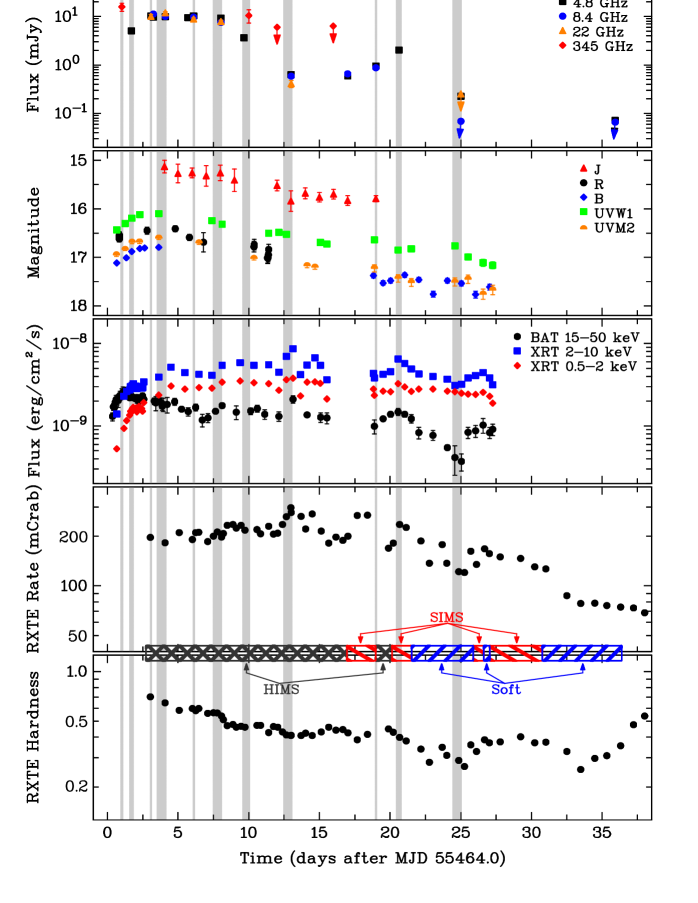
Figure 1: Light curves at various radio and sub-millimeter wavelengths (top panel), in nIR/optical/UV bands (2nd panel from the top), from Swift/BAT and Swift/XRT (middle panel), and from RXTE ($2-15$ keV; 2nd panel from the bottom); and the RXTE hardness ratio ($6-15$ keV/$2-6$ keV; bottom panel). The vertical grey bars indicate the epochs for which we performed broadband SED modeling. The times when the source was in the various X-ray states (HIMS, SIMS or soft state) are also indicated (following Muñoz-Darias et al., 2011). Note that the source was in the hard state in the first hours after the outburst onset, but the exact transition from hard state to HIMS is unknown due to the lack of RXTE observations.

2.2 Sub-millimeter

Continuum observations at 870 $\mu$m (i.e., 345 GHz) were carried out using the Large APEX BOlometer CAmera (LABOCA; Siringo et al., 2009) installed on the Atacama Pathfinder EXperiment (APEX; Lundgren et al., 2010). Data were acquired at four epochs under good weather conditions (zenith opacity values ranged from 0.17 to 0.43 at 870 $\mu$m). Observations were performed using the wobbler on-off mode and data were reduced using the Bolometer Array (BoA) analysis software. The total on-source integration time of the four epochs was 8.6 hr. The telescope pointing was checked every hour, finding an rms pointing accuracy of 2.1 arcsec. Calibration was performed using observations of the primary calibrators Mars, Uranus and Neptune, as well as the secondary calibrators G10.62, IRAS16293 and G5.89. The absolute flux calibration uncertainty is estimated to be 11%.

2.3 Near-Infrared, Optical & Ultraviolet

The nIR (J- and H-band) observations were performed using the 1.3m telescope (previously the 2MASS southern telescope) at the Cerro Tololo Inter-American Observatory (CTIO), which is currently operated by the Small & Moderate Aperture Research Telescope System (SMARTS) consortium (Subasavage et al., 2010). We observed MAXI J1659$-$152 with an almost daily cadence between 2010 September 29 (MJD 55468) and October 14 (MJD 55483). The data were recorded by a Rockwell HgCdTe Astronomical Wide Area Infrared Imager. Multiple dithered frames were taken and then flat-fielded, sky subtracted, aligned, and average-combined using an in-house IRAF script. We used two nearby 2MASS stars in the field of MAXI J1659$-$152 as references. The average magnitudes of these comparison stars were used as a basis for differential photometry with respect to MAXI J1659$-$152. Additional late-time deep observations in the J-band were carried out with the 3.5m CAHA telescope on 24 July 2013 (MJD 56497) with a total integration time of 38 minutes, resulting in a significant detection of $21.05\pm 0.17$ mag, $\sim 3$ years after the outburst onset.

Optical observations were carried out with the IAC80, 1.23m CAHA, 2.2m CAHA, 2.0m Liverpool, BOOTES-2/Telma and BOOTES-3/Yock-Allen telescopes. The IAC80 telescope is a 0.82m aperture facility, and the observations were done with the CAMELOT camera which is based on a 2k$\times$2k E2V CCD providing a pixel scale of 0.3 arcsec/pixel. The 1.23m CAHA, BOOTES-2/Telma and BOOTES-3/Yock-Allen facilities are Ritchey-Chretien telescopes. The 1.23m CAHA data were acquired with a 2048$\times$2048 SITE#2b CCD which yields a pixel scale of 0.5 arcsec/pixel. Both BOOTES stations are equipped with identical cameras, an Andor iXon-889+ electron multiplying CCD of 1024$\times$1024 pixels, with a pixel scale 0.6 arcsec/pixel (see Castro-Tirado et al., 1999, for more details on the BOOTES network of telescopes). The IAC80 and the 1.23m observations were carried out using standard Johnson/Cousins filters (Fukugita, Shimasaku & Ichikawa, 1995), while the images of both BOOTES stations were acquired using Sloan filters (Fukugita et al., 1996).

The 2.0m Liverpool Telescope (LT) observations were made in the SDSS $i^{\prime}$-band with RATCam, which yields a pixel scale of 0.135^′′/pix based on a 2048x2048 pixel EEV CCD42-40. Additional $g^{\prime}r^{\prime}i^{\prime}z^{\prime}$-band observations were carried out with the 2.2m Calar Alto telescope equipped with BUSCA. BUSCA is a multichannel camera which allows simultaneous direct imaging in four optical bands using three CCD485 Lockheed Martin plus one CCD485 backside thinned CCD (in the uv channel). The BUSCA observations were done in 2$\times$2 binning and 1k$\times$1k windowing mode, yielding a pixel scale of 0.35 $\arcsec$/pix and a field of view of 6$\arcmin\times 6\arcmin$.

The reduction of all the optical data was performed using standard procedures implemented in IRAF. Calibration of the Sloan data was carried out transforming the Johnson magnitudes of 22 field stars based on Jordi, Grebel & Ammon (2006). The source looks relatively isolated in optical images: there are no entries in either the 2MASS (Skrutskie et al., 1995) or USNO-B1.0 (Monet et al., 2003) catalogues consistent with the position of MAXI J1659$-$152. Furthermore, observations with the Canada-France-Hawaii Telescope at $\sim 18$ months after the start of the X-ray outburst result in a quiescent $r$ band magnitude of $\sim 23.6$ (Kong, 2012). We hence assume that the flux at the time of our analysis was dominated by the transient emission of MAXI J1659$-$152.

Data from the Swift UV/Optical Telescope were downloaded from the HEASARC archive and pre-processed at the Swift Data Center (see Breeveld et al., 2010), and required only minimum user processing with the Swift FTOOLS as follows. The image data from each filter, from each observation sequence, were summed using uvotimsum. Photometry of the source in individual sequences was derived via uvotmaghist, using an extraction region of radius 5″. XSPEC compatible spectral files were created with that same region using uvot2pha. The obtained magnitudes are based on the UVOT photometric system (Poole et al., 2008).

In Table 2 we give the results of our ground-based optical follow-up campaign and the Swift/UVOT observations.

2.4 X-rays

The outburst of MAXI J1659$-$152 was observed by several X-ray satellites and instruments. In this paper we focus on the Swift, RXTE and MAXI observations.

The light curves and spectra of the Swift X-Ray Telescope (XRT) were obtained from the XRT online tool, which offers science grade products (Evans et al., 2009). Swift Burst Alert Telescope (BAT) data were downloaded from the HEASARC archive and initially processed with the FTOOL batsurvey, which applies standard corrections. 8-channel spectra and response files were extracted and the standard spectral systematic error correction applied with batphasyserr. All X-ray spectra were binned to have $\geq 20$ counts per bin (with grppha) so that errors would be approximately Gaussian and hence $\chi^{2}$ statistics would be valid.

We analyzed all 65 observations of MAXI J1659$-$152 in the RXTE archive. For each observation we extracted a background and dead-time corrected energy spectrum from the PCA standard mode, using only data from Proportional Counter Unit (PCU) 2 of the PCA, as it is the best calibrated and the only one which is always active. We used the standard HEASOFT RXTE software to create energy spectra. From these spectra, we extracted background-corrected count rates in the PCA channel bands $A=0-35$ ($2-15$ keV; total band), $B=0-13$ ($2-6$ keV; soft band) and $C=14-35$ ($6-15$ keV; hard band). The RXTE rate $A$, converted to Crab units for PCU 2 (conversion factor of 1 Crab $=$ 2284 counts/second), was used as RXTE rate in Figures 1 and 6, while the hardness was defined as the ratio $C/B$.

The daily count rate ($2-20$ keV) and hardness ($4-10$ keV / $2-4$ keV) as measured by the MAXI instrument have been taken from the MAXI website.

3 Broadband Light Curves

Figure 1 shows a broadband overview of the light curves that we obtained in our follow-up campaign of MAXI J1659$-$152. In this figure we show the light curves at various radio frequencies, nIR, optical and UV bands, and X-ray and soft gamma-ray energies, from the observations presented in Section 2. We do not show light curves in all observing bands to avoid cluttering, but these selected observing bands illustrate the broadband evolution of the MAXI J1659$-$152 outburst well. For comparison we also show the RXTE count rate light curve and hardness evolution, and indicate the times when the source is in the various X-ray states (HIMS, SIMS or soft state), following the identification of these spectral states for MAXI J1659$-$152 by Muñoz-Darias et al. (2011). We note that the source was only in the hard state during the first hours after outburst onset, before the start of the RXTE observations. Because there are no RXTE observations during the first two days, we can not identify the exact time of the transition between the hard state and the HIMS.

It can be seen in Figure 1 that the source evolved in different ways in the various parts of the electromagnetic spectrum. In almost all wavebands we witnessed the rise of the source brightness, except for our APEX sub-millimeter observations which do not have the required temporal sampling, and the nIR observations which started around the peak of the outburst at those wavelengths. The observed trends in the optical, UV and X-ray light curves have been described in Kennea et al. (2011), with a correlated fast rise and slow decay at these frequencies, while the late-time X-ray behavior has been discussed in Homan et al. (2013). At radio frequencies the source was already fairly bright at 1.7 days after the start of the outburst (MJD 55464.0), and reached maximum brightness around day 3. During the following 5 days the radio brightness was constant, after which there was a sudden large decrease of the radio emission (van der Horst et al., 2010c). This radio flux drop was followed several days later by a transition from the hard-intermediate to the soft-intermediate state at X-ray energies (Belloni, Motta & Muñoz-Darias, 2010), and the radio flux started rising again after that. Other BHXBs have shown that at the transition to the SIMS, fast radio jets in the form of optically thin, discrete ejecta may emerge. This has, however, not been seen for MAXI J1659$-$152 (Paragi et al., 2013). After the second rise, the flux dropped significantly again at day 20 after the beginning of the outburst, and subsequently it was only detected at very low flux levels (Miller-Jones et al., 2011; Jonker et al., 2012).

4 Broadband Spectral Modeling

Given our rich broadband data set we performed broadband SED modeling. The grey vertical bands in Figure 1 indicate the 11 epochs for which this was done. We made our selection of the epochs based on the times for which we had radio data available. In the X-ray bands we used Swift/XRT and Swift/BAT data.

The broadband radio-to-X-ray spectra were fit within XSPEC (12.7.1), using $\chi^{2}$ statistics and accounting for interstellar extinction and absorption, which were modeled by redden and tbabs, respectively. The observed radio and optical flux densities $F_{\nu}$ at frequency $\nu$, were converted to flux per filter, $F_{\rm{filter}}$ in units of photons cm^-2 s^-1. This was done via $F_{\rm{filter}}=1509.18896F_{\nu}$ $(\Delta\lambda/\lambda)$, where $\lambda$ and $\Delta\lambda$ are the effective wavelength and width of respective filters. This flux was then used to produce XSPEC compatible files for spectral fitting, using the FTOOL flx2xsp.

At all epochs the data were well fit by a phenomenological broken power law at radio frequencies, and by a physically motivated irradiated disk model (diskir) at optical/UV and X-ray frequencies (Malzac, Dumont & Mouchet, 2005; Gierliński, Done & Page, 2008, 2009). In the latter model the X-ray emission consists of thermal emission from the accretion disk and a hard tail caused by Comptonisation of soft seed photons in a hot plasma of energetic electrons. The Comptonised emission in turn illuminates the disk, of which a large fraction gets reflected, but also a significant fraction of the photons are reprocessed and add to the disk emission. The parameters of this model are: the unilluminated disk temperature $kT_{disk}$; the power-law photon index $\Gamma$ of the Compton tail; the ratio of luminosity in the Compton tail to that in the unilluminated disk, $L_{C}/L_{disk}$; the fraction of bolometric flux which is thermalised in the outer disk, $F_{out}$; the log of the ratio of outer to inner disk radius, $r_{out}$; and a normalisation, $Norm$, dependent on the apparent inner disk radius. We note that it has been shown that spectra can be fit by an irradiated disk model even in the hard state (e.g. Miller, Homan & Miniutti, 2006; Rykoff et al., 2007).

The $\chi^{2}_{\nu}$ of the fits presented in the next section ranges from 1.1 to 2.0 for $\sim 10^{3}$ degrees of freedom, which are relatively high but given the disparity of the data (combination of many different instruments, epochs and bands) we deemed those acceptable. Furthermore, any variations from the model show no underlying structure, only noise-like variations.

Figure 2: Radio spectra of MAXI J1659$-$152 for the 6 epochs for which we have at least 3 observing bands. The lines indicate the (broken) power-law fits to the radio spectra. The solid and dashed lines for the spectrum at day 13 show the fits with and without including the low-frequency WSRT data below 3 GHz.

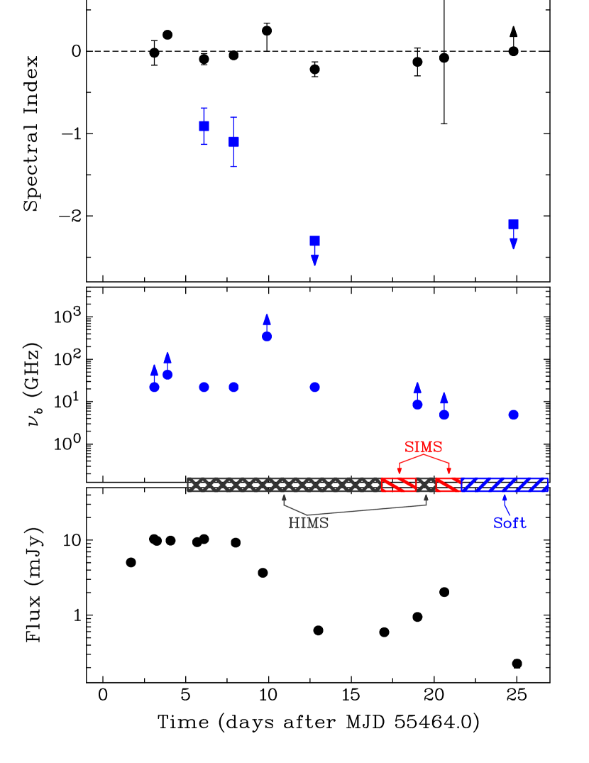
Figure 3: Evolution of parameters from the broken power-law fits to the radio SEDs indicated in Figure 1 except for the first two epochs. The top panel shows the spectral index, with the black circles indicating the low frequency power-law slopes, and the blue squares the high frequencies in those epochs that are best described by a broken power law. The middle panel shows the evolution of the spectral break for all epochs, including those for which we can only put upper or lower limits. In the lower panel the $4.9$ GHz light curve and the X-ray spectral states are displayed for comparison purposes.

4.1 Modeling Results

In our modeling the radio emission and the nIR to X-ray emission appear to be due to separate components. Figure 2 shows the radio spectra for 6 of our 11 epochs for which we have at least 3 radio bands. The behavior of the radio SEDs seems more complicated than a single flat or slightly-inverted spectrum across all radio bands (i.e. a spectral index $\sim~{}0$). We performed single and/or broken power-law fits to the radio SEDs for the epochs indicated in Figure 1 except for the first two epochs in which there was only one observing frequency. From Figure 2 it can be seen that there are epochs where a single power law is not sufficient to describe the spectrum, which is the case for 4 out of the 9 epochs we fit. For the latter epochs we show both spectral indices in Figure 3, while for the other 5 epochs we only show a single spectral index. In the broken power law fits we fixed the break at 22 GHz for the SEDs at 6, 8 and 13 days after MJD 55464.0, while at 25 days it was fixed at 4.9 GHz. In the former three epochs these break frequencies were fixed because the spectrum is consistent with a single power law up to 22 GHz and there is only one data point at 43 GHz to constrain the break, which makes the parameters of a free broken power-law fit hard to constrain. In fact, the break could be at any frequency in between 22 and 43 GHz and thus the high-frequency spectral indices can be steeper that the ones plotted in Figure 3. At day 25 there is only one detection at 4.9 GHz, hence the lower limit on the low-frequency spectral index and the upper limit on the high-frequency spectral index. We would like to point out, however, that the observations are not strictly simultaneous, so the 4.9 GHz detection could be a short flare with a timescale of hours. For those epochs where a break is not required at radio frequencies, we show lower limits on the break frequency in Figure 3. In our broadband radio-to-X-ray fits we placed those breaks arbitrarily at $10^{-5}$ keV ($\approx 2.4\times 10^{12}$Hz), with a steep cut-off.

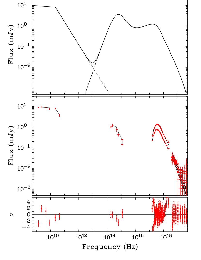
Figure 4: Example model plots for the broadband SED at day 8 after the outburst onset. The top panel shows the spectrum of the best fit model for this particular epoch, with the dotted line showing the broken power-law fit to the radio data, the dashed line the irradiated disk model fit, and the solid line the total spectrum. The middle panel shows the fit of the unfolded spectrum, with the data in red symbols and the best fit model in black lines. In the bottom panel we show the deviations from the best fit model.

An example fit to one of the epochs and the broadband model used here are shown in Figure 4. $E(B-V)$ displays no significant variability with an average of $0.595\pm 0.008$, consistent with the Galactic value of $E(B-V)=0.599$ (Schlegel, Finkbeiner & Davis, 1998). This is significantly larger than the value of $E(B-V)\simeq 0.35$ derived by Kaur et al. (2012). The measured values of interstellar absorption are consistent with being constant with an average of $N_{{\rm H}}=(0.319\pm 0.009)\times 10^{22}$ cm^-2. This value is greater than the expected Galactic absorption of $N_{{\rm H}}=0.17\times 10^{22}$ cm^-2 (Kalberla et al., 2005) but less than that obtained by Kennea et al. (2011). It should be noted, however, that Kennea et al. (2011) fit a different model and only to the X-ray data, while we include nIR/optical/UV data which add additional constraints to the thermal emission.

Figure 5 shows the evolution of the well-constrained parameters of the irradiated disk model. Although the fit parameter values we obtain are slightly different than the ones from Kennea et al. (2011) and Yamaoka et al. (2012), the trends in their evolution are similar. The disk temperature, $kT_{disk}$, rises from an initial temperature of $0.13$ keV to a relatively stable value of $\sim 0.3$ keV, while the photon index of the tail rises from an initial value of $\sim 2.0$ to a peak of $\sim 3.6$. As the disk temperature rises, the contribution that the Compton tail makes to the disk luminosity, $L_{C}/L_{disk}$, decreases, although this is poorly constrained on many epochs, and at late times is consistent with zero. Likewise, the fraction of bolometric flux which is thermalised in the outer disk, $F_{out}$, decreases although this is also poorly constrained. Since $L_{C}/L_{disk}$ and $F_{out}$ are poorly constrained, we have not plotted them in Figure 5. The ratio of outer to inner disk radius, $r_{out}$, increases with time which is due to the fact that the inner disk radius is decreasing. Instead of displaying $r_{out}$ and $Norm$, we show the physical inner radius $R_{in}$ and outer radius $R_{out}$ in Figure 5. The physical radius $R_{in}$ is related to the apparent radius $r_{in}$ of our fit by $R_{in}\approx 1.19r_{in}$ (see, e.g. Soria, 2007). We have determined $r_{in}$ at all the epochs from the fit values of $Norm$, assuming a source distance of 6 kpc (see Section 5) and an inclination of 70^∘. $R_{out}$ was derived from $R_{in}$ and the ratio $r_{out}$. In the next section, we will discuss further the trends in the fitted parameters.

Figure 5: Evolution of the disk temperature (top left), photon index of the Compton tail (bottom left), outer disk radius (top right), and inner disk radius (bottom right). These parameters are based on spectral fits to the broadband SEDs indicated in Figure 1, using the irradiated disk model.

4.2 Implications of Spectral Modeling

4.2.1 Radio SEDs & Spectral Breaks

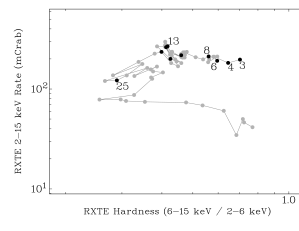
Figure 6: Hardness-intensity diagram for the RXTE (top) and MAXI (bottom; up to MJD 55515) data. The black dots indicate the epochs of X-ray observations for which we have (quasi-) simultaneous radio data. We have indicated the epochs on days 3, 4, 6, 8, 13 and 25 from the radio spectra shown in Figure 2. Note that RXTE was not observing MAXI J1659$-$152 from the outburst onset, hence there is one less black dot in the top panel compared to the bottom panel.

In this paper we present several epochs with broadband radio SEDs. To help place our SED epochs in the overall context of the behavior of the outburst, we indicate them on the HIDs of both the RXTE and MAXI data (Figure 6). In this figure we have indicated the X-ray observation epochs for which we performed broadband SED modeling with (quasi-) simultaneous radio data. MAXI J1659$-$152 was already in the HIMS when the RXTE observations started, but from the MAXI HID we can deduce that the source was transitioning from the hard state to the HIMS during the first radio observations, $1-2$ days after the outburst onset. Our first radio SED with good broadband coverage is at $\sim 3$ days after the onset of the X-ray outburst. The radio spectral index $\alpha$, where $F_{\nu}\propto\nu^{\alpha}$, is flat or inverted during the first 10 days over more than an order of magnitude in observing frequency, namely from 1.4 to 22 GHz, as one would expect from a synchrotron emitting, partially self-absorbed jet (Fender, 2001) and in full agreement with the observed VLBI structure (see Paragi et al., 2013, and the references therein). The spectrum is not constant over that time span though, with an inverted spectrum at day 4 with $\alpha=0.20\pm 0.02$, while it is flat at other epochs (see Figure 3). More striking is the sharp spectral break between 22 and 43 GHz that we find on days 6 and 8. After $\sim$10 days the radio flux drops significantly, but the spectrum is inverted even up to the sub-millimeter bands.

At day 13 the spectrum appears more complicated, with a sharp spectral break above 22 GHz, and a best-fitting spectral index of $\alpha=-0.49\pm 0.07$ at lower frequencies. We note, however, that the 1.4 and 2.3 GHz WSRT data were taken roughly 8 hours prior to the higher-frequency VLA data used to construct the spectrum shown in Figure 2, and since the source was undergoing a rapid decay, may have overestimated the true low-frequency emission at the time of the VLA observations. Furthermore, any variations from a compact, partially self-absorbed jet will be detected later at lower frequencies, since the lower-frequency emission comes from further downstream in the jets. Thus, for a rapidly-decaying compact jet, we might expect the lowest-frequency emission to be slightly overestimated, relative to the power law seen at higher frequencies. Combined, these two effects could explain the deviation of the low-frequency spectrum on day $\sim 13$ from a pure power law. To mitigate against this effect, we refitted the radio spectrum using only the VLA data between 4.9 and 22 GHz, to give a low-frequency spectral index of $\alpha=-0.22\pm 0.09$, with a break to $\alpha<-2.3$ above 22 GHz.

When the radio flux increases again and the source moves into the SIMS, the spectrum remains flat, but we do not have the spectral coverage at high radio frequencies to check for a spectral break. The radio measurements at day 25 are also consistent with being flat or inverted, but then with a sharp break in between 4.9 and 8.5 GHz.

From the radio light curves in Figure 1 and the spectral index evolution in Figure 3 it appears that the decrease in the radio emission around day 13 after the outburst onset did not coincide with a significant steepening of the spectrum, as observed in other BHXBs (e.g. Kuulkers et al., 1999; Fender, Belloni & Gallo, 2004; Miller-Jones et al., 2012). The low-frequency radio emission remained consistent with a partially self-absorbed compact jet throughout the HIMS, with no evidence for ejection events, in agreement with the absence of ejecta in the VLBI images of Paragi et al. (2013).

At higher frequencies, however, the radio spectrum exhibited a high-frequency break above 22 GHz from day $\sim 6$ until at least day $\sim 13$, and the optically thin spectrum appeared to steepen with time. This spectral break can be interpreted as the transition from optically thick and partially self-absorbed to optically thin synchrotron emission, and has previously been observed in several other BHXBs in hard X-ray states although usually at much higher frequencies (Russell et al., 2013a). Recently, Russell et al. (2013b) have shown that the BHXB MAXI J1836$-$194 has an inverted spectrum with a break towards a steep spectrum moving from the mid-infrared to lower frequencies as the source softens in the X-ray regime, and then back to higher frequencies as it gets harder again. With sufficiently dense monitoring over a broad radio frequency range one could be able to see the spectral break pass through the radio bands, which may explain what is happening between days 6 and 13 in MAXI J1659$-$152 (i.e. the inverse of what was seen during the reverse transition in GX339-4 by Corbel et al., 2013b). There appears to be a relatively rapid increase in the break frequency on day 10, shifting up to $>345$ GHz briefly before dropping back to 22 GHz on day 13. Since this is based on a spectrum consisting of flux density measurements at two frequencies, 4.9 and 345 GHz, this break frequency limit is quite uncertain. An inverted spectrum would shift it to a lower value, e.g. with a spectral index of 0.5 the break is at $\sim 170$ GHz, lower than the limit of 345 GHz but still significantly larger than 22 GHz. Nonetheless, the evolution of the break frequency at that time is fast, but this is not unprecedented: in GX 339-4 the spectral break shifted in the mid-infrared by more than an order of magnitude on timescales of hours when it was in the hard state (Gandhi et al., 2011). Given that the radio-emitting part of the jet is significantly larger than the infrared-emitting region, strong variability on a timescale of days in the case of MAXI J1659$-$152 could be expected. Alternatively, this could be a short-lived flare at sub-millimeter frequencies. Flares get smoothed out and have reduced amplitude at lower frequencies, which could explain the lack of a flare at 4.9 GHz.

The radio light curve shows an increase in flux between day 17 and 21, while the spectrum remains flat. In Figures 1 and 3 it can been seen that this coincides with a state transition (back and forth between the SIMS and the HIMS), consistent with what has been found for other BHXBs (e.g. Corbel et al., 2013b, a; Russell et al., 2013b). From these observations it seems that the jet started quenching in the HIMS and finished in the SIMS, but then recovered through a second HIMS and peaked in the second SIMS phase, before quenching again after a transition into the soft state. These changes in the radio emission coming from the jet and the X-ray state changes suggest a strong link between the accretion flow and the jet. It also shows that reaching the SIMS is no guarantee of a full transition to a jet ejection event, because there is no major radio flare when the sources moves into the soft state, and no discrete ejecta were detected in the VLBI observations (Paragi et al., 2013). Some other BHXBs in outburst also did not have ejection events, for instance Cyg X$-$1 (Rushton et al., 2012), but that source did not trace out a canonical track in the HID, while MAXI J1659$-$152 did (Muñoz-Darias et al., 2011). The soft state in MAXI J1659$-$152, however, was slightly harder than seen in BHXBs with ejection events, and the minimum fractional variability in the soft state was slightly higher (a minimum of 3%, and rising to 8% when the X-ray emission was softest; Muñoz-Darias et al., 2011). The authors attributed this to the high inclination of the system, but if it was instead intrinsic, the implied difference in the behaviour of the accretion flow could be related to the lack of jet ejection events. Miller-Jones et al. (2012) have shown, however, that the ejection event occurs well before reaching the soft state, at the HIMS/SIMS transition (see also Fender, Homan & Belloni, 2009). Since the behaviour of MAXI J1659$-$152 was relatively standard in the HIMS and SIMS, it seems unlikely that the unusual behaviour in the soft state could be causally related to the lack of ejection events.

4.2.2 Physical Constraints from the Irradiated Disk Model

In Figure 5 we show the evolution of the parameters of the irradiated disk model, in particular the disk temperature, the photon index of the Comptonised tail, and the inner and outer radius of the accretion disk. From this figure we can see that the source is getting spectrally softer (steeper photon index), the disk temperature is increasing, and the inner radius is decreasing, while the outer radius is fairly constant. The latter is not true for the first and sixth epoch, where we have only few nIR/optical data points to constrain the outer radius reliably. Excluding those epochs, the outer radius has a value of $\approx 0.9-1.6\times 10^{6}$ km, physically realistic considering the orbital separation (Kuulkers et al., 2013) and consistent with the position of the Lagrangian point $>10^{6}$ km. The inner radius of the disk is decreasing in time from $\sim 890$ to $\sim 110$ km, as one would expect in the standard picture of the disk evolution during a BHXB outburst. From the final value of $R_{in}$ (at day 25 after the outburst onset) we can put an upper limit on the black hole mass by assuming that $R_{in}$ is larger than the innermost stable circular orbit, $R_{ISCO}\equiv 6GM/c^{2}$ km for a non-rotating, Schwarzschild black hole. The resulting black hole mass of MAXI J1659$-$152 is $<12M_{\sun}$, consistent with the mass derived by Yamaoka et al. (2012). We note that these mass estimates would be larger if the black hole were spinning and they should be treated with caution since they are model-dependent.

5 Radio-X-ray & Optical-X-ray Correlations

5.1 Radio versus X-rays

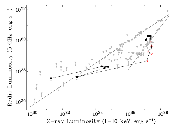
Figure 7: Correlation between the radio and X-ray luminosity during the outburst of MAXI J1659$-$152, compared to other BHXBs (grey symbols). The grey lines indicate the two tracks in the radio-X-ray correlation with slopes of $\sim 0.7$ and $\sim 1.4$. The MAXI J1659$-$152 luminosities are calculated for a source distance of 6 kpc. The black solid circles indicate the early times of the outburst when the radio emission in MAXI J1659$-$152 had not dropped significantly yet (up to day 8 after the outburst onset) and the late times when the source is almost in quiescence ($>135$ days), while the red open circles indicate the times in between.

In Section 4.1 we have discussed the related behavior between the radio and X-ray regime for MAXI J1659$-$152, and the implied link between the accretion flow and the jet. We explore this further by investigating the correlation between the radio and X-ray luminosities throughout the outburst. This correlation was originally suggested for GX 339$-$4 when it was in the hard state (Hannikainen et al., 1998) and described by a power law with index $\sim 0.7$ extending 3 orders of magnitude in luminosity with a turnover at high X-ray luminosities caused by a quenching of the radio emission in the soft state (Corbel et al., 2003; Gallo, Fender & Pooley, 2003). This correlation has not only been found and studied in detail for individual sources (e.g. Corbel, Koerding & Kaaret, 2008; Corbel et al., 2013b), but also for the sample of BHXBs as a whole (e.g. Gallo, Fender & Pooley, 2003). In recent years a more complex picture has revealed itself, with two distinct tracks in the radio/X-ray luminosity plane (e.g. Coriat et al., 2011; Gallo, Miller & Fender, 2012). The second track lies below the first one and has a steeper power-law index of $\sim 1.4$. For a few sources it has been shown that there is a transition from the lower to the upper track at low luminosities (Coriat et al., 2011; Ratti et al., 2012).

Figure 7 shows the correlation for MAXI J1659$-$152, and a comparison with other BHXBs in the hard state. Besides the radio observations presented in this paper, we included the late-time data from Jonker et al. (2012). The latter paper focused mainly on the late-time evolution when the source was close to quiescence and also showed the early radio fluxes that had been reported in the literature (van der Horst et al., 2010b; Paragi et al., 2010). To calculate the luminosities we adopted a distance to MAXI J1659$-$152 of 6 kpc, since the distances estimated in various ways span a range from 4 to 8 kpc (Kennea et al., 2011; Miller-Jones et al., 2011; Kaur et al., 2012; Kuulkers et al., 2013).

As shown by Jonker et al. (2012), MAXI J1659$-$152 was on the lower track early in the outburst, and once the source had reached quiescent levels, it seemed to transition to the upper track, although we note that the lowest-luminosity points have only radio upper limits. With our extensive data set during the early phases of the outburst we show in Figure 7 that the source gradually evolved off the correlation during the HIMS over the course of several days, as seen before in GX 339-4 (Corbel et al., 2013a) and expected for sources which are not in the hard state. However, the motion in the radio/X-ray plane was not monotonic during this radio quenching, with the radio emission fading and recovering between days 6 and 20, due in part to the repeated transitions between the HIMS and the SIMS.

5.2 Optical versus X-rays

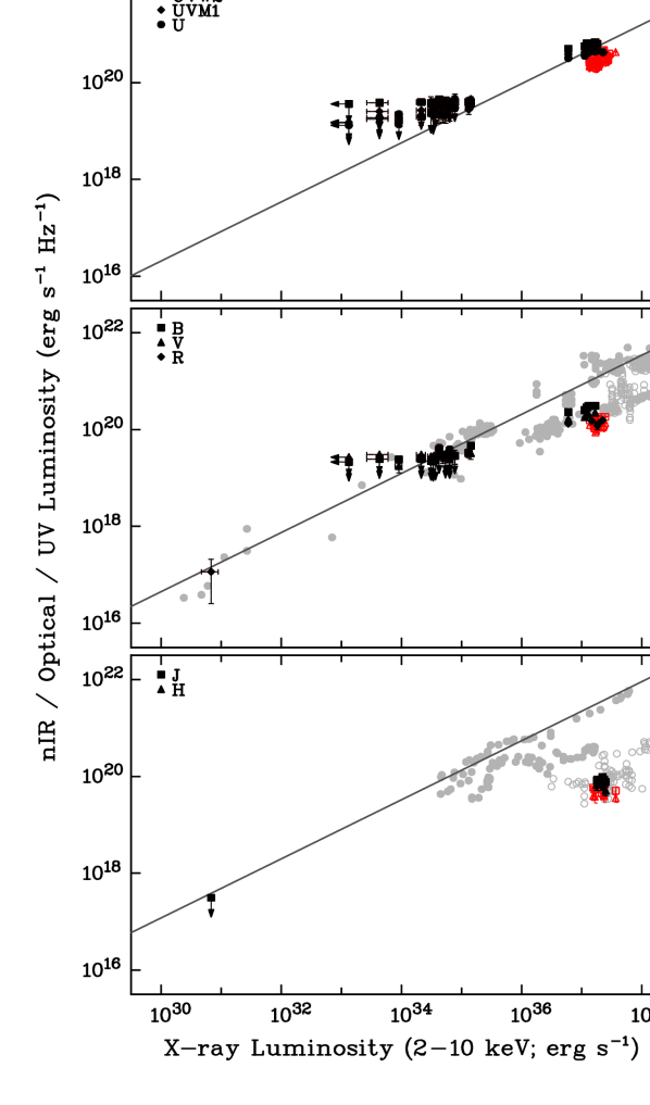
Figure 8: Correlation between the nIR/optical/UV and X-ray luminosity during the outburst of MAXI J1659$-$152. The MAXI J1659$-$152 luminosities are calculated for a source distance of 6 kpc. The black solid symbols indicate the early times of the outburst when the radio emission in MAXI J1659$-$152 had not dropped yet (up to day 8 after the outburst onset) and the late times when the source is almost in or in quiescence ($>135$ days), while the red open symbols indicate the times in between. The light grey symbols are for other BHXBs during the hard state (solid symbols) and soft state (open symbols) as presented by Russell et al. (2006) and Russell et al. (2007). The solid lines show the best-fit hard state nIR/optical-X-ray correlation from Russell et al. (2006).

While the radio emission is produced in the jet and the X-ray emission in the accretion disk and/or the corona, the nature of the UV, optical and nIR emission is less unambiguous. Most likely the UV emission is also produced in the accretion disk, either intrinsically or by reprocessing of X-rays, but in the optical and nIR there may also be a contribution from the jet. In Section 4.1 we have modeled the full SED from radio to X-ray frequencies with a combination of a broken power law and a physically motivated irradiated disk model. From these spectral fits we have concluded that a jet contribution at nIR wavelengths is not necessary. This conclusion, however, is model dependent and here we look deeper into this issue by investigating the correlations between the X-ray emission and the nIR, optical and UV emission.

A correlation between the nIR/optical and X-ray luminosity was first found for GX 339$-$4 in the hard state by Homan et al. (2005), with a power-law slope of $\sim 0.5$. Russell et al. (2006) has shown for a large sample of BHXBs in the hard state that there is such a correlation with a power-law slope of $\sim 0.6$ over eight orders of magnitude in X-ray luminosity. A correlation with such a power-law slope can be expected both in the case of X-ray reprocessing (van Paradijs & McClintock, 1994) and jet emission at nIR/optical wavelengths. Russell et al. (2006) have also shown that when these sources are in a soft state, the nIR and, in some cases, the optical emission is significantly suppressed. In Figure 8 we show the correlation between the UV/optical/nIR and X-ray luminosities for MAXI J1659$-$152. Similar to Figure 7 we have made a distinction between the early outburst before the radio emission strongly decreases (day 8 after the outburst onset; black solid symbols), the second phase of the outburst (red open symbols), and the very late times when the source has reached significantly lower luminosities in the radio, optical and X-rays (black solid symbols). We have also included the optical/nIR detections when the source is in quiescence, using the r-band magnitude at $\sim 1.5$ years after the outburst onset from Kong (2012), the J-band magnitude at $\sim 2.9$ years from this paper, and the quiescent X-ray flux at $\sim 1.8$ years reported in Homan et al. (2013). From the late-time magnitudes we have subtracted a contribution from the companion star of the black hole. It has been proposed (Kuulkers et al., 2013; Kong, 2012) that this is an M2 or M5 dwarf star, which have an absolute V-band magnitude of 10 and 11.8, respectively (Kong, 2012). We have converted these absolute magnitudes to apparent magnitudes in the r- and J-band by correcting for the typical color of these dwarf stars (Johnson, 1965) and galactic extinction, and by adopting a source distance of 6 kpc. The resulting r-band magnitude of the companion star is 24.3 (M2) or 25.8 (M5), and in the J-band it is 21.1 (M2) or 22.0 (M5). We have corrected the very-late time fluxes for these ranges in magnitudes, resulting in the large uncertainties displayed in Figure 8.

For comparison we plot in Figure 8 the optical/nIR-X-ray relations for the samples presented in Russell et al. (2006) and Russell et al. (2007), although here we show the luminosity divided by observing frequency for optical/nIR frequencies, i.e. the measured flux scaled by the source distance. For the other BHXBs the solid symbols indicate when they are in a hard state, while the open symbols are for the soft state. The top panel of Figure 8 shows that the UV emission is consistent with the hard state optical-X-ray correlation (Russell et al., 2006) throughout the outburst. In the middle panel it can be seen that MAXI J1659$-$152 resides in the same region of the correlation as several other hard state BHXBs in the optical, both early in the outburst before the radio emission is quenched and the late times when the source is going towards or is in quiescence. The data corresponding to times after the quenching of the radio emission lay below the correlation of hard state BHXBs, but they are consistent with other sources in the soft state. The bottom panel displays different behavior at nIR wavelengths: the data are well below the correlation for other hard state sources throughout the main outburst (no late-time nIR observations are available), but consistent with some BHXBs in the soft state. This suggests that at the time of our observations there is no significant contribution of the jet to the nIR emission, which is consistent with our conclusions from the broadband modeling in Section 4.1. Given the detection of a spectral break at radio frequencies the lack of nIR jet emission is not surprising. We note, however, that our nIR observations started $\sim 4$ days after the outburst onset, and our earliest detection of a break was at $\sim 6$ days, so there is a possibility that the nIR jet emission quenched much earlier than at radio wavelengths. This is consistent with what has been found in other sources, namely that the nIR emission from the jet drops as soon as a source enters the HIMS (e.g. Homan et al., 2005; Coriat et al., 2009; Russell et al., 2010b) while the radio flux quenches later (e.g. Fender, Belloni & Gallo, 2004), caused by the jet spectral break shifting to lower frequencies.

6 Conclusions

In this paper we have presented the results of our observing campaign of MAXI J1659$-$152 across the electromagnetic spectrum, resulting in one of the richest broadband data sets of a BHXB outburst with observations at radio, sub-millimeter, nIR, optical, UV and X-ray frequencies, from 1 day up to 3 years after the outburst onset. We have modeled SEDs from radio to X-ray frequencies at several epochs with a broken power law plus a physical irradiated disk model, and we have presented the radio-X-ray and nIR/optical/UV-X-ray correlations for MAXI J1659$-$152 in the context of other BHXBs.

We have found changes in the radio brightness and spectrum which are correlated with X-ray state changes, suggesting a link between the radio jet and the accretion flow that is dominating the X-ray emission. We have shown this based on our broadband SED modeling and by investigating the correlation between radio and X-ray luminosity. During the first weeks after the outburst onset MAXI J1659$-$152 moved away from the hard state into intermediate X-ray spectral states, based on spectral and timing behavior at X-ray energies. This was further evidenced by (1) the increasing disk temperature, steepening photon index and decreasing disk inner radius we have found in our SED modeling, (2) the quenching of the radio emission coming from the jet, and (3) the deviations from the radio-X-ray and nIR/optical/UV-X-ray correlations of BHXBs in the hard state.

The broadband radio light curves and spectra support the conclusions from Paragi et al. (2013), based on VLBI observations, that there was no major ejection event. Our radio observations also show the presence of a variable spectral break at radio frequencies during the HIMS and SIMS, significantly lower in frequency than typically found in hard state BHXBs. We have investigated the nIR/optical/UV-X-ray correlations and concluded that there is no significant contribution from the jet at nIR wavelengths, consistent with our broadband modeling. Taken with the results of Russell et al. (2013b) and Corbel et al. (2013a), this suggests that the spectral break, which lies at infrared frequencies during the hard state, evolves down in frequency during the HIMS and SIMS until it passes through the radio band.

Our findings for MAXI J1659$-$152 demonstrate that broadband observations covering several radio and nIR/optical/UV frequencies at a high cadence during BHXB outbursts are important for a better understanding of the jet and disk in these sources. On top of these observations, denser sampling at sub-millimeter and mid-infrared frequencies are crucial to accurately determine the evolution of the spectral break and further our understanding of the jet physics in these systems.

Table 2: UV, optical and nIR observations

Epoch (MJD)	Telescope	Filter	Magnitude
55468.050	SMARTS	H	14.70$\pm$0.13
55468.995	SMARTS	H	14.85$\pm$0.12
55469.999	SMARTS	H	14.88$\pm$0.21
55470.990	SMARTS	H	14.90$\pm$0.18
55472.002	SMARTS	H	15.02$\pm$0.08
55472.985	SMARTS	H	15.22$\pm$0.15
55476.002	SMARTS	H	15.33$\pm$0.14
55476.994	SMARTS	H	15.60$\pm$0.14
55478.010	SMARTS	H	15.40$\pm$0.14
55478.997	SMARTS	H	15.50$\pm$0.18
55479.997	SMARTS	H	15.49$\pm$0.14
55481.006	SMARTS	H	15.54$\pm$0.24
55483.002	SMARTS	H	15.51$\pm$0.21
55468.044	SMARTS	J	15.13$\pm$0.13
55468.990	SMARTS	J	15.27$\pm$0.19
55469.993	SMARTS	J	15.26$\pm$0.10
55470.984	SMARTS	J	15.32$\pm$0.21
55471.996	SMARTS	J	15.26$\pm$0.16
55472.979	SMARTS	J	15.41$\pm$0.23
55475.996	SMARTS	J	15.52$\pm$0.11
55476.988	SMARTS	J	15.84$\pm$0.21
55478.004	SMARTS	J	15.68$\pm$0.11
55478.991	SMARTS	J	15.76$\pm$0.10
55479.991	SMARTS	J	15.70$\pm$0.10
55481.001	SMARTS	J	15.83$\pm$0.10
55482.997	SMARTS	J	15.79$\pm$0.06
56497.977	3.5m CAHA	J	21.05$\pm$0.17
55710.964	2.2m CAHA	z	18.45$\pm$0.10
55464.836	IAC80	I	16.09$\pm$0.05
55486.768	1.23m CAHA	I	16.59$\pm$0.08
55641.198	1.23m CAHA	I	17.95$\pm$0.23
55685.141	2.0m LT	i	19.87$\pm$0.05
55708.960	2.2m CAHA	i	18.72$\pm$0.05
55709.981	2.2m CAHA	i	18.77$\pm$0.09
55710.041	2.2m CAHA	i	18.59$\pm$0.15
55710.958	2.2m CAHA	i	18.79$\pm$0.06
55464.826	IAC80	R	16.59$\pm$0.06
55464.834	IAC80	R	16.61$\pm$0.05
55464.838	BOOTES-2	R	16.59$\pm$0.09
55464.838	IAC80	R	16.58$\pm$0.06
55464.839	IAC80	R	16.62$\pm$0.05
55464.840	IAC80	R	16.59$\pm$0.06
55464.840	IAC80	R	16.56$\pm$0.06
55464.841	IAC80	R	16.58$\pm$0.06
55464.841	IAC80	R	16.56$\pm$0.06
55464.842	IAC80	R	16.59$\pm$0.06
55464.842	IAC80	R	16.57$\pm$0.06
55464.843	IAC80	R	16.55$\pm$0.06
55464.843	IAC80	R	16.56$\pm$0.07
55464.846	IAC80	R	16.57$\pm$0.07
55464.849	IAC80	R	16.54$\pm$0.07
55466.799	BOOTES-2	R	16.45$\pm$0.07
55468.798	BOOTES-2	R	16.41$\pm$0.06
55469.790	BOOTES-2	R	16.59$\pm$0.06
55641.195	1.23m CAHA	R	18.57$\pm$0.21
55470.793	BOOTES-2	r	16.69$\pm$0.20
55474.358	BOOTES-3	r	16.78$\pm$0.11

Table 3: continued

UV, optical and nIR observations Epoch (MJD) Telescope Filter Magnitude 55474.383 BOOTES-3 r 16.74$\pm$0.11 55475.314 BOOTES-3 r 17.01$\pm$0.11 55475.336 BOOTES-3 r 17.02$\pm$0.11 55475.357 BOOTES-3 r 16.98$\pm$0.11 55475.378 BOOTES-3 r 16.95$\pm$0.11 55475.399 BOOTES-3 r 16.84$\pm$0.11 55708.960 2.2m CAHA r 19.03$\pm$0.04 55709.981 2.2m CAHA r 19.09$\pm$0.04 55710.041 2.2m CAHA r 19.15$\pm$0.12 55710.961 2.2m CAHA r 19.05$\pm$0.05 55464.627 UVOT V 16.775$\pm$0.032 55464.832 IAC80 V 16.94$\pm$0.03 55465.258 UVOT V 16.676$\pm$0.032 55465.735 UVOT V 16.571$\pm$0.038 55466.303 UVOT V 16.525$\pm$0.031 55467.635 UVOT V 16.450$\pm$0.036 55482.813 UVOT V 17.197$\pm$0.083 55483.489 UVOT V 17.171$\pm$0.067 55484.025 UVOT V 17.211$\pm$0.080 55485.028 UVOT V 16.974$\pm$0.068 55486.031 UVOT V 17.046$\pm$0.068 55487.036 UVOT V 17.441$\pm$0.096 55488.040 UVOT V 17.178$\pm$0.079 55489.044 UVOT V 17.082$\pm$0.075 55490.042 UVOT V 17.337$\pm$0.107 55491.045 UVOT V 17.258$\pm$0.092 55598.791 UVOT V 18.576$\pm$0.284 55620.663 UVOT V $>$18.588 55634.878 UVOT V 18.756$\pm$0.303 55641.195 1.23m CAHA V 18.67$\pm$0.21 55647.369 UVOT V $>$18.963 55669.437 UVOT V $>$18.798 55687.980 UVOT V 19.253$\pm$0.298 55702.627 UVOT V 18.562$\pm$0.214 55717.735 UVOT V $>$18.662 55721.224 UVOT V $>$18.642 55725.361 UVOT V $>$18.661 55729.780 UVOT V $>$18.622 55733.057 UVOT V $>$18.625 55737.405 UVOT V $>$18.788 55741.027 UVOT V $>$18.745 55745.765 UVOT V $>$18.648 55749.584 UVOT V $>$18.658 55757.421 UVOT V $>$18.610 55759.752 UVOT V $>$18.554 55761.296 UVOT V $>$18.344 55470.793 BOOTES-2 g 17.31$\pm$0.15 55476.785 BOOTES-2 g 17.42$\pm$0.17 55708.960 2.2m CAHA g 19.60$\pm$0.07 55709.981 2.2m CAHA g 19.66$\pm$0.05 55710.041 2.2m CAHA g 19.81$\pm$0.19 55710.961 2.2m CAHA g 19.62$\pm$0.07 55464.666 UVOT B 17.114$\pm$0.023 55464.830 IAC80 B 17.38$\pm$0.07 55465.334 UVOT B 17.014$\pm$0.026 55465.727 UVOT B 16.883$\pm$0.028 55466.291 UVOT B 16.818$\pm$0.023

Table 4: continued

UV, optical and nIR observations Epoch (MJD) Telescope Filter Magnitude 55466.628 UVOT B 16.804$\pm$0.030 55467.629 UVOT B 16.795$\pm$0.027 55482.823 UVOT B 17.378$\pm$0.046 55483.502 UVOT B 17.529$\pm$0.045 55484.035 UVOT B 17.482$\pm$0.049 55485.038 UVOT B 17.366$\pm$0.046 55486.042 UVOT B 17.460$\pm$0.048 55487.046 UVOT B 17.761$\pm$0.061 55488.050 UVOT B 17.483$\pm$0.050 55489.054 UVOT B 17.538$\pm$0.053 55490.050 UVOT B 17.769$\pm$0.072 55491.055 UVOT B 17.613$\pm$0.059 55598.851 UVOT B 18.908$\pm$0.128 55620.657 UVOT B 19.183$\pm$0.288 55634.872 UVOT B 19.434$\pm$0.240 55641.198 1.23m CAHA B 19.71$\pm$0.48 55647.363 UVOT B 19.507$\pm$0.252 55669.431 UVOT B $>$19.745 55687.975 UVOT B 19.624$\pm$0.177 55702.620 UVOT B 19.281$\pm$0.176 55717.730 UVOT B $>$19.600 55721.219 UVOT B 19.440$\pm$0.342 55725.356 UVOT B $>$19.607 55729.775 UVOT B 19.073$\pm$0.256 55733.052 UVOT B $>$19.585 55737.399 UVOT B $>$19.738 55741.021 UVOT B $>$19.702 55745.760 UVOT B $>$19.605 55749.579 UVOT B $>$19.595 55757.483 UVOT B $>$19.963 55759.748 UVOT B $>$19.512 55761.428 UVOT B $>$19.893 55464.662 UVOT U 16.144$\pm$0.025 55465.267 UVOT U 16.036$\pm$0.025 55465.725 UVOT U 15.905$\pm$0.028 55466.288 UVOT U 15.845$\pm$0.025 55466.625 UVOT U 15.787$\pm$0.059 55467.628 UVOT U 15.816$\pm$0.027 55468.494 UVOT U 15.840$\pm$0.025 55482.819 UVOT U 16.450$\pm$0.037 55483.496 UVOT U 16.468$\pm$0.034 55484.030 UVOT U 16.565$\pm$0.039 55485.033 UVOT U 16.382$\pm$0.036 55486.037 UVOT U 16.510$\pm$0.037 55487.041 UVOT U 16.698$\pm$0.041 55488.046 UVOT U 16.550$\pm$0.039 55489.049 UVOT U 16.591$\pm$0.040 55490.046 UVOT U 16.725$\pm$0.047 55491.050 UVOT U 16.678$\pm$0.042 55598.850 UVOT U 18.624$\pm$0.132 55620.656 UVOT U 18.498$\pm$0.215 55634.871 UVOT U 18.469$\pm$0.146 55647.362 UVOT U 19.112$\pm$0.244 55669.629 UVOT U $>$19.660 55687.974 UVOT U 19.078$\pm$0.151 55702.619 UVOT U 18.715$\pm$0.149 55717.729 UVOT U 18.770$\pm$0.265

Table 5: continued

UV, optical and nIR observations Epoch (MJD) Telescope Filter Magnitude 55721.218 UVOT U 18.762$\pm$0.268 55725.355 UVOT U 18.685$\pm$0.242 55729.774 UVOT U 19.125$\pm$0.356 55733.051 UVOT U 19.132$\pm$0.351 55737.397 UVOT U 18.896$\pm$0.263 55741.020 UVOT U 18.591$\pm$0.216 55745.759 UVOT U 19.184$\pm$0.375 55749.578 UVOT U $>$19.275 55757.482 UVOT U $>$19.635 55759.747 UVOT U $>$19.202 55761.427 UVOT U $>$19.567 55708.960 2.2m CAHA u 19.81$\pm$0.05 55709.981 2.2m CAHA u 19.83$\pm$0.07 55710.041 2.2m CAHA u 19.66$\pm$0.17 55710.961 2.2m CAHA u 20.04$\pm$0.28 55464.656 UVOT UVW1 16.438$\pm$0.024 55465.260 UVOT UVW1 16.307$\pm$0.024 55465.723 UVOT UVW1 16.196$\pm$0.027 55466.284 UVOT UVW1 16.117$\pm$0.024 55467.626 UVOT UVW1 16.103$\pm$0.026 55471.384 UVOT UVW1 16.240$\pm$0.025 55472.120 UVOT UVW1 16.317$\pm$0.027 55475.400 UVOT UVW1 16.505$\pm$0.025 55476.128 UVOT UVW1 16.483$\pm$0.029 55476.664 UVOT UVW1 16.528$\pm$0.029 55479.073 UVOT UVW1 16.697$\pm$0.035 55479.541 UVOT UVW1 16.723$\pm$0.031 55482.891 UVOT UVW1 16.639$\pm$0.047 55484.576 UVOT UVW1 16.848$\pm$0.052 55485.505 UVOT UVW1 16.823$\pm$0.053 55488.578 UVOT UVW1 16.765$\pm$0.054 55489.527 UVOT UVW1 16.993$\pm$0.063 55490.586 UVOT UVW1 17.112$\pm$0.070 55491.257 UVOT UVW1 17.165$\pm$0.071 55598.848 UVOT UVW1 18.844$\pm$0.120 55620.654 UVOT UVW1 19.022$\pm$0.257 55634.869 UVOT UVW1 19.459$\pm$0.251 55647.361 UVOT UVW1 19.150$\pm$0.208 55669.628 UVOT UVW1 $>$20.034 55687.973 UVOT UVW1 19.722$\pm$0.204 55702.616 UVOT UVW1 19.395$\pm$0.211 55717.727 UVOT UVW1 19.349$\pm$0.341 55721.216 UVOT UVW1 18.815$\pm$0.235 55725.353 UVOT UVW1 19.126$\pm$0.284 55729.773 UVOT UVW1 19.286$\pm$0.325 55733.050 UVOT UVW1 19.360$\pm$0.353 55737.396 UVOT UVW1 $>$19.658 55741.019 UVOT UVW1 $>$19.614 55745.758 UVOT UVW1 $>$19.419 55749.577 UVOT UVW1 $>$19.490 55757.481 UVOT UVW1 $>$19.905 55759.746 UVOT UVW1 $>$19.412 55761.426 UVOT UVW1 $>$19.846 55464.623 UVOT UVW2 16.548$\pm$0.028 55465.324 UVOT UVW2 16.470$\pm$0.028 55465.732 UVOT UVW2 16.326$\pm$0.025 55466.297 UVOT UVW2 16.251$\pm$0.023

Table 6: continued

UV, optical and nIR observations Epoch (MJD) Telescope Filter Magnitude 55467.632 UVOT UVW2 16.245$\pm$0.024 55469.478 UVOT UVW2 16.399$\pm$0.026 55473.392 UVOT UVW2 16.506$\pm$0.025 55477.132 UVOT UVW2 16.602$\pm$0.030 55477.668 UVOT UVW2 16.819$\pm$0.031 55482.880 UVOT UVW2 16.853$\pm$0.050 55484.565 UVOT UVW2 17.014$\pm$0.052 55485.494 UVOT UVW2 17.094$\pm$0.055 55488.569 UVOT UVW2 17.111$\pm$0.057 55489.519 UVOT UVW2 17.095$\pm$0.060 55490.579 UVOT UVW2 17.366$\pm$0.072 55491.249 UVOT UVW2 17.348$\pm$0.069 55598.852 UVOT UVW2 19.249$\pm$0.100 55620.660 UVOT UVW2 19.859$\pm$0.302 55634.875 UVOT UVW2 19.889$\pm$0.214 55647.366 UVOT UVW2 19.751$\pm$0.201 55669.434 UVOT UVW2 $>$20.301 55687.977 UVOT UVW2 20.305$\pm$0.201 55702.624 UVOT UVW2 19.505$\pm$0.143 55717.732 UVOT UVW2 19.880$\pm$0.310 55721.222 UVOT UVW2 19.441$\pm$0.231 55725.358 UVOT UVW2 19.291$\pm$0.201 55729.778 UVOT UVW2 19.463$\pm$0.232 55733.055 UVOT UVW2 19.332$\pm$0.216 55737.402 UVOT UVW2 19.624$\pm$0.235 55741.024 UVOT UVW2 19.672$\pm$0.250 55745.763 UVOT UVW2 19.993$\pm$0.344 55749.582 UVOT UVW2 $>$20.115 55757.484 UVOT UVW2 $>$20.230 55759.750 UVOT UVW2 $>$20.005 55761.430 UVOT UVW2 $>$20.298 55464.633 UVOT UVM2 16.950$\pm$0.033 55465.250 UVOT UVM2 16.835$\pm$0.029 55465.739 UVOT UVM2 16.687$\pm$0.032 55466.270 UVOT UVM2 16.683$\pm$0.033 55467.638 UVOT UVM2 16.602$\pm$0.032 55470.481 UVOT UVM2 16.702$\pm$0.031 55474.362 UVOT UVM2 17.023$\pm$0.032 55478.136 UVOT UVM2 17.174$\pm$0.042 55478.671 UVOT UVM2 17.202$\pm$0.042 55482.886 UVOT UVM2 17.228$\pm$0.072 55484.571 UVOT UVM2 17.435$\pm$0.077 55485.500 UVOT UVM2 17.519$\pm$0.082 55488.574 UVOT UVM2 17.511$\pm$0.084 55489.523 UVOT UVM2 17.451$\pm$0.087 55490.583 UVOT UVM2 17.760$\pm$0.107 55491.253 UVOT UVM2 17.674$\pm$0.100 55598.794 UVOT UVM2 19.738$\pm$0.296 55620.666 UVOT UVM2 $>$19.757 55634.880 UVOT UVM2 20.274$\pm$0.374 55647.370 UVOT UVM2 $>$20.039 55669.440 UVOT UVM2 $>$19.817 55687.982 UVOT UVM2 $>$20.656 55702.630 UVOT UVM2 19.713$\pm$0.240 55717.737 UVOT UVM2 $>$19.584 55721.226 UVOT UVM2 $>$19.728 55725.363 UVOT UVM2 $>$19.763

Table 7: continued

UV, optical and nIR observations Epoch (MJD) Telescope Filter Magnitude 55729.782 UVOT UVM2 $>$19.587 55733.059 UVOT UVM2 $>$19.648 55737.407 UVOT UVM2 $>$19.720 55741.029 UVOT UVM2 19.780$\pm$0.369 55745.767 UVOT UVM2 $>$19.724 55749.586 UVOT UVM2 $>$19.752 55757.423 UVOT UVM2 $>$19.720 55759.754 UVOT UVM2 $>$19.625 55761.298 UVOT UVM2 $>$19.405

References

- Belloni (2010) Belloni T., ed., 2010, Lecture Notes in Physics, Berlin Springer Verlag, Vol. 794, The Jet Paradigm
- Belloni, Motta & Muñoz-Darias (2010) Belloni T. M., Motta S., Muñoz-Darias T., 2010, The Astronomer’s Telegram, 2927, 1
- Belloni, Muñoz-Darias & Kuulkers (2010) Belloni T. M., Muñoz-Darias T., Kuulkers E., 2010, The Astronomer’s Telegram, 2926, 1
- Breeveld et al. (2010) Breeveld A. A. et al., 2010, MNRAS, 406, 1687
- Casella, Belloni & Stella (2005) Casella P., Belloni T., Stella L., 2005, ApJ, 629, 403
- Castro-Tirado et al. (1999) Castro-Tirado A. J. et al., 1999, A&AS, 138, 583
- Corbel et al. (2013a) Corbel S. et al., 2013a, MNRAS, 431, L107
- Corbel et al. (2013b) Corbel S., Coriat M., Brocksopp C., Tzioumis A. K., Fender R. P., Tomsick J. A., Buxton M. M., Bailyn C. D., 2013b, MNRAS, 428, 2500
- Corbel & Fender (2002) Corbel S., Fender R. P., 2002, ApJ, 573, L35
- Corbel, Koerding & Kaaret (2008) Corbel S., Koerding E., Kaaret P., 2008, MNRAS, 389, 1697
- Corbel et al. (2003) Corbel S., Nowak M. A., Fender R. P., Tzioumis A. K., Markoff S., 2003, A&A, 400, 1007
- Coriat et al. (2009) Coriat M., Corbel S., Buxton M. M., Bailyn C. D., Tomsick J. A., Körding E., Kalemci E., 2009, MNRAS, 400, 123
- Coriat et al. (2011) Coriat M. et al., 2011, MNRAS, 414, 677
- de Ugarte Postigo et al. (2010a) de Ugarte Postigo A., Flores H., Wiersema K., Thoene C. C., Fynbo J. P. U., Goldoni P., 2010a, GRB Coordinates Network, Circular Service, 11307, 1 (2010), 1307, 1
- de Ugarte Postigo et al. (2010b) de Ugarte Postigo A., Lundrgren A., Wyrowski F., Thoene C. C., Castro-Tirado A. J., Gorosabel J., Jelinek M., 2010b, GRB Coordinates Network, Circular Service, 11304, 1 (2010), 1304, 1
- Evans et al. (2009) Evans P. A. et al., 2009, MNRAS, 397, 1177
- Fender (2010) Fender R., 2010, in Lecture Notes in Physics, Berlin Springer Verlag, Vol. 794, Lecture Notes in Physics, Berlin Springer Verlag, Belloni T., ed., p. 115
- Fender (2001) Fender R. P., 2001, MNRAS, 322, 31
- Fender, Belloni & Gallo (2004) Fender R. P., Belloni T. M., Gallo E., 2004, MNRAS, 355, 1105
- Fender, Homan & Belloni (2009) Fender R. P., Homan J., Belloni T. M., 2009, MNRAS, 396, 1370
- Fukugita et al. (1996) Fukugita M., Ichikawa T., Gunn J. E., Doi M., Shimasaku K., Schneider D. P., 1996, AJ, 111, 1748
- Fukugita, Shimasaku & Ichikawa (1995) Fukugita M., Shimasaku K., Ichikawa T., 1995, PASP, 107, 945
- Gallo (2010) Gallo E., 2010, in Lecture Notes in Physics, Berlin Springer Verlag, Vol. 794, Lecture Notes in Physics, Berlin Springer Verlag, Belloni T., ed., p. 85
- Gallo, Fender & Pooley (2003) Gallo E., Fender R. P., Pooley G. G., 2003, MNRAS, 344, 60
- Gallo, Miller & Fender (2012) Gallo E., Miller B. P., Fender R., 2012, MNRAS, 423, 590
- Gandhi et al. (2011) Gandhi P. et al., 2011, ApJ, 740, L13
- Gierliński, Done & Page (2008) Gierliński M., Done C., Page K., 2008, MNRAS, 388, 753
- Gierliński, Done & Page (2009) Gierliński M., Done C., Page K., 2009, MNRAS, 392, 1106
- Gilfanov (2010) Gilfanov M., 2010, in Lecture Notes in Physics, Berlin Springer Verlag, Vol. 794, Lecture Notes in Physics, Berlin Springer Verlag, Belloni T., ed., p. 17
- Hannikainen et al. (1998) Hannikainen D. C., Hunstead R. W., Campbell-Wilson D., Sood R. K., 1998, A&A, 337, 460
- Homan & Belloni (2005) Homan J., Belloni T., 2005, Ap&SS, 300, 107
- Homan et al. (2005) Homan J., Buxton M., Markoff S., Bailyn C. D., Nespoli E., Belloni T., 2005, ApJ, 624, 295
- Homan et al. (2013) Homan J., Fridriksson J. K., Jonker P. G., Russell D. M., Gallo E., Kuulkers E., Rea N., Altamirano D., 2013, ArXiv e-prints
- Homan et al. (2001) Homan J., Wijnands R., van der Klis M., Belloni T., van Paradijs J., Klein-Wolt M., Fender R., Méndez M., 2001, ApJS, 132, 377
- Jelinek et al. (2010) Jelinek M. et al., 2010, GRB Coordinates Network, Circular Service, 11301, 1 (2010), 1301, 1
- Johnson (1965) Johnson H. L., 1965, ApJ, 141, 170
- Jonker et al. (2012) Jonker P. G., Miller-Jones J. C. A., Homan J., Tomsick J., Fender R. P., Kaaret P., Markoff S., Gallo E., 2012, MNRAS, 423, 3308
- Jordi, Grebel & Ammon (2006) Jordi K., Grebel E. K., Ammon K., 2006, A&A, 460, 339
- Kalamkar et al. (2011) Kalamkar M., Homan J., Altamirano D., van der Klis M., Casella P., Linares M., 2011, ApJ, 731, L2
- Kalamkar et al. (2010) Kalamkar M. et al., 2010, The Astronomer’s Telegram, 2881, 1
- Kalberla et al. (2005) Kalberla P. M. W., Burton W. B., Hartmann D., Arnal E. M., Bajaja E., Morras R., Pöppel W. G. L., 2005, A&A, 440, 775
- Kann (2010) Kann D. A., 2010, GRB Coordinates Network, Circular Service, 11299, 1 (2010), 1299, 1
- Kaur et al. (2012) Kaur R. et al., 2012, ApJ, 746, L23
- Kennea et al. (2010) Kennea J. A., Krimm H., Mangano V., Curran P., Romano P., Evans P., Burrows D. N., 2010, The Astronomer’s Telegram, 2877, 1
- Kennea et al. (2011) Kennea J. A. et al., 2011, ApJ, 736, 22
- Kong (2012) Kong A. K. H., 2012, ApJ, 760, L27
- Kuulkers et al. (1999) Kuulkers E., Fender R. P., Spencer R. E., Davis R. J., Morison I., 1999, MNRAS, 306, 919
- Kuulkers et al. (2010) Kuulkers E. et al., 2010, The Astronomer’s Telegram, 2912, 1
- Kuulkers et al. (2013) Kuulkers E. et al., 2013, A&A, 552, A32
- Kuulkers et al. (2012) Kuulkers E. et al., 2012, in The First Year of MAXI: Monitoring variable X-ray sources – 4th International MAXI Workshop, Mihara T. & Serino M., ed., Vol. IPCR CR-127, 81
- Lundgren et al. (2010) Lundgren A. et al., 2010, in Society of Photo-Optical Instrumentation Engineers (SPIE) Conference Series, Vol. 7737, Society of Photo-Optical Instrumentation Engineers (SPIE) Conference Series
- Malzac, Dumont & Mouchet (2005) Malzac J., Dumont A. M., Mouchet M., 2005, A&A, 430, 761
- Mangano et al. (2010) Mangano V., Hoversten E. A., Markwardt C. B., Sbarufatti B., Starling R. L. C., Ukwatta T. N., 2010, GRB Coordinates Network, Circular Service, 11296, 1 (2010), 1296, 1
- Markoff & Nowak (2004) Markoff S., Nowak M. A., 2004, ApJ, 609, 972
- Marshall (2010) Marshall F. E., 2010, GRB Coordinates Network, Circular Service, 11298, 1 (2010), 1298, 1
- McClintock & Remillard (2006) McClintock J. E., Remillard R. A., 2006, Black hole binaries, Lewin W. H. G., van der Klis M., eds., pp. 157–213
- Miller, Homan & Miniutti (2006) Miller J. M., Homan J., Miniutti G., 2006, ApJ, 652, L113
- Miller-Jones et al. (2011) Miller-Jones J. C. A., Madej O. K., Jonker P. G., Homan J., Ratti E. M., Torres M. A. P., 2011, The Astronomer’s Telegram, 3358, 1
- Miller-Jones et al. (2012) Miller-Jones J. C. A. et al., 2012, MNRAS, 421, 468
- Mirabel et al. (1992) Mirabel I. F., Rodriguez L. F., Cordier B., Paul J., Lebrun F., 1992, Nature, 358, 215
- Monet et al. (2003) Monet D. G. et al., 2003, AJ, 125, 984
- Motta et al. (2011) Motta S., Muñoz-Darias T., Casella P., Belloni T., Homan J., 2011, MNRAS, 418, 2292
- Muñoz-Darias et al. (2011) Muñoz-Darias T., Motta S., Stiele H., Belloni T. M., 2011, MNRAS, 415, 292
- Muñoz-Darias et al. (2010) Muñoz-Darias T., Stiele H., Belloni T. M., Motta S., 2010, The Astronomer’s Telegram, 2999, 1
- Negoro et al. (2010) Negoro H. et al., 2010, The Astronomer’s Telegram, 2873, 1
- Paragi et al. (2013) Paragi Z. et al., 2013, MNRAS, 432, 1319
- Paragi et al. (2010) Paragi Z. et al., 2010, The Astronomer’s Telegram, 2906, 1
- Poole et al. (2008) Poole T. S. et al., 2008, MNRAS, 383, 627
- Ratti et al. (2012) Ratti E. M. et al., 2012, MNRAS, 423, 2656
- Rushton et al. (2012) Rushton A. et al., 2012, MNRAS, 419, 3194
- Russell et al. (2006) Russell D. M., Fender R. P., Hynes R. I., Brocksopp C., Homan J., Jonker P. G., Buxton M. M., 2006, MNRAS, 371, 1334
- Russell et al. (2010a) Russell D. M. et al., 2010a, The Astronomer’s Telegram, 2884, 1
- Russell et al. (2007) Russell D. M., Maccarone T. J., Körding E. G., Homan J., 2007, MNRAS, 379, 1401
- Russell et al. (2010b) Russell D. M., Maitra D., Dunn R. J. H., Markoff S., 2010b, MNRAS, 405, 1759
- Russell et al. (2013a) Russell D. M. et al., 2013a, MNRAS, 429, 815
- Russell et al. (2013b) Russell D. M. et al., 2013b, ApJ, 768, L35
- Rykoff et al. (2007) Rykoff E. S., Miller J. M., Steeghs D., Torres M. A. P., 2007, ApJ, 666, 1129
- Sault, Teuben & Wright (1995) Sault R. J., Teuben P. J., Wright M. C. H., 1995, in Astronomical Society of the Pacific Conference Series, Vol. 77, Astronomical Data Analysis Software and Systems IV, Shaw R. A., Payne H. E., Hayes J. J. E., eds., p. 433
- Schlegel, Finkbeiner & Davis (1998) Schlegel D. J., Finkbeiner D. P., Davis M., 1998, ApJ, 500, 525
- Shakura & Sunyaev (1973) Shakura N. I., Sunyaev R. A., 1973, A&A, 24, 337
- Shaposhnikov & Yamaoka (2010) Shaposhnikov N., Yamaoka K., 2010, The Astronomer’s Telegram, 2951, 1
- Siringo et al. (2009) Siringo G. et al., 2009, A&A, 497, 945
- Skrutskie et al. (1995) Skrutskie M. F. et al., 1995, in Bulletin of the American Astronomical Society, Vol. 27, American Astronomical Society Meeting Abstracts, p. 1392
- Soria (2007) Soria R., 2007, Ap&SS, 311, 213
- Subasavage et al. (2010) Subasavage J. P., Bailyn C. D., Smith R. C., Henry T. J., Walter F. M., Buxton M. M., 2010, in Society of Photo-Optical Instrumentation Engineers (SPIE) Conference Series, Vol. 7737, Society of Photo-Optical Instrumentation Engineers (SPIE) Conference Series
- Tan (1991) Tan G. H., 1991, in Astronomical Society of the Pacific Conference Series, Vol. 19, IAU Colloq. 131: Radio Interferometry. Theory, Techniques, and Applications, Cornwell T. J., Perley R. A., eds., pp. 42–46
- van der Horst et al. (2010a) van der Horst A. J., Granot J., Paragi Z., Kouveliotou C., Wijers R. A. M. J., Ramirez-Ruiz E., 2010a, GRB Coordinates Network, Circular Service, 11309, 1 (2010), 1309, 1
- van der Horst et al. (2010b) van der Horst A. J., Granot J., Paragi Z., Kouveliotou C., Wijers R. A. M. J., Ramirez-Ruiz E., 2010b, The Astronomer’s Telegram, 2874, 1
- van der Horst et al. (2010c) van der Horst A. J. et al., 2010c, The Astronomer’s Telegram, 2918, 1
- van Paradijs & McClintock (1994) van Paradijs J., McClintock J. E., 1994, A&A, 290, 133
- Wells (1985) Wells D. C., 1985, in Data Analysis in Astronomy, di Gesu V., Scarsi L., Crane P., Friedman J. H., Levialdi S., eds., p. 195
- Wijnands, Homan & van der Klis (1999) Wijnands R., Homan J., van der Klis M., 1999, ApJ, 526, L33
- Wilson et al. (2011) Wilson W. E. et al., 2011, MNRAS, 416, 832
- Xu (2010) Xu D., 2010, GRB Coordinates Network, Circular Service, 11303, 1 (2010), 1303, 1
- Yamaoka et al. (2012) Yamaoka K. et al., 2012, PASJ, 64, 32