Dynamics of Desorption with Lateral Diffusion

Abstract

The dynamics of desorption from a submonolayer of adsorbed atoms or ions are significantly influenced by the absence or presence of lateral diffusion of the adsorbed particles. When diffusion is present, the adsorbate configuration is simultaneously changed by two distinct processes, proceeding in parallel: adsorption/desorption, which changes the total adsorbate coverage, and lateral diffusion, which is coverage conserving. Inspired by experimental results, we here study the effects of these competing processes by kinetic Monte Carlo simulations of a simple lattice-gas model. In order to untangle the various effects, we perform large-scale simulations, in which we monitor coverage, correlation length, and cluster-size distributions, as well as the behavior of representative individual clusters, during desorption. For each initial adsorbate configuration, we perform multiple, independent simulations, without and with diffusion, respectively. We find that, compared to desorption without diffusion, the coverage-conserving diffusion process produces two competing effects: a retardation of the desorption rate, which is associated with a coarsening of the adsorbate configuration, and an acceleration due to desorption of monomers “evaporated” from the cluster perimeters. The balance between these two effects is governed by the structure of the adsorbate layer at the beginning of the desorption process. Deceleration and coarsening are predominant for configurations dominated by monomers and small clusters, while acceleration is predominant for configurations dominated by large clusters.

I Introduction

Island growth and dissolution on surfaces are important non-equilibrium problems, both from fundamental and technological points of view. The interplay of adsorption, desorption, and lateral diffusion of adsorbate particles is essential to understanding cluster dynamics, and it has therefore been extensively studied.HON67 ; ABR70 ; GIL72 ; GIL76 ; BAR92 ; BAR93 ; BAR95 ; BAR96 ; MOR96 ; MOR99 ; LEH00 ; LEH01 ; HEY01 ; YAO02 ; WAT04 ; FRA05 ; FRA06 ; KOD06 ; ROO08 ; NGU08 ; JUW13 The present investigation is inspired by two experimental studies.

He and Borguet studied gold cluster formation and dissolution on Au(111) electrodes.HEY01 In these experiments, during a short positive potential pulse, the surface reconstructed and gold atoms were released onto the reconstructed surface, where they quickly nucleated and formed monolayer clusters. After the pulse, the reconstruction was lifted and gold atoms were reabsorbed in such a way that small clusters tended to decay quickly, while large clusters initially continued to grow before they also eventually decayed. Island stability in this experiment was studied by monitoring the cluster dissolution dynamics. The overall dissolution dynamics of the clusters was described by plotting the cluster coverage, i.e., the fraction of the surface covered by clusters, as a function of time.

Bartelt et al.BAR95 ; BAR96 made cluster-by-cluster in situ observations of the coarsening process by Ostwald ripening LIF61 in Si/Si(001) submonolayer systems. They wanted to understand how each cluster behaves in response to its surroundings. In this case, atoms detach from clusters, diffuse through the two-dimensional adsorbate gas surrounding the clusters, and eventually attach to other clusters, with net flow from smaller to larger clusters. In general we can expect that the behavior of each cluster depends on the detailed configuration of the surrounding clusters. BAR96

Another typical application is the experimental study of underpotential deposition (UPD), e.g., of Cu on electrodes of Au(111).ATA00 In UPD, a submonolayer of one metal is electrochemically adsorbed onto another in a range of electrode potentials more positive than that in which bulk deposition occurs.RIK98

A large body of work exists on the effects of diffusion on cluster growth and pattern formation in systems undergoing net adsorption,MEAK98 and for systems undergoing coarsening by lateral diffusion at constant coverage.LIF61 ; KHAR95 ; KHAR98 ; MILL99 ; KARA09 Much less is known for systems undergoing net desorption.KRUG05 ; FRA05 ; FRA06 ; IVAN10 In the present study we therefore investigate in a simple lattice-gas model the changes in cluster dynamics and cluster size distribution that occur during desorption in the presence of lateral diffusion as the initial cluster configuration is varied. The change in initial configuration would result in the change of the surrounding configurations of any particular cluster at a given coverage or time. In general, the behavior of each cluster depends on the detailed configuration of the surrounding clusters.BAR96 The simultaneous action of the nonconserved-order-parameter processes of adsorption and desorption and the conserved-order-parameter process of lateral adparticle diffusionLIF61 leads to a complex interplay between acceleration and deceleration of the overall desorption process, depending on the details of the local configurations. BAR92 ; BAR96 ; FRA05 ; FRA06

Using Kinetic Monte Carlo (KMC) simulation of a single-layer lattice-gas model, we consider the simultaneous adsorption, desorption, and lateral diffusion processes. Specifically, we employ the $n$-fold way rejection-free KMC algorithm, BOR75 ; NOV01 ; GIL72 ; GIL76 in which the simulation clock is updated after every accepted move. We consider two kinds of elementary moves: (1) an adsorption/desorption move, and (2) a single-atom diffusion move to a nearest-neighbor site. During the simulation, we sample the time development of the adsorbate coverage and correlation length. At certain coverages or times we also analyze the clusters using the Hoshen-Kopelman algorithm. HOS76 With this algorithm we are able to measure cluster size distributions and to tag specific clusters and follow their individual dynamics. The restriction to submonolayer configurations is consistent with the situation in the experiments reported in Refs. HEY01, ; BAR95, ; BAR96, . Some preliminary results of our study were previously presented in Ref. JUW13, .

The rest of this paper is organized as follows. The model, algorithm, and the measured quantities are introduced in Sec. II. We present the procedures to prepare the initial configurations in Sec. III. The results are presented in Sec. IV, and our conclusions are summarized in Sec. V.

II Model, Algorithm, and Measurements

II.1 Lattice-gas Model

The simplest kind of model for adsorption, desorption, and lateral diffusion on a surface is a lattice-gas model. We limit our study to submonolayer systems, so that each lattice site can be occupied by at most one atom. In this model, we define the occupancy number $c_{i}=1$ when site $i$ is occupied, and $c_{i}=0$ otherwise. Adsorption is the process of occupying an empty lattice site by a single particle, while desorption is the opposite. Diffusion consists in the random hopping of a single particle to an empty nearest-neighbor site. We work with square lattices with a total number of sites $V=L\times L$ and periodic boundary conditions. The total number of adsorbed particles is $N_{p}=\sum_{i=1}^{V}c_{i}$, and the coverage (or particle concentration) is defined as

$$\theta={N_{p}}/{V}\;.$$ (1)

II.2 Hamiltonian and Kinetic Monte Carlo Algorithm

The grand-canonical effective Hamiltonian of the lattice-gas model for our system is

$${\mathcal{H}}=-\phi\sum_{\langle i,j\rangle}c_{i}(t)c_{j}(t)-\mu\sum_{i}c_{i}(t)\;,$$ (2)

where $\phi>0$ is an attractive nearest-neighbor interaction constant, and $\mu$ is the electrochemical potential. Below the model’s critical temperature $T_{c}$, the value of the latter at coexistence between the low-coverage and high-coverage phases is $\mu_{0}=-2\phi$. The first sum in Eq. (2) runs over all nearest-neighbor pairs of sites, and the second sum runs over all sites. This lattice-gas Hamiltonian is equivalent to a nearest-neighbor Ising spin model, ISING and the adsorption, desorption, and nearest-neighbor diffusion processes can conveniently be discussed in Ising language, using single spin-flip and Kawasaki nearest-neighbor spin-exchange moves.

The simulations were performed for a $256\times 256$ square lattice. The temperature $T$ equals $0.8T_{c}$ with $T_{c}$ the exact critical temperature of the Ising lattice-gas model. ONS44 This temperature is low enough to avoid complications due to critical fluctuations, while it is high enough to obtain multidroplet configurations. RIK94 ; FRA06 The electrochemical potential and temperature are hereafter given in dimensionless units of the interaction constant $\phi$. (Boltzmann’s constant $k_{B}=1$.) The length unit is the lattice constant of the two-dimensional simulation lattice.

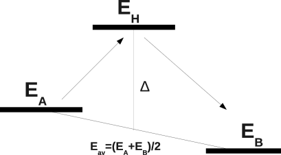
Figure 1: Energy barrier for transitions between states A and B. $E_{\rm H}$ is the maximum energy (saddle-point energy) along the transition path.

To obtain simulations that are closer to a real physical system, we consider the fact that when the system goes from a state of energy $E_{\rm A}$ to $E_{\rm B}$, it has to overcome an energy barrier (see Fig. 1). We define the height of the energy barrier ${\Delta}$ of the symmetric Butler-Volmer typeFRA06 as

$$\Delta = E_{\rm H}-\frac{1}{2}(E_{\rm A}+E_{\rm B})\;,$$ (3)

where $E_{\rm H}$ is the maximum energy (saddle-point energy) along the transition path. The energy difference between $E_{\rm H}$ and $E_{\rm A}$ is therefore

$$\Delta{\tilde{E}} = E_{\rm H}-E_{\rm A}$$ (4)

$$= \frac{1}{2}(E_{\rm B}-E_{\rm A})+\Delta.$$

Different processes have different barrier values: adsorption/desorption has barrier $\Delta_{\rm ads/des}$, and lateral diffusion has $\Delta_{\rm d}$. Since our objective is to study the competition between desorption and diffusion, for simplicity we use the same barrier $\Delta_{\rm d}$ for all diffusion moves, regardless of whether they occur along or away from a cluster edge.KHAR95 ; KHAR98 ; MILL99 ; YILD09 To study the effects of the diffusion on the desorption dynamics, we vary the difference $\left(\Delta_{\rm d}-\Delta_{\rm ads/des}\right)$. By keeping $\Delta_{\rm ads/des}$ constant and varying $\Delta_{\rm d}<\Delta_{\rm ads/des}$, we vary the ratio of the diffusion rate to the adsorption/desorption rate. The absolute values of the barriers have no particular meaning unless one attempts to specify the relation between physical and Monte Carlo time scales. In that case they would have to be calculated theoretically, for instance by quantum mechanical density functional theory (DFT),YILD09 ; JUWO11 or by comparison between simulations and experiments.BOTT96 ; ABOU04 In the present work, we treat the barriers as merely formal quantities.

A commonly used transition rate corresponding to Eq. (4) isFRA06

$$R_{\rm A\rightarrow\rm B}=\nu_{0}\exp\left(-\Delta/T\right)\exp\left[-(E_{\rm B}-E_{\rm A})/2T\right]\;,$$ (5)

where $\nu_{0}^{-1}$ determines the Monte Carlo time scale (one Monte Carlo Step per Site, MCSS), which is chosen as the basic time unit in the following. The above rate obeys detailed balance as the ratio $R_{A\rightarrow B}/R_{B\rightarrow A}$ cancels the prefactor, $\nu_{0}\exp\left(-\Delta/T\right)$.

The stochastic dynamics defined by this transition rate is here implemented by the continuous-time, rejection-free $n$-fold way Monte Carlo algorithm.BOR75 ; NOV01 ; GIL72 ; GIL76 This algorithm provides significant computational speed-up while preserving the underlying dynamics, at the expense of quite intricate programming. A detailed explanation of how the method is implemented in the model studied here is given in Ref. FRA06, .

II.3 Measurements

II.3.1 Morphology

One important measure closely related to the lateral diffusion is the correlation length. The correlation between the occupation at two sites $(i,j)~{}\mbox{and}~{}(i^{\prime},j^{\prime})$ is $c(i,j)c(i^{\prime},j^{\prime})$. (Here, the double indices, $i$ and $j$, refer to the two lattice directions.) With this expression, we define the correlation function $\Gamma(l)$, averaged over the two lattice directions, as

$$\Gamma(l)=\left(\frac{1}{L^{2}}\sum\limits_{i=1}^{L}\sum\limits_{j=1}^{L}c(i,j)\frac{c(i+l,j)+c(i,j+l)}{2}\right)-\left(\frac{1}{L^{2}}\sum\limits_{i=1}^{L}\sum\limits_{j=1}^{L}c(i,j)\right)^{2}\;,$$ (6)

where $0~{}\leq~{}l~{}\leq~{}L/2$. For $l=0$, Eq. (6) reduces to $\Gamma(0)=\theta(1-\theta)$, and the normalized correlation function is defined as $\gamma(l)={\Gamma(l)}/{\Gamma(0)}$. The correlation length $\xi$ is estimated from the inverse of the initial slope of the normalized correlation function $\gamma(l)$. For the discrete case of our lattice-gas model, this can be written asDEB57 ; JUW12

$$\xi=\frac{1}{1-\gamma(1)}\;.$$ (7)

Those lattice edges that connect an occupied and an empty lattice site are often called “broken bonds.” Their number, $\Sigma$, equals the total size of the interface between occupied and empty sites. It can be shown that $\xi$, as estimated by Eq. (7), is related to $\Sigma$ and $\theta$ asDEB57 ; BROW02 ; JUW12

$$\xi=\frac{4\theta(1-\theta)}{\Sigma/V}\;.$$ (8)

Other important average properties of the adsorbate configuration are the cluster number density $n_{s}$ and the Mean Cluster Size $S$. In introducing these quantities we closely follow the exposition and notation of Ref. STA92, . For $N_{s}$ clusters containing $s$ occupied sites each, the cluster number density,

$$n_{s}={N_{s}}/{V}\;,$$ (9)

is the number of such $s$-particle clusters per lattice site. Hence, the area density distribution, $n_{s}s$, is the probability that a randomly chosen site belongs to an $s$-cluster, and the coverage, $\theta=\sum\limits_{s}n_{s}s$, is the probability that it belongs to any cluster, i.e., that it is occupied. Thus, the probability that the cluster to which an arbitrary occupied site belongs contains exactly $s$ sites is $w_{s}={n_{s}s}/{\sum\limits_{s}n_{s}s}$. The mean cluster size $S$ that we measure in this process of randomly hitting some occupied site is therefore

$${S}=\sum\limits_{s}w_{s}s=\frac{\sum\limits_{s}n_{s}s^{2}}{\sum\limits_{s}n_{s}s}\;.$$ (10)

The magnitude of change of size distributions at a given coverage is measured by the changes in the mean cluster size $S$ and the cluster density,

$$\rho_{\delta}=\sum_{s}n_{s}\;,$$ (11)

which is the total number of clusters per unit area.

The details of the size distribution at the beginning of and during the desorption are obtained from number density ($n_{s}$) histogram plots,FRA05 each averaged over 100 independent runs. Therefore, $n_{s}$ becomes an estimate for the probability of finding the center of mass of a cluster of size $s$ at a randomly chosen site.FRA05 ; STA92 The number density for larger clusters is very low compared to that of the small clusters. For that reason we use exponentially growing bins for the histograms. The bins are set up such that each bin is twice as large as the previous one. This results in an uniform distribution of data points on a logarithmic scale.Norms

II.3.2 Dynamics

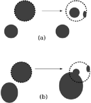
Figure 2: Cluster tagging. (a) A cluster shrinks and splits into two fragments. Here the larger of the two is taken as representative of the cluster. (b) A cluster shrinks and splits into two multi-atom fragments. One of these fragments coalesces with a larger cluster. The new coalesced cluster is then taken as representative of the split cluster.

The dynamics of the entire system is studied by measuring $\theta(t)$, while the individual cluster dynamics are observed by tagging a specific cluster at the beginning of the desorption process, and following it while measuring its size as a function of time, $s_{i}(t)$, during the whole process. Figure 2 illustrates our cluster-tagging procedure. We pick a specific cluster at the beginning of the desorption simulation and record the coordinates of all the points in the cluster. During the simulation process we monitor those coordinates. We record the cluster labels at each of those coordinates at any given time and obtain the cluster size as a function of time. Figure 2(a) gives an example in which the cluster shrinks and splits into two fragments. In this case we take the largest cluster within the circle as the representative of the cluster. There is also a possibility that the cluster just splits into two fragments of comparable sizes. In this case, a sudden drop in the cluster size is seen when it is plotted as a function of time. Figure 2(b) shows a different case, in which the original cluster coalesces with another cluster and becomes a new, larger cluster. Since part of the new cluster is still within the circle, we take the new, coalesced cluster as the representative. Here a sudden jump in the cluster size is seen when it is plotted as a function of time. There is also a possibility that the original cluster simply disappears from the circle and is consumed by a larger cluster. In this case, we label the event as cluster disappearance. Results for the time evolution of some representative clusters are discussed in Sec. IV.2.

III Simulation Preparation

We start from an empty lattice and equilibrate the system at negative electrochemical potential, $\mu-\mu_{0}=-0.4$, to achieve a very low coverage before switching on a positive potential until a coverage cutoff $\theta_{\rm cutoff}$ is reached. The configuration at $\theta_{\rm cutoff}$ then becomes the initial configuration for the desorption processes with $\theta_{\rm init}=\theta_{\rm cutoff}$. We prepare a set of four classes of initial configurations by applying four different electrochemical potentials $\mu-\mu_{0}=0.4,~{}1.6,~{}2.56,~{}{\rm and}~{}9.76$ during the adsorption process. The average cluster size at $\theta_{\rm init}$ decreases with increasing $\mu-\mu_{\rm 0}$. The coverage cutoff is chosen to be $\theta_{\rm init}=0.35$ in all cases. This is larger than the maximum coverages used for the experiments reported in Refs. HEY01, ; BAR95, ; BAR96, . However, at the temperature used in this study, the equilibrium configuration at a fixed coverage between 0.35 and about 0.1 is expected to be a single monolayer cluster surrounded by a low-density gas of monomers and much smaller clusters. No giant or percolating adsorbate cluster is expected, even at equilibrium.JLEE95 ; BIND03 ; BISK03 ; NUSS08 . We consider this sufficient to ensure the qualitative relevance of our results to such experiments.

For each run of the simulation, we performed adsorption until $\theta_{\rm cutoff}$ was reached, immediately followed by desorption until a low-coverage equilibrium was re-established. During the adsorption stage, the adsorption/desorption barrier was fixed at $\Delta_{\rm ads/des}=15$.

For the desorption stage, we fixed the potential at $\mu-\mu_{0}=-0.4$, and we also kept the adsorption/desorption barrier unchanged at $\Delta_{\rm ads/des}=15$. To study the effects of diffusion, we performed two different desorption runs for each initial configuration; one effectively without diffusion (for convenience implemented simply by setting $\Delta_{\rm d}=150$), and the other with relatively fast diffusion ($\Delta_{\rm d}=8$).

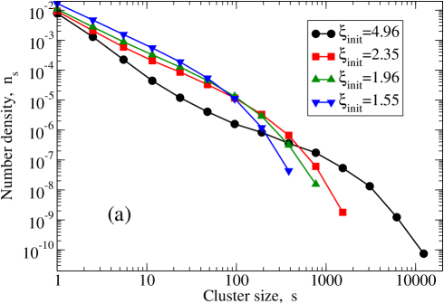
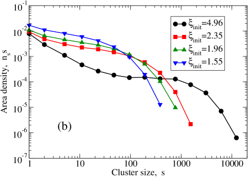
Figure 4: (a) Initial cluster size distributions, $n_{s}$ vs $s$, for the four simulations $\xi_{\rm init}$= (A) 4.96 (circles), (B) 2.35 (squares), (C) 1.96 (triangles up), and (D) 1.55 (triangles down). All are at coverage $\theta_{\rm init}=0.35$. (b) Corresponding data for the area density distributions, $n_{s}s$ vs $s$.Norms

Figure 3 shows typical snapshots for each of the four initial configurations at $\theta_{\rm init}=\theta_{\rm cutoff}$. For convenience, we label each class of initial configurations and each of the corresponding sets of desorption simulations as (A), (B), (C), and (D). Visual inspection of the snapshots immediately shows that configuration (A) is dominated by large clusters, while (B), (C), and (D) are dominated by progressively smaller clusters, respectively. This is confirmed by measurement of the mean cluster size $S$ for each of the configurations. Table 1 summarizes the parameters of the four initial configurations. The cluster number densities, $n_{s}$, of each of the four classes of initial configurations are shown in Fig. 4(a), and the corresponding area densities, $n_{s}s$, in Fig. 4(b). From Table 1, it is evident that reducing the mean cluster size results in reducing the correlation length as well. In our case, the four initial size distributions (A), (B), (C), and (D) show some similarity. The number density vs cluster size is always monotonically decreasing, showing a broad hierarchy of sizes. In configuration (A), the numbers of medium and small clusters are smaller, compared to the other configurations. The same can be said when we compare (B) to (C) and (C) to (D). However, the number density of larger clusters is smaller than the number density of smaller clusters in all of these four cases.

IV Simulation Results

IV.1 Coverage, Correlation Length, and Cluster Density

Our measurements are focused on the changes in morphology and dynamics due to the lateral diffusion as the initial configurations are varied. Table 2 summarizes the simulation results in terms of those changes for several coverages between $\theta_{\rm init}=0.35$ and $\theta=0.05$. The quantities measured are the increase of the correlation length, $\Delta\xi=\xi^{\prime}-\xi$, the fractional increase of the mean cluster size, $\delta S=(S^{\prime}-S)/S$, and the decrease in the desorption time required to reach a given coverage, $\Delta t(\theta)=t(\theta)-t^{\prime}(\theta)$ between the simulations without and with diffusion. The unprimed quantities in these expressions indicate the simulations without diffusion, while primes refer to the simulations with diffusion.

For $\theta=$ 0.32, 0.28, 0.25, 0.18, and 0.12, $\Delta\xi$ is always positive and increases as we decrease the initial correlation length from $\xi_{\rm init}$ = 4.96 to 2.35, 1.96, and 1.55, respectively. The coverage $\theta=0.05$ is close to the equilibrium value, in which the measurement results are small fluctuations around a constant value. At the earliest times (i.e., coverages closely below $\theta_{\rm init}$), the presence of diffusion retards the desorption process. This is indicated in Table 2 by the negative values of $\Delta t$ in simulations (B)-(C). Later in the simulations, the retardation is replaced by accelerated desorption, indicated by positive $\Delta t$.

In Fig. 5 we show the time evolution of the coverage $\theta$, with insets showing corresponding data for the correlation length $\xi$. The main parts of the figure confirm that diffusion induces a crossover from retarded desorption at early times, to accelerated desorption at late times. In part (A), corresponding to the large $\xi_{\rm init}=4.96$, the crossover to acceleration occurs almost immediately after the start of the desorption. [Thus deceleration is not seen for simulation (A) at the coverages included in Table 2.] Conversely, in part (D), corresponding to the small $\xi_{\rm init}=1.55$, the desorption remains retarded except at the very latest times. For the intermediate values of $\xi_{\rm init}$ shown in parts (B) and (C), the crossover can be clearly seen at an intermediate time. The insets, showing the effects of diffusion on the correlation length $\xi(t)$, display an analogous crossover from coarsening at early times to a reduction of $\xi$ at late times. We explain these competing effects of diffusion during the desorption process as follows.

Retardation. Due to their lack of lateral bonding, monomers are the most easily desorbed particles. However, lateral diffusion provides a mechanism for them to move into contact and bond with larger clusters or other monomers, thus reducing their subsequent rate of desorption. This process corresponds to a coarsening of the adsorbate configuration since it reduces the number of broken bonds [$\Sigma$ in Eq. (8)] by between two and six, without changing $\theta$.

Acceleration. Conversely, diffusion also provides a mechanism for a particle at the surface of a cluster to diffuse away and become a monomer. Following its detachment from the cluster, the new monomer has a higher desorption rate. While the initial detachment by diffusion clearly increases $\Sigma$, a following desorption of the resulting monomer will reduce $\Sigma$ by four and $\theta$ by $1/V$. The total change in $\xi$ may therefore be positive or negative, depending on the values of both these variables.

The balance between deceleration/coarsening and acceleration is determined by the fraction of the total coverage that consists of monomers and small clusters. This fraction is small for large $\xi_{\rm init}$. As a result, acceleration dominates as monomers “evaporate” from the large clusters. For small $\xi_{\rm init}$ the fraction of small clusters is large, leading to coarsening and deceleration of the desorption as excess monomers diffuse to join larger, more stable clusters. We discuss these effects in more detail below, in Sec. IV.2.

A complementary view of the effects of diffusion is provided by plotting the correlation length as a function of coverage, $\xi(\theta)$, as shown in Fig. 6. By hiding the effects of diffusion on the speed of desorption, this enables us to observe its influence on the adsorbate morphology as expressed by the correlation length at a specific coverage. Coarsening is seen at all coverages. The extent of the coarsening is very small for the largest $\xi_{\rm init}$, but increases gradually with decreasing $\xi_{\rm init}$. This is a reasonable result, since this view essentially represents a mapping of the adsorbate configuration onto a snapshot of one that could be produced due to Ostwald ripening by lateral monomer diffusion at fixed coverage (Kawasaki dynamics). Smaller $\xi_{\rm init}$ would then correspond to earlier times.

The effect of diffusion during the early stages of desorption is connected to the average distance between clusters. At a given coverage, this average distance is inversely proportional to the cluster density $\rho_{\delta}$. Figure 7 shows the results of cluster density measurements $\rho_{\delta}(\theta)$. Initially, the cluster density quickly drops by between 30% and 50% as $\theta$ decreases from its initial value. In simulation (A), it increases again after the initial drop, while in simulations (B), (C), and (D), it continues to decrease at a lower rate.

The effect of diffusion on the cluster density depends on the initial correlation length. In simulation (A), diffusion increases $\rho_{\delta}$ for all values of $\theta$ included in the figure. For the smaller values of $\xi_{\rm init}$ (B-D) there is a crossover from a reduction of $\rho_{\delta}$ for larger $\theta$ (early times) to an increase for smaller $\theta$ (later times). Comparing the coverages at which this crossover occurs with the plots of $\theta$ vs $t$ in Fig. 5, we see that they correspond approximately to the crossover times seen in that figure. Thus, a reduction of $\rho_{\delta}$ due to diffusion is correlated with retarded desorption, while an increase in $\rho_{\delta}$ is correlated with accelerated desorption.

IV.2 Cluster Size Distributions and Behavior of Individual Clusters

The morphological changes by diffusion are further illustrated by the area density histograms shown in Fig. 8. These figures show an example of the overall changes in $n_{s}s$ by diffusion at a particular coverage, $\theta=0.25$. Figure 8(A) shows a small change by diffusion, consistent with the very small increase of $\xi(\theta)$ by diffusion shown in Fig. 6(A). Figures 8(B-D) show more significant changes, consistent with larger changes in $\xi(\theta)$ by diffusion as we reduce $\xi_{\rm init}$. The changes amount to a depletion of intermediate-size clusters, which is partially compensated by transfer of coverage to larger clusters and monomers. This effect is observed for all coverages below $\theta_{\rm init}$.

Next we turn our attention to the dynamics of individual clusters. In Fig. 9 we show examples of the time evolution of the size $s$ of four individual, relatively large clusters picked from different simulations. The results were obtained with the cluster-tagging method discussed in Sec. II.3.2. We see a combination of shrinkage, occasional growth, splitting, and coalescence. Diffusion is seen to increase the frequencies of both coalescence and splitting events.

Figure 10 shows the average time evolution of the largest clusters at the beginning of the desorption stage (dark-colored clusters in Fig. 3), each picked out from realizations of the four classes of initial conditions (A–D), and each averaged over 100 independent runs. We immediately notice a qualitative similarity of these four average cluster behaviors to the general behavior of $\theta(t)$ in Fig. 5, including the crossover from retarded to accelerated desorption.

To further investigate the dynamics of the individual clusters, we pick out the 10 largest clusters from one realization of each of the four initial conditions (A-D) and measure the time to reach half their original volume (halftime $t_{\rm 1/2}$). Each result is averaged over 100 independent desorption runs. We then measure the acceleration,

$$\Delta t_{\rm 1/2}=t_{\rm 1/2}-t^{\prime}_{\rm 1/2}.$$ (12)

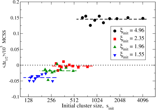
Figure 11: Halftime decrease with diffusion for the 10 largest clusters taken from a single realization of the initial conditions, $\xi_{\rm init}=$ (A) 4.96 (circles), (B) 2.35 (squares), (C) 1.96 (triangles up), and (D) 1.55 (triangles down). Each result is averaged over 100 independent desorption runs. Positive (negative) results correspond to acceleration (deceleration). The horizontal dashed lines represent the averages corresponding to each of the four data sets.

Figure 11 shows the decrease of the halftimes (positive for acceleration). We observe a crossover from acceleration to deceleration with decreasing $\xi_{\rm init}$. Comparing with the data for the total coverage $\theta$ vs $t$ in Fig. 5, we see that the behavior of the largest clusters in a single initial configuration is predictive of the overall acceleration/deceleration behavior of many initial configurations with the same $\xi_{\rm init}$ around the time when the average total coverage reaches half its initial value.

V Conclusions

Inspired by experimental results,HEY01 ; BAR95 ; BAR96 we studied the effects of lateral monomer diffusion on a lattice-gas model for the desorption of a submonolayer of adsorbate atoms from a single-crystal surface. Using large-scale kinetic Monte Carlo simulations, we found that diffusion produces two competing effects, and that the balance between the two depends on the shape of the cluster-size distribution at the onset of desorption.

Retardation of the desorption process is associated with the diffusion of monomers, which are weakly bound and thus easily desorbed, to achieve more strongly bound positions as members of multiatom clusters. This leads to a coarsening of the adsorbate configuration, expressed by an increase in the adsorbate correlation length $\xi$ and a depletion of the population of intermediate-size clusters. This effect is dominant when the adsorbate configuration is dominated by monomers and small clusters.

Acceleration of the desorption process is associated with the diffusion-induced “evaporation” of monomers from the perimeters of larger clusters to the surrounding two-dimensional, low-density “adsorbate gas,” where the absence of lateral bonding enhances their desorption rate. This effect is dominant when the adsorbate configuration is dominated by larger clusters. In contrast to the retardation, this mechanism can lead to an increase or a decrease in the correlation length, depending on the coverage and the number of broken bonds.

The crossover from retardation at early times to acceleration at later times occurs at a time that depends on the initial adsorbate configuration as shown in Fig. 5. This is a central result of our study. A complementary view is provided in Fig. 6, which shows the correlation length vs the total adsorbate coverage. Coarsening is observed at all coverages, but for a given coverage it is more pronounced when the initial configuration is dominated by monomers and small clusters. By “filtering out” the effects of diffusion on the overall desorption rate, this view emphasizes the Ostwald ripening driven by the coverage-conserving diffusion process. The corresponding transfer of coverage from intermediate-sized clusters to monomers and large clusters is illustrated in Fig. 8. The effect is strongest when the initial configuration is dominated by the smallest clusters.

Observation of the dynamics of individual clusters (Figs. 9 and 10) shows that individual clusters picked out for observation have similar dynamics as the overall system they belong to. The effect of diffusion on the dynamics of those clusters varies with the details of the initial configurations. In other words, the effect of diffusion on individual clusters depends on the size distributions, i.e., on the total environment surrounding each cluster.

We believe our observations can help interpret the details of experiments such as those reported in Refs. BAR95, , BAR96, , and HEY01, .

Table 1: Parameters for the four simulations. Mean cluster sizes $S$, correlation lengths $\xi$, and cluster densities $\rho_{\delta}$ are averages over 100 independent runs at coverage $\theta_{\rm init}=0.35$.

Init. Conf.	$\mu-\mu_{0}$ (Ads)	$S$	$\xi$	$\rho_{\delta}/10^{-3}$
A	0.40	2169.97	4.96	12.47
B	1.60	240.54	2.35	21.23
C	2.56	128.92	1.96	27.24
D	9.76	60.41	1.55	42.36

Table 2: Correlation length difference $\Delta\xi$, mean cluster size fraction $\delta S$, and time difference $\Delta t$. Primes signify simulations with diffusion.

Run	$\xi_{\rm init}$	$\theta$	$\Delta\xi=\xi^{\prime}-\xi$	$\delta S=(S^{\prime}-S)/S$	$~{}~{}~{}\Delta t=(t-t^{\prime})/10^{5}$
A	4.96	0.35	0.000	0.000	0.000
		0.32	0.069	0.011	0.016
		0.28	0.097	0.035	0.038
		0.25	0.083	0.055	0.066
		0.18	0.101	$-$0.054	0.146
		0.12	0.043	0.052	0.237
		0.05	0.004	$-$0.112	0.592
B	2.35	0.35	0.000	0.000	0.000
		0.32	0.190	0.235	$-$0.001
		0.28	0.216	0.194	0.000
		0.25	0.220	0.044	0.001
		0.18	0.194	0.075	0.009
		0.12	0.143	0.161	0.021
		0.05	$-$0.003	0.247	0.117
C	1.96	0.35	0.000	0.000	0.000
		0.32	0.275	0.268	$-$0.003
		0.28	0.304	0.202	$-$0.004
		0.25	0.300	0.173	$-$0.004
		0.18	0.253	0.134	$-$0.002
		0.12	0.167	0.108	0.003
		0.05	$-$0.000	0.072	0.069
D	1.55	0.35	0.000	0.000	0.000
		0.32	0.421	0.392	$-$0.005
		0.28	0.447	0.336	$-$0.008
		0.25	0.431	0.275	$-$0.012
		0.18	0.339	0.257	$-$0.017
		0.12	0.225	0.236	$-$0.018
		0.05	$-$0.009	0.099	0.030

$$\begin{array}[]{cc}{\rm(A)}&{\rm(B)}\\ {\includegraphics[scale={0.8}]{DROPLET1.eps}}&{\includegraphics[scale={0.8}]{DROPLET2.eps}}\\ {\rm(C)}&{\rm(D)}\\ {\includegraphics[scale={0.8}]{DROPLET3.eps}}&{\includegraphics[scale={0.8}]{DROPLET4.eps}}\\ \end{array}$$

Figure 3: Typical snapshots of the initial configurations of the four desorption simulations at $\theta_{\rm init}=0.35$, with $\xi_{\rm init}$ = (A) 4.96, (B) 2.35, (C) 1.96, and (D) 1.55, respectively. The largest cluster in each picture is colored dark.

$$\begin{array}[]{cc}{\includegraphics[scale={0.3}]{INSET1.eps}}&{\includegraphics[scale={0.3}]{INSET2.eps}}\\ {}\hfil&{}\hfil\\ {\includegraphics[scale={0.3}]{INSET3.eps}}&{\includegraphics[scale={0.3}]{INSET4.eps}}\\ \end{array}$$

Figure 5: The time evolution of $\theta(t)$ and $\xi(t)$ (insets) without and with diffusion, for simulations with $\xi_{\rm init}$ = (A) 4.96, (B) 2.35, (C) 1.96, and (D) 1.55, each averaged over 100 runs. Solid lines represent simulations without diffusion, and dashed lines represent simulations with diffusion.

$$\begin{array}[]{cc}{\includegraphics[scale={0.3}]{CorCov1.eps}}&{\includegraphics[scale={0.3}]{CorCov2.eps}}\\ {}\hfil&{}\hfil\\ {\includegraphics[scale={0.3}]{CorCov3.eps}}&{\includegraphics[scale={0.3}]{CorCov4.eps}}\\ \end{array}$$

Figure 6: The correlation length $\xi(\theta)$, without and with diffusion for the four simulations with $\xi_{\rm init}$= (A) 4.96, (B) 2.35, (C) 1.96, and (D) 1.55. Solid lines for simulations without diffusion, and dashed lines for simulations with diffusion. Note that $\theta$ decreases toward the right in this figure.

$$\begin{array}[]{cc}{\includegraphics[scale={0.3}]{DD1.eps}}&{\includegraphics[scale={0.3}]{DD2.eps}}\\ {}\hfil&{}\hfil\\ {\includegraphics[scale={0.3}]{DD3.eps}}&{\includegraphics[scale={0.3}]{DD4.eps}}\\ \end{array}$$

Figure 7: Cluster density $\rho_{\delta}(\theta)$ for the simulations with $\xi_{\rm init}$= (A) 4.96, (B) 2.35, (C) 1.96, and (D) 1.55. Open circles with solid lines represent simulations without diffusion, and full circles with dashed lines represent simulations with diffusion. Note that $\theta$ decreases toward the right in this figure.

$$\begin{array}[]{cc}{\includegraphics[scale={0.3}]{Nss1Y.eps}}&{\includegraphics[scale={0.3}]{Nss2Y.eps}}\\ \\ {\includegraphics[scale={0.3}]{Nss3Y.eps}}&{\includegraphics[scale={0.3}]{Nss4Y.eps}}\\ \end{array}$$

Figure 8: Area density distributions $n_{s}s$ vs $s$ at $\theta=0.25$ for simulations with $\xi_{\rm init}$= (A) 4.96, (B) 2.35, (C) 1.96, and (D) 1.55. Open circles with solid lines represent simulations without diffusion, and full circles with dashed lines represent simulations with diffusion.Norms

$$\begin{array}[]{cccc}{\rm(a)}&{\rm(b)}\\ {\includegraphics[scale={0.6}]{Shrink1.eps}}&{\includegraphics[scale={0.6}]{Shrink2.eps}}\\ {\rm(c)}&{\rm(d)}\\ {\includegraphics[scale={0.6}]{Shrink3.eps}}&{\includegraphics[scale={0.6}]{Shrink4.eps}}\\ \end{array}$$

Figure 9: The sizes of four clusters (a), (b), (c), and (d) as functions of time with and without diffusion. The solid line is for simulations without diffusion. In (a) we see a cluster shrinking. The diffusion accelerates the process for late times. In (b), (c), and (d) we see combinations of split, coalescence, growth, and shrinkage. In (b), a cluster splits, with diffusion accelerating the split. In (c), diffusion creates a series of brief coalescences and splits. In (d) diffusion creates a stable coalescence.

$$\begin{array}[]{cc}{\rm(A)}&{\rm(B)}\\ {\includegraphics[scale={0.6}]{TLargest1.eps}}&{\includegraphics[scale={0.6}]{TLargest2.eps}}\\ {\rm(C)}&{\rm(D)}\\ {\includegraphics[scale={0.6}]{TLargest3.eps}}&{\includegraphics[scale={0.6}]{TLargest4.eps}}\\ \end{array}$$

Figure 10: Time evolution of the largest cluster, each picked out from the simulations with $\xi_{\rm init}$= (A) 4.96, (B) 2.35, (C) 1.96, and (D) 1.55, and each averaged over 100 runs. Solid lines represent simulations without diffusion, and dashed lines represent simulations with diffusion.