Abstract

Polarizers are key components in optical science and technology. Thus, understanding the action of a polarizer beyond oversimplifying approximations is crucial. In this work, we study the interaction of a polarizing interface with an obliquely incident wave experimentally. To this end, a set of Mueller matrices is acquired employing a novel procedure robust against experimental imperfections. We connect our observation to a geometric model, useful to predict the effect of polarizers on complex light fields.

OCIS codes: (120.5410) Polarimetry; (260.2130) Ellipsometry and polarimetry; (260.5430) Polarization.

1 Introduction

Electromagnetic radiation is described as a vector field and, thus, the orientation of the electric field vector, known as polarization, is of great importance, both in classical and quantum optics. Polarized states of the light field are often prepared and measured using polarizers and analyzers, respectively, which can refer to the same device. The physical implementation of such polarizing elements can be very different according to the application the device is designed for. For example, the liquid crystal display (LCD) industry has refined their polarizer design over the past decades to achieve the outstanding performance that these devices show today [1, 2, 3].

From a more fundamental point of view, it is desirable to work with a generic polarizer model, which is computationally convenient and takes into account the geometric nature of the problem while being suitable to describe a wide range of polarizers. Such geometric models are currently used in the theoretical literature [4, 5]. However, to the knowledge of the authors, they lack experimental validation, in particular for unusual corner cases. Even for wide-view LCDs, the propagation angle inside the polarizing element is not as steep as in our measurements. Since any device which qualifies as a polarizer acts similarly on a normally incident light beam, these obliquely incident waves can be used to establish a realistic geometric model and demonstrate its validity.

In this article, the Mueller matrix of a commercial polarizer made of elongated nano-particles shall be measured. Reconstructing such a matrix from potentially noisy experimental data is challenging and prone to errors [6]. We solve this problem using a self-calibrating polarimeter, which additionally warrants that the result is physically acceptable [7, 8]. Our method combines a number of ideas discussed in the literature [9, 10, 11, 12].

This article is structured as follows: First, we introduce and illustrate polarization and polarizer models. Then, we propose a Mueller matrix polarimeter, which is robust against experimental imperfections and does not rely on precision optics nor calibrated reference samples. Finally, we employ this setup to obtain Mueller matrices for a commercial polarizer and connect the observation to its microscopic structure. Motivated by recent theoretical and experimental work connecting the action of a tilted polarizer to a beam shift phenomenon [13, 14], we extend our studies to include the unusual case of almost grazing incidence.

2 Polarization of a light beam

In this work, we use both, Jones and Mueller-Stokes calculi, to represent the polarization properties of the light field. There are two key differences between both approaches. First, the former method works with the electric field, while the latter depends only on intensities, which can be directly measured. And second, the Mueller-Stokes representation is more general since it allows for describing unpolarized states of light and depolarizing optical elements.

For our purpose, a collimated, polarized light beam can be approximated as a planar wave field. A plane wave is completely determined by the complex envelope $\bm{J}=E_{x}\bm{\hat{x}}+E_{y}\bm{\hat{y}}$ of its electric field $\bm{E}(\bm{r},t)=\operatorname{Re}\left[\bm{J}\,\exp(i(\bm{k}\cdot\bm{r}-\omega t))\right]$, where $\bm{k}=k\bm{\hat{z}}$ is the wave vector. The complex column-vector $\bm{J}$ has become known as the Jones vector [15, 16].

Alternatively, the state of polarization of any light beam can be described by a set of four real Stokes parameters [17]

$$\begin{pmatrix}S_{0}\\ S_{1}\\ S_{2}\\ S_{3}\end{pmatrix}=\begin{pmatrix}I_{0\mathrm{\SIUnitSymbolDegree}}+I_{90\mathrm{\SIUnitSymbolDegree}}\\ I_{0\mathrm{\SIUnitSymbolDegree}}-I_{90\mathrm{\SIUnitSymbolDegree}}\\ I_{+45\mathrm{\SIUnitSymbolDegree}}-I_{-45\mathrm{\SIUnitSymbolDegree}}\\ I_{R}-I_{L}\end{pmatrix}=\begin{pmatrix}|E_{x}|^{2}+|E_{y}|^{2}\\ |E_{x}|^{2}-|E_{y}|^{2}\\ E_{x}E_{y}^{\ast}+E_{x}^{\ast}E_{y}\\ i(E_{x}E_{y}^{\ast}-E_{x}^{\ast}E_{y})\end{pmatrix}\text{,}$$ (1)

where $I_{\alpha}$ is the intensity of the light beam transmitted across a linear polarizer oriented at an angle $\alpha$ with respect to the $\bm{\hat{x}}$ axis and $I_{R,L}$ is the right- or left-handed circularly polarized component of the intensity.

The four Stokes parameters $S_{\mu}$ are related to the Jones vector $\bm{J}$ through the dyadic product of the Jones vector and its conjugate transpose $\bm{J}^{\dagger}$ multiplied with the Pauli matrix $\sigma^{(\mu)}$ corresponding to each Stokes parameter [18]:

$$\bm{S}_{\mu}=\operatorname{Tr}\left[\left(\bm{J}\otimes\bm{J}^{\dagger}\right)\sigma^{(\mu)}\right]\text{.}$$ (2)

The trace operation is in general irreversible. Obviously, every Jones vector $\bm{J}=(E_{x},E_{y})^{\text{T}}$ can be converted into a set of Stokes parameters, whereas the reverse is not true. In this article, we choose a basis

$$\sigma^{(0)}=\frac{1}{\sqrt{2}}\begin{pmatrix}1&0\\ 0&1\end{pmatrix},\sigma^{(1)}=\frac{1}{\sqrt{2}}\begin{pmatrix}1&0\\ 0&-1\end{pmatrix},\sigma^{(2)}=\frac{1}{\sqrt{2}}\begin{pmatrix}0&1\\ 1&0\end{pmatrix},\sigma^{(3)}=\frac{1}{\sqrt{2}}\begin{pmatrix}0&-i\\ i&0\end{pmatrix},$$

consistent with the definition of the Stokes parameters used in popular textbooks [17].

Both approaches allow for a matrix calculus to describe linear operations affecting the state of polarization [16],

$$\bm{J}^{\text{in}}\rightarrow\bm{J}^{\text{out}} =T\,\bm{J}^{\text{in}}\text{,}$$ (3)

$$\bm{S}^{\text{in}}\rightarrow\bm{S}^{\text{out}} =M\,\bm{S}^{\text{in}}\text{,}$$ (4)

where $T$ and $M$ are called Jones and Mueller matrices, respectively.

3 Geometric Polarizer Models

Generally, a polarizer is understood to project the light field onto a particular state of polarization. For a plane wave impinging perpendicularly onto a linear polarizer, this state is trivially given by the orientation of the polarizing axis. In any other case, we need to work with a suitable model taking into account the physical nature of the interaction. For polarizers, for which the polarizing effect takes place at an interface between two media, e.g. reflection at the Brewster angle, this problem is solved by applying the well-known boundary conditions or Fresnel formulas.

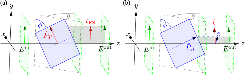
Fig. 1: Geometric interpretation of polarizer models. A plane wave with its electric field $\bm{E}^{\text{in}}$ in the $\bm{\hat{x}}\bm{\hat{y}}$-plane interacts with a tilted polarizer not parallel to this plane. Our goal is to connect the orientation $\theta$, $\phi$ of the polarizer to the direction of the transmitted field component $\bm{E}^{\text{out}}$. (a) Fainman and Shamir [4] suggested to find this direction $\bm{t}_{\text{FS}}$ by projecting a vector $\bm{\hat{P}}_{T}$ interpreted as the polarizer’s transmitting axis onto the $\bm{\hat{x}}\bm{\hat{y}}$-plane. (b) The polarizer in question is made of elongated particles, all with their long axes oriented in direction of $\bm{\hat{P}}_{A}$. Thus, our absorbing model makes of use of the projection $\bm{a}$ of the absorbing axis $\bm{\hat{P}}_{A}$. The field component parallel to $\bm{a}$ is scattered and eventually absorbed. Consequently, the transmitted field is polarized in direction of $\bm{\hat{t}}$, orthogonal to $\bm{a}$.

Fainman and Shamir (FS) have constructed a convenient geometrical model applicable to polarizers that do not change the direction $\bm{\hat{z}}$ of wave propagation [4]. They allow for an arbitrary orientation of the polarizer and assert that it can be completely described with a three-dimensional unit vector $\bm{\hat{P}}_{T}$. FS make use of the transversality of the electric field vector and conclude that the effect of a polarizer reduces to the projection onto an effective transmitting axis $\bm{\hat{t}}_{\text{FS}}$ (illustrated in Fig. 1(a)). In their model, the unit vector $\bm{\hat{t}}_{\text{FS}}\propto\bm{\hat{P}}_{T}-(\bm{\hat{z}}\cdot\bm{\hat{P}}_{T})\bm{\hat{z}}$ is found by projecting the polarizer’s transmitting axis $\bm{\hat{P}}_{T}$ onto the plane of the electric field perpendicular to the direction of wave propagation $\bm{\hat{z}}$.

Fainman and Shamir’s approach is practically useful since establishing an effective transmitting axis reduces the complexity of the intrinsically three-dimensional problem to an operation on the two-dimensional Jones vector $\bm{J}$. For any orientation of the polarizer, the resulting Jones matrix $T_{\text{FS}}=\bm{\hat{t}}_{\text{FS}}\bm{\hat{t}}_{\text{FS}}^{\text{T}}$ is a projector as expected for an ideal polarizer. However, their recipe does not take into account the physical nature of the interaction.

In this work, we attempt to adapt FS’s approach to our observation. In particular, we study a polarizing element made of anisotropic absorbing and scattering particles. The ensemble of these elementary absorbers shall be oriented with their absorbing axes $\bm{\hat{P}}_{A}$ parallel to each other. Analogously to the transmitting case, we interpret the projection of this unit vector $\bm{\hat{P}}_{A}$ as an effective absorbing axis

$$\bm{\hat{a}}=\frac{\bm{\hat{P}}_{A}-(\bm{\hat{P}}_{A}\cdot\bm{\hat{z}})\bm{\hat{z}}}{\sqrt{1-(\bm{\hat{P}}_{A}\cdot\bm{\hat{z}})^{2}}}\text{.}$$ (5)

If this interpretation holds true, the light field after transmission across an absorbing polarizer becomes

$$\bm{E}^{\text{in}}\rightarrow\bm{E}^{\text{out}}=\bm{E}^{\text{in}}-(\bm{E}^{\text{in}}\cdot\bm{\hat{a}})\bm{\hat{a}}\text{.}$$ (6)

As above, the corresponding Jones matrix $T_{A}=1-\bm{\hat{a}}\bm{\hat{a}}^{\text{T}}=\bm{\hat{t}}\bm{\hat{t}}^{\text{T}}$ is a projector, where $\bm{\hat{t}}=\bm{\hat{z}}\times\bm{\hat{a}}$ can be interpreted as the effective transmitting axis as illustrated in Fig. 1(b). While Eq. (5) is structurally equivalent to Fainman and Shamir’s construction, our model coincides with their approach only for normal incidence. Generally, our absorbing model $T_{A}=1-\bm{\hat{a}}\bm{\hat{a}}^{\text{T}}$ differs from the FS case $T_{\text{FS}}=\bm{\hat{t}}_{\text{FS}}\bm{\hat{t}}_{\text{FS}}^{\text{T}}$. We want to note that the absorbing model can be found alternatively by treating the sub-wavelength structure of the polarizer as a composite material, which behaves as an anisotropic absorbing crystal [19].

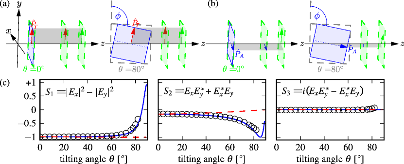
Fig. 2: State of polarization transmitted across a polarizer rotated around the vertical axis $\bm{\hat{y}}$ by an angle $\theta$, keeping the angle $\phi=94.5\mathrm{\SIUnitSymbolDegree}$ between the absorbing axis and $\bm{\hat{y}}$ constant. (a) Visualization of the FS model [4]: The projection of the polarizer’s transmitting axis $\bm{\hat{P}}_{T}$ (red arrow) onto the plane of the electric field (green plane) determines the transmitted field component (green arrow). (b) Visualization of the absorbing polarizer model (6): The projection of the polarizer’s absorbing axis $\bm{\hat{P}}_{A}$ (blue arrow) onto the plane of the electric field (green plane) determines the absorbed field component. (c) Experimental data points (black circles) compared to both models. The dashed red line depicts the original FS model, while the solid blue line describes the analogously constructed absorbing model. The data shows the polarizance vector $M_{i0}$ [20] acquired as a part of our Mueller matrix measurement. This is the state of polarization after transmission across the polarizer if the incident wave is unpolarized. Only the absorbing model explains the drastic change of the transmitted state of polarization observed when the polarizer is tilted.

We rely on empirical evidence to decide, whether any of those two geometric models adequately describes our real-world polarizer. To this end, we compare the state of polarization transmitted across the polarizer to the one predicted by both models [Fig. 2]. This shows that our polarizer can be approximated as a projector. When tilted, the state of polarization, the device projects onto, is given by Eq. (6).

This simple absorbing model, Eq. (6), is the first main result of this article. Using the Mueller matrix measurements reported in the following sections, we can establish a phenomenological model and connect the observation to a physical picture of the light field’s interaction with the nano-particles.

4 Mueller Matrix measurement

In this section, we present a method to measure the Mueller matrix of an arbitrary optical element, which is robust against experimental imperfections, such as noise and systematic errors. With this least squares based estimation, we can gain full information about the polarization properties of the device-under-test performing only a limited number of intensity measurements. The method employs a polarizer, a polarization beam splitter as an analyzer, and two rotating wave plates to select the states of polarization [Fig. 3(a)].

In any of these measurements, the observed intensities

$$I_{ij}=\frac{1}{2}\,(\bm{S}_{j}^{\text{out}})^{\text{T}}\,M\,\bm{S}_{i}^{\text{in}}$$ (7)

depend on the first waveplate, which prepares a state of polarization $\bm{S}_{i}^{\text{in}}$, the unknown Mueller matrix $M$ describing the device-under-test, and the state of polarization $\bm{S}_{j}^{\text{out}}$, we project onto at the detection stage. Here, the row vector $\frac{1}{2}\bm{S}^{T}$ describes the action of an analyzer transmitting the state of polarization given by $\bm{S}$. Applied to any Stokes vector, this yields the transmitted intensity.

In principle, a generic real-valued $4\times 4$ matrix $M$ is unambiguously determined by 16 equations like Eq. (7). However, the measured intensities $I_{ij}^{\text{E}}$, where the superscript $E$ denotes experimental values, can be noisy. Thus, acquiring more than 16 values helps to reduce both statistical and systematic errors significantly. To this end, instead of solving a linear system of equations, we pick the Mueller matrix $M^{\text{LS}}$ from the set of all possible Mueller matrices, such that

$$\varepsilon(M^{\text{LS}})=\sum_{i,j}\left|\frac{1}{2}\,(\bm{S}_{j}^{\text{out}})^{\text{T}}\,M^{\text{LS}}\,\bm{S}_{i}^{\text{in}}-I_{ij}^{\text{E}}\right|^{2}$$ (8)

becomes minimal.

A Mueller matrix $M$ is physically acceptable [6, 7, 8] if and only if its matrix elements

$$M_{ab}=\operatorname{Tr}\left[H\left(\sigma^{(a)}\otimes{\sigma^{(b)}}^{\ast}\right)\right]$$ (9)

are a function of a Hermitian matrix $H$ with non-negative eigenvalues [6]. Any such matrix $H=H^{\dagger}$ can be expressed using a set of 16 real numbers $\{h_{1},\dots,h_{16}\}$. Therefore, these 16 parameters span the vector space of physical Mueller matrices and the set $\{h_{1}^{\text{LS}},\dots,h_{16}^{\text{LS}}\}$ which minimizes Eq. (8) yields to the best estimate $M^{\text{LS}}$ for the actual Mueller matrix.

If the states of polarization $\bm{S}$ are not known precisely, we can find these parameter employing a procedure similar to the one described above. Interestingly, this requires no a priori information beyond the knowledge that the polarization states $\bm{S}$ are prepared using polarizers and birefringent retarders. To this end, the device-under-test is removed from the beam path. Using the same procedure as for the actual measurement, a set of intensities $I_{ij}^{\text{cal}}$ is acquired, which characterizes the setup.

Theoretically, this calibration run corresponds to substituting $M^{\text{LS}}$ in Eq. (8) with the identity matrix (Mueller matrix of empty space). Additionally, we express the abstract Stokes vectors $(\bm{S}_{j}^{\text{out}})^{\text{T}}=(\bm{S}_{H,V})^{T}\,M^{\text{out}}_{j}$ and $\bm{S}_{i}^{\text{in}}=M^{\text{in}}_{i}\,\bm{S}_{H}$ in terms of Mueller matrices $M^{\text{out}}_{j}$ and $M^{\text{in}}_{i}$, which physically describe our measurement device. The Stokes vectors $\bm{S}_{H,V}$ represent horizontally or vertically polarized states, respectively. In our experiment, those are the states transmitted or reflected by a polarizing beam splitter [Fig. 3(a)]. This yields:

$$\varepsilon(M^{\text{LS}})=\sum_{i,j}\left|\frac{1}{2}(\bm{S}_{H,V})^{T}\,M_{j}^{\text{out}}\,M_{i}^{\text{in}}\,\bm{S}_{H}-I_{ij}^{\text{cal}}\right|^{2}\text{.}$$ (10)

In particular, $M^{\text{in}}_{i}(\alpha_{i}^{\text{in}},\rho^{\text{in}})$ represents the first wave plate with the retardation $\rho^{\text{in}}$ and its fast axis oriented at an angle $\alpha_{i}^{\text{in}}$ with respect to the $\bm{\hat{x}}$ axis. Analogously, $M^{\text{out}}_{j}(\alpha_{j}^{\text{out}},\rho^{\text{out}})$ describes the second wave plate.

Since we cannot fully rely on the manufacturer to specify retardation and orientation of the fast axis with the desired accuracy, those values are treated as unknown. Nevertheless, employing motorized rotation stages, we can precisely reproduce relative movements $\Delta\alpha_{i}=\alpha_{i+1}-\alpha_{i}$ of both wave plates, where, for example, $\Delta\alpha_{i}=\Delta\alpha=22.5\mathrm{\SIUnitSymbolDegree}$. Thus, our measurement setup is completely described by four parameters, $\alpha_{0}^{\text{in}}$, $\rho^{\text{in}}$, $\alpha_{0}^{\text{out}}$, and $\rho^{\text{out}}$, which are to be found with this calibration procedure. The set of parameters which minimizes Eq. (10) yields the states of polarization $\bm{S}_{i}^{\text{in}}$ and $\bm{S}_{j}^{\text{out}}$ relevant for our experiment.

As soon as these calibration parameters are known, Eq. (8) only depends on properties of the device-under-test. Minimizing Eq. (8) yields to the best experimental estimate for the actual Mueller Matrix $M^{\text{LS}}$ describing the device.

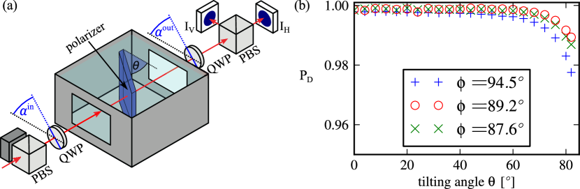
Fig. 3: (a) Scheme of the Mueller matrix measurement. Using a collimated light beam (wavelength $\lambda=795\,\mathrm{n}\mathrm{m}$), polarizing beam splitters (PBS), quarter wave plates (QWP), and two photo detectors I${}_{\text{H}}$ and I${}_{\text{V}}$, the effect of an unknown sample on the polarization can be measured. For both QWPs, we use 6 different settings $\alpha^{\text{in/out}}$ of their fast axes. Our sample is a commercial glass polarizer submerged in an index-matching liquid, which can be rotated around the vertical axis such that the incident beam impinges under an angle $\theta$. This setup allows to study the polarizing effect of the metal nano-particles, the polarizer is made of, without interference from the glass surfaces. (b) Observed depolarization index $P_{D}$ [21] as a function of the orientation $\phi$, $\theta$ of the polarizer relative to the incident beam. $P_{D}=1$ describes a non-depolarization sample while $P_{D}=0$ indicates a total depolarizer.

5 Experiment

In our experiment, we study a polarizing interface, made of anisotropically absorbing nano-particles. To this end, we employ a commercial “Corning Polarcor” polarizer, made of a glass substrates with 25 to 50 µ m  thick polarizing layers on each face. These layers contain embedded, elongated and oriented silver particles.

We are particularly interested in the interaction beyond the trivial case of normal incidence. However, at larger angles of incidence $\theta$, the existence of surfaces becomes problematic since a light beam propagating across an interface experiences both, a change of its direction of propagation (Snell’s law) and of its polarization (a consequence of Fresnel’s formulas) [17]. These well-known effects are unrelated to the action of the actual polarizing layer inside the glass substrate. Thus, we avoid such surface effects by submerging the polarizer in a tank filled with an index matching liquid (Cargille laser liquid 5610). The refractive index of this liquid ($n_{L}=1.521$) matches with the one of the polarizer’s substrate ($n_{G}=1.517$).

Each measurement run consists of $6\times 6$ steps, acquiring two intensity values per step. Every step uses a different combination of the two wave plates’ angles. For the required calibration run, we remove the polarizer from the beam path, but keep the container with the index-matching liquid. Neither the liquid nor the glass windows were observed to affect the state of polarization. From this calibration data, we learn that both of our quarter-wave plates perform within their specifications ($\alpha_{0}^{\text{in}}=2.57\mathrm{\SIUnitSymbolDegree}$, $\rho^{\text{in}}=\pi/2+0.008\,\mathrm{rad}$, $\alpha_{0}^{\text{out}}=0.89\mathrm{\SIUnitSymbolDegree}$, and $\rho^{\text{out}}=\pi/2+0.019\,\mathrm{rad}$). Nevertheless, knowledge of these parameters is crucial to perform a highly accurate Mueller matrix reconstruction.

Our goal is three-fold: First, we attempt to establish a phenomenological model taking into account the finite extinction ratio exhibited by real-world polarizers. Then, we demonstrate that this model accurately predicts the behaviour for a wide range of parameters. And finally, we connect the observation to the interaction of the light field with the ensemble of nano-particles.

To this end, we perform three series of measurement runs for different orientations $\phi$ of the polarizer’s absorbing axis, each for a large number of tilting angles $0\mathrm{\SIUnitSymbolDegree}\leq\theta\leq 82\mathrm{\SIUnitSymbolDegree}$. We apply the least-squares method described above to find the Mueller matrices describing our polarizer.

Results acquired with this method can be reproduced precisely. Comparing independent measurements for the same configuration shows that the statistical error of any Mueller matrix element $M_{ab}$ is less then $10^{-3}$. Furthermore, our data indicates that the results are also accurate. The sample, we have studied is a linear polarizer. For normal incidence ($\theta=0\mathrm{\SIUnitSymbolDegree}$), the transmittance across such a polarizer does not depend on the helicity of the incident beam and the transmitted beam is linearly polarized. The corresponding Mueller matrix elements $|M_{03}|<0.01$ and $|M_{30}|<0.01$ clearly vanish for all relevant measurements. Thus, we estimate systematic errors to be below $10^{-2}$.

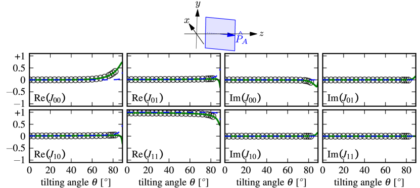
Fig. 4: Jones matrix representation of the operation a light beam experiences when passing across our polarizer. The polarizer’s absorbing axis $\bm{\hat{P}}_{A}$ is oriented almost horizontally ($\phi=89.2\mathrm{\SIUnitSymbolDegree}$) and rotated around the vertical axis $\bm{\hat{y}}$ by an angle $\theta$. The experimental data points (black circles) are calculated from our measured Mueller matrices. Ignoring an irrelevant global phase, we set $\operatorname{Im}(J_{11})=0$. Our phenomenological model, described by $T_{P}$, is depicted using solid green lines. Dashed blue lines show the geometric absorbing model given by $T_{A}$.

All measured Mueller matrices are practically non-depolarizing [Fig. 3(b)]. This means that a Jones matrix representation suffices to describe our sample. The data series with the absorbing axis oriented almost horizontally [Fig. 4] shows clearly that both the transmittance and the extinction ratios decreases with the tilting angle $\theta$. This behaviour cannot be described by a perfect projector as in the geometric models discussed earlier. Thus, we propose to generalize the projection rule, Eq. (6), to include two transmission coefficients $\tau_{a}$ and $\tau_{t}$ for states of polarization parallel and perpendicular to the effective absorbing axis:

$$\bm{E}^{\text{in}}\rightarrow\bm{E}^{\text{out}}=T_{P}\,\bm{E}^{\text{in}}\quad\text{ with }T_{P}=\tau_{a}\,\bm{\hat{a}}\bm{\hat{a}}^{\text{T}}+\tau_{t}\,\bm{\hat{t}}\bm{\hat{t}}^{\text{T}}\text{.}$$ (11)

Fig. 5: Reduced Mueller matrices $M^{\prime}=\frac{1}{M_{00}}\,M$ describing the tilted polarizer for two different orientations of its absorbing axis $\phi$. Our polarizer model (solid lines) agrees well with the experimental data (markers). The model, we have employed, is deterministic. The small deviation from the model occurs for large tilting angles $\theta$, where the devices is slightly depolarizing (compare Fig. 3(b)). Depolarization effects cannot be modelled using Jones calculus as employed by our model.

Using an ansatz implied by the qualitative behaviour of the data set shown in Fig. 4, we apply a curve-fitting algorithm to this data set, which yields:

$$\tau_{t}(\theta) =\exp(-0.025/\cos(\theta))\quad\text{ and}$$ (12a)

$$\tau_{a}(\theta) =0.89\,\exp(-6.70\,\cos(\theta))-i\,0.62\,\exp(-13.6\,\cos(\theta))\text{.}$$ (12b)

Equations (11) and (12) constitute a phenomenological model for our polarizer suitable to predict Jones and Mueller matrices for any choice of the parameters $\theta$ and $\phi$. In Fig. 5, we demonstrate that this model accurately agrees with our observation for different configurations.

Equation Eq. (12a) is a variant of Beer’s law [17, 22] and describes how the absorption scales with the increasing effective thickness of the sample when tilted. The modulus square $|\tau_{a}|^{2}>0$ of Eq. (12b) accounts for the transmittance for crossed polarization, i.e. the fact that even if the electric field is polarized parallel to the effective absorbing axis, the absorption is not 100%. The phase of the complex parameter $\tau_{a}$ indicates that this field component is scattered with a phase determined by the orientation of the nano-particles relative to the incoming wave.

For small tilting angles $\theta<45\mathrm{\SIUnitSymbolDegree}$, the observation agrees with the prediction of the geometric absorbing model $T_{A}$. Close to grazing incidence $\theta\rightarrow 90\mathrm{\SIUnitSymbolDegree}$, the latter deviates, which we can understand in a physical picture. The particles embedded in our polarizer are cigar-shaped [23, 24]. Relevant for the polarization effect is the coupling of the light field to their long axes $\bm{\hat{P}}_{A}$. By design, the wavelength is close to the resonance of the particles’ long axes. At normal incidence, the scattering and absorption is strong for states of polarization parallel to the long axis and negligible in the orthogonal case.

When the polarizer is tilted, only the component of the electric field vector directed along the particles’ absorbing axis $\bm{\hat{P}}_{A}$ takes part in the interaction. Thus, the effect of a single particle decreases proportionally to $\cos(\theta)$ as the coupling becomes less efficient.

The thickness of the polarizing layer guarantees that a light beam interacts with multiple particles while propagating across the device. Consequently, the observed extinction ratio is significantly larger than expected for a single particle. Our phenomenological model subsumes the sophisticated effect of this ensemble using only two functions $\tau_{a}(\theta)$ and $\tau_{t}(\theta)$, which can be directly measured.

6 Conclusion

We have presented a Mueller matrix polarimeter making use of inexpensive linear polarizers and arbitrary retarding elements. Our least squares optimization approach is fast, yet accurate and precise. In particular, we have used this setup to study the effect a tilted polarizer has on the light field.

Incidentally, linear polarizers are also popular as reference samples to characterize such measurement devices. Our data indicates that the combined statistical and systematic error of any matrix element is less than $0.01$, while for polarimeters of comparable speed and feasibility, deviations between $0.03$ and $0.10$ per matrix element are typical [25]. In fact, our method is comparable with the accuracy achieved by more sophisticated calibration techniques requiring the use of multiple reference samples [26].

Finally, we have shown that a real-world polarizer, even when tilted, can be modeled geometrically. Using only the projection of the absorbing axis yielded already to an acceptable approximation for the collective action of the nano-particle ensemble. It was demonstrated that the finite extinction ratio of realistic polarizers can be taken into account phenomenologically, including configurations close to grazing incidence. We are confident that future work will connect the observation to a detailed microscopic study of such nano-particles and their interaction with the light field.