Dyson-Schwinger study of chiral density waves in QCD

Abstract

The formation of inhomogeneous chiral condensates in QCD matter at nonzero density and temperature is investigated for the first time with Dyson-Schwinger equations. We consider two massless quark flavors in a so-called chiral density wave, where scalar and pseudoscalar quark condensates vary sinusoidally along one spatial dimension. We find that the inhomogeneous region covers the major part of the spinodal region of the first-order phase transition which is present when the analysis is restricted to homogeneous phases. The triple point where the inhomogeneous phase meets the homogeneous phases with broken and restored chiral symmetry, respectively, coincides, within numerical accuracy, with the critical point of the homogeneous calculation. At zero temperature, the inhomogeneous phase seems to extend to arbitrarily high chemical potentials, as long as pairing effects are not taken into account.

The properties of strong-interaction matter under extreme conditions, such as high temperature or density, and the corresponding phase structure of Quantum Chromodynamics (QCD) are subject of extensive theoretical and experimental investigations [1, 2]. At vanishing net baryon density, first-principle lattice gauge calculations have revealed that the approximate chiral symmetry of QCD, which is spontaneously broken at low temperature, gets restored at high temperature in a cross-over transition [3, 4]. At low temperature and high baryon density, where lattice calculations are inhibited by the sign problem, effective model studies typically predict that chiral symmetry is restored in a first-order phase transition, which weakens with increasing temperature and eventually ends at a critical point [5]. More recently, this picture was confirmed with Dyson-Schwinger equations (DSEs) applied to QCD [6, 7, 8, 9].

A basic assumption in these investigations was that the phases are homogeneous, i.e., in particular, the chiral order parameter is constant in space. On the other hand, phases with non-uniform chiral order parameters have been proposed already long time ago, see Ref. [10] for a brief historical review. Starting with Migdal’s $p$-wave pion condensation [11], the idea was generalized to relativistic systems [12, 13, 14] and studied in high-density QCD with large number of colors, applying weak-coupling methods [15, 16]. More recently, it gained new attention after it was found in effective models that the first-order chiral phase boundary between homogeneous phases is covered completely by an inhomogeneous phase [17, 18].

The aim of our work is to study the chiral phase transition with the possibility of inhomogeneous condensates in strong-coupling QCD with DSEs. We restrict ourselves to a so-called chiral density wave (CDW), where the chiral condensate rotates along the chiral circle, when moving into a fixed direction. Specifically, the scalar and pseudoscalar condensates behave like

$$\langle\bar{q}q\rangle\propto\cos(Qz)\,,\quad\langle\bar{q}i\gamma_{5}\tau_{3}q\rangle\propto\sin(Qz)\,,$$ (1)

with $Q$ being the modulus of a wave vector, which we have chosen to point into the $z$ direction. Moreover, as indicated by the Pauli matrix $\tau_{3}$, we have chosen the third isospin component of the pseudoscalar condensate. Assuming isospin invariance of the QCD Lagrangian, this can be done without loss of generality.

Figure 1: Dyson-Schwinger equation for the full quark propagator. Plain lines represent quark propagators, the curly line the gluon propagator. Thick dots represent dressed quantities.

The DSE for the dressed quark propagator $S$ is diagrammatically depicted in Fig. 1. In coordinate space with Euclidean metric, it is given by $S^{-1}(x,x^{\prime})=Z_{2}\left(S_{0}^{-1}(x,x^{\prime})+\Sigma(x,x^{\prime})\right)$, depending on two space-time variables, $x$ and $x^{\prime}$. $S_{0}$ denotes the bare propagator, $\Sigma$ the selfenergy and $Z_{2}$ is the wave-function renormalization constant of the quark field.

In homogeneous, i.e., translationally invariant matter, the propagator depends only on the relative coordinate $x-x^{\prime}$. In momentum space, this translates into a dependence on a single 4-momentum, and the inverse propagator at temperature $T$ and chemical potential $\mu$ can be parametrized as

$$S_{\mathit{hom}}^{-1}(p)=-i\omega_{n}\gamma_{4}C(p)-i{\vec{\gamma}}\cdot{\vec{p}}A(p)+B(p)\,,$$ (2)

with $p:=(\vec{p},p_{4}=\omega_{n}+i\mu)$, the Matsubara frequencies $\omega_{n}=(2n+1)\pi T$, and three dressing functions $A$, $B$, and $C$. In vacuum, due to Lorentz covariance, these functions depend on $p^{2}$ only and $A(p)=C(p)$. The wave-function renormalization constant $Z_{2}$ is then fixed by the condition that $A(p)|_{p^{2}=\nu^{2}}=1$ at an arbitrary renormalization point $\nu$. This prescription remains valid for our analysis of inhomogeneous phases since $Z_{2}$ is always fixed in vacuum, which is homogeneous.

In inhomogeneous matter, the quark selfenergy and, hence, the propagator depend separately on both coordinates $x$ and $x^{\prime}$, or, equivalently, on the relative coordinate $x-x^{\prime}$ and the center of momentum coordinate $(x+x^{\prime})/2$. In momentum space they thus depend on two momenta, and the DSE reads

$$S^{-1}(p,p^{\prime})=Z_{2}\left(S_{0}^{-1}(p,p^{\prime})+\Sigma(p,p^{\prime})\right).$$ (3)

Here $p$ and $p^{\prime}$ correspond to the out- and ingoing momenta of the quark, which do not need to be identical. Physically, this means that the inhomogeneous condensates carry momentum, so that the quark can change its momentum by scattering off the condensate.

The (inverse) propagator can be viewed as a continuous matrix in momentum space. For the formal manipulations to be discussed below it is useful to introduce a finite quantization volume $V$ in 3-space and take periodic boundary conditions. Thus, together with the finite extent in the imaginary time direction, the 4-volume is finite as well, ${\cal V}=V\times[0,1/T]$, and the 4-momenta take discrete values. At the end we will take the limit $V\rightarrow\infty$, so that the 3-momenta will be continuous variables again. Momentum sums and Kronecker symbols should then be replaced as

$$\frac{1}{{\cal V}}\sum\limits_{p}\rightarrow T\sum_{n}\int\frac{d^{3}p}{(2\pi)^{3}}\,,\quad{\cal V}\delta_{p,p^{\prime}}\rightarrow\frac{1}{T}\,\delta_{n,n^{\prime}}(2\pi)^{3}\delta(\vec{p}-\vec{p}\,^{\prime}),$$ (4)

where $n$ and $n^{\prime}$ label the Matsubara frequencies.

In this Letter we consider two quark flavors with vanishing bare mass. Since the bare propagator is constructed on the (homogeneous) perturbative ground state, it stays diagonal in momentum space and keeps its familiar form,

$$S_{0}^{-1}(p,p^{\prime})=-i\not{p}\,{\cal V}\delta_{p,p^{\prime}}\,.$$ (5)

The quark selfenergy is given by (see Fig. 1)

$$Z_{2}\Sigma(p,p^{\prime})\;=\;g^{2}\frac{1}{{\cal V}}\sum\limits_{q}\Gamma_{\mu}^{a,0}\ S(q,q^{\prime})D_{\mu\nu}(k)\Gamma^{a}_{\nu}(q^{\prime},p^{\prime}),$$ (6)

with the QCD coupling constant $g$, the bare and dressed quark-gluon vertices, $g\Gamma_{\mu}^{a,0}$ and $g\Gamma^{a}_{\nu}$, respectively, and the dressed gluon propagator $D_{\mu\nu}$. As detailed below, we neglect possible modifications of these quantities with respect to the homogeneous case. As a consequence, the gluon propagator depends only on a single momentum variable, and 4-momentum is conserved at the vertices, i.e., $k=p-q$ and $q^{\prime}=q+p^{\prime}-p$.

The bare vertex is given by $\Gamma_{\mu}^{a,0}=Z_{1F}\gamma_{\mu}\lambda^{a}/2$ with a renormalization constant $Z_{1F}$ and the Gell-Mann matrix $\lambda^{a}$. The dressed gluon propagator and the dressed vertex are in principle given by their own DSEs. Since these depend on even higher $n$-point functions, truncations are necessary to get a closed set of equations. Here we adopt the truncation scheme described in Ref. [19], and we refer to that reference for details and parameters.

In this scheme the dressed vertex is taken to have the same structure as the bare vertex, $\Gamma^{a}_{\mu}(p,q)=\Gamma(p-q)\gamma_{\mu}\lambda^{a}/2$ with a dressing function $\Gamma(k)$, which has the correct perturbative running in the ultraviolet and a phenomenological enhancement in the infrared. The gluon propagator is based on a parametrization of lattice data for the Yang-Mills system, which is corrected for quark effects by perturbatively adding a polarization loop in hard-thermal-loop–hard-dense-loop approximation. This accounts for Debye screening and Landau damping at high temperature or chemical potential, but neglects the dressing of the quarks in the polarization loops. As a consequence, the dressed gluon propagator remains diagonal in momentum space, as already mentioned above.

The task is now to generalize the structure Eq. (2) of the quark propagator in a homogeneous ground state to an inhomogeneous medium where the quark condensate takes the form of a CDW, Eq. (1). Starting from the definition $Z_{2}S(x,x^{\prime})=\langle{\cal T}(q(x)\bar{q}(x^{\prime}))\rangle$ of the Euclidean propagator, where ${\cal T}$ is denotes the imaginary time ordering operator, the condensates are related to the propagator as

$$\langle\bar{q}{\cal O}q\rangle=-Z_{2}\frac{1}{{\cal V}^{2}}\sum\limits_{p,p^{\prime}}e^{i(p-p^{\prime})\cdot x}~{}\mbox{Tr}\left[{\cal O}S(p,p^{\prime})\right],$$ (7)

with the trace in Dirac, flavor and color space. Comparing this with Eq. (1), we find that the desired spatial behavior is obtained if

$$\mbox{Tr}\left[(\mathbbm{1}\pm\gamma_{5}\tau_{3})S(p,p^{\prime})\right]\propto\delta_{p,p^{\prime}\mp Q}\,$$ (8)

with the wave vector $Q\equiv Qe_{3}$ being a 4-vector of length $Q$, pointing to the 3-direction. This suggests to generalize the dressing function $B$ , which is the only chiral-symmetry breaking term in Eq. (2), in a similar way. Specifically, we make the ansatz that the inverse propagator $S^{-1}(p,p^{\prime})$ contains a term

$$B(p,p^{\prime})=\frac{B(p)+B(p^{\prime})}{2}\sum\limits_{s=\pm}\frac{\mathbbm{1}+s\gamma_{5}\tau_{3}}{2}\,{\cal V}\delta_{p,p^{\prime}-sQ}$$ (9)

where $B(p)$ is closely related to the $B$ function of the homogeneous case. In fact, when we take $Q=0$, the matrix $B(p,p^{\prime})$ becomes purely scalar and diagonal in momentum space, with the diagonal matrix elements essentially given by $B(p)$. It is also instructive to compare our ansatz with the Nambu–Jona-Lasinio model where the quark selfenergy is local in coordinate space. For homogeneous matter, this leads to a constant selfenergy in momentum space, while for inhomogeneous matter the selfenergy can only depend on the difference $p-p^{\prime}$ but not on the sum. For a CDW the selfenergy is then given by Eq. (9) with $B(p)=\mathit{const}$.

In our case, $B(p)$ is an unknown function, which must be determined through the DSE. To that end, the inverse propagator with the dressing function Eq. (9) must be inverted and inserted into Eq. (6). It turns out that this induces further structures, and we need additional dressing functions to achieve a self-consistent solution. For instance, since the wave vector $Q=Qe_{3}$ defines a preferred direction, the $A$ function in Eq. (2) must be replaced by two independent functions, corresponding to the momentum component $p_{3}$ in $Q$ direction and to the perpendicular part $\vec{p}_{\bot}\equiv p_{1}e_{1}+p_{2}e_{2}$ . The complete ansatz contains in total 10 dressing functions and reads

$$\begin{split}&S^{-1}(p,p^{\prime})=-i\Big{\{}\left[C(p)+\gamma_{5}C_{5}(p)\right](\omega_{n}+i\mu)\gamma_{4}\\ &+\left[E(p)+\gamma_{5}E_{5}(p)\right]p_{3}\gamma_{3}+\left[A(p)+\gamma_{5}A_{5}(p)\right]{\vec{\gamma}\cdot\vec{p}}_{\bot}\Big{\}}{\cal V}\delta_{p,p^{\prime}}\\ &+\sum\limits_{s=\pm}\bigg{(}\bar{B}(p,p^{\prime})-is\gamma_{4}\gamma_{3}\bar{F}(p,p^{\prime})-is\gamma_{4}\frac{\vec{\gamma}\cdot{\vec{p}}_{\bot}}{|\vec{p}_{\bot}|}\bar{G}(p,p^{\prime})\\ &~{}~{}~{}-is\gamma_{3}\frac{\vec{\gamma}\cdot{\vec{p}}_{\bot}}{|\vec{p}_{\bot}|}\bar{H}(p,p^{\prime})\bigg{)}\frac{(\mathbbm{1}+s\gamma_{5}\tau_{3})}{2}{\cal V}\delta_{p,p^{\prime}-sQ}\end{split}$$ (10)

with $\bar{B}(p,p^{\prime})=\frac{1}{2}\left(B(p)+B(p^{\prime})\right)$ and similar for $\bar{F}$, $\bar{G}$ and $\bar{H}$.

For a general inhomogeneous ansatz, the inversion of $S^{-1}$, which is an infinite matrix in momentum space, is a highly non-trivial task. However, for the CDW it turns out that $S^{-1}$ has a relatively simple block structure so that it can be inverted analytically. The resulting dressed propagator has the same tensor structure as $S^{-1}$.

Starting from Eq. (LABEL:eq:SIQ) one can find self-consistent solutions of the DSE for arbitrary values of the wave number $Q$. We thus need an additional constraint to fix $Q$. This is provided by the requirement that the free energy of the system is minimal for the stable solution or, equivalently, the pressure is maximal. The latter corresponds to the effective action

$$\Gamma=\frac{1}{{\cal V}}\mbox{{Tr}}\ln S^{-1}-\frac{1}{{\cal V}}\mbox{{Tr}}\left(\mathbbm{1}-\frac{Z_{2}}{{\cal V}^{2}}S^{-1}_{0}S\right)+\Gamma_{2}\,,$$ (11)

where the traces are over momentum, color, flavor and Dirac components. The last term denotes the two-particle irreducible interaction part. In our truncation scheme it corresponds to the diagram shown in Fig. 2 and is given by

$$\begin{split}\Gamma_{2}=&\frac{g^{2}}{2}\frac{1}{{\cal V}^{4}}\sum\limits_{p,p^{\prime},q}\mbox{Tr}\left[\Gamma_{\mu}^{a,0}S(q,q^{\prime})\Gamma^{a}_{\nu}(q^{\prime},p^{\prime})D_{\mu\nu}(k)S(p^{\prime},p)\right],\end{split}$$ (12)

where we have written the momentum sums explicitly, so that the trace is only over internal degrees of freedom.

Figure 2: Feynman diagram for the interaction term $\Gamma_{2}$ of the effective action. The gluon momentum is defined by $k=p-q$ and momentum conservation implies $q^{\prime}=q+p^{\prime}-p$.

The variation of the effective action with respect to the dressed propagator, $\frac{\delta\Gamma}{\delta S(p,p^{\prime})}=0$, just leads to the quark DSE Eq. (3) with the selfenergy Eq. (6). In addition, the effective action must be stationary with respect to the wave number, $\frac{d\Gamma}{dQ}=0$. Denoting the dressing function of the dressed propagator proportional to $ip_{3}\gamma_{5}\gamma_{3}$ by $e_{5}(p)$, in analogy to the dressing function $E_{5}$ of the inverse propagator of Eq. (LABEL:eq:SIQ), this condition can be simplified to

$$\frac{1}{{\cal V}}\sum_{p}p_{3}e_{5}(p)\overset{!}{=}0.$$ (13)

For a homogeneous quark propagator, we have $e_{5}(p)=0$, and this equation is fulfilled trivially. For inhomogeneous propagators, on the other hand, it yields the additional constraint we need for determining $Q$. For this purpose, we solve the quark DSE Eq. (3) for different but fixed values of $Q$ and evaluate Eq. (13) with these solutions. The zero of the left-hand side of Eq. (13) then gives us the value of $Q$ that extremizes the effective action.

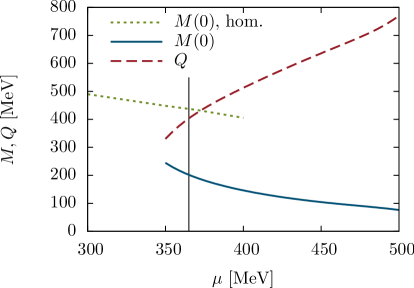
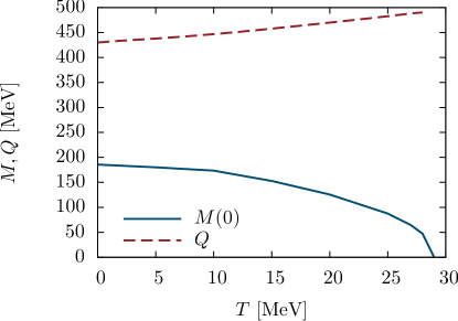
Figure 3: Mass amplitude $M(0)$ and wave number $Q$ as functions of $\mu$ at $T=0$ (top) and of $T$ at $\mu=370$ MeV (bottom). In the upper panel, the position of the first-order phase transition is indicated by the thin vertical line.

We now take the infinite-volume limit as specified in Eq. (4) and solve Eqs. (3) and (13) numerically. Results for the mass amplitude $M(0)\equiv B(\vec{0},n=0)/C(\vec{0},n=0)$ and the wave number $Q$ are presented in Fig. 3. In the upper panel we show them for $T=0$ as functions of $\mu$. At low chemical potential, we only find a homogeneous solution, whereas above $\mu=350$ MeV, there is also an inhomogeneous solution. Comparing the pressure, we find that the inhomogeneous phase becomes favored above a critical chemical potential of about 365 MeV. At this point a first-order phase transition takes place, where the wave number jumps from zero to a finite value, while the mass amplitude drops discontinuously, but remains nonzero. When we increase the chemical potential further, the latter continues to decrease, but with decreasing slope, suggesting that the inhomogeneous phase survives up to arbitrarily high chemical potentials. In fact, within numerical accuracy, we never find the chirally restored phase to be favored at $T=0$.

The lower panel shows the same quantities at $\mu=370$ MeV as functions of temperature. At this chemical potential the system is inhomogeneous at low temperatures, as evident from the nonvanishing $Q$. With increasing temperature, $Q$ increases further, while the mass continuously decreases and becomes zero at about $T=29$ MeV, where a second-order phase transition to the restored phase takes place.

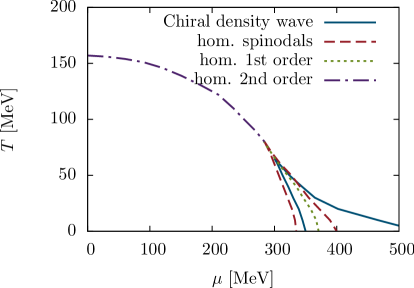
Figure 4: Phase diagram in the $\mu-T$ plane. The blue solid line indicates the boundaries of the region where the inhomogeneous solution exists.

Collecting the results from different temperatures and chemical potentials we obtain the phase diagram displayed in Fig. 4. At high temperature there is a second-order phase transition between the homogeneous chirally broken phase and the chirally restored phase (purple dash-dotted line), which becomes first order at low temperatures (green dotted line) when the analysis is restricted to homogeneous phases. The corresponding spinodals are indicated by the red dashed lines.

The limits of the region where we find an inhomogeneous solution with our CDW ansatz are marked by the blue solid lines. It can be deduced from the behavior of $\frac{d\Gamma}{dQ}(Q)$ that in this region the inhomogeneous phase is always favored over the restored phase. The restored phase is eventually reached in a second-order phase transition. Moreover, from the fact that the homogeneous chirally broken phase is energetically degenerate with the restored phase along the green dotted line, we conclude that the phase transition from the homogeneous to the inhomogeneous chirally broken phase must be to the left of this line. As already seen for $T=0$, this phase transition is first order. Hence, the phase boundary must be somewhere between the left solid and the dotted line. To locate it more precisely, we have to compare the pressure of the two solutions, which is numerically quite demanding. Within numerical precision we find that at $T=0$ the critical chemical potential is about 10 MeV lower than in the homogeneous case.

Our most important result is that, within numerical resolution, the inhomogeneous phase covers the first-order phase boundary of the homogeneous case completely. Moreover, the point where the inhomogeneous phase and the two homogeneous phases meet seems to coincide with the homogeneous critical point. In this respect, Fig. 4 has great similarities with the phase diagram in the Nambu–Jona-Lasinio (NJL) model  [18]. A qualitative difference is that in the NJL model the inhomogeneous phase ends at some upper critical chemical potential, whereas in the present case it seems to extent to arbitrarily high $\mu$ at $T=0$.

On the other hand, at high densities inhomogeneous chiral symmetry breaking should become disfavored against quark pairing (color superconductivity) [16], which we have neglected here. We have recently studied color superconductivity in a similar framework [19] and it should be a feasible task to extend the present analysis in this direction. Additionally it needs to be checked if the results of this work are robust under the improvement of the truncation. The consideration of more complicated inhomogeneous structures than the CDW ansatz would be interesting but extremely difficult as the propagator can no longer be inverted analytically.

References

- [1] P. Braun-Munzinger and J. Wambach, Rev.Mod.Phys. 81, 1031 (2009).
- [2] K. Fukushima and T. Hatsuda, Rept.Prog.Phys. 74, 014001 (2011), arXiv:1005.4814 [hep-ph].
- [3] Wuppertal-Budapest Collaboration, S. Borsanyi et al., JHEP 1009, 073 (2010), arXiv:1005.3508 [hep-lat].
- [4] A. Bazavov et al., Phys.Rev. D85, 054503 (2012), arXiv:1111.1710 [hep-lat].
- [5] M. Asakawa and K. Yazaki, Nucl.Phys. A504, 668 (1989).
- [6] C. S. Fischer and J. A. Müller, Phys.Rev. D80, 074029 (2009), arXiv:0908.0007 [hep-ph].
- [7] C. S. Fischer, A. Maas, and J. A. Müller, Eur.Phys.J. C68, 165 (2010), arXiv:1003.1960 [hep-ph].
- [8] C. S. Fischer, J. Lücker, and J. A. Müller, Phys.Lett. B702, 438 (2011), arXiv:1104.1564 [hep-ph].
- [9] C. S. Fischer and J. Lücker, Phys.Lett. B718, 1036 (2013), arXiv:1206.5191 [hep-ph].
- [10] W. Broniowski, Acta Phys.Polon.Supp. 5, 631 (2012), arXiv:1110.4063 [nucl-th].
- [11] A. Migdal, Phys.Rev.Lett. 31, 257 (1973).
- [12] F. Dautry and E. Nyman, Nucl.Phys. A319, 323 (1979).
- [13] W. Broniowski, A. Kotlorz, and M. Kutschera, Acta Phys.Polon. B22, 145 (1991).
- [14] E. Nakano and T. Tatsumi, Phys.Rev. D71, 114006 (2005), arXiv:hep-ph/0411350 [hep-ph].
- [15] D. Deryagin, D. Y. Grigoriev, and V. Rubakov, Int.J.Mod.Phys. A7, 659 (1992).
- [16] E. Shuster and D. Son, Nucl.Phys. B573, 434 (2000), arXiv:hep-ph/9905448 [hep-ph].
- [17] D. Nickel, Phys.Rev.Lett. 103, 072301 (2009), arXiv:0902.1778 [hep-ph].
- [18] D. Nickel, Phys.Rev. D80, 074025 (2009), arXiv:0906.5295 [hep-ph].
- [19] D. Müller, M. Buballa, and J. Wambach, Eur.Phys.J. A49, 96 (2013), arXiv:1303.2693 [hep-ph].