Chirally motivated separable potential model for amplitudes
Abstract
We analyze the interaction using a coupled channel separable potential model that implements the chiral symmetry. The model predicts an stattering length fm and in-medium subthreshold attraction most likely sufficient to generate -nuclear bound states. The energy dependence of the amplitude and pole content of the model are discussed. An idea of the same origin of the baryon resonances and is presented.
keywords:
chiral model , eta-nucleon amplitude , baryon resonancesPACS:
11.80.Gw , 12.39.Fe , 12.39.Pn , 14.20.Gk1 Introduction
A modern treatment of meson–baryon interactions at low energies is based on chiral perturbation theory (PT) that implements the QCD symmetries in its nonperturbative regime. The idea can be traced back to the late 1970’s when Weinberg came up with his phenomenological Lagrangians [1], the effective field theories which have a virtue in providing us with a systematic way to calculate the perturbative corrections. Being of this nature the PT has proven itself as an effective theory that utilizes an expansion in powers of small momenta and light quark masses. Naturally, the theory is expected to work well in the SU(2) sector due to smallness of the up and down quark masses. Interestingly, an extension to the SU(3) sector [2] has lead to a very successful description of interactions despite much larger mass of the strange quark and presence of the resonance just below the threshold [3], [4]. There, the PT is helped by a classical resummation technique, the Lippmann-Schwinger equation, which enables to sum up the major part of the perturbation series. As a result the higher order corrections are accounted for in a situation when the standard perturbation approach does not converge.
In the pioniering works [3], [5] the authors introduced local and separable potentials that match the chiral meson-baryon amplitudes up to a given perturbation order. The range parameters that appear in such approach do not only help to regularize the intermediate state Green function integral but they also provide a natural off-shell extrapolation of the amplitudes. This feature makes the model suitable for in-medium applications, particularly for a construction of meson-nuclear optical potential. We have followed this path in our recent works [6], [7] to establish a microscopical understanding of antikaon iteractions with nuclei.
Another way to manage the meson-baryon interactions reflects the unitarity of the scattering S-matrix and is based on a dispersion relation for the inverse of the T-matrix or on the N/D method [4], [8], [9]. There, the intermediate state Green function is regularized by standard quantum field techniques, most commonly by dimensional regularization. Both approaches lead to equivalent description (compare e.g. the two most recent analysis [7] and [10], both including the precise kaonic hydrogen data from the SIDDHARTA collaboration [11]) of the energy dependence of the meson-baryon amplitudes with the subtraction constants introduced in dimensional regularization non-trivially related to the range parameters employed in the potential model.
The chiral coupled channels approaches to interaction have brought quite new insights on the dynamics of the meson baryon interactions in the free space as well as in the nuclear medium. One of the most interesting results appears to be the two-pole character of the resonance [9] which is formed dynamically due to a strong inter-channel coupling in the – system [12]. The dynamics of the then leads to a strong energy dependence of the amplitude not only in the free space but in nuclear matter as well [13], [7]. It has been well known for some years that the -nuclear optical potentials constructed from the chirally motivated amplitudes taken at the threshold energy are quite shallow [14], [15] while a phenomenological analysis of kaonic atoms revealed very attractive deep -nuclear potentials [16]. It was demonstrated in Ref. [13] that these two conflicting scenarios can be reconciled by considering properly the subthreshold energy dependence of the amplitude. Indeed, it appears that the relatively weak attraction becomes much stronger at energies about 30-50 MeV below the threshold that are probed by antikaons in nuclear matter, although even more attraction is needed phenomenologically. This strong attraction is also in agreement with predictions by relativistic mean field theories that implement the antikaon field [17]. It comes without saying that a good understanding of (anti)kaon interaction with nuclei would not be possible without realistic models to describe the subthreshold energy dependence of the amplitudes in the free space as well as in the nuclear medium. The potential we used to study the interactions perfectly suits this role.
The situation is quite similar in case of the interaction whose energy dependence around the threshold is also strongly affected by a resonance, this time the one. Thus, it seems natural to utilize the techniques developed for the system and apply them to the one. This is exactly what represents the content of our current work. In close resemblance to our model [6], [7], here we study the system within a chirally motivated coupled channels framework. In fact, the same approach was already used in Refs. [5], [18] and [19] though the authors of those works restricted their analysis to a relatively narrow energy interval above the threshold. We are also in a more favourable position thanks to new precise data on the reaction [20] as well as due to an existence of a more advanced database of the partial waves [21]. We note that the interaction was also recently studied by other authors who used the unitary coupled channel approach based on solving the Bethe-Salpeter equation [22], [23] and [24]. Excepting Ref. [22] these models predict a moderately attractive interaction with a scattering length fm while a considerably larger attraction was obtained in -matrix fits to and reaction data with fm [25]. As we will show, our model yields fm, a value approximately in-between those two estimates and in agreement with Refs. [5] and [22]. Naturally, the strength of the attraction at the threshold and at energies below the threshold are relevant for a possible existence of -nuclear bound states [26]. The authors of Ref. [26] found that an attraction related to fm might be just sufficient to generate -nuclear bound states in the 24Mg isotope (and in heavier targets) while a stronger attraction is required for binding the in lighter nuclear systems.
The paper is organized as follows. After a brief introduction of the model in Section 2 we detail the procedure to fit the model parameters and our treatment of the experimental data in Section 3. In Section 4 we make comparisons with approaches by other authors and present the results of our own fits. The section is also continued with a discussion of the energy dependence of the amplitudes in the free space. Finally, in Section 5 we examine the pole content of the model and its relevance to the and resonances. The paper is closed with a short Summary.
2 Coupled channel chiral model
The meson-baryon effective potential employed in our work is given in a separable form
| (1) |
with the off-shell form factors chosen in the Yamaguchi form,
| (2) |
Here the indexes and run over the coupled meson-baryon channels and we number them in order of their threshold energies. Further, () represents the CMS meson-baryon momenta in the initial (final) state, stands for the two-body CMS energy, and the inverse ranges characterize the interaction range of the specific meson-baryon states. The central piece of the chirally motivated potential matrix reads
| (3) |
where is the meson decay constant and denotes the baryon mass in the -th channel. Following the approach of other authors [22], [23], [10] we (in principle) allow for different values of that relate to the specific meson appearing in the -th channel.
The coupling matrix is energy dependent and its form is determined by the chiral SU(3) symmetry. At the leading order Tomozawa-Weinberg (TW) interaction it is given as
| (4) |
with the TW couplings standing for the standard SU(3) Clebsch-Gordan coefficients. In our work we also take into account the next-to-leading order (NLO) contributions to the matrix that contribute at the order of the external meson momenta. The relation to a chiral expansion in terms of small meson momenta and quark masses is guaranteed by matching the pseudopotentials Eq. (3) to the meson-baryon amplitudes evaluated within the PT to a given order, see Refs. [3], [6] for details. In Born approximation and for the momenta on the energy shell the meson-baryon amplitudes are equivalent with the pseudopotentials defined by Eq. (3). Thus, a positive sign of the pseudoponetial (or a negative sign of the pertinent diagonal coupling ) corresponds to an attractive interaction in the -th channel. We also note in passing that a slightly different energy dependence of the TW term was used in some of our earlier works based on the heavy baryon formulation of the underlying chiral Lagrangian. The form adopted here and defined by Eq. (4) reflects the fact that physical baryon masses do differ from a common baryon mass in the chiral limit.
As we already stated the contributions included in our inter-channel couplings reflect the structure of the underlying chiral Lagrangian. Instead of writing up all the pieces that appear in the Lagrangian at the first and second chiral orders (for details see e.g. Refs. [3], [27]) we illustrate the contributions relevant for an -wave scattering in a form of Feynman diagrams shown in Figure 1. The first diagram visualizes the already mentioned current algebra TW term that plays a major role for the meson-baryon interactions at low energies and some analysis restrict themselves to only this interaction. The direct s-term and crossed u-term represent Born amplitudes that also originate from the first order chiral Lagrangian. When expanded in terms of external meson momenta the first three diagrams include not only the order but give also rise to relativistic corrections of the and higher orders. In addition we also incorporate the NLO terms from the second order chiral Lagrangian that are represented by the contact diagram shown as the last one in Fig. 1. These contributions can be viewed as NLO corrections to the TW term. The exact form of all contributions related to the depicted diagrams, that we use to build the coupling matrix , as well as the involved parameters (low energy constants) of the model are specified in the Appendix.

The separable potentials defined by Eqs. (1) and (3) are then used in the Lippmann-Schwinger equation that allows us to solve exactly the loop series and obtain the meson-baryon amplitudes in a separable form as well,
| (5) |
The algebraical solution for the reduced (stripped off the form factors) amplitudes then reads
| (6) |
with an intermediate state meson-baryon Green function
| (7) |
Here we assume that the interaction occurs in a free space which also allows us to perform the analytical integration in Eq. (7). The impact of nuclear medium can be implemented easily in the model with the transition amplitudes (6) acquiring a density dependence [13], [7]. In such a case, the Green function (7) would also become density dependent with the free space propagator modified due to Pauli blocking [28] and by the meson and baryon selfenergies [29].
The dynamics of the system is defined by the involved meson-baryon channels and by the inter-channel couplings derived from the PT. In the present work we apply the model to study the interactions and include all the channels that represent the interactions of the lightest meson octet with the lightest baryon octet. For practical reasons we will work in the isospin basis of states and treat separately the channels with isospins and . Thus, we have four coupled channels (, , and ) and two channels ( and ). Although we aim exclusively at the interaction that is restricted to the isospin the channels are involved in fits of the free parameters of the model. In both sectors the channels are ordered according to the channel threshold energies. We assign the channel indexes in the just specified order, reserving the first four indexes to the channels and indexes to the channels. This allows for a compact analysis with only one coupling matrix that is specified completely in the Appendix. Of course, one could also work with six physical charged channels (, , , , , ) which would allow for a proper treatment of threshold effects. However, as we intend to match the experimental data on the amplitudes that are presented as partial waves with a well defined isospin and the state itself has also a well defined isospin, we feel that doing the analysis in the isospin states basis is more appropriate. If a need arises the model can easily be adapted to work with the physical meson-baryon states too.
3 Fits to experimental data
The chirally motivated potential model described in the previous section has quite many parameters that have to be either fixed by making reasonable assumptions or fitted to the available experimental data. First of all there are the meson weak decay constants which we fix at their physical values MeV, MeV and MeV [2], depending on the meson in the respective channel. The strengths of the direct and crossed Born terms are characterized by combinations of the axial vector coupling constants and with the commonly accepted values taken from an analysis of semileptonic hyperon decays [30]. The -couplings of the NLO contact terms and the common baryon mass were fixed in Refs. [31] and [6] to satisfy the Gell-Mann formulas for baryon mass splittings and to guarantee a chosen value of the pion-nucleon sigma term . Further, there are four independent -couplings that determine the strengths of the double derivative contributions to the NLO contact terms, to the last diagram of Fig. 1. These four parameters and the inverse ranges that characterize the Yamaguchi form factors, Eq.(2), are left free to be fitted to the experimental data. In summary, we are left with eight free parameters, four -couplings and four inverse ranges .
To perform the fits we use the MINUIT routine from CERNLIB to minimize the per degree of freedom defined as
| (8) |
where is the number of fitted parameters, is a number of observables, is the number of data points for an -th observable, and stands for the total computed for the observable. Eq. (8) guaranties an equal weight of all fitted data.
There is a plenty of experimental data on low energy scattering and reactions. The model parameters are fitted to
-
1.
amplitudes for the and partial waves taken from the SAID database [21]
-
2.
selected reaction total cross section data
Primarily, we make use of a comprehensive analysis of the available data and match our -wave amplitudes in the and partial waves to those from the SAID database [21]. Taking into account the normalization of the SAID amplitudes this is done by multiplying our amplitude , Eq. (5), by the magnitude of the CMS momentum in the initial channel,
| (9) |
where we refer explicitly to a given partial wave. Since we are interested mainly in the low energy region close to the threshold and up to about MeV subthreshold we restrict ourselves to meson-baryon CMS energies below MeV. In the energy interval from the threshold up to MeV there are 30 single energy data points for each of , , , . Considering the precision of the SAID analysis and comparing it with a previous one by the Karlsruhe-Helsinki group [32], we follow the approach of Ref. [24] and assume a semiuniform absolute variation of the SAID amplitudes. This variation is set to fm for energies below 1228 MeV, and to fm for energies above 1228 MeV. Finally, it is apparent in the SAID analysis that the experimental amplitude is srongly affected by the resonance at the higher end of our energy interval. Since this resonance does not have a prominent dynamically generated component and is completely missing in our model we exclude the affected amplitudes from our fits. A comparison of the amplitudes generated by our model with those from the SAID analysis has shown that we can safely consider the SAID data in the sector up to MeV. This means that for the and amplitudes we exclude from the fit the SAID data at 9 highest single energies.
In addition to the amplitudes we also fit the reaction cross sections. In our formalism, the total -wave cross sections for a transition from -th to -th channel, are given by the standard formula,
| (10) |
In the isospin basis, the experimental production cross section can be identified with calculated within our coupled channels model. There are very precise experimental data on the production from a recent measurement by the Crystall Ball collaboration [33]. The precision of these data exceeds by far the much older data from previous experiments. For this reason we consider only the new data from Ref. [33] in the energy region above the threshold and complement them with data from three other older measurements [34], [35], [36] only at energies above MeV, the highest energy treated in Ref. [33]. In accordance with our approach to the amplitudes we also restrict ourselves to energies below MeV. This means that a -wave contribution to the fitted total cross sections can be neglected. However, to match properly the experimental production data we modify the calculated cross sections to account for a lack of the three-body channel in our model. This channel decreases the experimental inelasticity of the amplitude reported in the SAID database. The total reaction cross section reads as
| (11) |
The SAID database provides a factor at the energy MeV which gives a total reaction cross section of about mb, approximately 20% larger than the maximum of the experimental cross section. In our fit procedure we effectively compensate for the missing channel by enhancing the calculated cross sections that represents in our model the only reaction channel which is open in the discussed energy region. Thus, the calculated cross section is matched to the experimental one by using a relation
| (12) |
We note that an introduction of the factor of is in agreement with observations made in Ref. [37]. We also found that fits made without this factor lead to only slightly worse reproduction of the production data while the effect on the overall quality and other characteristics of the fit is not significant.
4 Results
4.1 The KSW model
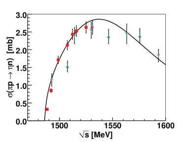
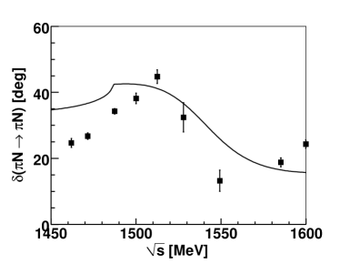
Before presenting the results of our fits to the experimental data we check the functionality of the model and the pertinent computer code by reproducing the old results by Kaiser, Siegel and Weise [5]. They used essentially the same effective meson-baryon potentials with an alternate energy dependence of the TW term and omitted contributions from the Born diagrams, the direct and crossed terms shown in Figure 1. The two Born diagrams were included in a following work [18] in which the authors got an equivalent description of the data. However, a comparison of these later results with our current work is not so straightforward due to a different form of the off-shell form factors employed in Ref. [18]. In what follows we will refer to the original model of Ref. [5] by the KSW tag and use it for a comparison with our own fits. Adopting the KSW potential form and parameters of the KSW model we were able to reproduce nicely their results. They are shown in Figure 2 which is to be compared with Figure 1 and with the left panel of Figure 2, both of them published in Ref. [5]. The experimental data on the production are taken from Refs. [33], [34], [35] and [36]. The first three data points marked by triangles in our Figure 2 were not included in our fits and are given in the figure to show the superiority of the recent experimental data over the older ones at energies closely above the threshold. The experimental data on the phase shifts are taken directly from the SAID database [21].
Concerning a comparison of the KSW model with our own fits one should remember that the KSW model was designed to reproduce the experimental data only in a relatively narrow region of the resonance, in an interval limited to the CMS energies MeV MeV. We found that the amplitudes generated by the model start to deviate quite significantly from those of the SAID analysis as soon as one goes below the threshold. Thus, the KSW model is clearly not suitable for description of the and data in the whole energy region MeV considered here.
4.2 New fits and results
The results of our fits are shown in Table 1 in comparison with the KSW model. To have some variety and check a consistency of our model predictions we opted for three different choices of the pion-nucleon sigma term that fixes the parameter and the common baryon mass in the chiral limit. Specifically, we adopt the values , and MeV and use the respective number when tagging the NLO models. The choice MeV was also used in our CS30 and NLO30 models applied to the system and discussed in [7]. To distinguish the model notation from our previous works we add a subscript for our present models fitted to the related data. As we see from Table 1 all three fits give a comparable level of data reproduction with the model NLO20η reaching only slightly better value of that the NLO30η model. We also tried to perform the fits without restricting the energy region for the amplitudes (to energies below MeV) and without accounting effectively for the channel (a factor 1.2 in the production cross section). With the parameters fixed to we got then. This value drops significantly to 1.69 when we exclude the data affected by the resonance from the fit. A further improvement from 1.69 to the 1.46 reported for the NLO30η model is due to the effective accounting of the channel. Thus, we conclude that our treatment of the experimental data is reasonable and leads to their consistent reproduction.
| model | |||||||||
|---|---|---|---|---|---|---|---|---|---|
| NLO20η | 1.33 | 597 | 1293 | 256 | 1032 | 2.062 | -0.896 | -2.279 | 3.528 |
| NLO30η | 1.46 | 538 | 1635 | 250 | 939 | 1.981 | -0.770 | -2.452 | 3.940 |
| NLO40η | 1.95 | 508 | 2000 | 250 | 842 | 1.863 | -0.685 | -2.608 | 4.366 |
| KSW | — | 573 | 776 | 776 | 776 | 0.420 | -0.410 | -0.745 | -0.380 |
Concerning the KSW model we emphasize that the model is included in Table 1 only for a reference and comparison of the fitted parameters. The pertinent value of is omitted in Table 1 since a direct comparison with the values of our new fits is not meaningful. This is because not only the data set was different in [5] from the one used here but a number of the fitted parameters and a number of observables were different in Ref. [5] too. As anticipated we checked that the KSW model leads to unacceptably large when calculated with the present fitting metodology applied to the whole energy interval starting from the threshold.
It is worth noting the differences in the fitted parameters. All our three models lead to a inverse range MeV in good agreement with the KSW value. Our models are characterized by very large inverse range in the channel making the system quite compact. The opposite can be said about the channel while a moderate value of MeV resulted for the channel. We have no explanation for such vast differences between the involved meson-baryon systems. Though, in average our results are in line with a common value of the inverse range used for the three nonpionic channels in the KSW model.
The -couplings obtained in our fits and shown in Table 1 are quite large and completely at variance with the KSW model, that attempted to keep them close to those from studies [3] made earlier by the same authors, and with our own previous studies of the system [6], [7]. In principle, it seems natural to assume a common low energy constants for both and strangeness sectors. However, as the -couplings are the only Lagrangian couplings that are left free in our model, parts of them effectively make up for all contributions that are not accounted for at the NLO level. The higher order corrections omitted at the NLO level are different in the and sectors and apparently more important in the sector than in the one. In other words, the large values of our -couplings indicate a worse convergence of the in the sector. This is also reflected by a commonly accepted observation that the chiral expansion works reasonably well for the system already at the LO order, at least in the energy region around the threshold. On the contrary, we have found that we could not achieve a satisfactory description of the and experimental data without introducing the NLO terms. We have also made an attempt to vary only the inverse ranges while fixing the -couplings to those established in our previous NLO30 fit to the data. The resulting is not acceptable and clearly indicates that the and data are difficult to describe with a common set of low energy constants at the NLO level. The achievement of Ref. [3] is a bit misleading in this sense as we found that the applicability of the KSW model is restricted only to a narrow interval of energies above the threshold. We also note that quite different NLO couplings for the and sectors were obtained in separate fits to the pertinent data by another group of authors in Refs. [24] and [38], respectively. Of course, it would be best if a simultaneous fit to both the and related data were attempted to find out whether a common set of LECs exists for both sectors (as unlikely this might seem), but this goes beyond the scope of our present work.
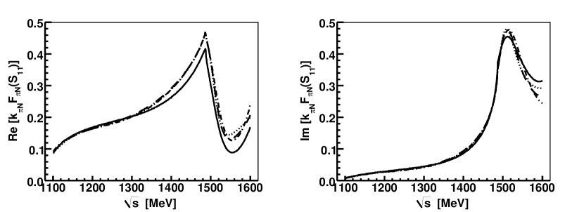
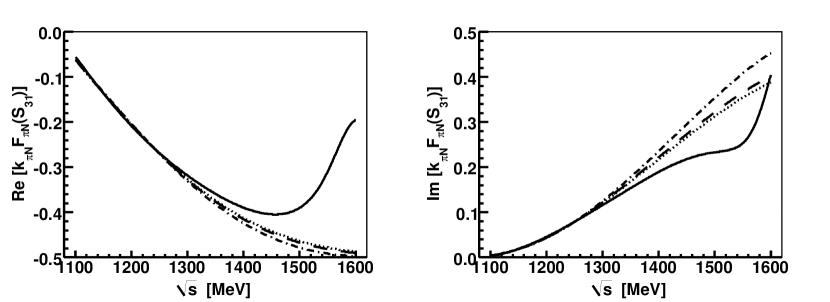
In Figure 3 we demonstrate how well our models reproduce the -wave amplitudes from the SAID database. In the whole energy region all three models give equivalent amplitudes with hardly noticeable differences among them, especially below the threshold. The overall reproduction of the SAID amplitudes is quite good for the partial wave. Deviations from the SAID amplitudes observed for the amplitude at higher energies are caused by the resonance (which is not accounted for in our model) and justify our omission of the affected data from the fits. We note that much larger variance between the calculated and SAID amplitudes is obtained when only the TW term is used in the effective meson-baryon potentials, see e.g. Fig. 2 in Ref. [23]. On the other hand, the quality of the fits performed in Ref. [24] seem to be slightly better than ours, though the authors fitted a bit different set of experimental data and varied a larger number of model parameters. A qualitative comparison of predictions for the amplitudes made in the current work and in Ref. [24] with those of Ref. [23] once again demonstrate the importanance of the NLO interaction terms, specifically at low energies between the and thresholds.
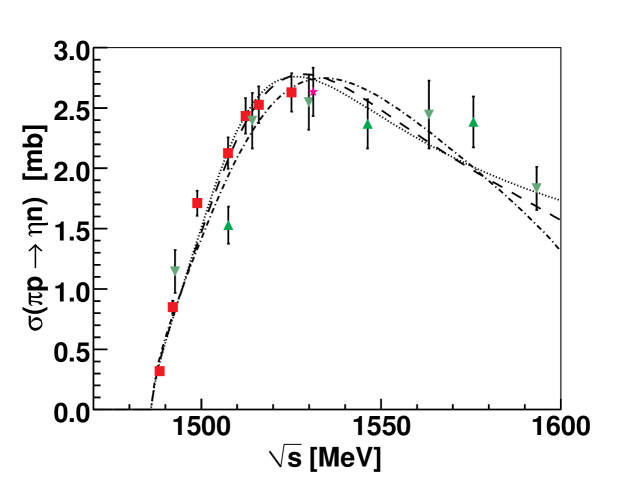
In Figure 4 we present the calculated total cross sections in comparison with the experimental data, the same ones as in Figure 2. The agreement of the theoretical predictions with the experimental cross sections is quite good for all three models. The models give very similar results for energies up to about 1580 MeV, then start to deviate. Apparently, a fit to higher energy data would be necessary to make distinction among them. However, this would require an introduction of higher partial waves and a proper treatment of the channel, tasks that go beyond restrictions of the present approach.
The peak structure of the production cross section relates to the resonance and is nicely reproduced by our models. We have also noted that the peak position is closely related to the compactness of the system resulting from our fits. When we fixed the inverse range at a smaller value (e.g. at 700 MeV) and fitted the remaining model parameters we were able to achieve a reasonably good overall agreement with the experimental data, though only on the expense of moving the production maximum to higher energies, about 30 MeV off the one seen in Figure 4. We will come back to this feature when discussing the position of a pole related to the resonance in Section 5.
4.3 amplitudes
The energy dependence of the elastic amplitudes is visualized in Figure 5. All our three NLO models lead to very similar predictions for the amplitudes, at some parts difficult to distinguish one from the other. This is in contrast to the predictions of the KSW model that lead to a smaller attraction at the threshold and to much larger imaginary part of the amplitude below the threshold. The scattering lenghts generated by the NLO30η and the KSW models are fm and fm, respectively111The scattering length reported in Ref. [5] is fm having a real part at variance with our reproduction of the KSW results. Most likely, the value given in Ref. [5] refers to their local potential, not to the KSW separable potential we reproduce and compare with here.. Our values are also significantly larger than most of other predictions by chirally motivated models [5], [18], [23], [24] and closer to the value of fm established in -matrix analyses of the and reaction data [25], [39], [40]. A similar value of fm, quite close to our result, was obtained in Ref. [22].
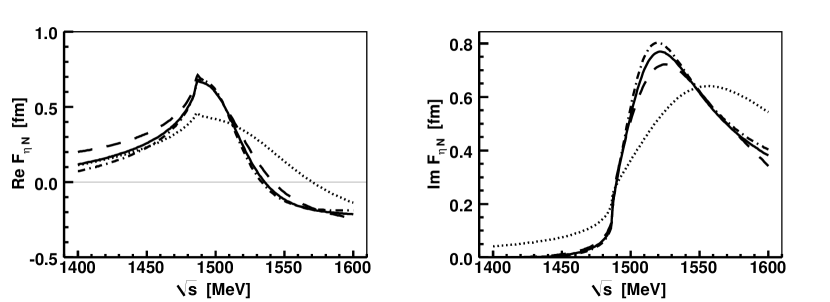
As we already mentioned in Section 1 the strength of the threshold (and subthreshold) attraction was discussed in Ref. [26] in relation to a possible formation of the -nuclear bound states. There, the authors found that the attraction provided by models that generate fm is not sufficient for forming the -nuclear bound states in the lightest nuclei including . Taking into consideration their results we estimate that our model attraction might be just sufficient to form the nuclear bound states from on. However, a proper in-medium treatment of the interaction requires a shift of the interaction energy to the subthreshold region as well as introduction of hadron selfenergies in the intermediate state propagator. The first effect was accounted for in Ref. [26] while an impact of the latter one is studied in another work prepared for publication [41]. The in-medium dressing of hadrons was also considered in an earlier work by Inoue and Oset [42] who reported an increased in-medium -nuclear attraction at subthreshold energies. Although our own preliminary findings do not comply with their observations in this respect it is quite clear from both works, the [41] and [42] ones, that a proper treatment of the -nuclear interaction depends on a reliable extrapolation of the interaction to subthreshold energies. In this sense, it is incouraging to note a good agreement (at least for the real part of the amplitude) at the subthreshold energies between our three models and the KSW one.
Our models predict a very sharp drop of the imaginary part of the amplitude at the subthreshold energies. In Figure 5 we see that the KSW model leads to significantly larger there. However, as the KSW model does not reproduce well the amplitudes at energies below the threshold we maintain that our results are more realistic within the model constrains. The small implies a small absorptivity of the -nuclear optical potential. Though, one should also remember that models discussed here lack completely the three body channel. Its introduction should lead to a larger imaginary part of the elastic amplitude and to a related increase of the imaginary part of the optical potential. In close resemblance to -nuclear studies [43], [44] we also expect contributions to the optical potential, to both its real as well as imaginary parts, arising from meson interactions with nucleon pairs (and clusters in general).
5 Dynamically generated resonances
In Table 2 we show the positions of the poles our models generate on two Riemann sheets that are connected with the physical region in the considered energy interval. The Riemann sheet (RS) connected to physical region by crossing the real axis between the and thresholds is denoted as [-,-,+,+] with the signs marking the signs of the imaginary parts of the meson-baryon CMS momenta in all four coupled channels (unphysical for the and channels and physical for the and ones). Similarly, the RS connected with physical region in between the and thresholds is denoted as [-,-,-,+]. We note that all three models give very similar predictions for the pole that can be assigned to the resonance. The position of the pole is not so well determined by our models. For the NLO20η and NLO30η models we find the pole on the RS reached by crossing the real axis above the threshold but the pole itself lies below it. Even then, it is still the pole that is closest to the physical region for energies above the threshold. For this reason it is natural to assign it to the resonance which was reported as a dynamically generated state in other chirally motivated coupled channels approaches to the system [22], [24]. The difference between and the experimentally established peak position of the resonance can be explained by two factors. First of all the pole energy is shifted with respect to the peak energy due to an interference with background, similarly as it is so for the pole . Secondly, our models are based exclusively on the experimental data for energies below 1600 MeV. Thus, any model predictions for higher energies may be very unprecise quantitatively. It is also interesting to note that the pole positions of both poles reported in Table 2 show a trend of increasing the pole energies (the real as well as imaginary parts) with the value of the term the model parameters are fixed to. Considering a possible shift of the pole to lower energies with respect to the cross section peak position, one can deduce that for MeV the pole would be at about right place for an assignment to the resonance.
| model | [MeV] | [MeV] |
|---|---|---|
| NLO20η | 1502 - i33 | 1548 - i39 |
| NLO30η | 1503 - i37 | 1579 - i81 |
| NLO40η | 1504 - i48 | 1631 - i167 |
| PDG [45] | 1510 - i85 | 1655 - i70 |
When comparing our pole positions with the pole estimates by the Particle Data Group (PDG) [45] one should keep in mind model ambiguities related to extending the resonance properties determined in various experiments to the complex energy plane. In Table 2 we give only the average PDG estimates while the complete PDG listings provide pole positions determined by various authors that cover relatively broad region of energies around the PDG averages. The positions of our pole are in nice agreement with the PDG listings for the with the imaginary part provided by our NLO models at about the lower boundary of model predictions by other authors. Unfortunately, the same cannot be said about our predictions for the pole, most likely due to reasons we gave above.
The origin of resonances generated dynamically due to couplings between various meson-baryon channels can be traced to existence of poles in the zero coupling limit (ZCL), a hypothetical situation in which all inter-channel couplings are set to zero and the poles may persist only in those single channels that have nonzero diagonal couplings [46], [47]. This is also a case for the resonance which appears to be composed of two very close resonances, one of them related to a bound state in the channel, the other to a resonance in the channel. There, the - inter-channel dynamics move the poles from their positions in the ZCL to those predicted by the models in the physical limit [12], [48]. The situation is similar in the strangeness sector for the isospin where only the and channels have nonzero diagonal couplings. Since the threshold is too far below the one we anticipate that the dynamically generated poles and emerge from the system. Indeed, this is a case as we demonstrate in Figure 6 made with the NLO30η model. The diagonal coupling is strong enough to generate a virtual state at an energy about 70 MeV below threshold. In the ZCL this gives us a pole position at the real axis on a RS that is unphysical in the channel. As soon as the inter-channel couplings switch on this pole departs from the real axis and can start moving on any of the Riemann sheets that keep the minus sign for the channel. In Figure 6 we follow the movements of the poles on the Rieman sheets [+,+,-,-] (continuous line, pole) and [+,+,+,-] (dashed line, pole) in the upper half of the complex energy plane. The pole trajectories show the pole positions as we gradually increase a scaling factor that is applied to the non-diagonal inter-channel couplings from (zero couling limit) to (physical limit). The dots mark the positions of the poles for , , …, with the last point showing the final pole positions at full physical couplings, those given in Table 2 for the NLO30η model. The figure demonstrates that both poles, and , evolve from the same origin and that they are mutually shadow poles. For small values of the scaling factor the pole positions on both Riemann sheets remain very close to each other and the two trajectories are hard to separate. The trajectories cross the real axis at energies above the highest meson-baryon threshold, so the poles continue their movements in the lower part of complex energy plane on Riemann sheets with all the signs reversed, the pole on the [-,-,+,+] RS and the pole on the [-,-,-,+] RS. In this part of the figure the trajectories are already clearly separated and the final pole positions for (in the physical limit) are quite different.
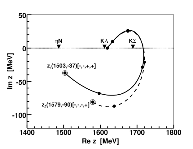
To complete our analysis of pole movements from the ZCL we add that there are also shadow poles which emerge on the [+,-,+,-] and [+,-,-,-] Rieman sheets for small values of . Their trajectories cross the real axis twice, first about 10 MeV below the threshold, then again immediately above the threshold, so the poles evolve on the [+,-,+,+] and [+,-,-,+] Rieman sheets for , respectively. The final positions of those poles for are at the energies MeV on the [+,-,+,+] RS and at MeV on the [+,-,-,+] RS. Though the energies are in agreement with and poles expectations, the [+,-,-,+] RS is too far from physical region for the pole to have any impact on physical observables. The pole on the [+,-,+,+] RS is relatively close to the threshold and not that far from physical region, but it plays only a secondary role to the pole on the [-,-,+,+] RS that is connected with the physical RS in between the and thresholds. Finally, we note in passing that no poles emerge from the ZCL on the other Rieman sheets (e.g. on the [-,-,-,-] RS) that are unphysical in the channel. Thus, the two pole trajectories depicted in Figure 6 are the only two that bring the poles to positions which are physically relevant.
We would like to point out that the model does not leave any room for more dynamically generated resonances with in the energy region above the threshold. If there is a resonance on any RS connected to the physical region in that area it must originate from the virtual state in the channel found in the ZCL. We checked that the other channel with nonzero diagonal coupling, the one, provides a resonance too far from the real axis which is not moved any closer due to inter-channel dynamics. Thus, provided that the resonances and are both generated dynamically, they should be viewed as two manifestations of only one substance that emerge as reflections of two shadow poles on two different Rieman sheets. The observable physical quantities (cross sections) are always affected by the pole that is closer to a given energy in the physical region (at the real axis), or that couples more strongly to a given physical state. It is also known that sometimes two shadow poles may have a comparable bearing on a physical observable, so both of them will affect it.
The pole positions can be found as solutions (for the complex energy variable ) of an equation that sets to zero the determinant of the inverse of the matrix, [48]. In the ZCL the condition for a pole in the -th channel is equivalent to solving an equation which leads to
| (13) |
This equation clearly shows that the position of the pole in the ZCL depends on the strength of the coupling and on the value of the inverse range that enters the expression for the form factor as well. This was already realized in Ref. [5] where a formation of a resonance state was linked to the magnitude of the range parameter, see Table 1 there. Our Eq. (13) provides a qualitative understanding of the relation. As the pole is moved from the ZCL due to inter-channel couplings the inverse ranges of the other channels get involved too and the situation becomes much more complicated. The final position of the pole in the physical limit is affected by many factors including the energy dependent inter-channel couplings , thus it is difficult to establish a clear link between the inverse ranges and a position of the pole. For the NLO30η model we checked numerically that the pole related to moves to higher energies and further from the real axis with a decreasing value of .
With the pole positions established one can also determine the couplings of involved channels to the pertinent resonant states. Here we follow Ref. [49] and express the transition amplitude in a vinicity of the complex pole energy as
| (14) |
where the non-resonant background contribution and the dependence of the resonant part on the on-shell momenta are shown explicitly. The symmetric matrix has rank 1 and the complex couplings can be determined from the residui of elastic scattering amplitudes calculated at the pole energy. They are related to the partial widths
| (15) |
that refer to the probability of the resonant state decaying into the -th channel. In reality, a resonant state can decay only into channels that are open at a given energy, so our Eq. (15) does not make a good sense for channels with thresholds much higher than the pole energy . However, in a case of a broad resonance (when the pole is not close to the real axis) the branching ratios calculated at the complex pole energy may differ significantly from the branching ratios established in experiment and assigned to the resonance peak energy. In addition, a tail of a resonance can also contribute to experimentaly measured branching ratio even in a situation when the pole energy (or a resonance peak) is found below the channel threshold. Finally, from the experimental point of view, it is very difficult (if not impossible) to establish the partial widths independently of a formation process that is particular for a given measurement. Thus, any theoretical partial widths calculated at the pole position are only approximately related to those established experimentaly. Keeping all that in our mind we have applied Eq. (15) not only to channels open at the pole energy but to the closed ones as well.
In Table 3 we present the unitless branching ratios defined as
| (16) |
When looking at the numbers in the table one notices that the standardly anticipated unitarity relation is sizebly violated, even when the summation index runs only over the open channels. In view of the ambiguities discussed above and because the peak of the resonance lies above the threshold we consider the channel as open for the pole, though the pole is located below the threshold for the NLO20η and NLO30η models. For both the and poles the sums of the open channels branching ratios differ from unity by as much as . However, in fact the relation should hold only for an isolated pole of the Breit-Wigner type and in absence of any background that would interfere with the resonance. There is no way to say whether the dynamically generated poles can be reliably approximated by the Breit-Wigner formula. Clearly, there is a background due to a distant presence of the pole related to the channel and the branch cuts at the real axis that open at the channel threshold have some effect too. Thus, it is not surprising that the discussed relation holds just approximately even if we sum only over the open channels. The large values of the partial widths reported for the closed channels do not have a physical meaning and they reflect large magnitudes of the pertinent complex CMS momenta . In fact, the effective couplings are of a natural size.
| pole | pole | |||||||
|---|---|---|---|---|---|---|---|---|
| model | ||||||||
| NLO20η | 0.33 | 0.70 | 7.92 | 11.4 | 0.40 | 0.26 | 0.14 | 8.27 |
| NLO30η | 0.36 | 0.73 | 19.9 | 16.7 | 0.35 | 0.15 | 0.15 | 4.46 |
| NLO40η | 0.41 | 0.82 | 35.5 | 26.5 | 0.81 | 0.19 | 0.21 | 6.75 |
| PDG [45] | 0.45 | 0.42 | — | — | 0.70 | 0.10 | 0.03 | — |
Similarly as for the pole positions we show only the PDG average estimates in Table 3 rather then the whole intervals reported by various authors and listed by the PDG [45]. As we already argued the branching ratios calculated from the amplitude residui at the pole positions may be quite different from the experimentaly determined ones. Thus, the comparison of our model predictions with the PDG estimates is presented here merely to illustrate how large the differences may be. It is still interesting to note the quite large BRηN predicted by our NLO models for the resonance. Besides the reasons stated above another factor influencing this may be related to an ommission of the decays in our model that are effectively accounted for by decays into the channel.
6 Summary
In summary, we have presented new fits of the and data for the partial -wave including CMS energies from the threshold up to MeV. The resulting chirally motivated meson-baryon potentials lead to the scattering length fm corresponding to much stronger attraction than generated by other chiral models. The separable character of our model with its natural off-shell extrapolation makes it suitable for in-medium applications, specifically for studies of possibly bound -nuclear states. The energy dependence of our amplitudes at subthreshold energies required in such studies is consistent with earlier predictions by other authors, though the imaginary part of our amplitude may fall too fast when going subthreshold. If the same feature was preserved for the in-medium amplitude, the predicted -nuclear bound states would have unrealistically small absorption widths. This effect arises due to a restriction of our model to two body interactions, particularly due to an omission of the channel, the only inelastic channel in induced reactions that opens below the threshold. We leave an implementation of the channel for a future.
In the discussed region of energies the - interactions are strongly affected by the and resonances, both of them generated dynamically by our model. We have found that both states have the same origin that can be traced to the virtual state, established on the real axis below the threshold on the unphysical RS when the inter-channel couplings are switched off.
In general, the present analysis of interactions compliments our earlier studies of the system which we did in the same coupled channels framework that relies on chiral dynamics. In both situations we have vitnessed a strong energy dependence of the elastic meson-baryon amplitudes at energies close to the threshold and particularly below the threshold. While the dynamics of the system is driven by the resonance the low energy interactions are strongly affected by the resonance. The discussions of both systems with the same methodology provide us with a better control of the related models and give us new insights on general aspects of meson-baryon interactions in the nonperturbative regime.
Acknowledgement
A. C. would like to thank E. Friedman and A. Gal for their warm hospitality and stimulating discussions during his stay at the Hebrew University in Jerusalem where part of the work was completed. The authors also acknowledge a help by R. Workman who provided us with the source data on the production icluded in the SAID database. The work of A. C. was supported by the Grant Agency of Czech Republic, Grant No. P203/12/2126.
Appendix
The central piece of our pseudopotentials Eq. (3) is the coupling matrix which form is derived from the SU(3) chiral symmetry and reflects the structure of the underlying chiral Lagrangian. Considering the leading and next-to-leading orders of the chiral expansion and making a projection to the -wave the couplings can be expressed in a form [3], [6], [7]
| (17) | |||||
where , and denote the meson mass, CMS energy and momenta in channel , respectively, and stands for the baryon mass in the chiral limit. The general structure of the coefficients follows closely the one we adopted in our earlier studies of the interactions [6], [7]. The terms marked by the superscripts ”WT” and ”u” correspond to the leading TW contact interaction and to the crossed Born amplitude represented by the diagrams a) and c) in Figure 1, respectively. The remaining parts contribute to the contact interaction in the next-to-leading order visualized by diagram d) in the figure. There, the last two terms on the third line in Eq. (17) represent an explicit breaking of the chiral symmetry (the “” term) and a violation of the Gell-Mann–Okubo formula (the “GOv” term).
| 2 | 0 | 0 | 0 | |||
| 0 | 0 | 0 | ||||
| 0 | 0 | 0 | 0 | |||
| 2 | 0 | 0 | ||||
| -1 | -1 | |||||
| -1 |
The reader may wonder why a direct Born term represented by diagram b) in Figure 1 does not contribute to Eq. (17). The reason lies in the way the direct and crossed Born diagrams are treated when the chiral Lagrangian is formed. Unlike in [6] which was based on the approach adopted in [3] here we follow the prescription used in [7] and based on Refs. [50], [51]. Although both ways lead to equivalent form (up to an order) of meson-baryon chiral amplitudes with only some rearrangement of the NLO coupling parameters, the latter approach is prefered for technical reasons. The advantage of this approach is that the -wave projection of the direct Born term is exactly zero, so the pertinent contribution can be skipped in Eq. (17). Both the direct and crossed Born terms are omitted whenever the KSW model of Ref. [5] is used in our calculations, in agreement with the approach adopted there.
| 0 | 0 | |||||
| 0 | 0 | |||||
| 0 | 0 | |||||
| 0 | 0 | |||||
The coefficients of Eq. (17) are combinations of low energy constants, the couplings that determine strengths of pertinent contributions to the chiral Lagrangian. The coefficients are presented in Tables 4 – 10, each of them splitted in two sectors that do not couple one to the other. The first sector is composed of four channels (, , and ) related to the isospin , the second sector is represented by two channels ( and ). Since the coupling matrices are symmetric, , we show only the terms above the diagonal. We also split the coefficients in two parts, , as a single table would be too large to fit a page. We have checked that our matrices reproduce exactly the couplings given in Apendices of Refs. [5] and [18] with the exception of an opposite overall sign applied to coefficients , and . This discrepancy is related to different phase conventions when splitting the physical states into and components and it has no impact whatsever on the calculated observables.
| 0 | 0 | |||||
| 0 | 0 | |||||
| 0 | 0 | |||||
| 0 | 0 | |||||
| 0 | 0 | |||||
| 0 | 0 | |||||
| 0 | 0 | |||||
| 0 | 0 | |||||
| 0 | 0 | |||||
| 0 | 0 | |||||
| 0 | 0 | |||||
| 0 | 0 | |||||
| 0 | 0 | 0 | 0 | 0 | ||
| 0 | 0 | |||||
| 0 | 0 | 0 | 0 | |||
| 0 | 0 | 0 | ||||
| 0 | 0 | |||||
| 0 |
| 0 | 0 | 0 | 0 | 0 | ||
| 0 | 0 | |||||
| 0 | 0 | 0 | 0 | |||
| 0 | 0 | 0 | ||||
| 0 | 0 | |||||
| 0 |
The exact values of the parameters involved in the tables have to be fixed either by relating them to physical observables or in fits to a broader set of experimental data. The exact procedure employed in our work is described in Section 3.
References
- [1] S. Weinberg, Physica 96A (1979) 327–340.
- [2] J. Gasser, H. Leutwyler, Nucl. Phys. B 250 (1985) 465.
- [3] N. Kaiser, P. B. Siegel, W. Weise, Nucl. Phys. A 594 (1995) 325–345.
- [4] E. Oset and A. Ramos, Nucl. Phys. A 635 (1998) 99.
- [5] N. Kaiser, P. B. Siegel, W. Weise, Phys. Lett. B 362 (1995) 23–28.
- [6] A. Cieplý, J. Smejkal, Eur. Phys. J. A 43 (2010) 191–208.
- [7] A. Cieplý, J. Smejkal, Nucl. Phys. A 881 (2012) 115–126.
- [8] J. A. Oller, U.-G. Meißner, Phys. Lett. B 500 (2001) 263–272.
- [9] D. Jido, J. A. Oller, E. Oset, A. Ramos, U.-G. Meißner, Nucl. Phys. A 725 (2003) 181–200.
- [10] Y. Ikeda, T. Hyodo, W. Weise, Nucl. Phys. A 881 (2012) 98-114.
- [11] M. Bazzi et al. [SIDDHARTA Collaboration], Phys. Lett. B 704 (2011) 113–117; M. Bazzi et al. [SIDDHARTA Collaboration], Nucl. Phys. A 881 (2012) 88–97.
- [12] T. Hyodo, W. Weise, Phys. Rev. C 77 (2008) 035204.
- [13] A. Cieplý, E. Friedman, A. Gal, D. Gazda, J. Mareš, Phys. Rev. C 84 (2011) 045206.
- [14] A. Ramos, E. Oset, Nucl. Phys. A 671 (2000) 481–502.
- [15] A. Cieplý, E. Friedman, A. Gal, J. Mareš, Nucl. Phys. A 696 (2001) 173–193.
- [16] E. Friedman, A. Gal, C. J. Batty, Nucl. Phys. A 579 (1994) 518–538.
- [17] J. Mareš, E. Friedman, A. Gal, Nucl. Phys. A 770 (2006) 84.
- [18] N. Kaiser, T. Waas, W. Weise, Nucl. Phys. A 612 (1997) 297–320.
- [19] T. Waas, W. Weise, Nucl. Phys. A 625 (1997) 287–306.
- [20] S. Prakhov et al. [Crystal Ball Collaboration], Phys. Rev. C 72 (2005) 015203.
- [21] Center of Nuclear Study Data Analysis Center, URL: http://gwdac.phys.gwu.edu/KWW.
- [22] J. Nieves, E. Ruiz Arriola, Phys. Rev. D 64 (2001) 116008.
- [23] T. Inoue, E. Oset, M. J. Vicente Vacas, Phys. Rev. C 65 (2002) 035204.
- [24] M. Mai, P. C. Bruns, U. G. Meißner, Phys. Rev. D 86 (2012) 094033.
- [25] A.M. Green, S. Wycech, Phys. Rev. C 71 (2005) 014001.
- [26] E. Friedman, A. Gal, J. Mareš, ArXiv:1304.6558 [nucl-th].
- [27] J.A. Oller, M. Verbeni, J. Prades, J. High Energy Phys. 09 (2006) 079.
- [28] T. Waas, N. Kaiser, and W. Weise, Phys. Lett. B 365 (1996) 12–16.
- [29] M. Lutz, Phys. Lett. B 426 (1998) 12–20.
- [30] P. G. Ratcliffe, Phys. Rev. D 59, 014038 (1999).
- [31] A. Cieplý, J. Smejkal, Eur. Phys. J. A 34 (2007) 237–241.
- [32] R. Koch, Nucl. Phys. A 448 (1986) 707.
- [33] S. Prakhov et al., Phys. Rev. C 72 (2005) 015203.
- [34] F. Bulos et al., Phys. Rev. 187 (1969) 1827.
- [35] W.B. Richards et al., Phys. Rev. D 1 (1970) 10.
- [36] J. Feltesse et al., Nucl. Phys. B 93 (1975) 242.
- [37] A.M. Gasparyan, J. Haidenbauer, C. Hanhart, and J. Speth, Phys. Rev. C 68 (2003) 045207.
- [38] M. Mai and U.-G. Meißner, Nucl. Phys. A 900 (2013) 51–64.
- [39] R.A. Arndt et al., Phys. Rev. C 72 (2005) 045202; see Table I for the scattering length overview.
- [40] V. Shklyar, H. Lenske, U. Mosel, Phys. Rev. C 87 (2013) 015201.
- [41] A. Cieplý, E. Friedman, A. Gal, J. Mareš, prepared for publication.
- [42] T. Inoue, E. Oset, Nucl. Phys. A 710 (2002) 354–370.
- [43] E. Friedman, A. Gal, Nucl. Phys. A 881 (2012) 150.
- [44] E. Friedman, A. Gal, Nucl. Phys. A 899 (2013) 60.
- [45] J. Beringer et al. (Particle Data Group), Phys. Rev. D86 (2012) 010001 and 2013 partial update for the 2014 edition (URL:http://pdg.lbl.gov).
- [46] R.J. Eden, J.R. Taylor, Phys. Rev. 133 (1964) B1575.
- [47] B.C. Pearce, B.F. Gibson, Phys. Rev. C 40 (1989) 902.
- [48] A. Cieplý, J. Smejkal, Few-Body Syst. 54 (2013) 1183–1185.
- [49] J. R. Taylor, Scattering Theory, the Quantum Theory on Nonrelativistic Collisions, published by John Wiley and Sons, INC., 1972.
-
[50]
N. Fettes,
Pion Nucleon Physics in Chiral Perturbation Theory,
PhD thesis, Universität Bonn, 2000,
Berichte des Forschungszentrums Jülich No. 3814. - [51] N. Fettes, U.-G. Meißner, M. Mojžiš, S. Steininger, Annals Phys. 283 (2000) 273–307; erratum: ibid. 288 (2001) 249–250.