Electro-Osmotic Flow of Semidilute Polyelectrolyte Solutions

Abstract

We investigate electro-osmosis in aqueous solutions of polyelectrolytes using mean-field equations. A solution of positively charged polyelectrolytes is confined between two negatively charged planar surfaces, and an electric field is applied parallel to the surfaces. When electrostatic attraction between the polymer and the surface is strong, the polymers adhere to the surface, forming a highly viscous adsorption layer that greatly suppresses the electro-osmosis. Conversely, electro-osmosis is enhanced by depleting the polymers from the surfaces. We also found that the electro-osmotic flow is invertible when the electrostatic potential decays to its bulk value with the opposite sign. These behaviors are well explained by a simple mathematical form of the electro-osmotic coefficient.

I Introduction

Aqueous solutions of polyelectrolytes are widely seen in many systems,Rubinstein_Papoian_2012 and are used in a variety of industrial applications. Some bio-macromolecules, such as proteins and DNA, also exist in the charged state. The chemical and physical properties of polyelectrolyte solutions have been extensively studied. deGennes_1979 ; Oosawa_1971 ; Barrat_Joanny_1996 ; Joanny_Leibler_1990 ; Dobrynin_Rubinstein_2005 When a polyelectrolyte solution flows near a charged interface, electrokinetic phenomena occur. The electrokinetics of polyelectrolyte solutions are important for understanding some physiological situations such as strain and restoration of boneIgarashi_1991 and blood flows in capillary vessels.Liu_Yang_2009 However, although electro-osmosis and electrophoresis have been well investigated in simple electrolyte solutions,O'Brien_White_1978 the electrokinetics in polyelectrolyte solutions are not entirely understood. Burgreen_Nakache_1964 ; Rice_Whitehead_1965 ; Levine_Marriott_Robinson_1974

The static properties of electrically neutral polymers near solid walls have been described by mean-field and scaling theories. Joanny_Leibler_deGennes_1979 ; deGennes_1981 ; deGennes_1982 According to prediction, the spatial decay of the concentration profile from the surface to the bulk follows an exponential or power law. If the chemical intermolecular interactions between the polymer and the wall surface are sufficiently strong, adsorption or depletion layers form on the wall. By contrast, in polyelectrolyte solutions, the concentration profile and conformations of the polymer chains depend on the interplay between the electrostatic and chemical interactions. Shafir_Andelman_2004 ; Shafir_Andelman_Netz_2003 ; Joanny_1999 ; Borukhov_Andelman_Orland_1998 ; Chatellier_Joanny_1996 ; Borukhov_Andelman_Orland_1995 Electrostatic interactions attract the polyelectrolytes to the oppositely charged wall, and vice versa thereby, lead to formation of the adsorption layer. If the polyelectrolyte adsorption is strong, the electrostatic potential is highly modified and the concentration profile becomes nonmonotonic. In the phenomenon known as charge inversion or overcharging, the electrostatic potential decays to its bulk value with reversed sign.

A few experimental and theoretical studies on the electrokinetics in polyelectrolyte solutions have been reported. The first measurements of electro-osmosis in a polyelectrolyte solution did not account for the near-surface structures.Vink_1988 Later researchers noted the importance of fluid viscosity in the electric double layer.Bello_1994 ; Otevrel_Kleparnik_2002 Electro-osmosis is also thought to be influenced by the non-Newtonian behavior of polymeric liquids.Zhao_Zholkovskij_Masliyah_Yang_2008 ; Barrat_Joanny_1996 ; Olivares_VeraCandioti_Berli_2009 ; Zhao_Yang_2011 However, instead of considering electrostatic and chemical interactions, these studies assumed a given static profile near the surface. This study aims to clarify the electro-osmosis of polyelectrolyte solutions, focusing on the structure of electric double layers. In determining the electro-osmotic coefficient, both viscosity near the interface and the strength of the overcharging are considered.

II Macroscopic electro-osmosis

When a charged-surface capillary is filled with an electrolyte solution and subjected to an electric field $E$ and a pressure difference $P(=-\nabla p)$, a volume flux and electric current are induced along the external fields. Here $p$ is the pressure. When $E$ and $P$ are sufficiently weak, the volume flux and the electric current are given by

$$V = L_{11}P+L_{12}E,$$ (1)

$$J = L_{21}P+L_{22}E.$$ (2)

$V$ and $J$ are the mean volume flux and mean electric current, respectively, and $L_{ij}$s are the Onsager transport coefficients. This article focuses on $L_{12}$, known as the electro-osmotic coefficient. In a solution containing many monovalent ions, the electro-osmotic flow induced by the electric field is non-Poiseuille. Instead, it presents as a plug flow that exponentially decays with the Debye screening length. When the capillary diameter is much larger than the Debye screening length, the electro-osmotic coefficient is independent of the salt concentration, and is given by Smoluchovski’s formula, $L_{12}=-\varepsilon\psi_{\mathrm{S}}/4\pi\eta$, in which $\varepsilon$ is the dielectric constant of the solution, $\psi_{\mathrm{S}}$ is the electrostatic potential at the nonslip surfaces, and $\eta$ is the viscosity of the solution. The near-surface properties of polyelectrolyte solutions in capillaries greatly differ from those of small-ion electrolyte solutions. For example, as mentioned above, polyelectrolyte solutions form adsorption or depletion layers near the capillary surface.

Also, electro-osmosis in polymer solutions is likely to be affected by the rheology of the solutions. In particular, the viscosity of such solutions is not constant but depends on the local polymer concentration and the shear rate. Later in this study, we account for both of these factors in determining the electro-osmotic coefficient using mean-field equations.

III mean-field equations for concentrations, electrostatic potential and flow

We consider an aqueous solution of sufficiently long polyelectrolyte chains in a slit (see Fig. 1). A fraction $f$ of the polyelectrolytes is positively charged, whereas the slit wall is negatively charged. Counterions from the polyelectrolytes and salts are also dissolved in the solution. For simplicity, we assume that the anions from the salt and the counterions from the polymers are the same species and all the small ions are monovalent. The free energy of the system is contributed by polymer conformations, ion distributions, and electrostatic interactions as follows:

$$F=F_{\mathrm{poly}}+F_{\mathrm{ions}}+F_{\mathrm{ele}}.$$ (3)

The polymer free energy is given bydeGennes_1979

$$F_{\mathrm{poly}}=k_{\mathrm{B}}T\int d\boldsymbol{r}\left[\frac{a^{2}}{6}|\nabla\phi|^{2}+\frac{v}{2}\phi^{4}\right],$$ (4)

where $\phi$ is an order parameter related to the local polymer concentration $c(\boldsymbol{r})$, given by $\phi(\boldsymbol{r})=\sqrt{c(\boldsymbol{r})}$. $k_{\mathrm{B}}T$ is the thermal energy, $a$ is the monomer size, and $v$ is the second virial (excluded volume) coefficient of the monomers.

The ion free energy, contributed by the translational entropy of the ions, is given by

$$F_{\mathrm{ion}}=k_{\mathrm{B}}T\int d\boldsymbol{r}\sum_{i=\pm}\left[c^{i}\ln(c^{i}a^{3})-c^{i}\right],$$ (5)

where $c^{+}(\boldsymbol{r})$ and $c^{-}(\boldsymbol{r})$ are the concentrations of the cations and anions, respectively. The electrostatic free energy is given by

$$F_{\mathrm{ele}}=\int d\boldsymbol{r}\left[\rho\psi-\frac{\varepsilon}{8\pi}|\nabla\psi|^{2}\right].$$ (6)

where $\psi(\boldsymbol{r})$ is the local electrostatic potential, $\varepsilon$ is the dielectric constant of the aqueous solution, and $\rho(\boldsymbol{r})$ is the electric charge density defined as

$$\rho=e(fc+c^{+}-c^{-}),$$ (7)

where $e$ is the elementary electric charge.

The control parameters in this study are the bulk concentrations of the cation $c^{+}_{\mathrm{b}}$ and the charged monomer fraction $f$. These parameters should satisfy the neutral charge condition, $fc_{\mathrm{b}}+c^{+}_{\mathrm{b}}-c^{-}_{\mathrm{b}}=0$, in the bulk. Here $c_{\mathrm{b}}$ and $c_{\mathrm{b}}^{-}$ are the bulk concentrations of the monomers and anions, respectively, whose steady profiles are obtained by minimizing the following grand potential

$$\Xi=F-\mu\int\phi^{2}d\boldsymbol{r}-\sum_{i=\pm}\mu^{i}\int c^{i}d\boldsymbol{r},$$ (8)

where $\mu$ and $\mu^{i}$ ($i=\pm$) denote the chemical potential of each component.

The solution is confined within a slit bounded by two parallel walls. We assume that the above variables change only along the $y$ axis, and are homogeneous along the $x$ and $z$ axes. In this scenario, the mean-field equations are

$$\frac{a^{2}}{6}\frac{\partial^{2}\phi}{\partial y^{2}} = v(\phi^{3}-c_{\mathrm{b}}\phi)+f\phi\beta e\psi,$$ (9)

$$\frac{\partial^{2}\psi}{\partial y^{2}} = -\frac{4\pi e}{\varepsilon}f(\phi^{2}-c_{\mathrm{b}}\exp[\beta e\psi])+\frac{8\pi e}{\varepsilon}c_{\mathrm{b}}^{+}\sinh(\beta e\psi),$$

where $\beta=1/k_{\mathrm{B}}T$. Eq. (9) is the Edwards equation that accounts for the charge effect, while Eq. (III) is the Poisson-Boltzmann equation for the system containing the salts and polyelectrolytes.

Applying a sufficiently weak electric field $E$ in the $x$ direction, the system evolves to steady state in which ion fluxes are induced along $E$. Because $E$ is weak and orthogonal to $-\nabla\psi(y)$, we assume that it influences neither the concentration fields nor the polymer conformations (see Appendix A). In steady state, the mechanical forces are balanced. This force balance is expressed by the Navier-Stokes equation, whose simplified form is

$$\frac{\partial}{\partial y}\left[\eta(\phi)\frac{\partial v_{x}}{\partial y}\right]+\rho E=0,$$ (11)

where $v_{x}(y)$ is the $x$ component of the velocity field. In this case, because we impose no pressure difference on the system, $P=0$ in Eqs. (1) and (2). $\eta(\phi)$ is the viscosity, which is a function of the concentration order parameter $\phi$. In this study, we set

$$\eta(\phi)=\eta_{0}\left\{1+h(\phi/\sqrt{c_{\rm b}})^{\alpha}\right\},$$ (12)

where $h$ and $\alpha$ are nondimensional parameters. Here $\eta_{0}$ is the solvent viscosity and $\eta_{\rm b}=\eta_{0}(1+h)$ denotes the viscosity in the bulk. Because $\eta(\phi)$ usually increases from $\eta_{0}$ as $\phi$ increases, $h$ and $\alpha$ are assumed positive. As described in Appendix B, $h$ and $\alpha$ depend on the physical parameters $N$, $f$, and $c_{\rm b}^{+}$, in which $N$ is the polymer length. In this study, however, $h$ is assumed as an independent parameter. According to Fuoss law Dobrynin_Colby_Rubinstein_1995 , we set $\alpha=1$. Later, we demonstrate that these simplifications do not alter the essential results.

As shown in Fig. 1, the surfaces are placed at $y=0$ and $2L$, where $2L$ is the slit width and the electrostatic potentials are the same at both surfaces. Because all profiles are symmetric with respect to $y=L$, we consider only the range $[0,L]$. At the bottom surface $(y=0)$, we assume $\phi(0)=0$, implying that the intermolecular interactions between the surfaces and polymers are strongly repulsive. We also set $v_{x}(0)=0$ and $\psi(0)=\psi_{\mathrm{S}}$. The former is the nonslip boundary condition for the flow. $\psi_{\mathrm{S}}$ is negative because the surfaces are negatively charged and the electrostatic interaction between the polymer and surfaces is attractive. Because the system is symmetric, all $y$ derivatives vanish at $y=L$;

$$\left.\frac{\partial\phi}{\partial y}\right|_{y=L}=0,\left.\frac{\partial\psi}{\partial y}\right|_{y=L}=0,\left.\frac{\partial v_{x}}{\partial y}\right|_{y=L}=0.$$ (13)

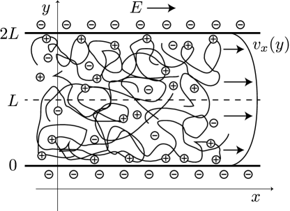
Figure 1: Schematic of the investigated system. A positively charged polyelectrolyte solution is confined within a negatively charged slit and an external electric field is applied along the slit walls. The long-chain polymers are interspersed with polymer counterions and anions derived from salt.

In this study, we assume that the electric field is sufficiently weak so that the flow speed is proportional to the field strength. Specifying a coefficient $\lambda_{12}(y)$, the flow profile is expressed as $v_{x}(y)=\lambda_{12}(y)E$. In other words, the solution is Newtonian and the nonlinear dependence of the flow on $E$ can be ignored. Having obtained the static profiles (which are difficult to solve analytically), $\lambda_{12}$ is calculated as

$$\lambda_{12}(y)=\frac{\varepsilon}{4\pi}\int^{y}_{0}\frac{dy^{\prime}}{\eta(\phi(y^{\prime}))}\left.\frac{\partial\psi}{\partial y}\right|_{y^{\prime}}.$$ (14)

This quantity is related to the macroscopic electro-osmotic coefficient in Eq. (1) by

$$L_{12}=\frac{1}{L}\int^{L}_{0}\lambda_{12}(y)dy.$$ (15)

IV Results and Discussion

To study the effects of the near-surface polyelectrolyte structures on electro-osmosis in this system, we numerically evaluate Eqs. (9), (III) and (11). The parameter settings are $c_{\mathrm{b}}=10^{-6}$Å^-3, $v=50$ų, $L=1024$Å, $\ell_{\mathrm{B}}=7$Å, $T=300$K, $\psi_{\mathrm{S}}=-k_{\mathrm{B}}T/e=-25.8$mV, $a=5$Å, and $\eta_{0}=0.01$P. Here $\ell_{\mathrm{B}}$ is the Bjerrum length, given by $\ell_{\mathrm{B}}=e^{2}/(\varepsilon k_{\mathrm{B}}T)$. The polymer chains are assumed so long that $c_{\mathrm{b}}>c^{*}$, where $c^{*}$ is the overlap concentration of the polymer solution (see Appendix B).

The electro-osmotic coefficient is evaluated from the $L_{12}^{0}$ of a solution without polyelectrolytes, given by $L_{12}^{0}=-\varepsilon\psi_{\mathrm{S}}/4\pi\eta_{0}=1.82\times 10^{-4}$cm²/V$\cdot$s. The space discretization in the numerical calculations is $d=1$Å.

IV.1 Electrically neutral polymer solution with chemically repulsive surfaces

First, we assume that polymers are electrically neutral, i.e., $f=0$. In this case, the mean-field equations (9) and (III) are exactly solved as

$$\phi = \sqrt{c_{\mathrm{b}}}\tanh\left(\frac{y}{\xi}\right),$$ (16)

$$\beta e\psi = 2\ln\frac{1+\mathrm{e}^{-\kappa y}\tanh(\beta e\psi_{\mathrm{S}}/4)}{1-\mathrm{e}^{-\kappa y}\tanh(\beta e\psi_{\mathrm{S}}/4)}.$$ (17)

where $\kappa=(8\pi\ell_{\mathrm{B}}c_{\mathrm{b}}^{+})^{1/2}$ is the Debye wave number and $\xi=a/\sqrt{3vc_{\mathrm{b}}}=408$Å  is the correlation length of the polymer concentration fluctuation. $\mathrm{e}$ is Napier’s constant. Note that these analytical solutions are valid only when $\kappa^{-1}\ll L$ and $\xi\ll L$ because they are solved under the boundary conditions at $y=0$ and $L$. If $|\beta e\psi_{\mathrm{S}}|\ll 1$, Eq. (17) reduces to

$$\psi=\psi_{\mathrm{S}}\mathrm{e}^{-\kappa y},$$ (18)

using the Debye-Hückel approximation.

If the slit width is much larger than all other length scales in the system, $L_{12}$ is approximately equal to $L_{12}\approx\lambda_{12}(L)$. Therefore, we write

$$L_{12}\approx\frac{\varepsilon}{4\pi\eta_{0}}\int^{L}_{0}\frac{dy}{1+\eta_{1}\phi}\frac{\partial\psi}{\partial y}.$$ (19)

Because $\psi(y)$ is a monotonically increasing function of $y$ in Eqs. (17) and (18), the integral $\int\cdots dy$ in Eq. (19) can be replaced by $\int\cdots d\psi$, using $\mathrm{e}^{y/\xi}=\zeta^{-1/\kappa\xi}$. $L_{12}$ is then calculated as

$$\frac{L_{12}}{L_{12}^{0}}=\int^{1}_{0}\frac{\left(\zeta^{-1/\kappa\xi}+\zeta^{1/\kappa\xi}\right)d\zeta}{(h+1)\zeta^{-1/\kappa\xi}-(h-1)\zeta^{1/\kappa\xi}},$$

(20)

where $\zeta=\psi/\psi_{\mathrm{S}}$ is a reduced electrostatic potential. After some calculations, Eq. (20) can be expanded as

$$\frac{L_{12}}{L_{12}^{0}}=\frac{2}{h+1}\frac{\kappa\xi+1}{\kappa\xi+2}+\frac{1}{h+1}\sum_{n=1}^{\infty}\left(\frac{h-1}{h+1}\right)^{n}$$

$$\times\left[\frac{1}{2n/(\kappa\xi)+1}+\frac{1}{2(n+1)/(\kappa\xi)+1}\right].$$ (21)

When $h=1$, Eq. (21) reduces to

$$L_{12}=L_{12}^{0}\left(\frac{\kappa\xi+1}{\kappa\xi+2}\right).$$ (22)

Clearly, Eq. (22) is an increasing function of $\kappa\xi$.

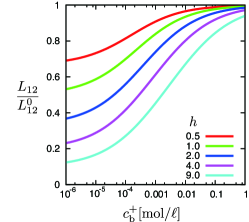
Figure 2: Electro-osmotic coefficients $L_{12}$ in the solution without polyelectrolytes, plotted as functions of salt concentration $c_{\mathrm{b}}^{+}$. In place of polyelectrolytes, electrically neutral polymers are dissolved. The viscosity parameter $h$ is varied.

The electro-osmotic coefficient calculated by Eq. (21) is plotted as a function of salt concentration in Fig. 2. Shown are the coefficients for several values of the bulk viscosity parameter $h$. As the salt concentration increases, the electro-osmotic coefficient increases and approaches $L_{12}^{0}$, regardless of $h$. By contrast, in the low salt concentration regime, $L_{12}$ decreases as $(c_{\mathrm{b}}^{+})^{1/2}$ to $L_{\rm 12}^{\mathrm{b}}=L_{12}^{0}/(1+h)$, the electro-osmotic coefficient estimated at the viscosity of the bulk solution.

We interpret these results as follows. In the neutral polymer solution, the electrostatic interaction does not influence the polymer concentration profile. The polymers are depleted from the surface by short-ranged surface forces, and the near-surface viscosity is smaller than that in the bulk. Only the region near the surface, where $\rho\neq 0$, responds to the applied electric field. The charged region is characterized by the Debye length $\kappa^{-1}$ from the surface. If the Debye length is smaller than the correlation length $\xi$, the electro-osmosis is enhanced; otherwise it is suppressed.

Given the effective viscosity $\eta_{\rm S}$, the electro-osmotic coefficient is calculated by the usual Smoluchowski’s formula, $L_{12}=-\varepsilon\psi_{\mathrm{S}}/4\pi\eta_{\mathrm{S}}$. As noted above, the formation of the depletion layer near the surface effectively lowers the viscosity of the solution. From Eq. (21), the effective viscosity decreases with $\kappa\xi$ as

$$\eta_{\mathrm{S}}\approx\eta_{0}(1+h)\left\{1-\kappa\xi\frac{h}{h-1}\ln\frac{h+1}{2}\right\},$$

(23)

when $\kappa\xi\ll 1$, using $\sum_{n=1}^{\infty}n^{-1}r^{n}=\ln[1/(1-r)]$. On the other hand, when $\kappa\xi\gg 1$, the viscosity approaches the solvent viscosity, $\eta_{\mathrm{S}}\approx\eta_{0}$. This phenomenon can be explained as follows. In the high salt limit, the electrostatic interaction between ions and walls is screened by a short length scale. If the wall is chemically repulsive to the polymers, the polymers are depleted from the surface with a correlation length far exceeding the Debye screening length.

IV.2 Polyelectrolyte solution with electrically attractive and chemically repulsive surfaces

Next, we consider polyelectrolyte solutions, i.e., $f\neq 0$. Figure 3(a) shows the electro-osmotic coefficients as functions of salt concentration. Here we fix $h=9$ and vary the fraction of charged monomers $f$. We find that, as in neutral polymer solutions (see Fig. 2), electro-osmosis is suppressed in the low salt regime. At high salt concentrations, the electro-osmotic coefficient approaches $L_{12}^{0}$. Figure 3(a) also indicates that, with increasing electric charge on the polyelectrolytes, electro-osmosis becomes more suppressed and salinity exerts a more drastic effect. In Fig. 3(b), these plots are magnified around $L_{12}=0$. Interestingly, the electro-osmotic coefficient can become negative at sufficiently dilute salt and when the polyelectrolytes are highly charged. Such inversion of electro-osmotic flow is never observed in neutral polymer solutions.

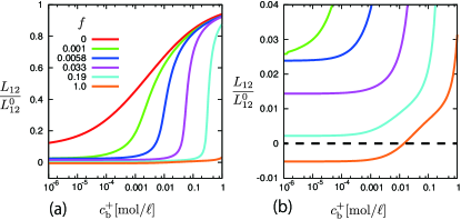
Figure 3: (a) Electro-osmotic coefficients $L_{12}$, plotted as functions of salt concentration $c^{+}_{\mathrm{b}}$. The fraction of charged monomers in the polyelectrolyte $f$ is varied for fixed $h=9$. At $f=0$, the curve is that of the electrically neutral polymer solution, and it increases with $c^{+}_{\mathrm{b}}$ as shown in Fig. 2. At sufficient salt concentrations, all curves approach $L^{0}_{12}$. (b) Magnification of the same plots around a small range of $L_{12}$.

The electo-osmotic coefficients are plotted as functions of $f$ in Fig. 4(a). Here the salt concentration is fixed at a low concentration $c_{\mathrm{b}}^{+}=10^{-6}$[mol/$\ell$], and the bulk viscosity parameter $h$ is changed. We observe that the electro-osmotic flow is weakened if the polyelectrolytes are highly charged. The mechanism of this phenomenon will be discussed later. Figure 4(a) also shows that electro-osmosis inversion occurs only at sufficiently high $h$. Figure 4(b) plots the electro-osmotic coefficient versus $h$ for $c_{\mathrm{b}}^{+}=10^{-6}$[mol/$\ell$] and $f=1$. As discussed above, the electro-osmotic flow in neutral polymer solutions saturates at $L_{12}^{\rm b}$ in the low salinity limit, according to Eq. (23). However, this equation cannot explain the curve in Fig. 4(b).

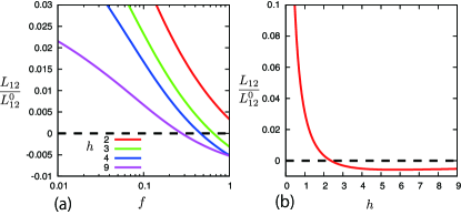
Figure 4: (a) Electro-osmotic coefficients $L_{12}$, plotted as functions of the fraction of charged monomers in the polyelectrolytes $f$. $h$ is varied at fixed salt concentration $c_{\mathrm{b}}^{+}=10^{-6}$mol/$\ell$. (b) Electro-osmotic coefficient $L_{12}$ plotted as a function of $h$. We set $c_{\mathrm{b}}^{+}=10^{-6}$mol/$\ell$ and $f=1$.

IV.2.1 Relationship between electro-osmosis and static properties

Figure. 5(a) plots the curves of $L_{12}=0$ and $L_{12}=L_{12}^{\mathrm{b}}$ in a $c_{\mathrm{b}}^{+}$-$f$ plane. As the bulk viscosity parameter $h$ decreases, the region of inverted electro-osmosis ($L_{12}<0$) shrinks and eventually disappears as $h$ becomes small. On the other hand, the $L_{12}=L_{12}^{\mathrm{b}}$ curves are less sensitive to changes in $h$. This implies that $L_{12}$ around $L_{12}^{\mathrm{b}}$ depends more on the static than kinetic properties.

To characterize the static properties, we define a quantity $\Gamma$ as

$$\Gamma=\int^{L}_{0}dy(c-c_{\mathrm{b}}).$$ (24)

$\Gamma$ measures the amount of excess adsorption of the polyelectrolytes. Figure 5(b) plots the contour lines of $\Gamma$ in the $c_{\mathrm{b}}^{+}$-$f$ plane. The $\Gamma=0$ contour characterizes the adsorption-depletion transition.Shafir_Andelman_Netz_2003 In the system investigated here, the positively charged polymers are dissolved in the slit between the negatively charged walls. Electrostatic interaction adheres the polymers to the oppositely charged wall surface. On the other hand, intermolecular interaction prevents the polymers from directly contacting the surface (see Fig. 6(a)). When the electrostatic interaction is well screened by high salt content, chemical interaction depletes the polymers from the surface vicinity.

Interestingly, when $c_{\mathrm{b}}^{+}$ is fixed, excess adsorption does not continuously increase toward $f=1$ but instead peaks at an intermediate $f$. As shown in Fig.  5(b), the polyelectrolytes with $c_{\mathrm{b}}^{+}=10^{-6}$mol/$\ell$ are most strongly adsorbed when $f\approx 5\times 10^{-3}$. This nonmonotonic behavior is counterintuitive because one expects that highly charged polyelectrolytes will be adsorbed with greatest strength. The adsorption-depletion transition has been intensively studied by Shafir et al.Shafir_Andelman_Netz_2003 Comparing Fig. 5(a) and (b), we find that the curves $L_{12}=L_{12}^{\mathrm{b}}$ roughly coincide with that of $\Gamma=0$. When the polymers are adsorbed to the surface ($\Gamma>0$), the electro-osmotic coefficient is smaller than that determined by the surface potential and bulk viscosity $L_{12}^{\mathrm{b}}$, and vice versa.

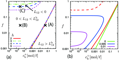
Figure 5: (a) State diagram of the electro-osmotic flow in the $c^{+}_{\mathrm{b}}$-$f$ plane. Because the polyelectrolyte concentration varies in the slit, the local viscosity depends on the distance from the wall. $L^{\mathrm{b}}_{12}$ is the electro-osmotic coefficient, estimated from the shear viscosity of the bulk solution. (b) Contours of the amount of excess adsorption, $\Gamma$, for $\Gamma=0,\;0.005$ and $0.01$. Shown are the contour lines of $L_{12}=0$ (solid) and $L_{12}=L_{12}^{\rm b}$ (broken) for $h=9$. The $\Gamma=0$ contour behaves similarly to the line $L_{12}=L_{12}^{\mathrm{b}}$ in (a).

Figure 6 shows profiles of the polymer concentration and electrostatic potential at (a) high and (b) low salt concentrations. The fraction of charged monomers is $f=0.03$. The solution conditions are as indicated in Fig. 5(a). Under low-salinity conditions, where $L_{12}<L_{12}^{\mathrm{b}}$, a peak appears in the concentration profile. Hereafter, the height and the position of the peak are denoted as $\phi_{\rm M}$ and $y_{\phi}$, respectively. As shown in Fig. 5(b), the amount of adsorption is positive (i.e., in excess) Hence, we refer to the region of $\phi>\phi_{\mathrm{b}}(=\sqrt{c_{\rm b}})$ as an adsorption layer, although the polymers themselves do not contact the surface. The electrostatic potential also peaks at $y=y_{\rm\psi}$. We call this peak an overcharging potential and its height is denoted as $\psi_{\mathrm{M}}$. We should note that the $\phi$ and $\psi$ peaks appear at different positions, with $y_{\psi}>y_{\phi}$. We also define $y_{0}$, which satisfies $\psi(y_{0})=0$. As discussed below, the adsorption layer and the overcharging potential play essential roles in the decrease and inversion of the electro-osmotic coefficient. Conversely, under high-salinity conditions, the profiles monotonically increase to the bulk values without developing peaks. The dependences of $\phi_{\rm M}$ and $\psi_{\rm M}$ on $c_{\rm b}^{+}$ and $f$ are shown in Figs. 7(a) and (b), respectively. The contours of $\phi_{\rm M}$ and $\psi_{\rm M}$ are qualitatively similar to that of $L_{12}$ in Fig. 5(a) but are dissimilar from that of the excess adsorption. This implies that the maximum amount of adsorption is not important in the electro-osmotic phenomena.

The uncolored region, in which the profile does not peak, almost coincides with that of $L_{12}>L_{12}^{\rm b}$. The gradient of the electro-osmotic flow is localized to the range of the Debye screening length from the surface (see Fig. 8(a)). Therefore, the formation of the depletion layer effectively reduces the solvent viscosity. Because the electro-osmotic flow is inversely proportional to the viscosity, depletion enhances the electro-osmosis. At the adsorption-depletion transition, the increase in $L_{12}$ caused by the depletion cancels the decrease caused by adsorption. Then, the $\Gamma=0$ curve is roughly consistent with that of $L_{12}=L_{12}^{\rm b}$. Because neutral polymers in solution do not adhere to the surface, electro-osmosis is more strongly suppressed in polyelectrolyte solutions than in neutral polymer solutions.

The uncolored region in Fig. 7(b), where $\psi_{\rm M}$ develops no peak, is slightly wider than in Fig. 7(a), where $\phi_{\rm M}$ develops no peak. This difference is delicate because the Debye screening length becomes comparable to the system size when $c_{\rm b}^{+}$ and $f$ are very small.

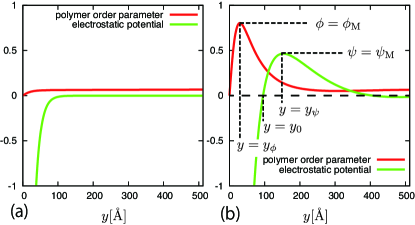
Figure 6: Profiles of the polymer order parameter $\phi$ and the electrostatic potential $\psi$ near the surface. The bulk concentrations of the salt are (a) $c_{\mathrm{b}}^{+}=0.0476$[mol/$\ell$] and (b) $c_{\mathrm{b}}^{+}=2.91\times 10^{-5}$[mol/$\ell$]. In both cases, the fraction of charged monomer in the polyelectrolyte is $f=0.03$. The profiles in (a) and (b) correspond to conditions (A) and (B) in Fig. 5(a). For a clearer representation, we plot $\phi(y)/15\phi_{\mathrm{b}}$ and $15\psi(y)/|\psi_{\mathrm{S}}|$ rather than $\phi(y)$ and $\psi(y)$.

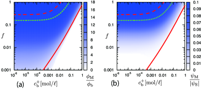
Figure 7: Effect of $c_{\rm b}^{+}$ and $f$ on the peak heights of (a) concentration profile $\phi_{\rm M}$ and (b) electrostatic potential $\psi_{\rm M}$. Shown are the contour lines of $L_{12}=0$ (broken) and $L_{12}=L_{12}^{\rm b}$ (solid) for $h=9$. The dotted line is $L_{12}=0$ estimated by Eq. (30). Uncolored regions indicate where no peaks appear in $\phi$ and $\psi$ (i.e., where $\phi_{\mathrm{M}}$ and $\psi_{\mathrm{M}}$ are undefined).

IV.2.2 Relationship between electro-osmosis and dynamical properties

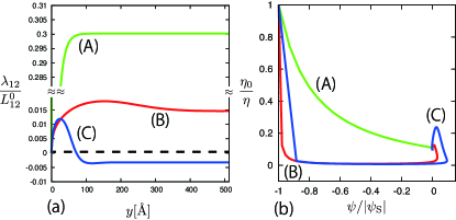
Figure 8: (a) Profiles of the electro-osmotic flow $\lambda_{12}$ in three states; (A) depletion state: $c_{\mathrm{b}}^{+}=0.0476$mol/$\ell$ and $f=0.03$. (B) adsorption state: $c_{\mathrm{b}}^{+}=2.91\times 10^{-5}$mol/$\ell$ and $f=0.03$. (C) flow inversion state: $c_{\mathrm{b}}^{+}=2.91\times 10^{-5}$mol/$\ell$, and $f=0.46$. These conditions are marked in Fig. 5(a). In condition (C), the overcharging potential is $\psi_{\mathrm{M}}/|\psi_{\mathrm{S}}|\approx 0.1$. (b) Parametric representations of $\psi(y)$ and $1/\eta(\phi(y))$ for the three states. Points $(\psi/|\psi_{\rm S}|,\eta_{0}/\eta)=(-1,1)$ and $(\psi/|\psi_{\rm S}|,\eta_{0}/\eta)=(0,1/(1+h))$ correspond to the surface ($y=0$) and bulk ($y=L$), respectively. The bulk viscosity parameter is fixed at $h=9$.

As shown in Fig. 7, $\phi_{\rm M}$ and $\psi_{\rm M}$ are large in the regime of large $f$ and small $c_{\rm b}^{+}$, where the electro-osmotic coefficient becomes negative. We emphasize that these large values of $\phi_{\rm M}$ and $\psi_{\rm M}$ are essentially important for the sign reversal of $L_{12}$.

Figure 8(a) shows the profiles of the flow field near the surface under three conditions. Here we note that $v_{x}(y)=\lambda_{12}(y)E$. Conditions (A) and (B) correspond to the adsorption and depletion states, respectively. The global electro-osmotic coefficient $L_{12}$ becomes negative under Condition (C). These conditions are marked in Fig. 5(a). In all cases, the gradient of the flow field is localized to the vicinity of the surface; that is, the flow macroscopically behaves as a plug flow. While curve (A) varies almost monotonically with $y$, curve (B) is nonmonotonic, and curve (C) is more complex. Under condition (C), the flow direction is positive near the surface, but changes at some distance from the wall, saturating at a negative value. The saturation value gives the macroscopic electro-osmotic coefficient from Eq. (15). By contrast, curve (B) remains positive across the range. If the viscosity is homogenous and independent of the polymer concentration, the flow field is easily calculated from Eq. (14) as

$$\lambda_{12}(y)=\frac{\varepsilon}{4\pi\eta}\left\{\psi(y)-\psi_{\mathrm{S}}\right\}.$$ (25)

The overcharging potential is necessary the nonmonotonic variations in (B) and (C). However, because $\psi_{\rm S}<\psi(y)$ everywhere, the overcharging potential alone cannot explain the negative $L_{12}$ given that $\eta$ is constant.

If the electrostatic potential monotonically changes with $y$ as in condition (A), $\psi=\psi(y)$ is uniquely expressed by its inverse function $y=y(\psi)$. Then, Eq. (14) is given by

$$\lambda_{12}(L)=\frac{\varepsilon}{4\pi}\int^{0}_{\psi_{\mathrm{S}}}\eta(\psi^{\prime})^{-1}d\psi^{\prime},$$ (26)

where $\eta(\psi)=\eta(\phi(y(\psi)))$ is also a unique function of $\psi$. The curves of $\eta(\psi)$ are plotted in Fig. 8(b). Since $\eta(\psi)$ is positive, $\lambda_{12}(L)$ is also positive, indicating that the flow toward $E$ is maintained.

When the overcharging potential arises, as in conditions (B) and (C), $y$ is a multivalued function of $\psi$, which invalidates Eq. (26). In this case, Eq. (14) becomes

$$\frac{4\pi}{\varepsilon}\lambda_{12}(L) = \int_{0}^{y_{\psi}}\frac{dy^{\prime}}{\eta(y^{\prime})}\left.\frac{\partial\psi}{\partial y}\right|_{y^{\prime}}+\int_{y_{\psi}}^{L}\frac{dy^{\prime}}{\eta(y^{\prime})}\left.\frac{\partial\psi}{\partial y}\right|_{y^{\prime}}$$ (27)

$$= \int^{\psi_{\mathrm{M}}}_{\psi_{\mathrm{S}}|y<y_{\psi}}\frac{d\psi^{\prime}}{\eta(\psi^{\prime})}-\int^{\psi_{\mathrm{M}}}_{0|y>y_{\psi}}\frac{d\psi^{\prime}}{\eta(\psi^{\prime})}.$$

Here we should note that the paths of the two integrals in Eq. (27) differ from each other.

According to linear analysis, the electrostatic potential profile may have multiple peaks.Chatellier_Joanny_1996 The intensities of the peaks decay with increasing distance from the wall. We assume that the highest peak (nearest the wall) plays a dominant role in the electrokinetic flow and ignore the contributions of the remaining peaks.

Figure 9 is a schematic of Eq. (27). When the electrostatic potential overcharges, the curve of $1/\eta(\psi)$ is divisible into three segments. These segments delineate three realms, with areas denoted by $S_{1}$, $S_{2}$, and $S_{3}$. Within the slit, the realms correspond to the ranges $S_{1}$: $0<y<y_{0}$, $S_{2}$: $y_{0}<y<y_{\psi}$, and $S_{3}$: $y_{\psi}<y<L$ (see Fig. 6(b)). The first and second terms in Eq. (27) are given by $S_{1}+S_{2}$ and $S_{2}+S_{3}$, respectively. In terms of these areas, the electro-osmotic coefficient is given by $L_{12}=(S_{1}+S_{2})-(S_{2}+S_{3})=S_{1}-S_{3}$. If $S_{1}<S_{3}$, the macroscopic flow is inverted.

Using Eq. (27), we devise a simple method for estimating the electro-osmotic coefficient in adsorption states. The viscosity is assumed constant within each realm. More precisely, we assume that polymer concentration is fixed at $\phi=\phi_{\rm M}$ within the range $0<y<y_{\rm\psi}$ and at $\phi=\phi_{\rm b}$ in $y_{\rm\psi}<y<L$. These approximations are schematically represented in Fig. 9(b). $S_{1}$ and $S_{3}$ are then approximated as

$$S_{1} \approx \frac{\varepsilon}{4\pi}\frac{-\psi_{\rm S}}{\eta_{\rm S}},$$ (28)

$$S_{3} \approx \frac{\varepsilon}{4\pi}\left(\frac{1}{\eta_{\rm b}}-\frac{1}{\eta_{\rm S}}\right)\psi_{\rm M},$$ (29)

where $\eta_{\rm S}=\eta_{0}(1+h\phi_{\rm M}/\phi_{\rm b})$ and $\eta_{\rm b}=\eta_{0}(1+h)$. Finally, we obtain

$$L_{12}\approx\frac{\eta_{\rm b}}{\eta_{\rm S}}L_{12}^{\rm b}+\left(1-\frac{\eta_{\rm b}}{\eta_{\rm S}}\right)L_{12}^{\rm M},$$ (30)

where $L_{12}^{\rm M}=-\varepsilon\psi_{\rm M}/(4\pi\eta_{\rm b})$ is the electro-osmotic coefficient estimated by the overcharging potential. The $L_{12}=0$ curve estimated by Eq. (30) is drawn in Fig. 7. This curve is qualitatively consistent with the numerical solutions. In this estimation, the overcharging potential does not directly cause the inversion of electro-osmotic flow; formation of the highly viscous layer is also important.

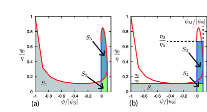
Figure 9: (a) Schematic for calculating $L_{12}$ in adsorption states from Eq. (27). $\psi$ and $1/\eta$ are parameterized with respect to $y$. (b) Approximate representation of $\psi$-$\eta^{-1}$ in (a). This approximation gives a simple form of $L_{12}$, Eq. (30).

V Summary and Remarks

Applying a continuum model, we study electro-osmosis in polymer solutions. From numerical calculations and theoretical estimations, we elucidated the behaviors of the electro-osmosis in polymer solutions. The dependence of viscosity on the polymer concentration plays an important role in our model. Our main results are summarized below.

• Even if the polymer solution sandwiched between chemically repulsive walls is electrically neutral, electro-osmosis depends on the salt concentration. Decreasing the salinity suppresses the electro-osmosis.

• In polyelectrolyte solutions, the formed adsorption layer effectively enlarges the viscosity in the vicinity of the surfaces. Consequently, electro-osmosis is suppressed much more strongly in polyelectrolyte than in neutral polymer solutions. If a sufficiently high proportion of the monomers are charged and if the salt concentration is sufficiently low, the electro-osmotic flow can be inverted.

• We propose a simple equation for estimating the electro-osmotic coefficient in adsorption states (Eq. (30)). This equation captures the essential features of the inversion of the electro-osmotic coefficient, shown in Fig. 7. According to this expression, inversion is caused by two factors; enhancement of the viscosity by the near-surface adsorption layer and overshoot of the electrostatic potential.

We conclude this paper with the following remarks.

• Charge inversion and mobility reversal induced by multivalent electrolytes has been frequently reported.Grosberg_Nguyen_Shklovskii_2002 Grosberg et al.Grosberg_Nguyen_Shklovskii_2002 concluded that such phenomena depend on fluctuation correlations among the multivalent ions, which are excluded in usual Poisson-Boltzmann approaches. Our mean-field approach predicts that similar inversion phenomena occur in polyelectrolyte solutions. According to a molecular dynamics simulation, the phenomena occurs even in monovalent ions solutions confined within nanochannels.Qiao_Aluru_2004 The flow profiles obtained in the earlier study are quite similar to ours; near the surface, the flow is directed toward the electric field, but in the bulk, it is against the field.

• This article considers only limited situations; The surfaces are assumed to chemically and electrostatically repel the polymers. If the surfaces are chemically attractive, the adsorption is much enhanced by chemical forces.Joanny_1999 ; Shafir_Andelman_2004 The electro-osmotic properties of these surfaces are equally interesting and important.

• From the Onsager reciprocal relations, the electro-osmotic coefficient $L_{12}$ should equal $L_{21}$ in Eq. (2). The latter represents the electric current due to the mechanical pressure difference. Interestingly, the Onsager coefficient $L_{21}$ is inverted when $f$ is large and $c_{\rm b}^{+}$ is sufficiently small.

• In the above numerical and theoretical analyses, the viscosity parameter $h$ is assumed constant, although in practice it depends on the fraction of charged monomers $f$ and the salt concentration $c_{\rm b}^{+}$. When $f$ is large and $c_{\rm b}^{+}$ is small, the solution viscosity increases (see Appendix B). Our studies indicate that large $f$ and small $c_{\rm b}$ favor flow inversion. The same trends were observed for large $h$. If we set $h$ as a function of $f$ and $c_{\rm b}$, more dramatic changes would appear in the curves of $L_{12}$ against $f$ and $c_{\rm b}^{+}$. Although the $L_{12}$ and the phase diagrams would quantitatively alter, the qualitative trends, i.e., suppression of the electro-osmotic flow and inversion at large $f$ and a small $c_{\rm b}^{+}$, should remain intact.

Appendix A Local equilibrium conditions for the components

Because we apply an external field $E$ along the $x$ direction (see Fig. 1), the total electrostatic potential is not $\psi(y)$ in Eq. (6), but instead is $\Psi(x,y)=\psi(y)-Ex$. Assuming the local equilibrium condition, the chemical potential of the $i$-th species is given by

$$\mu^{i}=k_{\rm B}T\ln(c^{i}a^{3})+ez_{i}\Psi,$$ (31)

where $z_{i}$ is the charge of the $i$-th ion. In the geometry of the investigated system, the diffusion flux of the ion, given by $\mbox{\boldmath$j$}^{i}=-D^{i}c^{i}\nabla\mu^{i}$, is divided into two components:

$$\mbox{\boldmath$j$}^{i} = j^{i}_{y}\mbox{\boldmath$e$}_{y},+j^{i}_{x}\mbox{\boldmath$e$}_{x},$$ (32)

$$j^{i}_{y} = -D^{i}c^{+}\frac{\partial}{\partial y}\left[k_{\rm B}T\ln(c^{i}a^{3})+ez_{i}\psi(y)\right]$$ (33)

$$j^{i}_{x} = D^{i}z_{i}c^{i}E.$$ (34)

Here $D^{i}$ is the diffusion constant of the $i$-th ion, and $\mbox{\boldmath$e$}_{x}$ and $\mbox{\boldmath$e$}_{x}$ are the unit vectors along the $x$ and $y$ axes, respectively. Because the system is confined by the walls at $y=0$ and $2L$, the diffusion flux along the $y$ direction vanishes at steady state. Thus, we obtain the Boltzmann distribution along the $y$ axis as $c^{i}a^{3}\propto\exp\{-z_{i}e\psi/k_{\rm B}T\}$. On the other hand, the diffusion flux remains along the $x$ axis. Because the applied electric field is sufficiently weak and orthogonal to $-\nabla\psi$, it influences neither the concentration fields nor the polymer conformation.

Appendix B Scaling behaviors in polyelectrolyte solutions

The scaling behaviors of polyelectrolyte solutions are known to widely differ from those of uncharged polymer solutions. At the overlap concentration $c^{*}$ in a polyelectrolyte solution, the monomer density inside the coil equals the overall monomer density in the solution.Dobrynin_Colby_Rubinstein_1995 In our notation, the overlap concentration in a theta solvent is determined by $c^{*}(1+2c_{\rm b}^{+}/c^{*}f)^{-3/2}\approx N^{-2}a^{-2}\ell_{\rm B}^{-1}f^{-2}$.

In the low-salt or salt-free regime, the overlap concentration becomes $c^{*}\approx(a^{2}\ell_{\rm B}Nf)^{-1}$. Conversely, it approaches $c^{*}\cong\{8(c_{\rm b}^{+})^{3}a^{-4}\ell_{\rm B}^{-2}f^{-7}N^{-4}\}^{1/5}$ in the high-salt regime. Between these two extremes, the overlap concentration decreases as $f$ increases. Given the same polymer length $N$, polyelectrolyte chains expand more than their uncharged counterparts.

The viscosity of polyelectrolyte solutions also obeys scaling behaviors, which depend on the solvent quality and the polymer concentration regime. For example, the viscosity of a semidilute solution in a theta solvent is given by $\eta\approx\eta_{0}Na\ell_{\mathrm{B}}^{1/2}fc^{1/2}(1+2c_{\mathrm{b}}^{+}/fc)^{-3/4}$. If the salt is not dissolved or is insufficiently dilute, this expression approaches $\eta\approx\eta_{0}Na\ell_{\mathrm{B}}^{1/2}fc^{1/2}$; that is, the viscosity is proportional to $c^{1/2}$ (Fuoss law). On the other hand, in highly saline conditions the viscosity behaves as $\eta\approx\eta_{0}Na\ell_{\mathrm{B}}^{1/2}(c_{\mathrm{b}}^{+})^{-3/4}f^{7/4}c^{5/4}$. The viscosity depends on the polymer concentration as $c^{5/4}$, identical to that of an uncharged polymer solution in a theta solvent, namely $\eta\approx\eta_{0}N(ca^{3})^{1/(3\nu-1)}$ with $\nu=3/5$. Physically, this result implies that electrostatic interactions in a polyelectrolyte solution are well screened by the salt.

References

- (1) M. Rubinstein and G. A. Papoian, Soft Matter 8, 9265 (2012); and references therein.
- (2) F. Oosawa, Polyelectrolytes, Marcel Dekker, Inc. (1971).
- (3) P. G. de Gennes, Scaling Concepts in Polymer Physics, Cornell University Press (1979).
- (4) J.F. Joanny and L. Leibler, J. Phys. (France) 51, 545 (1990).
- (5) J.L. Barrat and J.F. Joanny, Advances in Chemical Physics XCIV, 1 (1996).
- (6) A. V. Dobrynin and M. Rubinstein, Prog. Polym. Sci. 30, 1049 (2005).
- (7) T. Igarashi et al., Kobunshi Ronbunshu 48, 751 (1991).
- (8) M. Liu and J. Yang, Microvascular Res. 78, 14 (2009).
- (9) R. W. O’Brien and L. R. White, J. Chem. Soc. Faraday Trans. II 74, 1607 (1978).
- (10) D. Burgreen and F. R. Nakache, J. Phys. Chem. 68, 1084 (1964).
- (11) C. L. Rice and R. Whitehead, J. Phys. Chem. 69, 4017 (1965).
- (12) B. S. Levine, J. R. Marriott, K. Robinson, J. Chem. Soc. Faraday Trans. II 71, 1 (1974).
- (13) J.F. Joanny, L. Leibler, P. G. de Gennes, J. Polym. Sci. Poym. Phys. Ed. 17, 1073 (1979).
- (14) P. G. de Gennes, Macromolecules 14, 1637 (1981).
- (15) P. G. de Gennes, Macromolecules 15, 492 (1982).
- (16) I. Borukhov, D. Andelman, H. Orland, Eurphys. Lett. 32, 499 (1995).
- (17) X. Châtellier and J.F. Joanny, J. Phys. II France 6 1669 (1996).
- (18) I. Borukhov, D. Andelman, H. Orland, Macromolecules 31, 1665 (1998).
- (19) J.F. Joanny, Eur. Phys. J. B 9, 117 (1999).
- (20) A. Shafir, D. Andelman, R. R. Netz, J. Chem. Phys. 119, 2355 (2003).
- (21) A. Shafir and D. Andelman, Phys. Rev. E 70, 061804 (2004).
- (22) H. Vink, J. Chem. Soc., Faraday Trans. I 84, 133 (1988).
- (23) M. S. Bello et al., Electrophoresis 15, 623 (1994).
- (24) M. Otevřel and K. Klepárník, Electrophoresis 23, 3574 (2002).
- (25) C. Zhao, E. Zholkovskij, J. H. Masliyah, C. Yang, J. Colloid Interface Sci. 326, 503 (2008).
- (26) M. L. Olivares, L. Vera-Candioti, C. L. A. Berli, Electrophoresis 30, 921 (2009).
- (27) C. Zhao and C. Yang, J. Non-Newtonian Fluid Mech. 166, 1076 (2011).
- (28) A. V. Dobrynin, R. H. Colby, M. Rubinstein, Macromolecules 28, 1859 (1995).
- (29) A. Yu. Grosberg, T. T. Nguyen, B. I. Shklovskii, Rev. Mod. Phys. 74, 329 (2002).
- (30) R. Qiao, N. R. Aluru, Phys. Rev. Lett. 92, 198301 (2004).