Hole Spin Helix: Anomalous Spin Diffusion in Anisotropic Strained Hole Quantum Wells

Abstract

We obtain the spin-orbit interaction and spin-charge coupled transport equations of a two-dimensional heavy hole gas under the influence of strain and anisotropy. We show that a simple two-band Hamiltonian can be used to describe the holes. In addition to the well-known cubic hole spin-orbit interaction, anisotropy causes a Dresselhaus-like term, and strain causes a Rashba term. We discover that strain can cause a shifting symmetry of the Fermi surfaces for spin up and down holes. We predict an enhanced spin lifetime associated with a spin helix standing wave similar to the Persistent Spin Helix which exists in the two-dimensional electron gas with equal Rashba and Dresselhaus spin-orbit interactions. These results may be useful both for spin-based experimental determination of the Luttinger parameters of the valence band Hamiltonian and for creating long-lived spin excitations.

Systems with spin-orbit interactions have generated great academic and practical interest S. A. Wolf et. al. (2001); Murakami et al. (2003); C.L. Kane and E.J. Mele (2005); B.A. Bernevig and S.C. Zhang (2006); Wenk et al. (2010) because they allow for purely electric manipulation of the electron spin Nitta et al. (1997); Grundler (2000); Y. Kato et. al. (2004), which could be of use in areas ranging from spintronics to quantum computing. However spin-orbit interactions have also the undesired effect of causing spin decoherence M. I. Dyakonov et. al. (1986). Recently a new mechanism by which a system can sustain both strong spin-orbit interactions and long spin relaxation times has been proposed B.A. Bernevig et al. (2006). In properly tuned systems a non-decaying spin density standing wave can be excited. This Persistent Spin Helix (PSH) has been observed through spin transient experiments in electron doped GaAs quantum wells. C.P. Weber and J. Orenstein et. al (2007); J. Koralek et al. (2009)

In electron doped samples the PSH occurs when the Rashba and Dresselhaus spin-orbit interaction strengths are tuned to match each other. At equal strength the spin dynamics conserve an $SU(2)$ triplet of spin operators, two of which describe spin standing waves, while the third describes a uniform spin density that is selected and preserved by the tuned spin-orbit interaction. The triplet’s infinite lifetime is obtained by tuning the spin-orbit interaction to have a constant phase independent of electron momentum, in which case the electron spin structure is independent of momentum and conserved under scattering. In particular, the Rashba and linear Dresselhaus terms are proportional to $k_{-}=k_{x}-\imath k_{y}$ and to $k_{+}=k_{x}+\imath k_{y}$ respectively, so when they are at equal strength the total spin-orbit interaction has constant phase, producing long-lived spin excitations.

The experimental discovery of the PSH in the 2-D electron gas raises the question of whether it exists in other systems. Recently one of us predicted that tuned topological insulators can host PSHs with very long lifetimes Sacksteder et al. (2012). Here we examine 2-D hole gases under strain, calculate the spin orbit interaction of the heavy holes, and find Rashba and Dresselhaus-like terms caused respectively by applied strain and anisotropy. When fine-tuned properly the spin orbit term has constant phase, producing long-lived spin helices aligned with the strain axis and an anomalous enhancement of the spin lifetime. These results apply also to other systems which like holes are four-fold degenerate at the $\Gamma$ point, such as the metallic phase predicted in pyrochlore iridates. Yang and Kim (2010); Wan et al. (2011); Witczak-Krempa and Kim (2012) PSHs are a general phenomenon that can be realized in diverse systems with a wide variety of tuning parameters.

Hole-doped quantum wells are sensitive to applied strain and to anisotropy, which are key to the spin physics uncovered here. Unlike the electron gas, in the 2-D hole gas the spin components $S_{x},S_{y},S_{z}$ are decoupled at leading order if there is neither strain nor anisotropy T.L. Hughes et al. (2006). This is due to the holes’ spin-orbit interaction $H_{\text{SO}}$, which determines the couplings between spin components. In the unstrained isotropic hole gas this operator has a cubic form with f-wave symmetry $H_{\text{SO}}=\alpha(k_{+}^{3}\sigma_{-}-k_{-}^{3}\sigma_{+})$ and hence vanishes when integrated over the isotropic Fermi surface. However recent experiments performed by attaching a piezo to hole-doped GaAs samples have revealed that strain can be used to cause large changes in the spin orbit interaction Kolokolov et al. (1999); Kraak et al. (2004); Habib et al. (2007); J. Shabani et al. (2008). The experimental results largely confirm the standard Kane and Luttinger $\vec{k}\cdot\vec{p}$ Hamiltonian which predicts that strain and anisotropy substantially deform the two heavy hole Fermi surfaces Winkler (2000); Kolokolov et al. (1999); Kraak et al. (2004); J. Shabani et al. (2008). For a certain critical value of the strain field, the surfaces meet at two special ”touching points”, which causes an experimentally confirmed Kraak et al. (2004) magnetic breakdown of Shubnikov-de Haas (SdH) orbits. These touching points hint at interesting spin dynamics, because similar degeneracies are seen in the Fermi surfaces of electron-doped systems when they are tuned to produce PSHs.

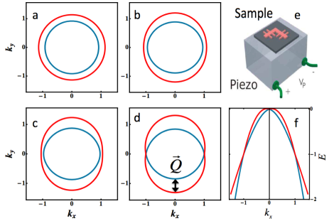
Figure 1: Tuning the strain produces touching points in the heavy hole Fermi surfaces, which are shown at zero strain $\beta^{2}=0$ (pane a) and intermediate strains (b) $0.4\cdot k_{F}^{2}$ and (c) $0.6\cdot k_{F}^{2}$. Finally pane (d) and (f) show critical strain $\beta^{2}=k_{F}^{2}$, with two touching points on the $k_{x}$ axis. At critical strain shifting by $\pm\vec{Q}$ places one band on top of the other, as seen in pane (d). The strain is oriented along the $x$ axis, and $\gamma_{2}/\gamma_{3}=1$. Identical results are obtained when the sign of $\gamma_{2}/\gamma_{3}$ is reversed and the strain axis is rotated by 90 degrees. $E_{F}=1$ and $\alpha=0.2$. Pane (e): schematic of a sample glued on a strain-generating piezo as used in Ref. Habib et al. (2007).

Usually the heavy hole Fermi surfaces and their deformation under strain are modeled with considerable accuracy within the $4$-band Luttinger model Luttinger (1956) or the $8$-band Kane Hamiltonian Kane (1957). These models unfortunately obscure the spin-orbit interaction between the two heavy hole states and prohibit analytical calculation of the spin-charge dynamics. We will therefore focus only on the heavy holes, and will make explicit their spin-orbit interaction $H_{\text{SO}}$, which is simply the off-diagonal element of the two-band effective Hamiltonian which governs the heavy holes. Various previous works have developed two-band models of the heavy holes Kleinert and Bryksin (2007); Raichev (2008); Liu et al. (2008); Wang and Wu (2012); Dollinger et al. (2013); ours distinguishes itself by including strain.

We derive our two-band Hamiltonian from the 4-band Luttinger Hamiltonian $H_{0}$, which describes the total angular momentum $j=3/2$ band that lies nearest to the Fermi surface. There are four states: two heavy holes with $j_{z}=\pm 3/2$ and two light holes with $j_{z}=\pm 1/2$. Following common practice, we choose the bulk Hamiltonian appropriate for crystal growth along the high-symmetry $z$ (001) axis, and we take the hole carrier concentration to be small enough that only the first 2-D subband in the quantum well contributes to transport. Kamburov et al. (2012); Kolokolov et al. (1999); Kraak et al. (2004); Dai et al. (2009); Dollinger et al. (2013); Scholz et al. (2013); Ekenberg and Altarelli (1985); Liu et al. (2008); Lu et al. (2005); Winkler (2000) We include a strain field $\epsilon_{ij}$ using the Bir-Pikus strain Hamiltonian $H_{\epsilon}$ Bir and Pikus (1974), and we model the quantum well with a confinement potential $V_{c}$ and a small charge asymmetry $V_{E}=-eEz$;

$$H=H_{0}+H_{\epsilon}+V(z),\;V(z)=V_{c}+V_{E}$$ (1)

$$H_{0}=\frac{1}{2m}\left({\gamma_{1}+\frac{5}{2}\gamma_{2}}\right)|\vec{k}|^{2}-\frac{\gamma_{2}}{m}k_{i}^{2}S_{i}^{2}-2\frac{\gamma_{3}}{m}\{k_{i},k_{j}\}\{S_{i},S_{j}\}$$

$$H_{\epsilon}=a\epsilon_{ii}+b\epsilon_{ii}S_{i}^{2}+d\epsilon_{ij}\{S_{i},S_{j}\}$$

$\vec{S}$ is a spin $3/2$ matrix. The double index implies summation (in the anticommutators, do not sum over ${i=j}$), and $\{A,B\}=\frac{1}{2}(AB+BA)$. We will show that hole spin physics is a sensitive measure of anisotropy in the valence band, which is parameterized by three Luttinger parameters $\gamma_{i}$. $\gamma_{1},\gamma_{2}$ control the hole masses along the $z$ axis, while $\gamma_{1},\gamma_{3}$ control the masses along the $[111]$ axis. Both these parameters and the strain deformation potentials $a,b,$ and $d$ have widespread applications and are reported in standard reference works. Lan (1982); Vurgaftman et al. (2001)

The Luttinger Hamiltonian has the most general form possible for a $\vec{k}\cdot\vec{p}$ model with four degenerate bands (angular momentum $j=3/2$) in a crystal with both cubic discrete symmetry and time reversal symmetry. Zinc blende semiconductors are not symmetric under inversion and therefore possess only tetrahedral symmetry which is a subgroup of cubic symmetry, but this asymmetry is weak in the bulk Lipari and Baldareschi (1970). Several works have examined terms beyond the Luttinger Hamiltonian and developed their effects on heavy holes Winkler (2000, 2003); Raichev (2008); Dollinger et al. (2013). Here we retain only the Luttinger Hamiltonian and use an explicit term $V_{E}=-eEz$ to break inversion symmetry.

The spin-orbit physics can be illuminated by breaking the Hamiltonian explicitly into the heavy hole sector $j_{z}=+3/2,\,-3/2$ and the light hole sector $j_{z}=+1/2,\,-1/2$:

$$H = V(z)+\begin{bmatrix}1\cdot k_{HH}&U_{HL}\\ U_{HL}^{\dagger}&1\cdot k_{LL}\end{bmatrix},\;U_{HL}=\begin{bmatrix}S&R^{*}\\ R&-S^{*}\end{bmatrix}$$

$$S = -d(\imath\epsilon_{zy}-\epsilon_{zx})-\sqrt{3}\gamma_{3}k_{-}k_{z}/m$$ (2)

$$R = -\frac{\sqrt{3}}{4m}(k_{+}^{2}(\gamma_{2}+\gamma_{3})+k_{-}^{2}(\gamma_{2}-\gamma_{3})-2\gamma_{3}\beta^{2}e^{\imath 2\theta})$$

The in-plane strain is encapsulated in a magnitude $\beta^{2}$ and orientation $\theta$ which are set by $\beta^{2}e^{\imath 2\theta}=b\frac{m}{\gamma_{3}}(\epsilon_{xx}-\epsilon_{yy})+\imath\frac{2m}{\sqrt{3}\gamma_{3}}d\epsilon_{xy}$. The kinetic terms $k_{HH}$ and $k_{LL}$ are respectively equal to $(\gamma_{1}+\gamma_{2})k^{2}/2m+(\gamma_{1}-2\gamma_{2})k_{z}^{2}/2m$ and $(\gamma_{1}-\gamma_{2})k^{2}/2m+(\gamma_{1}+2\gamma_{2})k_{z}^{2}/2m$, plus a strain-induced constant splitting. $S$ couples holes with the same sign of $j_{z}$, while $R$ couples holes with opposite sign.

This explicit representation reveals that there is no direct interaction either between the $j_{z}=\pm 3/2$ heavy holes or between the $j_{z}=\pm 1/2$ light holes. In consequence the spin-orbit interaction between the heavy holes is proportional to $R^{*}$. This is an exact result. It informs us that when $R=0$ there is a degenerate point in the dispersion, where the two heavy hole bands meet Kolokolov et al. (1999). In fact, addition of a tuned strain field generically creates two such degenerate points on the Fermi surface. Figure 1 illustrates this in the particular case of compression along the $x$ axis. In this special case the two degenerate points lie on the same axis and occur when the strain is tuned for resonance with the Fermi momentum $\beta=k_{F}$.

We procede by deriving the exact two-band effective Hamiltonian which controls the heavy holes, $H_{HH}=V(z)+1\cdot k_{HH}+U_{HL}G_{LL}U_{HL}^{\dagger}$, where $G_{LL}=(E-k_{LL}-V(z))^{-1}$ is the light hole Green’s function. (See the supplementary material for an expanded derivation.) This can be rewritten as

$$H_{HH} = \left(\begin{array}[]{cc}\hat{k}_{HH}&H_{\text{SO}}\\ H_{\text{SO}}^{*}&\hat{k}_{HH}\\ \end{array}\right),\;H_{\text{SO}}=-[G_{LL},S]R^{*}$$ (5)

$$\hat{k}_{HH} = k_{HH}+V(z)+SG_{LL}S^{*}+RG_{LL}R^{*}$$ (6)

The commutator $[G_{LL},S]=-\sqrt{3}\gamma_{3}k_{-}/m[G_{LL},k_{z}]$ is insensitive to strain and its phase is set by $\imath k_{-}$. Therefore the phase of the spin-orbit interaction is determined by $\imath k_{-}R^{*}$. We make this exact result explicit by writing the spin-orbit interaction as $H_{\text{SO}}=-\imath\alpha\frac{2m}{\sqrt{3}\gamma_{3}}k_{-}R^{*}={\imath\alpha}(k_{-}^{3}(1+\gamma_{2}/\gamma_{3})/2-k^{2}k_{+}(1-\gamma_{2}/\gamma_{3})/2-k_{-}\beta^{2}e^{-\imath 2\theta})$. The spin-orbit strength $\alpha=-\imath 3\gamma_{3}^{2}/2m^{2}[G_{LL},k_{z}]$ is determined by the quantum well’s confinement potential $V_{c}$. It can be approximated analytically in a thin well with thickness $L$, where confinement creates a splitting $\Delta E\sim 2\frac{\gamma_{2}}{m}\langle k_{z}^{2}\rangle\propto 2\frac{\gamma_{2}}{m}(2\pi/L)^{2}$ between the heavy and light hole bands. This energy scale justifies neglect of higher orders in the potential $V_{E}$ and in $k_{x},k_{y}$. At leading order $\alpha=6\imath[V_{E},k_{z}](\gamma_{3}/2m\Delta E)^{2}$. The $k_{z}$ appearing here is an operator and does not commute with the quantum well’s built-in electric field; $[V_{E},k_{z}]=-ieE$. Similar approximations determine that $\hat{k}_{HH}=\frac{k^{2}}{2m_{H}}$, where the renormalized mass is $m_{H}=m/(\gamma_{1}+\gamma_{2}-3\gamma_{3}^{2}/\gamma_{2})$.

The first term in $H_{\text{SO}}$ stands alone when there is neither strain nor anisotropy. It is cubic in the spin-orbit strength and has f-wave character, reproducing the cubic dominance which is well known for holes Winkler (2000). Optimal spin lifetimes are obtained only in the anisotropic limit $\gamma_{2}/\gamma_{3}=-1$ where this term is entirely absent. Anisotropy and strain produce the second and third terms, which respectively have Dresselhaus ($k_{+}$) and Rashba ($k_{-}$) character. The spin-orbit interaction $H_{SO}$ has constant phase when the strain term’s magnitude is tuned to match the magnitude of the anisotropy term, i.e. when $\beta=k_{F}\sqrt{(1-\gamma_{2}/\gamma_{3})/2}$. A truly constant phase is not achievable because $H_{SO}$ induces small anisotropies in the Fermi surface which are of order $E_{SO}/E_{F},\;E_{SO}=\alpha k_{F}^{3}$. However when the strain is tuned properly these phase fluctuations are very small, one component of the spin almost commutes with the Hamiltonian, and its lifetime becomes very large.

Strain can also tune the Fermi surfaces of the spin $\uparrow$ and $\downarrow$ heavy holes to produce a quasi shifting symmetry (Eq. 7) that is key to persistent spin helices, which together with the quasi-conserved spin form a long-lived $SU(2)$ spin triplet. PSHs occur when the spin $\uparrow$ and $\downarrow$ Fermi surfaces, $\epsilon_{\uparrow,\downarrow}$, have identical shapes so that a shift of $\vec{q}=\pm\hat{Q}$ moves one Fermi surface on top of the other. This shifting symmetry can be written as:

$$\epsilon_{\downarrow}(\vec{k})=\epsilon_{\uparrow}(\vec{k}+\vec{Q}).$$ (7)

Using our heavy hole Hamiltonian, Figure 1d shows that when the Fermi surfaces are tuned for degeneracy ($\beta=k_{F}$) they also obey the shifting symmetry that produces PSHs. This is true both in the isotropic limit $\gamma_{2}/\gamma_{3}=+1$ and in the strongly anisotropic limit $\gamma_{2}/\gamma_{3}=-1$. In both limits the energy dispersion simplifies to $E_{\pm}=(\vec{k}\pm\vec{Q}/2)^{2}/2m$ on the circle defined by $|\vec{k}|=k_{F}=\beta$. Therefore at leading order in the spin-orbit strength $E_{SO}/E_{F}$ the Fermi surfaces are circles offset from each other by $\pm\vec{Q}$, and produce a spin helix standing wave. The helix’s wave-vector has magnitude $|\vec{Q}|=2k_{F}E_{\text{SO}}/E_{F}$, is proportional to the spin-orbit strength, and is independent of scattering.

The magnetoresistance is very sensitive to this physics. When the spin-orbit interaction has constant phase the magnetoresistance will become null or even change sign. If the Fermi surfaces do not fulfill the nesting condition required by a PSH then there will be neither weak localization nor antilocalization (null magnetoresistance). If a PSH exists then there will be a complete reversal from weak localization to weak antilocalization, from negative to positive magnetoresistance.

Figure 2: Diagram illustrating the scattering that produces spin-charge diffusion. Here two scattering events are shown. $G^{A}$ and $G^{R}$ describe time evolution of the hole $\psi$ and its complex conjugate $\psi^{\dagger}$. Each scattering event causes correlations between $G^{A}$ and $G^{R}$ and is shown as a dashed line connecting the two.

It may not be easy to observe these long spin lifetime effects, since semiconductors possess an approximate spherical symmetry Lipari and Baldareschi (1970) which places many of them near the isotropic limit $\gamma_{2}/\gamma_{3}=1$. However silicon is a notable exception, with $\gamma_{2}/\gamma_{3}=0.23$ Lan (1982). Moreover in many compounds there is considerable scatter in both experimental and theoretical estimates of $\gamma_{2}$ and $\gamma_{3}$, and certain authors have assigned GaP Vurgaftman et al. (2001) , SiC Willatzen et al. (1995), and Boron-doped diamond Willatzen et al. (1994) values of $\gamma_{2}/\gamma_{3}=0.17,0.24,$ and $-0.16$ respectively. Lastly $\gamma_{2}/\gamma_{3}$ remains completely unknown in the metallic phase of the pyrochlore iridates. In these materials measurement of spin dynamics may prove to be a sensitive means of determining $\gamma_{2}/\gamma_{3}$.

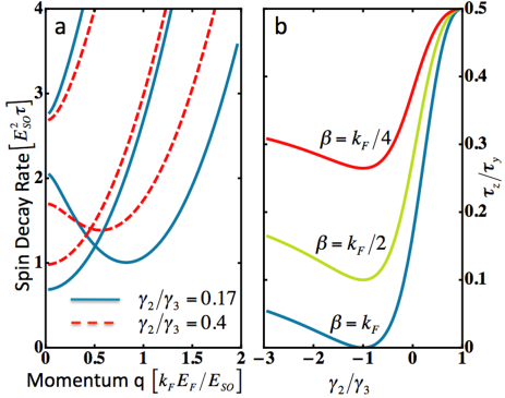
Figure 3: Strain-assisted suppression of spin decay. Pane (a) shows the spin decay’s dependence on momentum when the strain is at its optimal value $\beta=k_{F}\sqrt{(1-\gamma_{2}/\gamma_{3})/2}$. Both $\vec{q}$ and the strain are aligned with the $x$ axis. Three decay rates are shown corresponding to $S_{y}$ and to linear combinations of $S_{x}$ and $S_{z}$. $S_{y}$’s decay rate is smallest at $q=0$, while the $S_{x},S_{z}$ rates are minimized at finite momenta $\pm|\vec{Q}|=\pm(1-\gamma_{2}/\gamma_{3})k_{F}E_{F}/E_{\text{SO}}$. These long-lived $\pm|\vec{Q}|$ excitations are the persistent spin helices. The minimum decay rates of both $S_{y}$ and the PSHs go to zero when $\gamma_{2}/\gamma_{3}=-1$, signaling that neither $S_{y}$ nor the PSHs decay. Pane (b) illustrates this with the ratio $\tau_{z}/\tau_{y}$ of the decay times of spatially uniform $S_{z},S_{y}$ spin distributions. This ratio is proportional to the $S_{y}$ decay rate, and is zero at optimal $\gamma_{2}/\gamma_{3}=-1$ and optimal strain $\beta=k_{F}$.

Intrigued by this possibility, we study the equations of motion governing diffusion of the heavy holes, neglecting excitation and diffusion of light holes for analytic tractability. The heavy holes form a doublet with spin $\pm\frac{1}{2}$ and total angular momentum $j_{z}=\pm\frac{3}{2}$; we write the charge density $N$ and the spin densities $S_{i}$ as a $4-$vector $\vec{\rho}=\begin{bmatrix}N,&S_{x},&S_{y},&S_{z}\end{bmatrix}$. At time scales larger than the elastic scattering time $\tau$ their diffusion and coupling to each other are controlled by the partial differential equation $\mathcal{D}^{-1}\vec{\rho}=0$, where the $4\times 4$ matrix $\mathcal{D}_{ij}$ is called the diffuson. We derive the diffuson using standard methods from the diagrammatic technique for disordered systems Hikami et al. (1980); Burkov et al. (2004); Wenk and Kettemann (2010); details are reported in the supplementary material. We model scattering with a non-magnetic ”white noise” disorder potential $V=\begin{bmatrix}1&0\\ 0&1\end{bmatrix}u(\vec{r}),\,\langle u(\vec{r})u(\acute{\vec{r}})\rangle=(2\pi\nu\tau/\hbar)^{-1}\delta(\vec{r}-\acute{\vec{r}})$, where $\nu$ is the density of states. We assume as usual that the Fermi surface is dominant ($E_{F}\tau/\hbar\gg 1$). The diffuson describes sequences of events in which the hole wave-function $\psi$ and its conjugate $\psi^{\dagger}$ move together, scattering in unison. Two scattering events are pictured in Figure  2. A single scattering is described by the operator $I_{ij}$, and the diffuson sums diagrams with any number of scatterings; $\mathcal{D}(\vec{q},\omega)=\sum_{n=0}^{\infty}(I_{ij})^{n}=(1-I_{ij})^{-1}$. $I_{ij}$ is given by the integral

$$\begin{split}I_{ij}=\frac{\hbar}{4\pi\nu\tau}\int d\vec{k}\,{Tr}(\,G^{A}(\vec{k}-\vec{q}/2,E_{F})\\ \sigma_{i}\,G^{R}(\vec{k}+\vec{q}/2,E_{F}+\hbar\omega)\,\sigma_{j}\,)\end{split}$$ (8)

$G^{A}$ and $G^{R}$ are the disorder-averaged single-particle Green’s function and $\vec{q}$ is the diffuson momentum. The trace is taken over the spin indices of $G^{A},G^{R},\sigma_{i},$ and $\sigma_{j}$, which are all $2\times 2$ matrices in spin space.

We here report the diffusion equations at leading order in the spin orbit strength and in the momentum, with strain along the $x$ axis:

$$\partial_{t}N = D\nabla^{2}N$$

$$\partial_{t}S_{x} = D\nabla^{2}S_{x}-(C_{1}+C_{2})\partial_{x}S_{z}-(\frac{1}{T}+U)S_{x}$$

$$\partial_{t}S_{y} = D\nabla^{2}S_{y}-(C_{1}-C_{2})\partial_{y}S_{z}-(\frac{1}{T}-U)S_{y}$$ (9)

$$\partial_{t}S_{z} = D\nabla^{2}S_{z}+(C_{1}+C_{2})\partial_{x}S_{x}+(C_{1}-C_{2})\partial_{y}S_{y}-\frac{2}{T}S_{z}$$

where the coefficients read:

$$U=(1-(\gamma_{2}/\gamma_{3}))\,2\alpha^{2}k_{F}^{4}\beta^{2}\tau;\$$ (10)

$$\frac{1}{T}=\alpha^{2}k_{F}^{2}(k_{F}^{4}(1+\gamma_{2}^{2}/\gamma_{3}^{2})+2\beta^{4})\tau;\$$

$$C_{1}=4\alpha\beta^{2}E_{F}\tau,\;\;\;C_{2}=(1-(\gamma_{2}/\gamma_{3}))\,2\alpha k_{F}^{2}E_{F}\tau$$

$D=v_{F}^{2}\tau/2$ is the usual diffusion constant. The spin-spin couplings $C_{1}$ and $C_{2}$ are caused by respectively strain and anisotropy, while the lifetime splitting $U$ is caused by both anisotropy and strain together. We have checked that higher order terms do not cause qualitative changes in the spin lifetime or the spin-spin couplings, although they do produce a small spin-charge coupling. When the strain is dominant ($\beta/k_{F}\rightarrow\infty,\alpha\cdot\beta^{2}\propto 1$) we obtain the well known Rashba spin diffusion equations  Burkov et al. (2004); Mishchenko et al. (2004). The couplings $C_{1}\propto\gamma_{3},\,C_{2}\propto\gamma_{3}(\gamma_{3}-\gamma_{2})$, lifetime $1/T\propto\gamma_{3}^{2}(\gamma_{2}^{2}+\gamma_{3}^{2})$, and lifetime splitting $U\propto\gamma_{3}^{2}(\gamma_{3}-\gamma_{2})$ are all highly sensitive to the Luttinger parameters, whose numerical values remain controversial. Experimental measurements of the spin dynamics should help to determine the Luttinger parameters.

Lastly we discuss the hole spin helix, a spin density wave aligned with the $x$ axis, precessing in the $x-z$ plane. If $\gamma_{2}/\gamma_{3}<0.6$ then adjusting the strain strength to $\beta=k_{F}\sqrt{(1-\gamma_{2}/\gamma_{3})/2}$ produces an optimal spin helix lifetime $T_{PSH}^{-1}=3/2\,\,(1+\gamma_{2}/\gamma_{3})^{2}E_{\text{SO}}^{2}\tau/2$. The solid blue lines in figure 3a illustrate the decay rates in GaP: there are two spin helices with enhanced lifetimes at opposite wave-vectors $\pm\vec{Q},\;|\vec{Q}|\sim(1-\gamma_{2}/\gamma_{3})k_{F}E_{\text{SO}}/E_{F}$. Accompanying the spin helices, the $S_{y}$ spin component also exhibits an enhanced lifetime $T_{y}=(3/2)T_{PSH}$. As discussed earlier, Fermi surface anisotropy caps this lifetime at order $O(E_{F}^{2}/E_{SO}^{4}\tau)$. The longest lifetime coincides with $C_{1}=C_{2},\;U=1/T,\;C^{2}=8DU$. Figure 3b shows the contrast ratio of the $S_{z}$ lifetime to the $S_{y}$ lifetime, which is $1/2$ in the isotropic limit. This ratio is reduced by a factor of two to $\sim 1/4$ when $\gamma_{2}/\gamma_{3}\sim 0.2$ (Si, GaP, and SiC). The corresponding hole spin helix lifetime enhancement is $\sim 8/3$. If the prediction $\gamma_{2}/\gamma_{3}=-0.16$ for Boron-doped diamond Willatzen et al. (1994) is correct then the hole spin helix’s non-uniform lifetime enhancement would reach $6.4$. This can be confirmed by transient spin grating spectroscopy.

Appendix A Approximate Form of the Heavy Hole Effective Hamiltonian

The four-band Luttinger model Luttinger (1956); Winkler (2003); Lu et al. (2005), with the Bir-Pikus strain Hamiltonian, in a quantum well extended along the $x-y$ plane and grown along the $001$ ($z$) axis, is represented in the $J_{z}=+3/2,-3/2,+1/2,-1/2$ basis as:

$$V(z) + \begin{bmatrix}k_{HH}&0&S&R^{*}\\ 0&k_{HH}&R&-S^{*}\\ S^{*}&R^{*}&k_{LL}&0\\ R&-S&0&k_{LL}\end{bmatrix}$$

$$k_{HH} = (\gamma_{1}+\gamma_{2})k^{2}/2m+(\gamma_{1}-2\gamma_{2})k_{z}^{2}/2m-a(\epsilon_{xx}+\epsilon_{yy}+\epsilon_{zz})+b(\epsilon_{zz}-\epsilon_{xx}/2-\epsilon_{yy}/2)$$

$$k_{LL} = (\gamma_{1}-\gamma_{2})k^{2}/2m+(\gamma_{1}+2\gamma_{2})k_{z}^{2}/2m-a(\epsilon_{xx}+\epsilon_{yy}+\epsilon_{zz})-b(\epsilon_{zz}-\epsilon_{xx}/2-\epsilon_{yy}/2)$$

$$S = -\sqrt{3}\gamma_{3}k_{-}k_{z}/m-d(\imath\epsilon_{zy}-\epsilon_{zx})$$

$$R = \sqrt{3}\gamma_{2}(k_{y}^{2}-k_{x}^{2})/2m-\imath\sqrt{3}\gamma_{3}k_{x}k_{y}/m+\sqrt{3}b(\epsilon_{xx}-\epsilon_{yy})/2+\imath d\epsilon_{xy}$$

$$= -\frac{\sqrt{3}}{4m}(k_{+}^{2}(\gamma_{2}+\gamma_{3})+k_{-}^{2}(\gamma_{2}-\gamma_{3})-2\gamma_{3}\beta^{2}e^{\imath 2\theta}),\;\beta^{2}e^{\imath 2\theta}=\frac{mb}{\gamma_{3}}(\epsilon_{xx}-\epsilon_{yy})+\imath\frac{2md}{\sqrt{3}\gamma_{3}}\epsilon_{xy}$$

$$k_{+} = k_{x}+\imath k_{y},\;k_{-}=k_{x}-\imath k_{y}$$ (11)

$m$ is the electron mass, $\gamma_{1},\gamma_{2},\gamma_{3}$ are the material-specific Luttinger Hamiltonian parameters, $a,b,d$ are the material-specific strain deformation potentials, and the $\epsilon$ parameters describe the strain on the sample. $V(z)=V_{c}+V_{E}$ is the sum of the quantum well’s confinement potential $V_{c}(z)$ (which is symmetric under inversions) and a symmetry-breaking term $V_{E}=-eEz$. $k_{HH}$ and $k_{LL}$ are kinetic operators for the heavy and light holes respectively. $S$ couples states whose spin have the same sign, while $R$ couples states whose spin have opposite sign.

Hooke’s law implies that in-plane strain $\epsilon_{xx},\epsilon_{yy},\epsilon_{xy}$ applied to the quantum well will cause out-of-plane strain as well. When the crystal growth is along the 001 direction this physics simplifies and produces only one extra strain component, $\epsilon_{zz}$. The only effect of $\epsilon_{zz}$ is a shift in the splitting between the light and heavy holes. For other growth directions $\epsilon_{zx},\epsilon_{zy}$ contribute to the $S$ matrix element, but we will show that these terms make no contribution to the commutator which controls the spin orbit interaction.

Since we are only interested in observables constructed from heavy holes, we can apply a unitary transformation to the light holes: $|+1/2\rangle\rightarrow(k_{+}/k)|+1/2\rangle,\;|-1/2\rangle\rightarrow(k_{-}/k)|-1/2\rangle$. As a result, the Hamiltonian transforms: $S\rightarrow(k_{+}/k)S=-\sqrt{3}\gamma_{3}kk_{z}/m-(k_{+}/k)d(\imath\epsilon_{zy}-\epsilon_{zx}),\ R\rightarrow(k_{+}/k)R=-\frac{\sqrt{3}}{4m}((k_{+}^{3}/k)(\gamma_{2}+\gamma_{3})+k_{-}k(\gamma_{2}-\gamma_{3})-(k_{+}/k)2\gamma_{3}\beta^{2}e^{\imath 2\theta})$.

The second and third terms in $R$ combine to have constant phase when $\beta^{2}=k_{F}^{2}(1-\gamma_{2}/\gamma_{3})$, and the first term in $R$ can be completely eliminated by setting $\gamma_{2}/\gamma_{3}=-1$, rendering $R$ completely real. In momentum space the only remaining complex term in the Luttinger Hamiltonian is $S$’s strain term $-\imath(k_{+}/k)d\epsilon_{zy}$.

We will now prove that $S$’s strain term $-\imath(k_{+}/k)d(\epsilon_{zy}+\imath\epsilon_{zx})$ has no effect on the coupling between the heavy holes. The effective Hamiltonian for the heavy holes is:

$$H_{HH} = V(z)+\begin{bmatrix}k_{HH}&0\\ 0&K_{HH}\end{bmatrix}-\begin{bmatrix}S&R^{*}\\ R&-S^{*}\end{bmatrix}(k_{LL}+V(z)-E)^{-1}\begin{bmatrix}S^{*}&R^{*}\\ R&-S\end{bmatrix}$$

$$= V(z)+\begin{bmatrix}\acute{k}_{HH}&[(k_{LL}+V(z)-E)^{-1},S]R^{*}\\ -[(k_{LL}+V(z)-E)^{-1},S^{*}]R&\acute{K}_{HH}\end{bmatrix}$$

$$\acute{k}_{HH} = k_{HH}-S(k_{LL}+V(z)-E)^{-1}S^{*}-R^{*}(k_{LL}+V(z)-E)^{-1}R$$ (12)

The strain term $-\imath(k_{+}/k)d(\epsilon_{zy}+\imath\epsilon_{zx})$ has no $z$ dependence, so it commutes with $k_{LL}$ and $V(z)$, and makes no contribution to the commutator. In fact the commutator reduces to $-\sqrt{3}\gamma_{3}k/m[(k_{LL}+V(z)-E)^{-1},k_{z}]$.

After transforming to position space the commutator is $-\imath\sqrt{3}\gamma_{3}k/m[(k_{LL}+V(z)-E)^{-1},\partial_{z}]$. Its phase is manifestly constant. This proves that the off-diagonal elements of the heavy hole Hamiltonian $H_{HH}$ have (up to a factor of $\imath$) the same phase as $R$. If $R$’s phase is constant then the spin-orbit interaction also has constant phase and one component of the spin is conserved. This is an exact result for the full four-band Luttinger Hamiltonian.

Moreover we note that diagonal elements of $H_{HH}$ are proportional to the identity; any splitting between the heavy holes comes only from the off-diagonal elements.

The previous steps were exact. Now we obtain a simple but approximate form for the heavy-hole Hamiltonian. We simplify the effective Hamiltonian $H_{HH}$ by assuming that the quantum well is thin, and that the confinement potential $V_{c}(z)$ along the $z$ axis splits the spectrum into 2-D sub bands corresponding to eigenstates of $V_{c}$. We assume that the Fermi level is used to regulate the hole carrier density to a small value where only the first 2-D sub-band contributes to transport. Therefore we can assume that the system is in the lowest eigenstate of $V_{c}(z)$, which can be be replaced everywhere by its lowest eigenvalue.

Since the quantum well is thin, $k_{z}\gg k_{x},k_{y}$ and therefore $R$’s contribution to the diagonal is negligible. Next we assume that the charge asymmetry is small compared to the splitting between light and heavy holes ($V_{E}\ll k_{LL}-E$), we expand in powers of $V_{E}$, and we evaluate the expectation value $\langle k_{LL}-E\rangle=\Delta E$.

$$H_{HH} = V(z)+\begin{bmatrix}\acute{k}_{HH}-SS^{*}(\Delta E)^{-1}&-\imath\alpha\frac{2m}{\sqrt{3}\gamma_{3}}kR^{*}\\ \imath\alpha\frac{2m}{\sqrt{3}\gamma_{3}}kR&\acute{k}_{HH}-SS^{*}(\Delta E)^{-1}\end{bmatrix}$$

$$\alpha = \imath 6\gamma_{3}^{2}[V_{E},k_{z}]/(2m\Delta E)^{2},\;[V_{E},k_{z}]=-\imath E_{z}$$ (13)

$\alpha$ is the strength of the heavy hole spin-orbit interaction. Lastly we approximate the diagonal elements of the effective Hamiltonian by ignoring terms which are independent of $k_{+},k_{-}$ and finding the effective mass $m_{H}$ which controls the diagonal’s in-plane kinetic energy $k^{2}/2m_{H}$. This requires calculation of the expectation value of $\langle k_{z}^{2}\rangle$, which we perform using $SS^{*}\approx 3\gamma_{3}^{2}k^{2}\langle k_{z}^{2}\rangle/m^{2}$. We use $\Delta E=\langle k_{LH}-k_{HH}\rangle\approx\frac{2\gamma_{2}}{m}\langle k_{z}^{2}\rangle$ and obtain the final effective Hamiltonian of the heavy holes:

$$H_{HH} = \begin{bmatrix}k^{2}/2m_{H}&-\imath\alpha\frac{2m}{\sqrt{3}\gamma_{3}}kR^{*}\\ \imath\alpha\frac{2m}{\sqrt{3}\gamma_{3}}kR&k^{2}/2m_{H}\end{bmatrix}$$

$$= \begin{bmatrix}k^{2}/2m_{H}&\imath\alpha(k_{-}^{3}(1+\gamma_{2}/\gamma_{3})/2-k^{2}k_{+}(1-\gamma_{2}/\gamma_{3})/2-k_{-}\beta^{2}e^{-\imath 2\theta})\\ -\imath\alpha(k_{+}^{3}(1+\gamma_{2}/\gamma_{3})/2-k^{2}k_{-}(1-\gamma_{2}/\gamma_{3})/2-k_{+}\beta^{2}e^{\imath 2\theta})&k^{2}/2m_{H}\end{bmatrix}$$

$$= k^{2}/2m_{H}+a_{x}\sigma_{x}+a_{y}\sigma_{y},\;$$

$$a_{x} = -\alpha k_{y}(-2k_{x}^{2}(1+\gamma_{2}/\gamma_{3})+k^{2}(\gamma_{2}/\gamma_{3}))-\alpha\beta^{2}(k_{x}\sin 2\theta+k_{y}\cos 2\theta)$$

$$a_{y} = -\alpha k_{x}(-2k_{y}^{2}(1+\gamma_{2}/\gamma_{3})+k^{2}(\gamma_{2}/\gamma_{3}))+\alpha\beta^{2}(k_{x}\cos 2\theta-k_{y}\sin 2\theta)$$ (15)

The renormalized in-plane mass is $m_{H}=m/(\gamma_{1}+\gamma_{2}-3\gamma_{3}^{2}/\gamma_{2})$.

Appendix B Derivation of The Spin Diffusion Equations

We study the equations of motion governing diffusion of the heavy holes, neglecting excitation and diffusion of light holes. The heavy holes form a doublet with spin $\pm\frac{1}{2}$ and total angular momentum $j_{z}=\pm\frac{3}{2}$; we write the charge density $N$ and the spin densities $S_{i}$ as a $4-$vector $\vec{\rho}=\begin{bmatrix}N,&S_{x},&S_{y},&S_{z}\end{bmatrix}$. At time scales larger than the elastic scattering time $\tau$ their diffusion and coupling to each other are controlled by the partial differential equation $\mathcal{D}_{ij}^{-1}\vec{\rho}=0$, where the $4\times 4$ matrix $\mathcal{D}_{ij}$ is called the diffuson and is determined by $\mathcal{D}_{ij}(\vec{q},\omega)=(1-I)^{-1}$. The joint scattering operator $I_{ij}$ is is given by the integral

$$I_{ij}=\frac{\hbar}{4\pi\nu\tau}\int d\vec{k}\,{Tr}(\,G^{A}(\vec{k}-\vec{q}/2,E_{F})\\ \sigma_{i}\,G^{R}(\vec{k}+\vec{q}/2,E_{F}+\hbar\omega)\,\sigma_{j}\,)$$ (16)

$G^{A}$ and $G^{R}$ are the disorder-averaged single-particle Green’s functions which express uncorrelated movements of $\psi$ and $\psi^{\dagger}$, while $\vec{q}$ is the diffuson momentum. The trace is taken over the spin indices of $G^{A},G^{R},\sigma_{i},$ and $\sigma_{j}$, which are all $2\times 2$ matrices in spin space.

We have computed the diffuson systematically to next to leading order in $1/E_{F}\tau$ and to fourth order in $E_{SO}/E_{F}$. This involved going to fourth order in $E_{F}\tau,q,$ and $E_{SO}/E_{F}$. However the dominant physics is already visible at second order. At this order the diffuson simplifies to:

$$\mathcal{D}^{-1} = 1-\frac{1}{16\pi(1-\imath\omega\tau)}\sum_{s,\acute{s},\nu=\pm 1}\int d\theta M\;\frac{1}{1-\imath\tau\nu\hbar^{-1}(E_{F}-E(\vec{k}+\nu\vec{q},(1-\nu)s/2+(1+\nu)\acute{s}/2))},$$

$$E_{F}-E \approx -2\nu q\cos(\theta-\theta_{q})E_{F}/k_{F}+\nu(s-\acute{s})\sqrt{a_{x}^{2}+a_{y}^{2}}$$

$$M = \begin{bmatrix}1+s\acute{s}&(s+\acute{s})\cos\phi&(s+\acute{s})\sin\phi&0\\ (s+\acute{s})\cos\phi&1+s\acute{s}\cos(2\phi)&s\acute{s}\sin(2\phi)&-\imath(s-\acute{s})\sin\phi\\ (s+\acute{s})\sin\phi&s\acute{s}\sin(2\phi)&1-s\acute{s}\cos(2\phi)&\imath(s-\acute{s})\cos\phi\\ 0&\imath(s-\acute{s})\sin\phi&-\imath(s-\acute{s})\cos\phi&1-s\acute{s}\end{bmatrix}$$

$$\cos\phi = a_{x}(\vec{k})/\sqrt{a_{x}^{2}+a_{y}^{2}},\;\sin\phi=\pm\sqrt{1-\cos^{2}\phi}=a_{y}(\vec{k})/\sqrt{a_{x}^{2}+a_{y}^{2}},$$

$$\vec{k} = k_{F}(\cos\theta\hat{x}+\sin\theta\hat{y}),\vec{q}=q(\cos\theta_{q}\hat{x}+\sin\theta_{q}\hat{y})$$ (17)

After some algebra we obtain:

$$\mathcal{D}^{-1}\tau^{-1} = -\imath\omega+Dq^{2}+\begin{bmatrix}0&0&0&0\\ 0&U\cos 2\theta+1/T&U\sin 2\theta&-\imath(C_{1}q\cos(\theta_{q}+2\theta)+C_{2}q_{x})\\ 0&U\sin 2\theta&-U\cos 2\theta+1/T&-\imath(C_{1}q\sin(\theta_{q}+2\theta)-C_{2}q_{y})\\ 0&\imath(C_{1}q\cos(\theta_{q}+2\theta)+C_{2}q_{x})&\imath(C_{1}q\sin(\theta_{q}+2\theta)-C_{2}q_{y})&2/T\end{bmatrix}$$

$$1/T = k_{F}^{2}(\alpha/\hbar)^{2}\tau(k_{F}^{4}(1+(\gamma_{2}/\gamma_{3})^{2})+2\beta^{4})\propto(E_{SO}\tau/\hbar)^{2}/\tau$$

$$D = 2(E_{F}\tau/\hbar k_{F})^{2}/\tau=v_{F}^{2}\tau/2\propto(E_{SO}\tau/\hbar)^{2}(E_{F}/E_{SO}k_{F})^{2}/\tau$$

$$U = 2(\alpha/\hbar)^{2}\beta^{2}k_{F}^{4}\tau(1-(\gamma_{2}/\gamma_{3}))\propto(E_{SO}\tau/\hbar)^{2}/\tau$$

$$C_{1} = 4\alpha\beta^{2}E_{F}\tau/\hbar^{2}\propto(E_{SO}\tau/\hbar)^{2}(E_{F}/E_{SO}k_{F})/\tau,\;\;\;$$

$$C_{2} = (1-(\gamma_{2}/\gamma_{3}))\,2\alpha k_{F}^{2}E_{F}\tau/\hbar^{2}\propto(E_{SO}\tau/\hbar)^{2}(E_{F}/E_{SO}k_{F})/\tau$$ (18)

Going to higher order, we found that all the non-zero elements of $\mathcal{D}^{-1}$ have corrections. There is also a spin-charge coupling at higher order, but it is small even compared to the corrections which we just mentioned.

Assuming the time-dependence $\exp{(-i\omega t-i\vec{q}\cdot\vec{r})}$, we obtain the equations of motion:

$$\partial_{t}N = D\nabla^{2}N$$

$$\partial_{t}S_{x} = D\nabla^{2}S_{x}-(U\cos 2\theta+\frac{1}{T})S_{x}-U\sin 2\theta\,S_{y}-C_{2}\partial_{x}S_{z}-C_{1}(\cos 2\theta\,\partial_{x}-\sin 2\theta\,\partial_{y})S_{z}$$

$$\partial_{t}S_{y} = D\nabla^{2}S_{y}-U\sin 2\theta\,S_{x}-(-U\cos 2\theta+\frac{1}{T})S_{y}+C_{2}\partial_{y}S_{z}-C_{1}(\sin 2\theta\,\partial_{x}+\cos 2\theta\,\partial_{y})S_{z}$$

$$\partial_{t}S_{z} = D\nabla^{2}S_{z}-\frac{2}{T}S_{z}+C_{2}(\partial_{x}S_{x}-\partial_{y}S_{y})+C_{1}(\cos 2\theta\,\partial_{x}-\sin 2\theta\,\partial_{y})S_{x}+C_{1}(\sin 2\theta\,\partial_{x}+\cos 2\theta\,\partial_{y})S_{y}$$ (19)

When the strain is along the $x$ axis ($\theta=0$) this simplifies to:

$$\partial_{t}N = D\nabla^{2}N$$

$$\partial_{t}S_{x} = D\nabla^{2}S_{x}-(U+\frac{1}{T})S_{x}-C_{2}\partial_{x}S_{z}-C_{1}\partial_{x}S_{z}$$

$$\partial_{t}S_{y} = D\nabla^{2}S_{y}-(-U+\frac{1}{T})S_{y}+C_{2}\partial_{y}S_{z}-C_{1}\partial_{y}S_{z}$$

$$\partial_{t}S_{z} = D\nabla^{2}S_{z}-\frac{2}{T}S_{z}+C_{2}(\partial_{x}S_{x}-\partial_{y}S_{y})+C_{1}\partial_{x}S_{x}+C_{1}\partial_{y}S_{y}$$ (20)

References

• S. A. Wolf et. al. (2001) S. A. Wolf et. al., Science 294, 1488 (2001).
• Murakami et al. (2003) S. Murakami, N. Nagaosa, and S. Zhang, Science 301, 1348 (2003).
• C.L. Kane and E.J. Mele (2005) C.L. Kane and E.J. Mele, Phys. Rev. Lett. 95, 226801 (2005).
• B.A. Bernevig and S.C. Zhang (2006) B.A. Bernevig and S.C. Zhang, Phys. Rev. Lett. 96, 106802 (2006).
• Wenk et al. (2010) P. Wenk, M. Yamamoto, J. I. Ohe, T. Ohtsuki, B. Kramer, and S. Kettemann, in Handbook on Nanophysics, edited by K. Sattler (Francis & Taylor, 2010).
• Nitta et al. (1997) J. Nitta, T. Akazaki, H. Takayanagi, and T. Enoki, Phys. Rev. Lett. 78, 1335 (1997).
• Grundler (2000) D. Grundler, Phys. Rev. Lett. 84, 6074 (2000).
• Y. Kato et. al. (2004) Y. Kato et. al., Nature 427, 50 (2004).
• M. I. Dyakonov et. al. (1986) M. I. Dyakonov et. al., Sov. Phys. JETP 63, 655 (1986).
• B.A. Bernevig et al. (2006) B.A. Bernevig, J. Orenstein, and S.C. Zhang, Phys. Rev. Lett. 97, 236601 (2006).
• C.P. Weber and J. Orenstein et. al (2007) C.P. Weber and J. Orenstein et. al, Phys. Rev. Lett. 98, 076604 (2007).
• J. Koralek et al. (2009) J. Koralek, C. P. Weber, and et. al., Nat. Lett. 458, 610 (2009).
• Sacksteder et al. (2012) V. E. Sacksteder, S. Kettemann, Q. S. Wu, X. Dai, and Z. Fang, Phys. Rev. B 85, 205303 (2012).
• Yang and Kim (2010) B. J. Yang and Y. B. Kim, Phys. Rev. B 82, 085111 (2010).
• Wan et al. (2011) X. Wan, A. M. Turner, A. Vishwanath, and S. Y. Savrasov, Phys. Rev. B 83, 205101 (2011).
• Witczak-Krempa and Kim (2012) W. Witczak-Krempa and Y. B. Kim, Phys. Rev. B 85, 045124 (2012).
• T.L. Hughes et al. (2006) T.L. Hughes, Y. B. Bazaliy, and B.A. Bernevig, Phys. Rev. B 74, 193316 (2006).
• Kolokolov et al. (1999) K. I. Kolokolov, A. M. Savin, S. D. Beneslavski, N. Y. Minina, and O. P. Hansen, Phys. Rev. B 59, 7537 (1999).
• Kraak et al. (2004) W. Kraak, A. M. Savin, N. Y. Minina, A. A. Il’evskii, and A. V. Polyanskii, JETP Lett. 80, 351 (2004).
• Habib et al. (2007) B. Habib, J. Shabani, E. P. DePoortere, M. Shayegan, and R. Winkler, Phys. Rev. B 75, 153304 (2007).
• J. Shabani et al. (2008) J. Shabani, M. Shayegan, and R. Winkler, Phys. Rev. Lett. 100, 096803 (2008).
• Winkler (2000) R. Winkler, Phys. Rev. B 62, 4245 (2000).
• Luttinger (1956) J. M. Luttinger, Phys. Rev. 102, 1030 (1956).
• Kane (1957) E. O. Kane, J. Phys. Chem. Solids 1, 249 (1957).
• Kleinert and Bryksin (2007) P. Kleinert and V. V. Bryksin, J. Phys.: Condens. Matter 19, 476205 (2007).
• Raichev (2008) O. E. Raichev, Physica E 40, 1662 (2008).
• Liu et al. (2008) C.-X. Liu, B. Zhou, S.-Q. Shen, and B.-F. Zhu, Phys. Rev. B 77, 125345 (2008).
• Wang and Wu (2012) L. Wang and M. W. Wu, Phys. Rev. B 85, 235308 (2012).
• Dollinger et al. (2013) T. Dollinger, A. Scholz, P. Wenk, R. Winkler, J. Schliemann, and K. Richter, arxiv.org (2013), eprint 1304.7747.
• Kamburov et al. (2012) D. Kamburov, H. Shapourian, M. Shayegan, L. N. Pfeiffer, K. W. West, K. W. Baldwin, and R. Winkler, Phys. Rev. B 85, 121305 (2012).
• Dai et al. (2009) Y. Dai, Z. Q. Yuan, C. L. Yang, R. R. Du, M. J. Manfra, L. N. Pfeiffer, and K. W. West, Phys. Rev. B 80, 041310(R) (2009).
• Scholz et al. (2013) A. Scholz, T. Dollinger, P. Wenk, K. Richter, and J. Schliemann, arxiv.org (2013), eprint 1301.6578.
• Ekenberg and Altarelli (1985) U. Ekenberg and M. Altarelli, Physical Review B 32, 3712 (1985).
• Lu et al. (2005) C. Lu, J. L. Cheng, and M. W. Wu, Physical Review B 71, 075308 (2005).
• Bir and Pikus (1974) G. L. Bir and G. E. Pikus, Symmetry and Strain-Induced Effects in Semiconductors (Wiley, New York, 1974).
• Lan (1982) in Landolt-Bornstein Numerical Data and Functional Relationships in Science and Technology. New Series. Volume 17. Semiconductors., edited by O. Madelung, M. Schulz, and H. Weiss. (Springer-Verlag, 1982), 17.
• Vurgaftman et al. (2001) I. Vurgaftman, J. R. Meyer, and L. R. Ram-Mohan, J. Appl. Phys. 89, 5815 (2001).
• Lipari and Baldareschi (1970) N. O. Lipari and A. Baldareschi, Phys. Rev. Lett. 25, 1660 (1970).
• Winkler (2003) R. Winkler, Spin-Orbit Coupling Effects in Two-Dimensional Electron and Hole Systems (Springer, Berlin, 2003).
• Willatzen et al. (1995) M. Willatzen, M. Cardona, and N. E. Christensen, Phys. Rev. B 51, 13150 (1995).
• Willatzen et al. (1994) M. Willatzen, M. Cardona, and N. E. Christensen, Phys. Rev. B 50, 18054 (1994).
• Hikami et al. (1980) S. Hikami, A. I. Larkin, and Y. Nagaoka, Prog. Theor. Phys. Progress Letters 63, 707 (1980).
• Burkov et al. (2004) A. A. Burkov, A. S. Nunez, and A. H. MacDonald, Phys. Rev. B 70, 155308 (2004).
• Wenk and Kettemann (2010) P. Wenk and S. Kettemann, Physics Review B 81, 125309 (2010).
• Mishchenko et al. (2004) E. G. Mishchenko, A. V. Shytov, and B. I. Halperin, Phys. Rev. Lett. 93, 226602 (2004).