Abstract

Infinitely many Casoratian identities are derived for the Wilson and Askey-Wilson polynomials in parallel to the Wronskian identities for the Hermite, Laguerre and Jacobi polynomials, which were reported recently by the present authors. These identities form the basis of the equivalence between eigenstate adding and deleting Darboux transformations for solvable (discrete) quantum mechanical systems. Similar identities hold for various reduced form polynomials of the Wilson and Askey-Wilson polynomials, e.g. the continuous $q$-Jacobi, continuous (dual) ($q$-)Hahn, Meixner-Pollaczek, Al-Salam-Chihara, continuous (big) $q$-Hermite, etc.

1 Introduction

In a previous paper [1] we reported infinitely many Wronskian identities for the Hermite, Laguerre and Jacobi polynomials. They relate the Wronskians of polynomials of twisted parameters to the Wronskians of polynomials of shifted parameters. Here we will present similar identities for the Wilson and Askey-Wilson polynomials and their reduced form polynomials [2, 3, 4]. The Wronskians are now replaced by their difference analogues, the Casoratians.

The basic logic of deriving these identities is the same for the Jacobi polynomials etc and for the Askey-Wilson polynomials etc; the equivalence between the multiple Darboux-Crum transformations [5]–[9] in terms of pseudo virtual state wave functions and those in terms of eigenfunctions with shifted parameters. In other words, the duality between eigenstates adding and deleting transformations. The virtual and pseudo virtual state wave functions have been reported in detail for the differential and difference Schrödinger equations [1, 10, 11, 12, 13]. The virtual state wave functions are the essential ingredient for constructing multi-indexed orthogonal polynomials. The pseudo virtual state wave functions play the main role in the above mentioned duality. These Casoratian (Wronskian) identities could be understood as the consequences of the forward and backward shift relations and the discrete symmetries of the governing Schrödinger equations. The forward and backward shift relations are the characteristic properties of the classical orthogonal polynomials, satisfying second order differential and difference equations. These polynomials depend on a set of parameters, to be denoted symbolically by $\boldsymbol{\lambda}$. The forward shift operator $\mathcal{F}(\boldsymbol{\lambda})$ connects $\check{P}_{n}(x;\boldsymbol{\lambda})$ to $\check{P}_{n-1}(x;\boldsymbol{\lambda}+\boldsymbol{\delta})$, with $\boldsymbol{\delta}$ being the shift of the parameters. For the definition of $\check{P}_{n}(x;\boldsymbol{\lambda})$, see (2.3) and the paragraph below it. The backward shift operator $\mathcal{B}(\boldsymbol{\lambda})$ connects them in the opposite direction, see (2.35). In the context of quantum mechanical reformulation of the classical orthogonal polynomials [14], the principle underlying the forward and backward shift relations is called shape invariance [15].

These identities imply the equality of the deformed potential functions with the twisted and shifted parameters in the difference Schrödinger equations. This in turn guarantees the equivalence of all the other eigenstate wave functions for proper parameter ranges if the self-adjointness of the deformed Hamiltonian and other requirements of quantum mechanical formulation are satisfied. In contrast, the Casoratian identities (3.66)–(3.67), (3.68)–(3.69) are purely algebraic relations and they are valid at generic values of the parameters.

The present work is most closely related in its contents with [12], which formulates deformations of the Wilson and Askey-Wilson polynomials through Casoratians of virtual state wave functions. The relationship of the present work with [12] is the same as that of [1] with [10, 11]; derivation of Wronskian-Casoratian identities which reflect the solvability of classical orthogonal polynomials revealed through deformations.

This paper is organised as follows. The formulation of the Wilson and Askey-Wilson polynomials through the difference Schrödinger equations is recapitulated in section two. The basic formulas of these polynomials necessary for the present purposes are summarised in § 2.1. The pseudo virtual states for the Wilson and Askey-Wilson polynomials are introduced and discussed in § 2.2. Starting with the general properties the Casoratian determinants in § 3.1, the eigenstates adding Darboux transformations are recapitulated in § 3.2. The eigenstates deleting Darboux transformations are summarised in § 3.3. The Casoratian identities for the Wilson and Askey-Wilson polynomials are presented in § 3.4. This is the main part of the paper. In section four the Casoratian identities are discussed for the other classical orthogonal polynomials which are obtained by reductions from the Wilson and Askey-Wilson polynomials. The basic formulas of the reduced polynomials are summarised in sections § 4.1 and § 4.2. The pseudo virtual state wave functions for the reduced cases are introduced in § 4.1.1, § 4.2.2 and § 4.2.4. The Casoratian identities for the reduced polynomials are discussed in § 4.3. The final section is for a summary and comments.

2 Pseudo Virtual States in Discrete Quantum Mechanics

Various properties of the classical orthogonal polynomials can be understood in a unified fashion by considering them as the main part of the eigenfunctions of a certain self-adjoint operator (called the Hamiltonian or the Schrödinger operator) acting on a Hilbert space. This scheme works for those classical orthogonal polynomials satisfying second order difference equations (with real or pure imaginary shifts, e.g. the Askey-Wilson [16] and $q$-Racah polynomials [17]) as well as for those obeying second order differential equations, e.g. the Jacobi polynomials. We refer to [14] for the general introduction of the quantum mechanical reformulation of the classical orthogonal polynomials.

Here we first summarise the basic structure of discrete quantum mechanics with pure imaginary shifts in one dimension. Next in § 2.2 we introduce the pseudo virtual state wave functions, the key ingredient of the eigenstates adding transformations. The general definitions and formulas are followed by explicit ones for the Wilson and Askey-Wilson polynomials, which are two most generic members of Askey scheme of hypergeometric orthogonal polynomials with pure imaginary shifts.

2.1 Basic formulation

Here we summarise the basic definitions and formulas of discrete quantum mechanics, with the Wilson and Askey-Wilson polynomials as explicit examples. We start from the following factorised positive semi-definite Hamiltonian $\bigl{(}(e^{\pm\gamma p}f)(x)=f(x\mp i\gamma)\bigr{)}$:

$$\mathcal{H}(\boldsymbol{\lambda})\stackrel{{\scriptstyle\text{def}}}{{=}}\sqrt{V(x;\boldsymbol{\lambda})}\,e^{\gamma p}\sqrt{V^{*}(x;\boldsymbol{\lambda})}+\!\sqrt{V^{*}(x;\boldsymbol{\lambda})}\,e^{-\gamma p}\sqrt{V(x;\boldsymbol{\lambda})}-V(x;\boldsymbol{\lambda})-V^{*}(x;\boldsymbol{\lambda})$$ (2.1)

$$\phantom{\mathcal{H}(\boldsymbol{\lambda})}=\mathcal{A(\boldsymbol{\lambda})}^{\dagger}\mathcal{A}(\boldsymbol{\lambda}),$$

$$\mathcal{A}(\boldsymbol{\lambda})\stackrel{{\scriptstyle\text{def}}}{{=}}i\bigl{(}e^{\frac{\gamma}{2}p}\sqrt{V^{*}(x;\boldsymbol{\lambda})}-e^{-\frac{\gamma}{2}p}\sqrt{V(x;\boldsymbol{\lambda})}\,\bigr{)},$$

$$\mathcal{A}(\boldsymbol{\lambda})^{\dagger}\stackrel{{\scriptstyle\text{def}}}{{=}}-i\bigl{(}\sqrt{V(x;\boldsymbol{\lambda})}\,e^{\frac{\gamma}{2}p}-\sqrt{V^{*}(x;\boldsymbol{\lambda})}\,e^{-\frac{\gamma}{2}p}\bigr{)},$$ (2.2)

which is an analytic difference operator acting on holomorphic functions of $x$ on a strip, $x_{1}<\text{Re}\,x<x_{2}$, ($x_{1},x_{2}\in\mathbb{R}$). Here $p=-i\partial_{x}$ is the momentum operator and $\gamma$ is a real number. The $*$-operation on an analytic function $f(x)=\sum_{n}a_{n}x^{n}$ ($a_{n}\in\mathbb{C}$) is defined by $f^{*}(x)=f(x^{*})^{*}=\sum_{n}a_{n}^{*}x^{n}$, in which $a_{n}^{*}$ is the complex conjugation of $a_{n}$. Obviously $f^{**}(x)=f(x)$. If a function satisfies $f^{*}=f$, then it takes real values on the real line. For the concrete forms of $V(x)$, see (2.9). The branch of $\sqrt{V(x)}$ is determined by the requirement of the self-adjointness of the Hamiltonian [14, 16].

The following type of factorisation of the eigenfunctions is characteristic to all the systems related with the classical orthogonal polynomials [14], e.g. Jacobi [10], Askey-Wilson [12] and $q$-Racah [17]:

$$\mathcal{H}(\boldsymbol{\lambda})\phi_{n}(x;\boldsymbol{\lambda})=\mathcal{E}_{n}(\boldsymbol{\lambda})\phi_{n}(x;\boldsymbol{\lambda}),\quad\phi_{n}(x;\boldsymbol{\lambda})=\phi_{0}(x;\boldsymbol{\lambda})\check{P}_{n}(x;\boldsymbol{\lambda})\ \ (n=0,1,2,\ldots),$$ (2.3)

in which $\phi_{0}(x;\boldsymbol{\lambda})$ is the ground state eigenfunction and $\check{P}_{n}(x;\boldsymbol{\lambda})=P_{n}\bigl{(}\eta(x);\boldsymbol{\lambda}\bigr{)}$ is a polynomial of degree $n$ in a certain function $\eta(x)$, called the sinusoidal coordinate (2.14) [18]. We adopt the convention of ‘real’ eigenfunctions, $\phi^{*}_{0}(x;\boldsymbol{\lambda})=\phi_{0}(x;\boldsymbol{\lambda})$ and $\check{P}^{*}_{n}(x;\boldsymbol{\lambda})=\check{P}_{n}(x;\boldsymbol{\lambda})$. The eigenfunctions form an orthogonal basis

$$(\phi_{n},\phi_{m}) \stackrel{{\scriptstyle\text{def}}}{{=}}\int_{x_{1}}^{x_{2}}\!\!dx\,\phi_{n}^{*}(x;\boldsymbol{\lambda})\phi_{m}(x;\boldsymbol{\lambda})=\int_{x_{1}}^{x_{2}}\!\!dx\,\phi_{0}(x;\boldsymbol{\lambda})^{2}\check{P}_{n}(x;\boldsymbol{\lambda})\check{P}_{m}(x;\boldsymbol{\lambda})$$

$$=h_{n}(\boldsymbol{\lambda})\delta_{nm}\quad(n,m=0,1,2,\ldots),\quad 0<h_{n}(\boldsymbol{\lambda})<\infty.$$ (2.4)

The defining domain and the parameters for the Wilson (W) and Askey-Wilson (AW) polynomials are:

$$\text{W}:\ \ x_{1}=0,\ x_{2}=\infty,\ \gamma=1, \ \ \boldsymbol{\lambda}=(a_{1},a_{2},a_{3},a_{4}), \ \ \boldsymbol{\delta}=(\tfrac{1}{2},\tfrac{1}{2},\tfrac{1}{2},\tfrac{1}{2}),\ \ \kappa=1,$$

$$\text{AW}:\ \ x_{1}=0,\ x_{2}=\pi,\ \gamma=\log q, \ \ q^{\boldsymbol{\lambda}}=(a_{1},a_{2},a_{3},a_{4}), \ \ \boldsymbol{\delta}=(\tfrac{1}{2},\tfrac{1}{2},\tfrac{1}{2},\tfrac{1}{2}),\ \ \kappa=q^{-1},$$ (2.5)

where $q^{\boldsymbol{\lambda}}$ stands for $q^{(\lambda_{1},\lambda_{2},\ldots)}=(q^{\lambda_{1}},q^{\lambda_{2}},\ldots)$ and $0<q<1$. Here $\boldsymbol{\delta}$ is the shift of the parameters, which appears in various relations, for example, (2.33)–(2.35) and (2.37)–(2.40) and $\kappa$ is a multiplicative constant of the potential function $V$ and others which appears in various formulas, e.g. (2.37), (3.43), (3.50)-(3.51), (3.58)-(3.59). The parameters are restricted by

$$\{a_{1}^{*},a_{2}^{*},a_{3}^{*},a_{4}^{*}\}=\{a_{1},a_{2},a_{3},a_{4}\}\ \ (\text{as a set});\quad\text{W}:\ \text{Re}\,a_{i}>0,\quad\text{AW}:\ |a_{i}|<1.$$ (2.6)

Here are the fundamental data:

$$V(x;\boldsymbol{\lambda})=\left\{\begin{array}[]{ll}\bigl{(}2ix(2ix+1)\bigr{)}^{-1}\prod_{j=1}^{4}(a_{j}+ix)&:\text{W}\\[4.0pt] \bigl{(}(1-e^{2ix})(1-qe^{2ix})\bigr{)}^{-1}\prod_{j=1}^{4}(1-a_{j}e^{ix})&:\text{AW}\end{array}\right.,$$ (2.9)

$$\eta(x)=\left\{\begin{array}[]{ll}x^{2}&:\text{W}\\ \cos x&:\text{AW}\end{array}\right.,\quad\varphi(x)=\left\{\begin{array}[]{ll}2x&:\text{W}\\ 2\sin x&:\text{AW}\end{array}\right.,$$ (2.14)

$$\mathcal{E}_{n}(\boldsymbol{\lambda})=\left\{\begin{array}[]{lll}n(n+b_{1}-1),&b_{1}\stackrel{{\scriptstyle\text{def}}}{{=}}a_{1}+a_{2}+a_{3}+a_{4}&:\text{W}\\[2.0pt] (q^{-n}-1)(1-b_{4}q^{n-1}),&b_{4}\stackrel{{\scriptstyle\text{def}}}{{=}}a_{1}a_{2}a_{3}a_{4}&:\text{AW}\end{array}\right.,$$ (2.17)

$$\phi_{n}(x;\boldsymbol{\lambda})=\phi_{0}(x;\boldsymbol{\lambda})\check{P}_{n}(x;\boldsymbol{\lambda}),$$ (2.18)

$$\check{P}_{n}(x;\boldsymbol{\lambda})=P_{n}\bigl{(}\eta(x);\boldsymbol{\lambda}\bigr{)}=\left\{\begin{array}[]{ll}W_{n}\bigl{(}\eta(x);a_{1},a_{2},a_{3},a_{4}\bigr{)}&:\text{W}\\[2.0pt] p_{n}\bigl{(}\eta(x);a_{1},a_{2},a_{3},a_{4}|q\bigr{)}&:\text{AW}\end{array}\right.$$ (2.21)

$$\phantom{\check{P}_{n}(x;\boldsymbol{\lambda})}=\left\{\begin{array}[]{ll}{\displaystyle(a_{1}+a_{2},a_{1}+a_{3},a_{1}+a_{4})_{n}}\\[2.0pt] {\displaystyle\quad\times{}_{4}F_{3}\Bigl{(}\genfrac{}{}{0.0pt}{}{-n,\,n+b_{1}-1,\,a_{1}+ix,\,a_{1}-ix}{a_{1}+a_{2},\,a_{1}+a_{3},\,a_{1}+a_{4}}\Bigm{|}1\Bigr{)}}&:\text{W}\\[8.0pt] {\displaystyle a_{1}^{-n}(a_{1}a_{2},a_{1}a_{3},a_{1}a_{4}\,;q)_{n}}\\[2.0pt] {\displaystyle\quad\times{}_{4}\phi_{3}\Bigl{(}\genfrac{}{}{0.0pt}{}{q^{-n},\,b_{4}q^{n-1},\,a_{1}e^{ix},\,a_{1}e^{-ix}}{a_{1}a_{2},\,a_{1}a_{3},\,a_{1}a_{4}}\!\!\Bigm{|}\!q\,;q\Bigr{)}}&:\text{AW}\end{array}\right.,$$ (2.26)

$$\phi_{0}(x;\boldsymbol{\lambda})=\left\{\begin{array}[]{ll}\sqrt{\bigl{(}\Gamma(2ix)\Gamma(-2ix)\bigr{)}^{-1}\prod_{j=1}^{4}\Gamma(a_{j}+ix)\Gamma(a_{j}-ix)}&:\text{W}\\[5.0pt] \sqrt{(e^{2ix},e^{-2ix}\,;q)_{\infty}\prod_{j=1}^{4}(a_{j}e^{ix},a_{j}e^{-ix}\,;q)_{\infty}^{-1}}&:\text{AW}\end{array}\right..$$ (2.29)

Here $W_{n}$ and $p_{n}$ in (2.26) are the Wilson and the Askey-Wilson polynomials defined in [4] and the symbols $(a)_{n}$ and $(a;q)_{n}$ are ($q$-)shifted factorials. The auxiliary function $\varphi(x)$ (2.14) connects $V(x;\boldsymbol{\lambda}+\boldsymbol{\delta})$ with $V(x-i\tfrac{\gamma}{2};\boldsymbol{\lambda})$ (2.37) and $\phi_{0}(x;\boldsymbol{\lambda}+\boldsymbol{\delta})$ with $\phi_{0}(x+i\tfrac{\gamma}{2};\boldsymbol{\lambda})$ (2.38) and others.

The most basic ingredient of this formulation is the ground state eigenfunction $\phi_{0}(x;\boldsymbol{\lambda})$, which is the zero mode of the operator $\mathcal{A}(\boldsymbol{\lambda})$:

$$\mathcal{A}(\boldsymbol{\lambda})\phi_{0}(x;\boldsymbol{\lambda})=0\ \,\Rightarrow\sqrt{V^{*}(x-i\tfrac{\gamma}{2};\boldsymbol{\lambda})}\,\phi_{0}(x-i\tfrac{\gamma}{2};\boldsymbol{\lambda})=\sqrt{V(x+i\tfrac{\gamma}{2};\boldsymbol{\lambda})}\,\phi_{0}(x+i\tfrac{\gamma}{2};\boldsymbol{\lambda}).$$ (2.30)

The essential property of the ground state wave function $\phi_{0}(x;\boldsymbol{\lambda})$ (2.30) is that it has no zeros in the domain $x_{1}<x<x_{2}$, and its square gives the weight function of the classical orthogonal polynomials (2.4). In other words, the quantum mechanical reformulation provides the weight functions of the classical orthogonal polynomials based only on the data ($V(x)$) of the difference equation of the polynomials (2.31), (2.32). The situation is the same for the ($q$-)Racah polynomials, etc [17]. This reformulation, in turn, opens various possibilities for deformations. By similarity transforming the difference Schrödinger equation (2.3) in terms of the ground state eigenfunction, we obtain the second order difference operator $\widetilde{\mathcal{H}}(\boldsymbol{\lambda})$ acting on the polynomial eigenfunctions

$$\widetilde{\mathcal{H}}(\boldsymbol{\lambda})\stackrel{{\scriptstyle\text{def}}}{{=}}\phi_{0}(x;\boldsymbol{\lambda})^{-1}\circ\mathcal{H}(\boldsymbol{\lambda})\circ\phi_{0}(x;\boldsymbol{\lambda})$$

$$\phantom{\widetilde{\mathcal{H}}_{\ell}(\boldsymbol{\lambda})}=V(x;\boldsymbol{\lambda})(e^{\gamma p}-1)+V^{*}(x;\boldsymbol{\lambda})(e^{-\gamma p}-1),$$ (2.31)

$$\widetilde{\mathcal{H}}(\boldsymbol{\lambda})\check{P}_{n}(x;\boldsymbol{\lambda})=\mathcal{E}_{n}(\boldsymbol{\lambda})\check{P}_{n}(x;\boldsymbol{\lambda}),$$ (2.32)

and $\widetilde{\mathcal{H}}(\boldsymbol{\lambda})=\mathcal{B}(\boldsymbol{\lambda})\mathcal{F}(\boldsymbol{\lambda})$ is square root free. This is the conventional difference equation for the Wilson and Askey-Wilson polynomials and their reduced form polynomials. The forward and backward shift operators $\mathcal{F}(\boldsymbol{\lambda})$ and $\mathcal{B}(\boldsymbol{\lambda})$, which express the shape invariance relations, are defined by

$$\mathcal{F}(\boldsymbol{\lambda})\stackrel{{\scriptstyle\text{def}}}{{=}}\phi_{0}(x;\boldsymbol{\lambda}+\boldsymbol{\delta})^{-1}\circ\mathcal{A}(\boldsymbol{\lambda})\circ\phi_{0}(x;\boldsymbol{\lambda})=i\varphi(x)^{-1}(e^{\frac{\gamma}{2}p}-e^{-\frac{\gamma}{2}p}),$$ (2.33)

$$\mathcal{B}(\boldsymbol{\lambda})\stackrel{{\scriptstyle\text{def}}}{{=}}\phi_{0}(x;\boldsymbol{\lambda})^{-1}\circ\mathcal{A}(\boldsymbol{\lambda})^{\dagger}\circ\phi_{0}(x;\boldsymbol{\lambda}+\boldsymbol{\delta})=-i\bigl{(}V(x;\boldsymbol{\lambda})e^{\frac{\gamma}{2}p}-V^{*}(x;\boldsymbol{\lambda})e^{-\frac{\gamma}{2}p}\bigr{)}\varphi(x),$$ (2.34)

and their action on the polynomials is

$$\mathcal{F}(\boldsymbol{\lambda})\check{P}_{n}(x;\boldsymbol{\lambda})=f_{n}(\boldsymbol{\lambda})\check{P}_{n-1}(x;\boldsymbol{\lambda}+\boldsymbol{\delta}),\quad\mathcal{B}(\boldsymbol{\lambda})\check{P}_{n-1}(x;\boldsymbol{\lambda}+\boldsymbol{\delta})=b_{n-1}(\boldsymbol{\lambda})\check{P}_{n}(x;\boldsymbol{\lambda}).$$ (2.35)

These are universal relations valid for all the polynomials in the Askey scheme. In the above equations, the factors of the energy eigenvalue, $f_{n}(\boldsymbol{\lambda})$ and $b_{n-1}(\boldsymbol{\lambda})$, $\mathcal{E}_{n}(\boldsymbol{\lambda})=f_{n}(\boldsymbol{\lambda})b_{n-1}(\boldsymbol{\lambda})$, for the Wilson and Askey-Wilson polynomials are given by

$$f_{n}(\boldsymbol{\lambda})=\left\{\begin{array}[]{ll}-n(n+b_{1}-1)&:\text{W}\\ q^{\frac{n}{2}}(q^{-n}-1)(1-b_{4}q^{n-1})&:\text{AW}\end{array}\right.,\quad b_{n-1}(\boldsymbol{\lambda})=\left\{\begin{array}[]{ll}-1&:\text{W}\\ q^{-\frac{n}{2}}&:\text{AW}\end{array}\right.,$$ (2.36)

and the auxiliary function $\varphi(x)$ is defined in (2.14). Here $b_{n-1}({\boldsymbol{\lambda}})$ given above should not be confused with $b_{1}$ and $b_{4}$ as given in (2.17).

At the basis of these relations are the shape covariant properties of the potential and the ground state eigenfunctions [12]:

$$V(x;\boldsymbol{\lambda}+\boldsymbol{\delta})=\kappa^{-1}\frac{\varphi(x-i\gamma)}{\varphi(x)}V(x-i\tfrac{\gamma}{2};\boldsymbol{\lambda}),$$ (2.37)

$$\phi_{0}(x;\boldsymbol{\lambda}+\boldsymbol{\delta})=\varphi(x)\sqrt{V(x+i\tfrac{\gamma}{2};\boldsymbol{\lambda})}\,\phi_{0}(x+i\tfrac{\gamma}{2};\boldsymbol{\lambda}),$$ (2.38)

$$\Bigl{(}\Rightarrow\ \ \phi_{0}(x;\boldsymbol{\lambda})=\varphi(x)\sqrt{V(x+i\tfrac{\gamma}{2};\boldsymbol{\lambda}-\boldsymbol{\delta})}\,\phi_{0}(x+i\tfrac{\gamma}{2};\boldsymbol{\lambda}-\boldsymbol{\delta})$$ (2.39)

$$\phantom{\Bigl{(}\Rightarrow\ \ \phi_{0}(x;\boldsymbol{\lambda})}=\varphi(x)\sqrt{V^{*}(x-i\tfrac{\gamma}{2};\boldsymbol{\lambda}-\boldsymbol{\delta})}\,\phi_{0}(x-i\tfrac{\gamma}{2};\boldsymbol{\lambda}-\boldsymbol{\delta})\ \Bigr{)}.$$ (2.40)

For the purpose of rational extensions of these classical orthogonal polynomials, deformations of difference Schrödinger equations (2.1)–(2.3) have proved fruitful, rather than those of the above difference equations (2.31)–(2.32). The analogue of multiple Darboux transformations for the difference Schrödinger equations (2.1)–(2.3) had been formulated by the present authors some years ago [8, 9]. By choosing special types of non-eigen seed solutions, called the virtual state wave functions [14], the multi-indexed Wilson and Askey-Wilson polynomials had been constructed [12]. In those cases, the deformed systems are exactly iso-spectral to the original system.

In the present paper, we consider non-isospectral deformations by using the pseudo virtual state wave functions [1, 11] as in the parallel situations for the Jacobi polynomials etc. [1].

2.2 Pseudo virtual state wave functions

The pseudo virtual state wave functions are defined from the eigenfunctions by twisting the parameters, $\boldsymbol{\lambda}\to\mathfrak{t}(\boldsymbol{\lambda})$, $\mathfrak{t}^{2}=\text{Id}$, based on the discrete symmetry of the original Hamiltonian system (2.1).

For a certain choice of the twist operator $\mathfrak{t}$, the twisted potential function $V^{\prime}(x;\boldsymbol{\lambda})$

$$V^{\prime}(x;\boldsymbol{\lambda})\stackrel{{\scriptstyle\text{def}}}{{=}}V\bigl{(}x;\mathfrak{t}(\boldsymbol{\lambda})\bigr{)},$$ (2.41)

satisfies the relations

$$V(x;\boldsymbol{\lambda})V^{*}(x-i\gamma;\boldsymbol{\lambda}) =\alpha(\boldsymbol{\lambda})^{2}V^{\prime}(x;\boldsymbol{\lambda})V^{\prime*}(x-i\gamma;\boldsymbol{\lambda}),$$ (2.42)

$$V(x;\boldsymbol{\lambda})+V^{*}(x;\boldsymbol{\lambda}) =\alpha(\boldsymbol{\lambda})\bigl{(}V^{\prime}(x;\boldsymbol{\lambda})+V^{\prime*}(x;\boldsymbol{\lambda})\bigr{)}-\alpha^{\prime}(\boldsymbol{\lambda}),$$ (2.43)

with real constants $\alpha(\boldsymbol{\lambda})$ and $\alpha^{\prime}(\boldsymbol{\lambda})$. The second condition (2.43) determines the sign of $\alpha(\boldsymbol{\lambda})$. These mean a linear relation between the two Hamiltonians:

$$\mathcal{H}(\boldsymbol{\lambda}) =\alpha(\boldsymbol{\lambda})\mathcal{H}^{\prime}(\boldsymbol{\lambda})+\alpha^{\prime}(\boldsymbol{\lambda}),$$ (2.44)

$$\mathcal{H}^{\prime}(\boldsymbol{\lambda}) \stackrel{{\scriptstyle\text{def}}}{{=}}\sqrt{V^{\prime}(x;\boldsymbol{\lambda})}\,e^{\gamma p}\sqrt{V^{\prime*}(x;\boldsymbol{\lambda})}+\!\sqrt{V^{\prime*}(x;\boldsymbol{\lambda})}\,e^{-\gamma p}\sqrt{V^{\prime}(x;\boldsymbol{\lambda})}$$

$$\quad\ -V^{\prime}(x;\boldsymbol{\lambda})-V^{\prime*}(x;\boldsymbol{\lambda}).$$ (2.45)

This in turn implies that the twisted eigenfunction $\tilde{\phi}_{\text{v}}(x;\boldsymbol{\lambda})$

$$\tilde{\phi}_{\text{v}}(x;\boldsymbol{\lambda})\stackrel{{\scriptstyle\text{def}}}{{=}}\phi_{\text{v}}\bigl{(}x;\mathfrak{t}(\boldsymbol{\lambda})\bigr{)}\quad(\text{v}\in\mathbb{Z}_{\geq 0}),$$ (2.46)

satisfies the original Schrödinger equation with $\tilde{\mathcal{E}}_{\text{v}}(\boldsymbol{\lambda})$:

$$\mathcal{H}^{\prime}(\boldsymbol{\lambda})\tilde{\phi}_{\text{v}}(x;\boldsymbol{\lambda}) =\mathcal{E}^{\prime}_{\text{v}}(\boldsymbol{\lambda})\tilde{\phi}_{\text{v}}(x;\boldsymbol{\lambda}),\quad\mathcal{E}^{\prime}_{\text{v}}(\boldsymbol{\lambda})\stackrel{{\scriptstyle\text{def}}}{{=}}\mathcal{E}_{\text{v}}\bigl{(}\mathfrak{t}(\boldsymbol{\lambda})\bigr{)}$$ (2.47)

$$\Downarrow$$

$$\mathcal{H}(\boldsymbol{\lambda})\tilde{\phi}_{\text{v}}(x;\boldsymbol{\lambda}) =\tilde{\mathcal{E}}_{\text{v}}(\boldsymbol{\lambda})\tilde{\phi}_{\text{v}}(x;\boldsymbol{\lambda}),\quad\tilde{\mathcal{E}}_{\text{v}}(\boldsymbol{\lambda})\stackrel{{\scriptstyle\text{def}}}{{=}}\alpha(\boldsymbol{\lambda})\mathcal{E}_{\text{v}}\bigl{(}\mathfrak{t}(\boldsymbol{\lambda})\bigr{)}+\alpha^{\prime}(\boldsymbol{\lambda}).$$ (2.48)

If the following condition

$$\tilde{\mathcal{E}}_{\text{v}}(\boldsymbol{\lambda})=\mathcal{E}_{-\text{v}-1}(\boldsymbol{\lambda})$$ (2.49)

is satisfied, the twisted eigenfunction $\tilde{\phi}_{\text{v}}(x;\boldsymbol{\lambda})$ is called a pseudo virtual state wave function.

For the Wilson and the Askey-Wilson polynomials, the appropriate twisting is:

$$\mathfrak{t}(\boldsymbol{\lambda}) \stackrel{{\scriptstyle\text{def}}}{{=}}(1-\lambda_{1},1-\lambda_{2},1-\lambda_{3},1-\lambda_{4}),$$

$$\Bigl{(}\ \text{or}\quad\left\{\begin{array}[]{ll}a_{j}\to 1-a_{j}&:\text{W}\\ a_{j}\to qa_{j}^{-1}&:\text{AW}\end{array}\right.\ \ (j=1,\ldots,4)\ \Bigr{)},$$ (2.52)

with

$$\alpha(\boldsymbol{\lambda})=\left\{\begin{array}[]{ll}1&:\text{W}\\ b_{4}q^{-2}&:\text{AW}\end{array}\right.,\quad\alpha^{\prime}(\boldsymbol{\lambda})=\mathcal{E}_{-1}(\boldsymbol{\lambda})=\left\{\begin{array}[]{ll}-(b_{1}-2)&:\text{W}\\[2.0pt] -(1-q)(1-b_{4}q^{-2})&:\text{AW}\end{array}\right.,$$ (2.57)

$$\tilde{\mathcal{E}}_{\text{v}}(\boldsymbol{\lambda})=\mathcal{E}_{-\text{v}-1}(\boldsymbol{\lambda})=\left\{\begin{array}[]{ll}-(\text{v}+1)(b_{1}-\text{v}-2)&:\text{W}\\[2.0pt] -(1-q^{\text{v}+1})(1-b_{4}q^{-\text{v}-2})&:\text{AW}\end{array}\right..$$ (2.60)

The pseudo virtual state wave function $\tilde{\phi}_{\text{v}}$ reads

$$\tilde{\phi}_{\text{v}}(x;\boldsymbol{\lambda}) =\tilde{\phi}_{0}(x;\boldsymbol{\lambda})\check{\xi}_{\text{v}}(x;\boldsymbol{\lambda}),$$ (2.61)

$$\tilde{\phi}_{0}(x;\boldsymbol{\lambda}) \stackrel{{\scriptstyle\text{def}}}{{=}}{\phi}_{0}\bigl{(}x;\mathfrak{t}(\boldsymbol{\lambda})\bigr{)},\quad\check{\xi}_{\text{v}}(x;\boldsymbol{\lambda})\stackrel{{\scriptstyle\text{def}}}{{=}}\xi_{\text{v}}\bigl{(}\eta(x);\boldsymbol{\lambda}\bigr{)}\stackrel{{\scriptstyle\text{def}}}{{=}}\check{P}_{\text{v}}\bigl{(}x;\mathfrak{t}(\boldsymbol{\lambda})\bigr{)}=P_{\text{v}}\bigl{(}\eta(x);\mathfrak{t}(\boldsymbol{\lambda})\bigr{)}.$$ (2.62)

The twisted potential is linearly related to the original potential by

$$V^{\prime}(x;\boldsymbol{\lambda})=\alpha(\boldsymbol{\lambda})^{-1}\frac{\varphi(x-i\gamma)}{\varphi(x)}V^{*}(x-i\gamma;\boldsymbol{\lambda}),$$ (2.63)

in which the auxiliary function $\varphi(x)$ is defined in (2.14).

3 Casoratian Identities for the Equivalence between
Eigenstates Adding and Deleting Transformations

The main tool for deriving these identities is multiple Darboux (Darboux-Crum) transformations, in terms of which various deformations of solvable quantum mechanics are obtained. In discrete quantum mechanics [8, 9], as demonstrated for the multi-indexed Wilson and Askey-Wilson polynomial cases [12], the deformed potential functions and the deformed eigenfunctions etc can be expressed neatly by the Casoratians, which are the discrete analogues of the Wronskians.

3.1 Casoratian formulas

First let us summarise the definitions and various properties of Casoratians. The Casorati determinant of a set of $n$ functions $\{f_{j}(x)\}$ is defined by

$$\text{W}_{\gamma}[f_{1},\ldots,f_{n}](x)\stackrel{{\scriptstyle\text{def}}}{{=}}i^{\frac{1}{2}n(n-1)}\det\Bigl{(}f_{k}\bigl{(}x^{(n)}_{j}\bigr{)}\Bigr{)}_{1\leq j,k\leq n},\quad x_{j}^{(n)}\stackrel{{\scriptstyle\text{def}}}{{=}}x+i(\tfrac{n+1}{2}-j)\gamma,$$ (3.1)

(for $n=0$, we set $\text{W}_{\gamma}[\cdot](x)=1$), which satisfies identities

$$\text{W}_{\gamma}[f_{1},\ldots,f_{n}]^{*}(x)=\text{W}_{\gamma}[f_{1}^{*},\ldots,f_{n}^{*}](x),$$ (3.2)

$$\text{W}_{\gamma}[gf_{1},gf_{2},\ldots,gf_{n}]=\prod_{j=1}^{n}g\bigl{(}x^{(n)}_{j}\bigr{)}\cdot\text{W}_{\gamma}[f_{1},f_{2},\ldots,f_{n}](x),$$ (3.3)

$$\text{W}_{\gamma}\bigl{[}\text{W}_{\gamma}[f_{1},f_{2},\ldots,f_{n},g],\text{W}_{\gamma}[f_{1},f_{2},\ldots,f_{n},h]\,\bigr{]}(x)$$

$$=\text{W}_{\gamma}[f_{1},f_{2},\ldots,f_{n}](x)\,\text{W}_{\gamma}[f_{1},f_{2},\ldots,f_{n},g,h](x)\quad(n\geq 0).$$ (3.4)

3.2 Eigenstates adding Darboux transformations

Now let us consider the deformation of the original system (2.1)–(2.4) by multiple Darboux transformations in terms of $M$ pseudo virtual state wave functions indexed by the degrees of their polynomial part wave functions. Let $\mathcal{D}\stackrel{{\scriptstyle\text{def}}}{{=}}\{d_{1},d_{2},\ldots,d_{M}\}$ ($d_{j}\in\mathbb{Z}_{\geq 0}$) be a set of distinct non-negative integers and we use the pseudo virtual state wave functions $\{\tilde{\phi}_{d_{j}}(x;\boldsymbol{\lambda})\}$, $j=1,\ldots,M$ in this order. In the formulas below (3.5)–(3.12), (3.14)–(3.15), the parameter ($\boldsymbol{\lambda}$) dependence is suppressed for simplicity of presentation. The algebraic structure of the multiple Darboux transformations is the same when the virtual or pseudo virtual state wave functions or the actual eigenfunctions are used as seed solutions. The system obtained after $s$ steps of Darboux transformations in terms of pseudo virtual state wave functions labeled by $\{d_{1},\ldots,d_{s}\}$ ($s\geq 1$), is

$$\mathcal{H}_{d_{1}\ldots d_{s}}\stackrel{{\scriptstyle\text{def}}}{{=}}\hat{\mathcal{A}}_{d_{1}\ldots d_{s}}\hat{\mathcal{A}}_{d_{1}\ldots d_{s}}^{\dagger}+\tilde{\mathcal{E}}_{d_{s}},$$ (3.5)

$$\hat{\mathcal{A}}_{d_{1}\ldots d_{s}}\stackrel{{\scriptstyle\text{def}}}{{=}}i\bigl{(}e^{\frac{\gamma}{2}p}\sqrt{\hat{V}_{d_{1}\ldots d_{s}}^{*}(x)}-e^{-\frac{\gamma}{2}p}\sqrt{\hat{V}_{d_{1}\ldots d_{s}}(x)}\,\bigr{)},$$

$$\hat{\mathcal{A}}_{d_{1}\ldots d_{s}}^{\dagger}\stackrel{{\scriptstyle\text{def}}}{{=}}-i\bigl{(}\sqrt{\hat{V}_{d_{1}\ldots d_{s}}(x)}\,e^{\frac{\gamma}{2}p}-\sqrt{\hat{V}_{d_{1}\ldots d_{s}}^{*}(x)}\,e^{-\frac{\gamma}{2}p}\bigr{)},$$ (3.6)

$$\hat{V}_{d_{1}\ldots d_{s}}(x)\stackrel{{\scriptstyle\text{def}}}{{=}}\sqrt{V(x-i\tfrac{s-1}{2}\gamma)V^{*}(x-i\tfrac{s+1}{2}\gamma)}$$

$$\phantom{\hat{V}_{d_{1}\ldots d_{s}}(x)\stackrel{{\scriptstyle\text{def}}}{{=}}}\times\frac{\text{W}_{\gamma}[\tilde{\phi}_{d_{1}},\ldots,\tilde{\phi}_{d_{s-1}}](x+i\frac{\gamma}{2})}{\text{W}_{\gamma}[\tilde{\phi}_{d_{1}},\ldots,\tilde{\phi}_{d_{s-1}}](x-i\frac{\gamma}{2})}\,\frac{\text{W}_{\gamma}[\tilde{\phi}_{d_{1}},\ldots,\tilde{\phi}_{d_{s}}](x-i\gamma)}{\text{W}_{\gamma}[\tilde{\phi}_{d_{1}},\ldots,\tilde{\phi}_{d_{s}}](x)},$$ (3.7)

$$\phi_{d_{1}\ldots d_{s}\,n}(x)\stackrel{{\scriptstyle\text{def}}}{{=}}\hat{\mathcal{A}}_{d_{1}\ldots d_{s}}\phi_{d_{1}\ldots d_{s-1}\,n}(x)\ \ (n=0,1,2,\ldots),$$

$$\tilde{\phi}_{d_{1}\ldots d_{s}\,\text{v}}(x)\stackrel{{\scriptstyle\text{def}}}{{=}}\hat{\mathcal{A}}_{d_{1}\ldots d_{s}}\tilde{\phi}_{d_{1}\ldots d_{s-1}\,\text{v}}(x)\ (\text{v}\in\mathcal{D}\backslash\{d_{1},\ldots,d_{s}\}),$$ (3.8)

$$\mathcal{H}_{d_{1}\ldots d_{s}}\phi_{d_{1}\ldots d_{s}\,n}(x)=\mathcal{E}_{n}\phi_{d_{1}\ldots d_{s}\,n}(x)\ \ (n=0,1,2,\ldots),$$

$$\mathcal{H}_{d_{1}\ldots d_{s}}\tilde{\phi}_{d_{1}\ldots d_{s}\,\text{v}}(x)=\tilde{\mathcal{E}}_{\text{v}}\tilde{\phi}_{d_{1}\ldots d_{s}\,\text{v}}(x)\ \ (\text{v}\in\mathcal{D}\backslash\{d_{1},\ldots,d_{s}\}).$$ (3.9)

The eigenfunctions and the pseudo virtual state wave functions in all steps are ‘real’ by construction, $\phi_{d_{1}\ldots d_{s}\,n}^{*}(x)=\phi_{d_{1}\ldots d_{s}\,n}(x)$, $\tilde{\phi}_{d_{1}\ldots d_{s}\,\text{v}}^{*}(x)=\tilde{\phi}_{d_{1}\ldots d_{s}\,\text{v}}(x)$ and they have Casoratian expressions:

$$\phi_{d_{1}\ldots d_{s}\,n}(x)=A(x)\text{W}_{\gamma}[\tilde{\phi}_{d_{1}},\ldots,\tilde{\phi}_{d_{s}},\phi_{n}](x),$$

$$\tilde{\phi}_{d_{1}\ldots d_{s}\,\text{v}}(x)=A(x)\text{W}_{\gamma}[\tilde{\phi}_{d_{1}},\ldots,\tilde{\phi}_{d_{s}},\tilde{\phi}_{\text{v}}](x),$$ (3.10)

$$\quad A(x)=\left(\frac{\sqrt{\prod_{j=0}^{s-1}V(x+i(\frac{s}{2}-j)\gamma)V^{*}(x-i(\frac{s}{2}-j)\gamma)}}{\text{W}_{\gamma}[\tilde{\phi}_{d_{1}},\ldots,\tilde{\phi}_{d_{s}}](x-i\frac{\gamma}{2})\text{W}_{\gamma}[\tilde{\phi}_{d_{1}},\ldots,\tilde{\phi}_{d_{s}}](x+i\frac{\gamma}{2})}\right)^{\frac{1}{2}}.$$

These are essentially the same as those obtained for the multi-indexed polynomials as given in (2.18)–(2.24) of [12], which have been derived in terms of the virtual state wave functions.

One marked difference from the multi-indexed polynomials case, in which virtual state wave functions are used, is the appearance of new eigenstates below the original ground state ($\tilde{\mathcal{E}}_{d_{j}}<0$) as many as those used pseudo virtual state wave functions:

$$\breve{\Phi}_{d_{1}\ldots d_{s};d_{j}}(x)\stackrel{{\scriptstyle\text{def}}}{{=}}\mathcal{C}_{s}(x)\times\Bigl{(}\prod_{k=0}^{s-1}V\bigl{(}x+i(\tfrac{s}{2}-k)\gamma\bigr{)}V^{*}\bigl{(}x-i(\tfrac{s}{2}-k)\gamma\bigr{)}\Bigr{)}^{-\frac{1}{4}}$$

$$\phantom{\breve{\Phi}_{d_{1}\ldots d_{s};d_{j}}(x)\stackrel{{\scriptstyle\text{def}}}{{=}}}\times\frac{\text{W}_{\gamma}[\tilde{\phi}_{d_{1}},\ldots,\breve{\tilde{\phi}}_{d_{j}},\ldots,\tilde{\phi}_{d_{s}}](x)}{\sqrt{\text{W}_{\gamma}[\tilde{\phi}_{d_{1}},\ldots,\tilde{\phi}_{d_{s}}](x-i\frac{\gamma}{2})\text{W}_{\gamma}[\tilde{\phi}_{d_{1}},\ldots,\tilde{\phi}_{d_{s}}](x+i\frac{\gamma}{2})}},$$ (3.11)

$$\mathcal{H}_{d_{1}\ldots d_{s}}\breve{\Phi}_{d_{1}\ldots d_{s};d_{j}}(x)=\tilde{\mathcal{E}}_{d_{j}}\breve{\Phi}_{d_{1}\ldots d_{s};d_{j}}(x)\quad(j=1,2,\ldots,s),$$ (3.12)

in which $\mathcal{C}_{s}(x)$ is given by

$$\mathcal{C}_{s}(x)=\frac{\phi_{0}(x;\boldsymbol{\lambda}-s\boldsymbol{\delta})\phi_{0}(x;\mathfrak{t}(\boldsymbol{\lambda}-s\boldsymbol{\delta}))}{\varphi(x)},$$ (3.13)

satisfying the pseudo constant condition $\mathcal{C}_{s}(x-i\gamma)=\mathcal{C}_{s}(x)$. In the numerator of (3.11), $\text{W}_{\gamma}[\tilde{\phi}_{d_{1}},\ldots,\breve{\tilde{\phi}}_{d_{j}},\ldots,\tilde{\phi}_{d_{s}}](x)$ means that $\tilde{\phi}_{d_{j}}$ is excluded from the Casoratian. Since the Hamiltonian $\mathcal{H}_{d_{1}\ldots d_{s}}$ can be rewritten as

$$\mathcal{H}_{d_{1}\ldots d_{s}}=\hat{\mathcal{A}}_{d_{1}\ldots\breve{d_{j}}\ldots d_{s}d_{j}}\hat{\mathcal{A}}_{d_{1}\ldots\breve{d_{j}}\ldots d_{s}d_{j}}^{\dagger}+\tilde{\mathcal{E}}_{d_{j}},$$ (3.14)

the new eigenstates are the zero modes of the operator $\hat{\mathcal{A}}_{d_{1}\ldots\breve{d_{j}}\ldots d_{s}d_{j}}^{\dagger}$:

$$\hat{\mathcal{A}}_{d_{1}\ldots\breve{d_{j}}\ldots d_{s}d_{j}}^{\dagger}\breve{\Phi}_{d_{1}\ldots d_{s};d_{j}}(x)=0\quad(j=1,2,\ldots,s).$$ (3.15)

For the elementary Darboux transformation, $s=1$, the above zero mode (3.11) reads simply

$$\breve{\Phi}_{d_{1};d_{1}}(x)\propto\frac{\phi_{0}(x;\boldsymbol{\lambda}-\boldsymbol{\delta})}{\sqrt{\check{\xi}_{d_{1}}(x-i\tfrac{\gamma}{2};\boldsymbol{\lambda})\check{\xi}_{d_{1}}(x+i\tfrac{\gamma}{2};\boldsymbol{\lambda})}},$$ (3.16)

for which the discrete symmetry relation (2.42), the zero mode equation (2.30) and the shape covariant relation of $\phi_{0}$ (2.38) are used. It is straightforward to verify $\hat{\mathcal{A}}_{d_{1}}^{\dagger}\breve{\Phi}_{d_{1};d_{1}}(x)=0$. This wave function indeed describes an eigenstate of $\mathcal{H}_{d_{1}}$, so long as the polynomial $\check{\xi}_{d_{1}}(x;\boldsymbol{\lambda})$ does not have zeros in a certain domain (see § 3.4 of [12], Appendix A of [16]) and the parameter ranges are narrowed than the original theory. For example, for the Wilson and Askey-Wilson, they are

$$d_{1}:\ \text{even};\qquad\text{W}:\ \text{Re}\,a_{j}>\tfrac{1}{2},\quad\text{AW}:\ |a_{j}|<q^{\frac{1}{2}}\quad(j=1,\ldots,4),$$ (3.17)

in contrast with the original parameter range given in (2.6).

It is illuminating to compare the above zero mode (3.16) with the corresponding ones in the ordinary quantum mechanics. For example, for the Pöschl-Teller potential $\bigl{(}\boldsymbol{\lambda}=(g,h)$, $\boldsymbol{\delta}=(1,1)\bigr{)}$,

$$U(x;\boldsymbol{\lambda})=\frac{g(g-1)}{\sin^{2}x}+\frac{h(h-1)}{\cos^{2}x}-(g+h)^{2},$$

the pseudo virtual state wave function and the corresponding zero mode, which is simply a reciprocal, are $\bigl{(}\mathfrak{t}(\boldsymbol{\lambda})=(1-g,1-h)\bigr{)}$ [1]:

$$\tilde{\phi}_{\text{v}}(x;\boldsymbol{\lambda}) =(\sin x)^{1-g}(\cos x)^{1-h}P_{\text{v}}^{(\frac{1}{2}-g,\frac{1}{2}-h)}(\cos 2x),$$

$$\tilde{\phi}_{\text{v}}(x;\boldsymbol{\lambda})^{-1} =\frac{(\sin x)^{g-1}(\cos x)^{h-1}}{P_{\text{v}}^{(\frac{1}{2}-g,\frac{1}{2}-h)}(\cos 2x)}=\frac{\phi_{0}(x;\boldsymbol{\lambda}-\boldsymbol{\delta})}{P_{\text{v}}^{(\frac{1}{2}-g,\frac{1}{2}-h)}(\cos 2x)}.$$

It should be stressed that for the virtual state wave functions [12], the function $\mathcal{C}_{s}(x)$ (3.13) is not a pseudo constant $\mathcal{C}_{s}(x)\neq\mathcal{C}_{s}(x-i\gamma)$. That is, in the Darboux transformations in terms of virtual states, the wave function (3.11) with (3.13) does not satisfy the Schrödinger equation (3.12). The function $\mathcal{C}_{s}(x)$ (3.13) plays an important role to guarantee for the newly added eigenstates (3.11) to belong to the proper Hilbert space of the deformed Hamiltonian $\mathcal{H}_{d_{1}\ldots d_{s}}$ (3.5).

Let us introduce appropriate notation for the quantities after the full deformation using the $M$ pseudo virtual state wave functions specified by $\mathcal{D}\stackrel{{\scriptstyle\text{def}}}{{=}}\{d_{1},d_{2},\ldots,d_{M}\}$ ($d_{j}\in\mathbb{Z}_{\geq 0}$). We use simplified notation $\mathcal{H}_{d_{1}\ldots d_{M}}=\mathcal{H}_{\mathcal{D}}$, $\hat{\mathcal{A}}_{d_{1}\ldots d_{M}}=\hat{\mathcal{A}}_{\mathcal{D}}$, $\hat{V}_{d_{1}\ldots d_{M}}(x)=\hat{V}_{\mathcal{D}}(x)$, $\phi_{d_{1}\ldots d_{M}\,n}(x)=\phi_{\mathcal{D}\,n}(x)$, $\breve{\Phi}_{d_{1}\ldots d_{M};d_{j}}(x)=\breve{\Phi}_{\mathcal{D};d_{j}}(x)$ etc,

$$\mathcal{H}_{\mathcal{D}}=\hat{\mathcal{A}}_{\mathcal{D}}\hat{\mathcal{A}}_{\mathcal{D}}^{\dagger}+\tilde{\mathcal{E}}_{d_{M}}.$$ (3.18)

The Casoratians of eigenfunctions, the pseudo virtual state wave functions and mixed ones are factorised into a polynomial in $\eta(x)$ (the sinusoidal coordinate) and a kinematical factor. For eigenfunctions only we have

$$\text{W}_{\gamma}[\phi_{d_{1}},\phi_{d_{2}},\ldots,\phi_{d_{M}}](x;\boldsymbol{\lambda})=\bar{A}_{\mathcal{D}}(x;\boldsymbol{\lambda})\bar{\Xi}_{\mathcal{D}}\bigl{(}\eta(x);\boldsymbol{\lambda}\bigr{)},$$ (3.19)

$$\bar{A}_{\mathcal{D}}(x;\boldsymbol{\lambda})\stackrel{{\scriptstyle\text{def}}}{{=}}\prod_{j=1}^{M}\phi_{0}(x^{(M)}_{j};\boldsymbol{\lambda})\cdot\varphi_{M}(x),$$ (3.20)

$$\bar{\Xi}_{\mathcal{D}}\bigl{(}\eta(x);\boldsymbol{\lambda}\bigr{)}\stackrel{{\scriptstyle\text{def}}}{{=}}\varphi_{M}(x)^{-1}\,\text{W}_{\gamma}[\check{P}_{d_{1}},\check{P}_{d_{2}},\ldots,\check{P}_{d_{M}}](x;\boldsymbol{\lambda}).$$ (3.21)

Here we use the symbol $x^{(n)}_{j}=x+i(\frac{n+1}{2}-j)$ as introduced in (3.1) and the auxiliary function $\varphi_{M}(x)$ [9] is defined by:

$$\varphi_{M}(x) \stackrel{{\scriptstyle\text{def}}}{{=}}\varphi(x)^{[\frac{M}{2}]}\prod_{k=1}^{M-2}\bigl{(}\varphi(x-i\tfrac{k}{2}\gamma)\varphi(x+i\tfrac{k}{2}\gamma)\bigr{)}^{[\frac{M-k}{2}]}$$

$$=\prod_{1\leq j<k\leq M}\frac{\eta(x^{(M)}_{j})-\eta(x^{(M)}_{k})}{\varphi(i\frac{j}{2}\gamma)}\times\left\{\begin{array}[]{ll}1&:\text{W}\\ (-2)^{\frac{1}{2}M(M-1)}&:\text{AW}\end{array}\right.,$$ (3.24)

and $\varphi_{0}(x)=\varphi_{1}(x)=1$. Here $[x]$ denotes the greatest integer not exceeding $x$.
The Casoratian containing the $M$ pseudo virtual state wave functions only reads:

$$\text{W}_{\gamma}[\tilde{\phi}_{d_{1}},\tilde{\phi}_{d_{2}},\ldots,\tilde{\phi}_{d_{M}}](x;\boldsymbol{\lambda})=A_{\mathcal{D}}(x;\boldsymbol{\lambda})\Xi_{\mathcal{D}}\bigl{(}\eta(x);\boldsymbol{\lambda}\bigr{)},$$ (3.25)

$$A_{\mathcal{D}}(x;\boldsymbol{\lambda})\stackrel{{\scriptstyle\text{def}}}{{=}}\prod_{j=1}^{M}\tilde{\phi}_{0}\bigl{(}x^{(M)}_{j};\boldsymbol{\lambda}\bigr{)}\cdot\varphi_{M}(x),$$ (3.26)

$$\Xi_{\mathcal{D}}\bigl{(}\eta(x);\boldsymbol{\lambda}\bigr{)}\stackrel{{\scriptstyle\text{def}}}{{=}}\varphi_{M}(x)^{-1}\,\text{W}_{\gamma}[\check{\xi}_{d_{1}},\check{\xi}_{d_{2}},\ldots,\check{\xi}_{d_{M}}](x;\boldsymbol{\lambda}).$$ (3.27)

The Casoratian containing the $M$ pseudo virtual state wave functions and one eigenfunction reads:

$$\text{W}_{\gamma}[\tilde{\phi}_{d_{1}},\tilde{\phi}_{d_{2}},\ldots,\tilde{\phi}_{d_{M}},\phi_{n}](x;\boldsymbol{\lambda})=A_{\mathcal{D},n}(x;\boldsymbol{\lambda})P_{\mathcal{D},n}\bigl{(}\eta(x);\boldsymbol{\lambda}\bigr{)},$$ (3.28)

$$A_{\mathcal{D},n}(x;\boldsymbol{\lambda})\stackrel{{\scriptstyle\text{def}}}{{=}}\prod_{j=1}^{M+1}\tilde{\phi}_{0}\bigl{(}x^{(M+1)}_{j};\boldsymbol{\lambda}\bigr{)}\cdot\nu(x;\boldsymbol{\lambda}-M\boldsymbol{\delta})\varphi_{M+1}(x),$$ (3.29)

$$P_{\mathcal{D},n}\bigl{(}\eta(x);\boldsymbol{\lambda}\bigr{)}\stackrel{{\scriptstyle\text{def}}}{{=}}\varphi_{M+1}(x)^{-1}i^{\frac{1}{2}M(M+1)}\left|\begin{array}[]{llll}\vec{X}^{(M+1)}_{d_{1}}&\cdots&\vec{X}^{(M+1)}_{d_{M}}&\vec{Z}^{(M+1)}_{n}\\ \end{array}\right|,$$ (3.31)

where

$$\bigl{(}\vec{X}^{(M+1)}_{\text{v}}\bigr{)}_{j}\stackrel{{\scriptstyle\text{def}}}{{=}}\check{\xi}_{\text{v}}\bigl{(}x^{(M+1)}_{j};\boldsymbol{\lambda}\bigr{)}\quad(1\leq j\leq M+1),$$ (3.32)

$$\bigl{(}\vec{Z}^{(M+1)}_{n}\bigr{)}_{j}\stackrel{{\scriptstyle\text{def}}}{{=}}r_{j}(x^{(M+1)}_{j};\boldsymbol{\lambda},M+1)\check{P}_{n}(x^{(M+1)}_{j};\boldsymbol{\lambda})\quad(1\leq j\leq M+1),$$ (3.33)

$$\nu(x;\boldsymbol{\lambda})\stackrel{{\scriptstyle\text{def}}}{{=}}\frac{\phi_{0}(x;\boldsymbol{\lambda})}{\tilde{\phi}_{0}(x;\boldsymbol{\lambda})},$$ (3.34)

$$r_{j}(x^{(M+1)}_{j};\boldsymbol{\lambda},M+1)\stackrel{{\scriptstyle\text{def}}}{{=}}\frac{\nu(x^{(M+1)}_{j};\boldsymbol{\lambda})}{\nu(x;\boldsymbol{\lambda}-M\boldsymbol{\delta})}\quad(1\leq j\leq M+1),$$

$$\qquad\propto\left\{\begin{array}[]{ll}\prod_{k=1}^{4}(a_{k}-\frac{M}{2}+ix)_{j-1}(a_{k}-\frac{M}{2}-ix)_{M+1-j}&:\text{W}\\[3.0pt] e^{2ix(M+2-2j)}\prod_{k=1}^{4}(a_{k}q^{-\frac{M}{2}}e^{ix};q)_{j-1}(a_{k}q^{-\frac{M}{2}}e^{-ix};q)_{M+1-j}&:\text{AW}\end{array}\right..$$ (3.37)

In these expressions $\bar{\Xi}_{\mathcal{D}}(\eta;\boldsymbol{\lambda})$, $\Xi_{\mathcal{D}}(\eta;\boldsymbol{\lambda})$, $P_{\mathcal{D},n}(\eta;\boldsymbol{\lambda})$ are polynomials in $\eta$ and their degrees are generically $\ell_{\mathcal{D}}$, $\ell_{\mathcal{D}}$, $\ell_{\mathcal{D}}+M+n$, respectively. Here $\ell_{\mathcal{D}}$ is defined by

$$\ell_{\mathcal{D}}\stackrel{{\scriptstyle\text{def}}}{{=}}\sum_{j=1}^{M}d_{j}-\frac{1}{2}M(M-1).$$ (3.38)

The kinematical factors $\bar{A}_{\mathcal{D}}$, $A_{\mathcal{D}}$, $\mathcal{A}_{\mathcal{D},n}$ depend on $M$ but they are independent of the explicit choices of the degrees $\{d_{j}\}$. There are obvious relations

$$A_{\mathcal{D}}(x;\boldsymbol{\lambda})=\bar{A}_{\mathcal{D}}\bigl{(}x;\mathfrak{t}(\boldsymbol{\lambda})\bigr{)},\quad\Xi_{\mathcal{D}}(\eta;\boldsymbol{\lambda})=\bar{\Xi}_{\mathcal{D}}\bigl{(}\eta;\mathfrak{t}(\boldsymbol{\lambda})\bigr{)},$$ (3.39)

reflecting the fact that the pseudo virtual state wave functions are defined by twisting (2.62).

The deformed eigenfunctions $\phi_{\mathcal{D}\,n}$, the newly added eigenfunctions $\breve{\Phi}_{\mathcal{D};d_{j}}$ and the deformed potential function $\hat{V}_{\mathcal{D}}$ are expressed neatly in terms of the above quantities with $\mathcal{D}^{\prime}$ defined by $\mathcal{D}^{\prime}\stackrel{{\scriptstyle\text{def}}}{{=}}\{d_{1},\ldots,d_{M-1}\}$:

$$\phi_{\mathcal{D}\,n}(x;\boldsymbol{\lambda}) \propto\psi_{\mathcal{D}}(x;\boldsymbol{\lambda})\check{P}_{\mathcal{D},n}(x;\boldsymbol{\lambda})\quad(n=0,1,\ldots),$$ (3.40)

$$\psi_{\mathcal{D}}(x;\boldsymbol{\lambda}) \stackrel{{\scriptstyle\text{def}}}{{=}}\frac{\phi_{0}(x;\boldsymbol{\lambda}-M\boldsymbol{\delta})}{\sqrt{\check{\Xi}_{\mathcal{D}}(x-i\frac{\gamma}{2};\boldsymbol{\lambda})\check{\Xi}_{\mathcal{D}}(x+i\frac{\gamma}{2};\boldsymbol{\lambda})}},$$ (3.41)

$$\breve{\Phi}_{\mathcal{D};d_{j}}(x;\boldsymbol{\lambda}) \propto\psi_{\mathcal{D}}(x;\boldsymbol{\lambda})\,\check{\Xi}_{d_{1}\ldots\breve{d_{j}}\ldots d_{M}}(x;\boldsymbol{\lambda})\quad(j=1,\ldots,M),$$ (3.42)

$$\hat{V}_{\mathcal{D}}(x;\boldsymbol{\lambda}) =\kappa^{-M}V^{*}(x-i\tfrac{\gamma}{2};\boldsymbol{\lambda}-M\boldsymbol{\delta})\frac{\check{\Xi}_{\mathcal{D}^{\prime}}(x+i\frac{\gamma}{2};\boldsymbol{\lambda})}{\check{\Xi}_{\mathcal{D}^{\prime}}(x-i\frac{\gamma}{2};\boldsymbol{\lambda})}\frac{\check{\Xi}_{\mathcal{D}}(x-i\gamma;\boldsymbol{\lambda})}{\check{\Xi}_{\mathcal{D}}(x;\boldsymbol{\lambda})}.$$ (3.43)

Here, as before, we have used the notation $\check{\Xi}_{\mathcal{D}}(x;\boldsymbol{\lambda})=\Xi_{\mathcal{D}}(\eta(x);\boldsymbol{\lambda})$, etc.

The shape invariance of the original theory implies relations

$$\bar{\Xi}_{\{d_{1},\ldots,d_{M},0\}}(\eta;\boldsymbol{\lambda})\propto\bar{\Xi}_{\{d_{1}-1,\ldots,d_{M}-1\}}(\eta;\boldsymbol{\lambda}+\boldsymbol{\delta}),$$ (3.44)

which are the difference analogues of the relations (4.33) of [1]. They are derived based on the forward shift relation (2.35), the property of the Casoratian

$$\text{W}_{\gamma}[1,f_{1},\ldots,f_{n}](x)=\text{W}_{\gamma}[F_{1},\ldots,F_{n}](x),\quad F_{j}(x)\stackrel{{\scriptstyle\text{def}}}{{=}}-i\bigl{(}f_{j}(x+i\tfrac{\gamma}{2})-f_{j}(x-i\tfrac{\gamma}{2})\bigr{)},$$ (3.45)

and the property of $\varphi_{M}(x)$,

$$\varphi_{M+1}(x)=\varphi_{M}(x)\prod_{j=1}^{M}\varphi(x^{(M)}_{j})\quad(M\geq 0).$$ (3.46)

By repeating (3.44), one arrives at

$$\bar{\Xi}_{\{0,1,\ldots,n\}}(\eta;\boldsymbol{\lambda})\propto\bar{\Xi}_{\{0,1,\ldots,n-1\}}(\eta;\boldsymbol{\lambda}+\boldsymbol{\delta})\propto\cdots\propto\bar{\Xi}_{\{0\}}(\eta;\boldsymbol{\lambda}+n\boldsymbol{\delta})=\text{constant}.$$ (3.47)

3.3 Eigenstates deleting Darboux transformations

In a previous publication [1] we have shown for various solvable potentials in ordinary quantum mechanics that the eigenstates adding Darboux transformations are dual to eigenstates deleting Krein-Adler transformations with shifted parameters. The situation is the same for various solvable theories in discrete quantum mechanics. The correspondence among the added eigenstates specified by $\mathcal{D}$ and the deleted eigenstates $\bar{\mathcal{D}}$ with shifted parameter $\bar{\boldsymbol{\lambda}}$ (3.49) is depicted in Fig. 1.

Let us introduce an integer $N$ and fix it to be not less than the maximum of $\mathcal{D}$:

$$N\geq\text{max}(\mathcal{D}).$$ (3.48)

This determines a set of distinct non-negative integers $\bar{\mathcal{D}}=\{0,1,\ldots,N\}\backslash\{\bar{d}_{1},\bar{d}_{2},\ldots,\bar{d}_{M}\}$ together with the shifted parameters $\bar{\boldsymbol{\lambda}}$:

$$\bar{\mathcal{D}}\stackrel{{\scriptstyle\text{def}}}{{=}}\{0,1,\ldots,\breve{\bar{d}}_{1},\ldots,\breve{\bar{d}}_{2},\ldots,\breve{\bar{d}}_{M},\ldots,N\}=\{e_{1},e_{2},\ldots,e_{N+1-M}\},$$

$$\bar{d}_{j}\stackrel{{\scriptstyle\text{def}}}{{=}}N-d_{j},\quad\bar{\boldsymbol{\lambda}}\stackrel{{\scriptstyle\text{def}}}{{=}}\boldsymbol{\lambda}-(N+1)\boldsymbol{\delta}.$$ (3.49)

The eigenvalue $\mathcal{E}_{n}$ as a function of the parameters $\boldsymbol{\lambda}$ in general satisfies the relations:

$$\mathcal{E}_{n}(\boldsymbol{\lambda})-\mathcal{E}_{-N-1}(\boldsymbol{\lambda}) =\kappa^{-N-1}\mathcal{E}_{N+1+n}\bigl{(}\bar{\boldsymbol{\lambda}}\bigr{)},$$ (3.50)

$$\mathcal{E}_{-\text{v}-1}(\boldsymbol{\lambda})-\mathcal{E}_{-N-1}(\boldsymbol{\lambda}) =\kappa^{-N-1}\mathcal{E}_{N-\text{v}}\bigl{(}\bar{\boldsymbol{\lambda}}\bigr{)}.$$ (3.51)

The first relation (3.50) says that $n$-th eigen level of the original system corresponds to $(N+1+n)$-th level of the parameter shifted system. The second formula (3.51) means that the state created by a pseudo virtual state wave function $\tilde{\phi}_{\text{v}}$ is related to $\bar{\text{v}}$-th level of the parameter shifted system. These relations are the base of the duality depicted in Fig. 1. Among the newly created eigenfunctions the lowest energy level $\mu$ is given by

$$\mu=\min\bigl{(}\mathbb{Z}_{\geq 0}\backslash\bar{\mathcal{D}}\bigr{)}=\min\{\bar{d}_{1},\ldots,\bar{d}_{M}\}.$$ (3.52)

The choice of the integer $N$ is not unique and the systems with different $N$ are related by shape invariance.

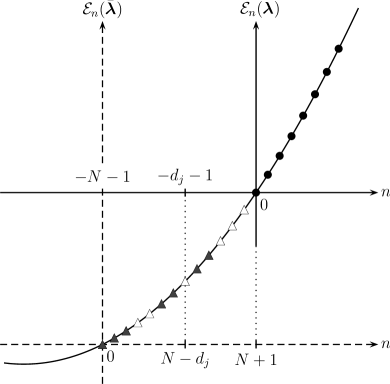
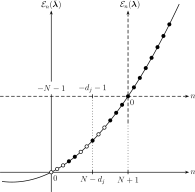
Figure 1: The left represents the Darboux-Crum transformations in terms of pseudo virtual states. The right corresponds to the Krein-Adler transformations in terms of eigenstates with shifted parameters. The black circles denote eigenstates. The white circles in the right graphic denote deleted eigenstates. The white triangles in the left graphic denote the pseudo virtual states used in the Darboux-Crum transformations in § 3.2. The black triangles denote the unused pseudo virtual states.

Let us denote the above eigenstate deleted system by $\mathcal{H}^{\text{KA}}_{\bar{\mathcal{D}}}$, $\mathcal{A}^{\text{KA}}_{\bar{\mathcal{D}}}$, $V^{\text{KA}}_{\bar{\mathcal{D}}}(x)$, etc. The general formulas of the Krein-Adler transformations [8, 9] provide:

$$\mathcal{H}^{\text{KA}}_{\bar{\mathcal{D}}}=\mathcal{A}_{\bar{\mathcal{D}}}^{\text{KA}\,\dagger}\mathcal{A}^{\text{KA}}_{\bar{\mathcal{D}}}+\mathcal{E}_{\mu}(\bar{\boldsymbol{\lambda}}),\quad\mathcal{A}^{\text{KA}}_{\bar{\mathcal{D}}}=i\bigl{(}e^{\frac{\gamma}{2}p}\sqrt{V_{\bar{\mathcal{D}}}^{\text{KA}\,*}(x)}-e^{-\frac{\gamma}{2}p}\sqrt{V^{\text{KA}}_{\bar{\mathcal{D}}}(x)}\,\bigr{)},$$

$$\phantom{\mathcal{H}^{\text{KA}}_{\bar{\mathcal{D}}}=\mathcal{A}_{\bar{\mathcal{D}}}^{\text{KA}\,\dagger}\mathcal{A}^{\text{KA}}_{\bar{\mathcal{D}}}+\mathcal{E}_{\mu}(\bar{\boldsymbol{\lambda}}),\quad}\mathcal{A}^{\text{KA}\,\dagger}_{\bar{\mathcal{D}}}=-i\bigl{(}\sqrt{V^{\text{KA}}_{\bar{\mathcal{D}}}(x)}\,e^{\frac{\gamma}{2}p}-\sqrt{V_{\bar{\mathcal{D}}}^{\text{KA}\,*}(x)}\,e^{-\frac{\gamma}{2}p}\bigr{)},$$ (3.53)

$$V^{\text{KA}}_{\bar{\mathcal{D}}}(x)=\sqrt{V(x-i\tfrac{N+1-M}{2}\gamma;\bar{\boldsymbol{\lambda}})V^{*}(x-i\tfrac{N+3-M}{2}\gamma;\bar{\boldsymbol{\lambda}})}$$

$$\phantom{V^{\text{KA}}(x)=}\times\frac{\text{W}_{\gamma}[\phi_{e_{1}},\ldots,\phi_{e_{N+1-M}}](x+i\frac{\gamma}{2};\bar{\boldsymbol{\lambda}})}{\text{W}_{\gamma}[\phi_{e_{1}},\ldots,\phi_{e_{N+1-M}}](x-i\frac{\gamma}{2};\bar{\boldsymbol{\lambda}})}\,\frac{\text{W}_{\gamma}[\phi_{e_{1}},\ldots,\phi_{e_{N+1-M}},\phi_{\mu}](x-i\gamma;\bar{\boldsymbol{\lambda}})}{\text{W}_{\gamma}[\phi_{e_{1}},\ldots,\phi_{e_{N+1-M}},\phi_{\mu}](x;\bar{\boldsymbol{\lambda}})},$$ (3.54)

$$\Phi^{\text{KA}}_{\bar{\mathcal{D}}\,n}(x)=A^{\text{KA}}_{\bar{\mathcal{D}}}(x)\text{W}_{\gamma}[\phi_{0},\phi_{1},\ldots,\breve{\phi}_{\bar{d}_{1}},\ldots,\breve{\phi}_{\bar{d}_{M}},\ldots,\phi_{N},\phi_{N+1+n}](x;\bar{\boldsymbol{\lambda}})\ \,(n=0,1,\ldots),$$ (3.55)

$$\breve{\Phi}^{\text{KA}}_{\bar{\mathcal{D}};d_{j}}(x)=A^{\text{KA}}_{\bar{\mathcal{D}}}(x)\text{W}_{\gamma}[\phi_{0},\phi_{1},\ldots,\breve{\phi}_{\bar{d}_{1}},\ldots,\phi_{\bar{d}_{j}},\ldots,\breve{\phi}_{\bar{d}_{M}},\ldots,\phi_{N}](x;\bar{\boldsymbol{\lambda}})\ (j=1,\ldots,M),\!\!\!$$ (3.56)

$$\quad A^{\text{KA}}_{\bar{\mathcal{D}}}(x)=\left(\frac{\sqrt{\prod_{j=0}^{N-M}V(x+i(\frac{s}{2}-j)\gamma;\bar{\boldsymbol{\lambda}})V^{*}(x-i(\frac{s}{2}-j)\gamma;\bar{\boldsymbol{\lambda}})}}{\text{W}_{\gamma}[\phi_{e_{1}},\ldots,\phi_{e_{N+1-M}}](x-i\frac{\gamma}{2};\bar{\boldsymbol{\lambda}})\text{W}_{\gamma}[\phi_{e_{1}},\ldots,\phi_{e_{N+1-M}}](x+i\frac{\gamma}{2};\bar{\boldsymbol{\lambda}})}\right)^{\frac{1}{2}}.$$ (3.57)

In terms of the polynomial $\bar{\Xi}_{\bar{\mathcal{D}}}$ the eigenfunctions are expressed in a similar way as (3.40)–(3.42):

$$\Phi^{\text{KA}}_{\bar{\mathcal{D}}\,n}(x)=\kappa^{\frac{1}{4}M(M-1)}\frac{\phi_{0}(x;\boldsymbol{\lambda}-M\boldsymbol{\delta})}{\sqrt{\check{\bar{\Xi}}_{\bar{\mathcal{D}}}(x-i\frac{\gamma}{2};\bar{\boldsymbol{\lambda}})\check{\bar{\Xi}}_{\bar{\mathcal{D}}}(x+i\frac{\gamma}{2};\bar{\boldsymbol{\lambda}})}}\,\check{\bar{\Xi}}_{\bar{\mathcal{D}}\,N+1+n}(x;\bar{\boldsymbol{\lambda}}),$$ (3.58)

$$\breve{\Phi}^{\text{KA}}_{\bar{\mathcal{D}};d_{j}}(x)=\kappa^{\frac{1}{4}M(M-1)}\frac{\phi_{0}(x;\boldsymbol{\lambda}-M\boldsymbol{\delta})}{\sqrt{\check{\bar{\Xi}}_{\bar{\mathcal{D}}}(x-i\frac{\gamma}{2};\bar{\boldsymbol{\lambda}})\check{\bar{\Xi}}_{\bar{\mathcal{D}}}(x+i\frac{\gamma}{2};\bar{\boldsymbol{\lambda}})}}\,\check{\bar{\Xi}}_{01\ldots\breve{\bar{d}}_{1}\ldots\bar{d}_{j}\ldots\breve{\bar{d}}_{M}\ldots N}(x;\bar{\boldsymbol{\lambda}}),$$ (3.59)

in which $\check{\bar{\Xi}}_{01\ldots\breve{\bar{d}}_{1}\ldots\bar{d}_{j}\ldots\breve{\bar{d}}_{M}\ldots N}(x;\bar{\boldsymbol{\lambda}})=\pm\check{\bar{\Xi}}_{\bar{\mathcal{D}}\,\bar{d}_{j}}(x;\bar{\boldsymbol{\lambda}})$. Let us take, without loss of generality, $d_{1}<\cdots<d_{M}$. This means that $\mu=\bar{d}_{M}$. The potential function is also expressed by the polynomials as in (3.43):

$$V^{\text{KA}}_{\bar{\mathcal{D}}}(x)=\kappa^{N+1-M}V(x;\boldsymbol{\lambda}-M\boldsymbol{\delta})\frac{\check{\bar{\Xi}}_{\bar{\mathcal{D}^{\prime}}}(x-i\gamma;\bar{\boldsymbol{\lambda}})}{\check{\bar{\Xi}}_{\bar{\mathcal{D}^{\prime}}}(x;\bar{\boldsymbol{\lambda}})}\frac{\check{\bar{\Xi}}_{\bar{\mathcal{D}}}(x+i\frac{\gamma}{2};\bar{\boldsymbol{\lambda}})}{\check{\bar{\Xi}}_{\bar{\mathcal{D}}}(x-i\frac{\gamma}{2};\bar{\boldsymbol{\lambda}})}.$$ (3.60)

The duality between the eigenstates adding and deleting transformations is stated as the following:

Proposition 1

For proper parameter ranges in which both Hamiltonians are non-singular and self-adjoint, the two systems with $\mathcal{H}_{{\mathcal{D}}}$ and $\mathcal{H}^{\text{\rm KA}}_{\bar{\mathcal{D}}}$ are equivalent. To be more specific, the equality of the Hamiltonians and the eigenfunctions read:

$$\mathcal{H}_{{\mathcal{D}}}-\mathcal{E}_{-N-1}(\boldsymbol{\lambda}) =\kappa^{-N-1}\mathcal{H}^{\text{\rm KA}}_{\bar{\mathcal{D}}},$$ (3.61)

$$\Phi_{{\mathcal{D}}\,n}(x) \propto\Phi^{\text{\rm KA}}_{\bar{\mathcal{D}}\,n}(x)\quad(n=0,1,\ldots),$$ (3.62)

$$\breve{\Phi}_{{\mathcal{D}};d_{j}}(x) \propto\breve{\Phi}^{\text{\rm KA}}_{\bar{\mathcal{D}};d_{j}}(x)\quad(j=1,2,\ldots,M).$$ (3.63)

The singularity free conditions of the potential are [7, 9]

$$\prod_{j=1}^{N+1-M}(n-e_{j})\geq 0\quad(\,\forall n\in\mathbb{Z}_{\geq 0}).$$ (3.64)

The parameters of the shifted Hamiltonian $\mathcal{H}^{\text{KA}}_{\bar{\mathcal{D}}}$ are constrained by the self-adjointness. For the Wilson and Askey-Wilson cases, they are

$$\text{W}:\ \text{Re}\,a_{j}>\tfrac{1}{2}(N+1),\quad\text{AW}:\ |a_{j}|<q^{\frac{1}{2}(N+1)}\quad(j=1,\ldots,4),$$ (3.65)

generalising (3.17). The two relations (3.62) and (3.63) imply the relationships among polynomials:

$$P_{\mathcal{D},n}(\eta;\boldsymbol{\lambda}) \propto\bar{\Xi}_{\bar{\mathcal{D}}\,N+1+n}(\eta;\bar{\boldsymbol{\lambda}})\quad(n=0,1,\ldots),$$ (3.66)

$$\Xi_{d_{1}\ldots\breve{d}_{j}\ldots d_{M}}(\eta;\boldsymbol{\lambda}) \propto\bar{\Xi}_{\bar{\mathcal{D}}\,\bar{d}_{j}}(\eta;\bar{\boldsymbol{\lambda}})\quad(j=1,2,\ldots,M).$$ (3.67)

3.4 Derivation of the Casoratian identities

The above duality, i.e. Proposition 1, is the simple consequence of the following

Proposition 2

The Casoratian Identities read

$$\Xi_{\mathcal{D}}(\eta;\boldsymbol{\lambda})\propto\bar{\Xi}_{\bar{\mathcal{D}}}(\eta;\bar{\boldsymbol{\lambda}}),$$ (3.68)

namely,

$$\quad\varphi_{M}(x)^{-1}\,\text{\rm W}_{\gamma}[\check{\xi}_{d_{1}},\check{\xi}_{d_{2}},\ldots,\check{\xi}_{d_{M}}](x;\boldsymbol{\lambda})$$

$$\propto\varphi_{N+1-M}(x)^{-1}\,\text{\rm W}_{\gamma}[\check{P}_{0},\check{P}_{1},\ldots,\breve{\check{P}}_{\bar{d}_{1}},\ldots,\breve{\check{P}}_{\bar{d}_{M}},\ldots,\check{P}_{N}](x;\bar{\boldsymbol{\lambda}}).$$ (3.69)

Recall that $\check{\xi}_{\text{v}}(x;\boldsymbol{\lambda})=\check{P}_{\text{v}}\bigl{(}x;\mathfrak{t}(\boldsymbol{\lambda})\bigr{)}$. This proposition shows the relation between Casoratians of polynomials of twisted and shifted parameters. It is straightforward to show the equality of the Hamiltonians (3.61) based on the expressions of the potential functions (3.43), (3.60) and $\Xi_{\mathcal{D}}\propto\bar{\Xi}_{\bar{\mathcal{D}}}$ (3.68). The proportionalities of the eigenfunctions (3.62) and (3.63) follow from the equality of the Hamiltonians, so long as the Hamiltonians are non-singular and self-adjoint. The inductive proof of Proposition 2 in $M$ consists of two steps, as is the case for the proof of the Wronskian identities in [1].

first step : As a first step we prove (3.68) for $M=1$, $N\geq d_{1}\equiv\text{v}$, that is $\mathcal{D}=\{\text{v}\}$, $\bar{\mathcal{D}}=\{0,1,\ldots,\breve{\bar{\text{v}}},\ldots,N\}$ (see Fig. 2):

$$\xi_{\text{v}}(\eta;\boldsymbol{\lambda})\propto\bar{\Xi}_{\bar{\mathcal{D}}}(\eta;\bar{\boldsymbol{\lambda}}).$$ (3.70)

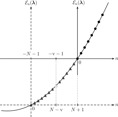
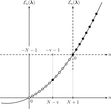
Figure 2: The symbols are the same as those in Fig. 1. By shape invariance, deleting the ground state $\bar{\text{v}}=N-\text{v}$ from $\mathcal{H}^{\text{KA}}_{\bar{\mathcal{D}}}$ leads to the undeformed system $\mathcal{H}(\boldsymbol{\lambda})$.

Let us consider a Hamiltonian system $\bar{\mathcal{H}}$ obtained from $\mathcal{H}^{\text{KA}}_{\bar{\mathcal{D}}}$ by deleting its ground state $\bar{\text{v}}=N-\text{v}$:

$$\bar{\mathcal{H}}=\mathcal{A}^{\text{KA}}_{\bar{\mathcal{D}}}\mathcal{A}_{\bar{\mathcal{D}}}^{\text{KA}\,\dagger}+\mathcal{E}_{\bar{\text{v}}}(\bar{\boldsymbol{\lambda}}),$$

$$\bar{\mathcal{H}}\Phi^{\prime}_{n}(x)=\mathcal{E}_{n}(\bar{\boldsymbol{\lambda}})\Phi^{\prime}_{n}(x)\quad(n\geq N+1).$$

By shape invariance, the ground state ($n=N+1$) of $\bar{\mathcal{H}}$ coincides with that of the undeformed system $\mathcal{H}(\boldsymbol{\lambda})$, i.e. $\phi_{0}(x;\boldsymbol{\lambda})$:

$$\bar{\mathcal{H}}\phi_{0}(x;\boldsymbol{\lambda})=\mathcal{E}_{N+1}(\bar{\boldsymbol{\lambda}})\phi_{0}(x;\boldsymbol{\lambda}).$$

In this case $\bar{\mathcal{D}}^{\prime}=\{0,1,\ldots,N\}$ and $\check{\bar{\Xi}}_{\{0,1,\ldots,N\}}(x;\bar{\boldsymbol{\lambda}})=\text{constant}$ (3.47), we obtain from (3.60)

$$V^{\text{KA}}_{\bar{\mathcal{D}}}(x)=\kappa^{N}V(x;\boldsymbol{\lambda}-\boldsymbol{\delta})\frac{\check{\bar{\Xi}}_{\bar{\mathcal{D}}}(x+i\frac{\gamma}{2};\bar{\boldsymbol{\lambda}})}{\check{\bar{\Xi}}_{\bar{\mathcal{D}}}(x-i\frac{\gamma}{2};\bar{\boldsymbol{\lambda}})},$$

and

$$\bar{\mathcal{H}} =\kappa^{N}\Bigl{(}\sqrt{V(x-i\tfrac{\gamma}{2};\boldsymbol{\lambda}-\boldsymbol{\delta})V^{*}(x-i\tfrac{\gamma}{2};\boldsymbol{\lambda}-\boldsymbol{\delta})}\,e^{\gamma p}$$

$$\phantom{=\kappa^{N}\Bigl{(}}+\sqrt{V(x+i\tfrac{\gamma}{2};\boldsymbol{\lambda}-\boldsymbol{\delta})V^{*}(x+i\tfrac{\gamma}{2};\boldsymbol{\lambda}-\boldsymbol{\delta})}\,e^{-\gamma p}$$

$$\phantom{=\kappa^{N}\Bigl{(}}-V(x+i\tfrac{\gamma}{2};\boldsymbol{\lambda}-\boldsymbol{\delta})\frac{\check{\bar{\Xi}}_{\bar{\mathcal{D}}}(x+i\gamma;\bar{\boldsymbol{\lambda}})}{\check{\bar{\Xi}}_{\bar{\mathcal{D}}}(x;\bar{\boldsymbol{\lambda}})}-V^{*}(x-i\tfrac{\gamma}{2};\boldsymbol{\lambda}-\boldsymbol{\delta})\frac{\check{\bar{\Xi}}_{\bar{\mathcal{D}}}(x-i\gamma;\bar{\boldsymbol{\lambda}})}{\check{\bar{\Xi}}_{\bar{\mathcal{D}}}(x;\bar{\boldsymbol{\lambda}})}\Bigr{)}+\mathcal{E}_{\bar{\text{v}}}(\bar{\boldsymbol{\lambda}}).$$

By using the zero mode equation (2.30), the shape covariance relations of $\phi_{0}$ (2.39)–(2.40) and of $V$ (2.37) and the general twisting relation (2.63), we obtain

$$0 =\bigl{(}\bar{\mathcal{H}}-\mathcal{E}_{N+1}(\bar{\boldsymbol{\lambda}})\bigr{)}\phi_{0}(x;\boldsymbol{\lambda})$$

$$=\kappa^{N+1}\Bigl{(}V(x;\boldsymbol{\lambda})+V^{*}(x;\boldsymbol{\lambda})$$

$$\phantom{=\kappa^{N+1}\Bigl{(}}-\alpha(\boldsymbol{\lambda})V^{*}\bigl{(}x;\mathfrak{t}(\boldsymbol{\lambda})\bigr{)}\frac{\check{\bar{\Xi}}_{\bar{\mathcal{D}}}(x+i\gamma;\bar{\boldsymbol{\lambda}})}{\check{\bar{\Xi}}_{\bar{\mathcal{D}}}(x;\bar{\boldsymbol{\lambda}})}-\alpha(\boldsymbol{\lambda})V\bigl{(}x;\mathfrak{t}(\boldsymbol{\lambda})\bigr{)}\frac{\check{\bar{\Xi}}_{\bar{\mathcal{D}}}(x-i\gamma;\bar{\boldsymbol{\lambda}})}{\check{\bar{\Xi}}_{\bar{\mathcal{D}}}(x;\bar{\boldsymbol{\lambda}})}\Bigr{)}\phi_{0}(x;\boldsymbol{\lambda})$$

$$\quad+\bigl{(}\mathcal{E}_{\bar{\text{v}}}(\bar{\boldsymbol{\lambda}})-\mathcal{E}_{N+1}(\bar{\boldsymbol{\lambda}})\bigr{)}\phi_{0}(x;\boldsymbol{\lambda}).$$ (3.71)

With the second basic twist relation (2.43), the properties of $\mathcal{E}_{n}$ (3.50)–(3.51) and $\alpha^{\prime}(\boldsymbol{\lambda})=\mathcal{E}_{-1}(\boldsymbol{\lambda})$, we obtain a difference equation for $\check{\bar{\Xi}}_{\bar{\mathcal{D}}}(x;\bar{\boldsymbol{\lambda}})$:

$$V\bigl{(}x;\mathfrak{t}(\boldsymbol{\lambda})\bigr{)}\bigl{(}\check{\bar{\Xi}}_{\bar{\mathcal{D}}}(x-i\gamma;\bar{\boldsymbol{\lambda}})-\check{\bar{\Xi}}_{\bar{\mathcal{D}}}(x;\bar{\boldsymbol{\lambda}})\bigr{)}+V^{*}\bigl{(}x;\mathfrak{t}(\boldsymbol{\lambda})\bigr{)}\bigl{(}\check{\bar{\Xi}}_{\bar{\mathcal{D}}}(x+i\gamma;\bar{\boldsymbol{\lambda}})-\check{\bar{\Xi}}_{\bar{\mathcal{D}}}(x;\bar{\boldsymbol{\lambda}})\bigr{)}$$

$$=\mathcal{E}_{\text{v}}\bigl{(}\mathfrak{t}(\boldsymbol{\lambda})\bigr{)}\check{\bar{\Xi}}_{\bar{\mathcal{D}}}(x;\bar{\boldsymbol{\lambda}}).$$ (3.72)

This is indeed the difference equation for $P_{\text{v}}\bigl{(}\eta(x);\mathfrak{t}(\boldsymbol{\lambda})\bigr{)}$ and we arrive at the relation $P_{\text{v}}\bigl{(}\eta;\mathfrak{t}(\boldsymbol{\lambda})\bigr{)}\propto\bar{\Xi}_{\bar{\mathcal{D}}}(\eta;\bar{\boldsymbol{\lambda}})$ (3.70).

second step : Assume that (3.69) holds till $M$ ($M\geq 1$), we will show that it also holds for $M+1$.

By using the Casoratian identity (3.4), we obtain

$$\quad\text{W}_{\gamma}[\check{\xi}_{d_{1}},\ldots,\check{\xi}_{d_{M-1}}](x;\boldsymbol{\lambda})\cdot\text{W}_{\gamma}[\check{\xi}_{d_{1}},\ldots,\check{\xi}_{d_{M-1}},\check{\xi}_{d_{M}},\check{\xi}_{d_{M+1}}](x;\boldsymbol{\lambda})$$

$$=\text{W}_{\gamma}\bigl{[}\text{W}_{\gamma}[\check{\xi}_{d_{1}},\ldots,\check{\xi}_{d_{M-1}},\check{\xi}_{d_{M}}],\text{W}_{\gamma}[\check{\xi}_{d_{1}},\ldots,\check{\xi}_{d_{M-1}},\check{\xi}_{d_{M+1}}]\bigr{]}(x;\boldsymbol{\lambda})$$

$$\propto\text{W}_{\gamma}\Bigl{[}\frac{\varphi_{M}(x)}{\varphi_{N+1-M}(x)}\text{W}_{\gamma}[\check{P}_{0},\ldots,\breve{\check{P}}_{\bar{d}_{1}},\ldots,\breve{\check{P}}_{\bar{d}_{M-1}},\ldots,\breve{\check{P}}_{\bar{d}_{M}},\ldots,\check{P}_{N}],$$

$$\phantom{\propto\text{W}_{\gamma}\Bigl{[}}\ \frac{\varphi_{M}(x)}{\varphi_{N+1-M}(x)}\text{W}_{\gamma}[\check{P}_{0},\ldots,\breve{\check{P}}_{\bar{d}_{1}},\ldots,\breve{\check{P}}_{\bar{d}_{M-1}},\ldots,\breve{\check{P}}_{\bar{d}_{M+1}},\ldots,\check{P}_{N}]\Bigr{]}(x;\bar{\boldsymbol{\lambda}})$$

$$=\frac{\varphi_{M}(x+i\frac{\gamma}{2})}{\varphi_{N+1-M}(x+i\frac{\gamma}{2})}\frac{\varphi_{M}(x-i\frac{\gamma}{2})}{\varphi_{N+1-M}(x-i\frac{\gamma}{2})}$$

$$\qquad\times\text{W}_{\gamma}\bigl{[}\text{W}_{\gamma}[\check{P}_{0},\ldots,\breve{\check{P}}_{\bar{d}_{1}},\ldots,\breve{\check{P}}_{\bar{d}_{M-1}},\ldots,\breve{\check{P}}_{\bar{d}_{M}},\ldots,\check{P}_{N}],$$

$$\phantom{\qquad\times\text{W}_{\gamma}\bigl{[}}\ \ \text{W}_{\gamma}[\check{P}_{0},\ldots,\breve{\check{P}}_{\bar{d}_{1}},\ldots,\breve{\check{P}}_{\bar{d}_{M-1}},\ldots,\breve{\check{P}}_{\bar{d}_{M+1}},\ldots,\check{P}_{N}]\bigr{]}(x;\bar{\boldsymbol{\lambda}})$$

$$=\pm\frac{\varphi_{M}(x+i\frac{\gamma}{2})}{\varphi_{N+1-M}(x+i\frac{\gamma}{2})}\frac{\varphi_{M}(x-i\frac{\gamma}{2})}{\varphi_{N+1-M}(x-i\frac{\gamma}{2})}$$

$$\qquad\times\text{W}_{\gamma}[\check{P}_{0},\ldots,\breve{\check{P}}_{\bar{d}_{1}},\ldots,\breve{\check{P}}_{\bar{d}_{M-1}},\ldots,\breve{\check{P}}_{\bar{d}_{M}},\ldots,\breve{\check{P}}_{\bar{d}_{M+1}},\ldots,\check{P}_{N}](x;\bar{\boldsymbol{\lambda}})$$

$$\qquad\times\text{W}_{\gamma}[\check{P}_{0},\ldots,\breve{\check{P}}_{\bar{d}_{1}},\ldots,\breve{\check{P}}_{\bar{d}_{M-1}},\ldots,\check{P}_{N}](x;\bar{\boldsymbol{\lambda}})$$

$$\propto\frac{\varphi_{M}(x+i\frac{\gamma}{2})}{\varphi_{N+1-M}(x+i\frac{\gamma}{2})}\frac{\varphi_{M}(x-i\frac{\gamma}{2})}{\varphi_{N+1-M}(x-i\frac{\gamma}{2})}\frac{\varphi_{N+2-M}(x)}{\varphi_{M-1}(x)}$$

$$\qquad\times\text{W}_{\gamma}[\check{P}_{0},\ldots,\breve{\check{P}}_{\bar{d}_{1}},\ldots,\breve{\check{P}}_{\bar{d}_{M+1}},\ldots,\check{P}_{N}](x;\bar{\boldsymbol{\lambda}})\cdot\text{W}_{\gamma}[\check{\xi}_{d_{1}},\ldots,\check{\xi}_{d_{M-1}}](x;\boldsymbol{\lambda}).$$

This leads to

$$\quad\varphi_{M+1}(x)^{-1}\,\text{W}_{\gamma}[\check{\xi}_{d_{1}},\ldots,\check{\xi}_{d_{M+1}}](x;\boldsymbol{\lambda})$$

$$\propto\varphi_{N-M}(x)^{-1}\,\text{W}_{\gamma}[\check{P}_{0},\ldots,\breve{\check{P}}_{\bar{d}_{1}},\ldots,\breve{\check{P}}_{\bar{d}_{M+1}},\ldots,\check{P}_{N}](x;\bar{\boldsymbol{\lambda}})$$

$$\qquad\times\frac{\varphi_{M}(x+i\frac{\gamma}{2})}{\varphi_{N+1-M}(x+i\frac{\gamma}{2})}\frac{\varphi_{M}(x-i\frac{\gamma}{2})}{\varphi_{N+1-M}(x-i\frac{\gamma}{2})}\frac{\varphi_{N+2-M}(x)}{\varphi_{M-1}(x)}\frac{\varphi_{N-M}(x)}{\varphi_{M+1}(x)}$$

$$\propto\varphi_{N-M}(x)^{-1}\,\text{W}_{\gamma}[\check{P}_{0},\ldots,\breve{\check{P}}_{\bar{d}_{1}},\ldots,\breve{\check{P}}_{\bar{d}_{M+1}},\ldots,\check{P}_{N}](x;\bar{\boldsymbol{\lambda}}),$$

namely $M+1$ case is shown. Here we have used

$$\varphi_{M}(x+i\tfrac{\gamma}{2})\varphi_{M}(x-i\tfrac{\gamma}{2})=\frac{\varphi_{M-1}(x)\varphi_{M+1}(x)}{\varphi(x)}\quad(M\geq 1),$$ (3.73)

which is easily verified. This concludes the induction proof of (3.69).

4 Reduced Case Polynomials

It is well known that the other members of the Askey scheme polynomials can be obtained by reductions from the Wilson and the Askey-Wilson polynomials. Here we list the discrete symmetry transformations and the pseudo virtual state wave functions for all the reduced case polynomials. In contrast to the virtual state wave functions, the pseudo virtual state wave functions are universal and they exist for all the solvable potentials with shape invariance. For example, for the systems of the harmonic oscillator and the $q$-harmonic oscillator with the ($q$-)Hermite polynomials as the main part of the eigenfunctions [19], virtual state wave functions do not exist. However, the pseudo virtual state wave functions for the harmonic oscillator was reported in [1] and those for the $q$-harmonic oscillator will be introduced in § 4.2. The Casoratian identities hold for these reduced case polynomials, too.

4.1 Reductions from the Wilson polynomial

Three polynomials belong to this group; the continuous dual Hahn (cdH), the continuous Hahn (cH) and the Meixner-Pollaczek (MP) polynomials. They are obtained from the Wilson polynomial by some limiting procedures [4]. The discrete symmetries are also obtained by the same limiting procedures from that of the Wilson polynomial. It should be noted that the Wilson polynomial is also obtained from the Askey-Wilson polynomial by a certain limiting procedure [4].

The defining domain and the parameters of these reduced case polynomials are:

$$\text{cdH}:\ \ x_{1}=0,\ \ x_{2}=\infty,\quad \gamma=1, \boldsymbol{\lambda}=(a_{1},a_{2},a_{3}), \boldsymbol{\delta}=(\tfrac{1}{2},\tfrac{1}{2},\tfrac{1}{2}),\quad \kappa=1,$$

$$\text{cH}:\ \ x_{1}=-\infty,\ \ x_{2}=\infty,\quad \gamma=1, \boldsymbol{\lambda}=(a_{1},a_{2}), \boldsymbol{\delta}=(\tfrac{1}{2},\tfrac{1}{2}),\quad \kappa=1,$$

$$\text{MP}:\ \ x_{1}=-\infty,\ \ x_{2}=\infty,\quad \gamma=1, \boldsymbol{\lambda}=(a,\phi), \boldsymbol{\delta}=(\tfrac{1}{2},0),\quad \kappa=1,$$ (4.1)

in which the parameters are restricted by

$$\text{cdH}: \ \ \{a_{1}^{*},a_{2}^{*},a_{3}^{*}\}=\{a_{1},a_{2},a_{3}\}\ \ (\text{as a set});\quad\text{Re}\,a_{i}>0,$$

$$\text{cH}: \ \ \text{Re}\,a_{i}>0;\quad(a_{3},a_{4})\stackrel{{\scriptstyle\text{def}}}{{=}}(a_{1}^{*},a_{2}^{*}),$$

$$\text{MP}: \ \ a>0,\quad 0<\phi<\pi.$$ (4.2)

Here are the fundamental data:

$$V(x;\boldsymbol{\lambda}) =\left\{\begin{array}[]{ll}\bigl{(}2ix(2ix+1)\bigr{)}^{-1}\prod_{j=1}^{3}(a_{j}+ix)&:\text{cdH}\\[4.0pt] \prod_{j=1}^{2}(a_{j}+ix)&:\text{cH}\\[4.0pt] e^{i(\frac{\pi}{2}-\phi)}(a+ix)&:\text{MP}\end{array}\right.,$$ (4.6)

$$\eta(x) =\left\{\begin{array}[]{ll}x^{2}&:\text{cdH}\\ x&:\text{cH,\,MP}\end{array}\right.,\quad\varphi(x)=\left\{\begin{array}[]{ll}2x&:\text{cdH}\\ 1&:\text{cH,\,MP}\end{array}\right.,$$ (4.11)

$$\mathcal{E}_{n}(\boldsymbol{\lambda}) =\left\{\begin{array}[]{ll}n&:\text{cdH}\\ n(n+b_{1}-1),\quad b_{1}\stackrel{{\scriptstyle\text{def}}}{{=}}a_{1}+a_{2}+a_{3}+a_{4},&:\text{cH}\\[2.0pt] 2n\sin\phi&:\text{MP}\end{array}\right.,$$ (4.15)

$$\phi_{n}(x;\boldsymbol{\lambda}) =\phi_{0}(x;\boldsymbol{\lambda})\check{P}_{n}(x;\boldsymbol{\lambda}),$$ (4.16)

$$\check{P}_{n}(x;\boldsymbol{\lambda}) =P_{n}\bigl{(}\eta(x);\boldsymbol{\lambda}\bigr{)}=\left\{\begin{array}[]{ll}S_{n}\bigl{(}\eta(x);a_{1},a_{2},a_{3}\bigr{)}&:\text{cdH}\\[1.0pt] p_{n}\bigl{(}\eta(x);a_{1},a_{2},a_{3},a_{4}\bigr{)}&:\text{cH}\\[2.0pt] P_{n}^{(a)}\bigl{(}\eta(x);\phi\bigr{)}&:\text{MP}\end{array}\right.$$ (4.20)

$$=\left\{\begin{array}[]{ll}{\displaystyle(a_{1}+a_{2},a_{1}+a_{3})_{n}\ {}_{3}F_{2}\Bigl{(}\genfrac{}{}{0.0pt}{}{-n,\,a_{1}+ix,\,a_{1}-ix}{a_{1}+a_{2},\,a_{1}+a_{3}}\Bigm{|}1\Bigr{)}}&:\text{cdH}\\[8.0pt] {\displaystyle i^{n}\frac{(a_{1}+a_{3},a_{1}+a_{4})_{n}}{n!}\ {}_{3}F_{2}\Bigl{(}\genfrac{}{}{0.0pt}{}{-n,\,n+b_{1}-1,\,a_{1}+ix}{a_{1}+a_{3},\,a_{1}+a_{4}}\!\Bigm{|}\!1\Bigr{)}}&:\text{cH}\\[8.0pt] {\displaystyle\frac{(2a)_{n}}{n!}\,e^{in\phi}{}_{2}F_{1}\Bigl{(}\genfrac{}{}{0.0pt}{}{-n,\,a+ix}{2a}\Bigm{|}1-e^{-2i\phi}\Bigr{)}}&:\text{MP}\end{array}\right.,$$ (4.24)

$$\phi_{0}(x;\boldsymbol{\lambda}) =\left\{\begin{array}[]{ll}\sqrt{(\Gamma(2ix)\Gamma(-2ix))^{-1}\prod_{j=1}^{3}\Gamma(a_{j}+ix)\Gamma(a_{j}-ix)}&:\text{cdH}\\[6.0pt] \sqrt{\Gamma(a_{1}+ix)\Gamma(a_{2}+ix)\Gamma(a_{3}-ix)\Gamma(a_{4}-ix)}&:\text{cH}\\[6.0pt] e^{(\phi-\frac{\pi}{2})x}\sqrt{\Gamma(a+ix)\Gamma(a-ix)}&:\text{MP}\end{array}\right.,$$ (4.28)

$$f_{n}(\boldsymbol{\lambda})=\left\{\begin{array}[]{ll}-n&:\text{cdH}\\ n+b_{1}-1&:\text{cH}\\ 2\sin\phi&:\text{MP}\end{array}\right.,\quad b_{n-1}(\boldsymbol{\lambda})=\left\{\begin{array}[]{ll}-1&:\text{cdH}\\ n&:\text{cH}\\ n&:\text{MP}\end{array}\right..$$ (4.35)

The relations (2.37)–(2.38) are satisfied.

4.1.1 pseudo virtual state wave functions

The twisting of the polynomials in this group is straightforward. We define the twisted potential $V^{\prime}(x;\boldsymbol{\lambda})$ (2.41) by

$$\mathfrak{t}(\boldsymbol{\lambda}) =\left\{\begin{array}[]{ll}(1-a_{1},1-a_{2},1-a_{3})&:\text{cdH}\\ (1-a_{1}^{*},1-a_{2}^{*})&:\text{cH}\\ (1-a,\pi-\phi)&:\text{MP}\\ \end{array}\right.,\quad\mathfrak{t}^{2}=\text{Id}.$$ (4.39)

The relations (2.42)–(2.43), (2.49) and (2.63) are satisfied with

$$\alpha(\boldsymbol{\lambda})=\left\{\begin{array}[]{ll}-1&:\text{cdH,\,MP}\\ 1&:\text{cH}\end{array}\right.,\qquad\alpha^{\prime}(\boldsymbol{\lambda})=\mathcal{E}_{-1}(\boldsymbol{\lambda})=\left\{\begin{array}[]{ll}-1&:\text{cdH}\\ 2-b_{1}&:\text{cH}\\ -2\sin\phi&:\text{MP}\end{array}\right.,$$ (4.45)

and the pseudo virtual state wave function is obtained by simple twisting of the parameters $\tilde{\phi}_{\text{v}}(x;\boldsymbol{\lambda})=\tilde{\phi}_{0}(x;\boldsymbol{\lambda})\check{\xi}_{\text{v}}(x;\boldsymbol{\lambda})$ as in (2.61)–(2.62).

4.2 Reductions from the Askey-Wilson polynomial

There are two groups, to be called (A) and (B), of polynomials obtained by two different types of reductions from the Askey-Wilson polynomial. Group (A), consisting of one polynomial, is obtained by specifying the four parameters $(a_{1},a_{2},a_{3},a_{4})$ of the Askey-Wilson polynomial, as simple functions of two ($\alpha$ and $\beta$) parameters. Group (B), consisting of five polynomials, is obtained by setting some of the parameters $\{a_{j}\}$ to zero. For all member polynomials in this subsection, we have

$$x_{1}=0,\quad x_{2}=\pi,\quad\gamma=\log q,\quad\kappa=q^{-1},\quad\eta(x)=\cos x,\quad\varphi(x)=2\sin x.$$

4.2.1 Group (A) reductions from the Askey-Wilson polynomial

The continuous $q$-Jacobi (c$q$J) polynomial belongs to this group. It is obtained by restricting the four parameters $(a_{1},a_{2},a_{3},a_{4})$ of the Askey-Wilson polynomial as

$$(a_{1},a_{2},a_{3},a_{4})=\bigl{(}q^{\frac{1}{2}(\alpha+\frac{1}{2})},q^{\frac{1}{2}(\alpha+\frac{3}{2})},-q^{\frac{1}{2}(\beta+\frac{1}{2})},-q^{\frac{1}{2}(\beta+\frac{3}{2})}\bigr{)},$$ (4.46)

$$\boldsymbol{\lambda}=(\alpha,\beta),\quad\boldsymbol{\delta}=(1,1),\quad\alpha,\beta\geq-\tfrac{1}{2},$$ (4.47)

$$V(x\,;\boldsymbol{\lambda})=\frac{(1-q^{\frac{1}{2}(\alpha+\frac{1}{2})}e^{ix})(1-q^{\frac{1}{2}(\alpha+\frac{3}{2})}e^{ix})(1+q^{\frac{1}{2}(\beta+\frac{1}{2})}e^{ix})(1+q^{\frac{1}{2}(\beta+\frac{3}{2})}e^{ix})}{(1-e^{2ix})(1-qe^{2ix})}.$$ (4.48)

The eigenvalues and the corresponding eigenfunctions are:

$$\mathcal{E}_{n}(\boldsymbol{\lambda}) =(q^{-n}-1)(1-q^{n+\alpha+\beta+1}),$$ (4.49)

$$\check{P}_{n}(x;\boldsymbol{\lambda}) =P_{n}\bigl{(}\eta(x);\boldsymbol{\lambda}\bigr{)}=P_{n}^{(\alpha,\beta)}\bigl{(}\eta(x)|q\bigr{)}$$

$$=\frac{(q^{\alpha+1}\,;q)_{n}}{(q\,;q)_{n}}\,{}_{4}\phi_{3}\Bigl{(}\genfrac{}{}{0.0pt}{}{q^{-n},\,q^{n+\alpha+\beta+1},\,q^{\frac{1}{2}(\alpha+\frac{1}{2})}e^{ix},\,q^{\frac{1}{2}(\alpha+\frac{1}{2})}e^{-ix}}{q^{\alpha+1},\,-q^{\frac{1}{2}(\alpha+\beta+1)},\,-q^{\frac{1}{2}(\alpha+\beta+2)}}\Bigm{|}q\,;q\Bigr{)},$$ (4.50)

$$\phi_{0}(x\,;\boldsymbol{\lambda}) =\sqrt{\frac{(e^{2ix},e^{-2ix}\,;q)_{\infty}}{(q^{\frac{1}{2}(\alpha+\frac{1}{2})}e^{ix},-q^{\frac{1}{2}(\beta+\frac{1}{2})}e^{ix},q^{\frac{1}{2}(\alpha+\frac{1}{2})}e^{-ix},-q^{\frac{1}{2}(\beta+\frac{1}{2})}e^{-ix}\,;q^{\frac{1}{2}})_{\infty}}},$$ (4.51)

$$f_{n}(\boldsymbol{\lambda}) =\frac{q^{\frac{1}{2}(\alpha+\frac{3}{2})}q^{-n}(1-q^{n+\alpha+\beta+1})}{(1+q^{\frac{1}{2}(\alpha+\beta+1)})(1+q^{\frac{1}{2}(\alpha+\beta+2)})},$$ (4.52)

$$b_{n-1}(\boldsymbol{\lambda}) =q^{-\frac{1}{2}(\alpha+\frac{3}{2})}q^{n}(q^{-n}-1)(1+q^{\frac{1}{2}(\alpha+\beta+1)})(1+q^{\frac{1}{2}(\alpha+\beta+2)}).$$ (4.53)

The relations (2.37)–(2.38) are satisfied.

4.2.2 pseudo virtual states for Group (A)

The twisting of the Askey-Wilson case (2.52) is consistent with the reduction to Group (A). That is $a_{j}\to q\,a_{j}^{-1}$ ($j=1,\ldots,4$) simply translates to the twisting of the two parameters $\alpha$ and $\beta$:

$$\mathfrak{t}(\alpha,\beta)=(-\alpha,-\beta),\quad\mathfrak{t}^{2}=\text{Id},$$ (4.54)

giving the potential $V^{\prime}(x;\boldsymbol{\lambda})$ (2.41). The relations (2.42)–(2.43), (2.49) and (2.63) are satisfied with

$$\alpha(\boldsymbol{\lambda})=q^{\alpha+\beta},\quad\alpha^{\prime}(\boldsymbol{\lambda})=\mathcal{E}_{-1}(\boldsymbol{\lambda})=(q-1)(1-q^{\alpha+\beta}),$$ (4.55)

and the pseudo virtual state wave function is obtained by simple twisting of the parameters $\tilde{\phi}_{\text{v}}(x;\boldsymbol{\lambda})=\tilde{\phi}_{0}(x;\boldsymbol{\lambda})\check{\xi}_{\text{v}}(x;\boldsymbol{\lambda})$ as in (2.61)–(2.62).

4.2.3 Group (B) reductions from the Askey-Wilson polynomial

Five polynomials belong to Group (B); the continuous dual $q$-Hahn (cd$q$H), Al-Salam-Chihara (ASC), continuous big $q$-Hermite (cb$q$H), continuous $q$-Hermite (c$q$H) and continuous $q$-Laguerre (c$q$L) polynomials. The first four members are obtained by setting $a_{4}=0$ for cd$q$H, $a_{4}=a_{3}=0$ for ASC, $a_{4}=a_{3}=a_{2}=0$ for cb$q$H and $a_{4}=a_{3}=a_{2}=a_{1}=0$ for c$q$H. The c$q$L is obtained by setting $a_{4}=a_{3}=0$ of the continuous $q$-Jacobi case. In other words, the c$q$L is obtained by taking the limit $\beta\to+\infty$ of the continuous $q$-Jacobi case. The parameters of Group (B) are

$$\text{cd$q$H}:\ \ \boldsymbol{\lambda}=(\lambda_{1},\lambda_{2},\lambda_{3}),\quad q^{\boldsymbol{\lambda}}=(a_{1},a_{2},a_{3}),\quad \boldsymbol{\delta}=(\tfrac{1}{2},\tfrac{1}{2},\tfrac{1}{2}),\quad |a_{j}|<1,$$ (4.56)

$$\text{ASC}:\ \ \boldsymbol{\lambda}=(\lambda_{1},\lambda_{2}),\quad q^{\boldsymbol{\lambda}}=(a_{1},a_{2}),\quad \boldsymbol{\delta}=(\tfrac{1}{2},\tfrac{1}{2}),\quad |a_{j}|<1,$$ (4.57)

$$\text{cb$q$H}:\ \ \boldsymbol{\lambda}=\lambda_{1},\quad q^{\boldsymbol{\lambda}}=a_{1}=a,\quad \boldsymbol{\delta}=\tfrac{1}{2},\quad |a|<1,$$ (4.58)

$$\text{c$q$H}:\ \ \boldsymbol{\lambda}:\ \text{none},$$ (4.59)

$$\text{c$q$L}:\ \ \boldsymbol{\lambda}=\alpha, \boldsymbol{\delta}=1,\quad \alpha>-\tfrac{1}{2}.$$ (4.60)

The basic data are obtained from those of the Askey-Wilson and the continuous $q$-Jacobi polynomials by simply putting the appropriate parameters to zero:

$$V(x;\boldsymbol{\lambda},q)=\frac{1}{(1-e^{2ix})(1-qe^{2ix})}\times\left\{\begin{array}[]{l}\prod_{j=1}^{m}(1-a_{j}e^{ix})\qquad\qquad:m=3,2,1,0\\[6.0pt] (1-q^{\frac{1}{2}(\alpha+\frac{1}{2})}e^{ix})(1-q^{\frac{1}{2}(\alpha+\frac{3}{2})}e^{ix})\ \ :\text{c$q$L}\end{array}\right.,$$ (4.63)

$$\mathcal{E}_{n}(\boldsymbol{\lambda})=q^{-n}-1,$$ (4.64)

$$\phi_{0}(x;\boldsymbol{\lambda})=\sqrt{(e^{2ix},e^{-2ix}\,;q)_{\infty}}\times\left\{\begin{array}[]{l}\sqrt{\prod_{j=1}^{m}(a_{j}e^{ix},a_{j}e^{-ix}\,;q)_{\infty}^{-1}}\quad\ :m=3,2,1,0\\[6.0pt] \sqrt{(q^{\frac{1}{2}(\alpha+\frac{1}{2})}e^{ix},q^{\frac{1}{2}(\alpha+\frac{1}{2})}e^{-ix}\,;q^{\frac{1}{2}})_{\infty}^{-1}}\ \ :\text{c$q$L}\end{array}\right.,$$ (4.67)

$$\check{P}_{n}(x;\boldsymbol{\lambda})=P_{n}\bigl{(}\eta(x);\boldsymbol{\lambda}\bigr{)}=\left\{\begin{array}[]{ll}p_{n}\bigl{(}\eta(x);a_{1},a_{2},a_{3}|q\bigr{)}&:\text{cd$q$H}\\ Q_{n}\bigl{(}\eta(x);a_{1},a_{2}|q\bigr{)}&:\text{ASC}\\ H_{n}\bigl{(}\eta(x);a|q\bigr{)}&:\text{cb$q$H}\\ H_{n}\bigl{(}\eta(x)|q\bigr{)}&:\text{c$q$H}\\ P_{n}^{(\alpha)}\bigl{(}\eta(x)|q\bigr{)}&:\text{c$q$L}\end{array}\right.$$ (4.73)

$$\phantom{\check{P}_{n}(x;\boldsymbol{\lambda})}=\left\{\begin{array}[]{ll}{\displaystyle a_{1}^{-n}(a_{1}a_{2},a_{1}a_{3}\,;q)_{n}\,{}_{3}\phi_{2}\Bigl{(}\genfrac{}{}{0.0pt}{}{q^{-n},\,a_{1}e^{ix},\,a_{1}e^{-ix}}{a_{1}a_{2},\,a_{1}a_{3}}\Bigm{|}q\,;q\Bigr{)}}&:\text{cd$q$H}\\[6.0pt] {\displaystyle a_{1}^{-n}(a_{1}a_{2}\,;q)_{n}\,{}_{3}\phi_{2}\Bigl{(}\genfrac{}{}{0.0pt}{}{q^{-n},\,a_{1}e^{ix},\,a_{1}e^{-ix}}{a_{1}a_{2},\,0}\Bigm{|}q\,;q\Bigr{)}}&:\text{ASC}\\[6.0pt] {\displaystyle a^{-n}\,{}_{3}\phi_{2}\Bigl{(}\genfrac{}{}{0.0pt}{}{q^{-n},\,ae^{ix},\,ae^{-ix}}{0,\,0}\Bigm{|}q\,;q\Bigr{)}}&:\text{cb$q$H}\\[6.0pt] {\displaystyle e^{inx}\,{}_{2}\phi_{0}\Bigl{(}\genfrac{}{}{0.0pt}{}{q^{-n},\,0}{-}\Bigm{|}q\,;q^{n}e^{-2ix}\Bigr{)}}&:\text{c$q$H}\\[6.0pt] {\displaystyle\frac{(q^{\alpha+1}\,;q)_{n}}{(q\,;q)_{n}}\,{}_{3}\phi_{2}\Bigl{(}\genfrac{}{}{0.0pt}{}{q^{-n},\,q^{\frac{1}{2}(\alpha+\frac{1}{2})}e^{ix},\,q^{\frac{1}{2}(\alpha+\frac{1}{2})}e^{-ix}}{q^{\alpha+1},\,0}\Bigm{|}q\,;q\Bigr{)}}&:\text{c$q$L}\end{array}\right.,$$ (4.79)

$$f_{n}(\boldsymbol{\lambda})=\left\{\begin{array}[]{ll}q^{\frac{n}{2}}(q^{-n}-1)&:\text{cd$q$H,\,ASC,\,cb$q$H,\,c$q$H}\\[2.0pt] q^{\frac{1}{2}(\alpha+\frac{3}{2})}q^{-n}&:\text{c$q$L}\end{array}\right.,$$ (4.82)

$$b_{n-1}(\boldsymbol{\lambda})=\left\{\begin{array}[]{ll}q^{-\frac{n}{2}}&:\text{cd$q$H,\,ASC,\,cb$q$H,\,c$q$H}\\ q^{-\frac{1}{2}(\alpha+\frac{3}{2})}q^{n}(q^{-n}-1)&:\text{c$q$L}\end{array}\right.,$$ (4.85)

where $m=3,2,1,0$ correspond to cd$q$H, ASC, cb$q$H, c$q$H, respectively. The relations (2.37)–(2.38) are satisfied.

4.2.4 pseudo virtual states for Group (B)

The twisting of the Askey-Wilson case (2.52) is not consistent with the reduction to Group (B). As can be seen clearly the transformation $a_{j}\to q\,a_{j}^{-1}$ ($j=1,2,3$) in cd$q$H potential $V(x;\boldsymbol{\lambda})$ simply fails to satisfy the two basic relations (2.42) and (2.43). For the c$q$H, having no parameter other than $q$, such a transformation using the twisting of $a_{j}$ is simply meaningless.

As can be easily guessed, the desired twisting should include the twisting of the parameter $q$ as its part, if it should cover the c$q$H case. We write $q$-dependence explicitly, if necessary. We propose the following twisting:

$$V^{\prime}(x;\boldsymbol{\lambda})\stackrel{{\scriptstyle\text{def}}}{{=}}V\bigl{(}-x;\mathfrak{t}(\boldsymbol{\lambda}),q^{-1}\bigr{)}=V^{*}\bigl{(}x;\mathfrak{t}(\boldsymbol{\lambda}),q^{-1}\bigr{)},$$ (4.86)

$$\mathfrak{t}(\boldsymbol{\lambda})=\left\{\begin{array}[]{lll}(1-\lambda_{1},1-\lambda_{2},1-\lambda_{3})&:\text{cd$q$H}&\bigl{(}\ \text{or}\ \ a_{j}\to a_{j}q^{-1}\ \ (j=1,2,3)\,\bigr{)}\\ (1-\lambda_{1},1-\lambda_{2})&:\text{ASC}&\bigl{(}\ \text{or}\ \ a_{j}\to a_{j}q^{-1}\ \ (j=1,2)\,\bigr{)}\\ 1-\lambda_{1}&:\text{cb$q$H}&\bigl{(}\ \text{or}\ \ a\ \to a\,q^{-1}\ \bigr{)}\\ \text{none}&:\text{c$q$H}\\ -\alpha&:\text{c$q$L}\end{array}\right.,$$ (4.92)

which satisfies the relations (2.42)–(2.43), (2.49) and (2.63) with

$$\tilde{\mathcal{E}}_{\text{v}}(\boldsymbol{\lambda})\stackrel{{\scriptstyle\text{def}}}{{=}}\alpha(\boldsymbol{\lambda})\mathcal{E}_{\text{v}}\bigl{(}\mathfrak{t}(\boldsymbol{\lambda}),q^{-1}\bigr{)}+\alpha^{\prime}(\boldsymbol{\lambda})=\mathcal{E}_{-\text{v}-1}(\boldsymbol{\lambda}),$$

$$\alpha(\boldsymbol{\lambda})=q,\quad\alpha^{\prime}(\boldsymbol{\lambda})=\mathcal{E}_{-1}(\boldsymbol{\lambda})=q-1,$$ (4.93)

for every member polynomial in Group (B). Note that $V^{\prime\prime}(x;\boldsymbol{\lambda})=V(x;\boldsymbol{\lambda})$.

The corresponding pseudo virtual state wave functions are given by

$$\tilde{\phi}_{\text{v}}(x;\boldsymbol{\lambda}) =\tilde{\phi}_{0}(x;\boldsymbol{\lambda})\check{\xi}_{\text{v}}(x;\boldsymbol{\lambda}),$$ (4.94)

$$\tilde{\phi}_{0}(x;\boldsymbol{\lambda}) \stackrel{{\scriptstyle\text{def}}}{{=}}\frac{\varphi(x)}{\phi_{0}(x;\boldsymbol{\lambda})},\quad\check{\xi}_{\text{v}}(x;\boldsymbol{\lambda})\stackrel{{\scriptstyle\text{def}}}{{=}}\check{P}_{\text{v}}\bigl{(}x;\mathfrak{t}(\boldsymbol{\lambda}),q^{-1}\bigr{)}=P_{\text{v}}\bigl{(}\eta(x);\mathfrak{t}(\boldsymbol{\lambda}),q^{-1}\bigr{)}.$$ (4.95)

It should be stressed that the above zero mode of $\mathcal{A}^{\prime}(\boldsymbol{\lambda})$, $\tilde{\phi}_{0}(x;\boldsymbol{\lambda})$, is not obtained by replacing $q\to q^{-1}$ and $\boldsymbol{\lambda}\to\mathfrak{t}(\boldsymbol{\lambda})$ in the original zero mode $\phi_{0}(x;\boldsymbol{\lambda})$, since infinite products like $(e^{2ix};q)_{\infty}$ contained in $\phi_{0}(x;\boldsymbol{\lambda})$ do not converge if $q$ is replaced by $q^{-1}$. The above form (4.95) of the zero mode is obtained from the linear relation (2.63) between the twisted potential and the original potential:

$$\eqref{V'Vs}\Rightarrow\quad V^{\prime}(x+i\tfrac{\gamma}{2};\boldsymbol{\lambda})=\alpha(\boldsymbol{\lambda})^{-1}\frac{\varphi(x-i\frac{\gamma}{2})}{\varphi(x+i\frac{\gamma}{2})}V^{*}(x-i\tfrac{\gamma}{2};\boldsymbol{\lambda}),$$

$$\!\!\!V^{\prime\,*}(x-i\tfrac{\gamma}{2};\boldsymbol{\lambda})=\alpha(\boldsymbol{\lambda})^{-1}\frac{\varphi(x+i\frac{\gamma}{2})}{\varphi(x-i\frac{\gamma}{2})}V(x+i\tfrac{\gamma}{2};\boldsymbol{\lambda}).$$

Then the zero mode equation

$$\sqrt{V^{\prime\,*}(x-i\tfrac{\gamma}{2};\boldsymbol{\lambda})}\,\tilde{\phi}_{0}(x-i\tfrac{\gamma}{2};\boldsymbol{\lambda})=\sqrt{V^{\prime}(x+i\tfrac{\gamma}{2};\boldsymbol{\lambda})}\,\tilde{\phi}_{0}(x+i\tfrac{\gamma}{2};\boldsymbol{\lambda})$$

can be rewritten as

$$\sqrt{V^{*}(x-i\tfrac{\gamma}{2};\boldsymbol{\lambda})}\,\varphi(x-i\tfrac{\gamma}{2})\tilde{\phi}_{0}(x-i\tfrac{\gamma}{2};\boldsymbol{\lambda})^{-1}=\sqrt{V\bigl{(}x+i\tfrac{\gamma}{2};\boldsymbol{\lambda})}\,\varphi(x+i\tfrac{\gamma}{2})\tilde{\phi}_{0}(x+i\tfrac{\gamma}{2};\boldsymbol{\lambda})^{-1},$$

which simply means (4.95), $\varphi(x)\tilde{\phi}_{0}(x;\boldsymbol{\lambda})^{-1}={\phi}_{0}(x;\boldsymbol{\lambda})$.

For the Askey-Wilson polynomial $p_{n}(\eta)$ (2.26), it is possible to twist as a member of Group (B). The two types of twisted polynomials are proportional to each other [4]

$$p_{n}\bigl{(}\eta;qa_{1}^{-1},qa_{2}^{-1},qa_{3}^{-1},qa_{4}^{-1}|\,q\bigr{)}$$

$$\quad=(-1)^{n}\frac{q^{\frac{1}{2}n(3n+5)}}{(a_{1}a_{2}a_{3}a_{4})^{n}}p_{n}\bigl{(}\eta;a_{1}q^{-1},a_{2}q^{-1},a_{3}q^{-1},a_{4}q^{-1}|\,q^{-1}\bigr{)},$$ (4.96)

and they lead to the same deformation. Similar relation holds for the continuous $q$-Jacobi polynomial.

4.3 Casoratian identities for the reduced polynomials

Casoratian identities also hold for the reduced case polynomials. The derivation in § 3.4 is valid for them (eqs.(3.71)–(3.72) should be slightly modified). The necessary formulas are (2.37)–(2.38), (2.42)–(2.43), (2.63) and the properties of $\mathcal{E}_{n}$ ((3.50)–(3.51), (2.49) and $\alpha^{\prime}(\boldsymbol{\lambda})=\mathcal{E}_{-1}(\boldsymbol{\lambda})$). Definitions of the various quantities such as $A_{\mathcal{D}}$, $\Xi_{\mathcal{D}}$, $A_{\mathcal{D},n}$, $P_{\mathcal{D},n}$, $\nu$, $r_{j}$ etc. are the same. The explicit forms of $r_{j}$ for the reduced polynomials in § 4.1 are

$$\quad r_{j}(x^{(M+1)}_{j};\boldsymbol{\lambda},M+1)$$

$$\quad\propto\left\{\begin{array}[]{ll}\prod_{k=1}^{3}(a_{k}-\frac{M}{2}+ix)_{j-1}(a_{k}-\frac{M}{2}-ix)_{M+1-j}&:\text{cdH}\\[4.0pt] \prod_{k=1}^{2}(a_{k}-\frac{M}{2}+ix)_{j-1}(a_{k}^{*}-\frac{M}{2}-ix)_{M+1-j}&:\text{cH}\\[4.0pt] e^{2i(\phi-\frac{\pi}{2})(\frac{M}{2}+1-j)}(a-\frac{M}{2}+ix)_{j-1}(a-\frac{M}{2}-ix)_{M+1-j}&:\text{MP}\end{array}\right.,$$ (4.100)

and those in § 4.2 are

$$\quad r_{j}(x^{(M+1)}_{j};\boldsymbol{\lambda},M+1)$$ (4.101)

$$\propto e^{2ix(M+2-2j)}\times\left\{\begin{array}[]{l}(q^{\frac{1}{2}(\alpha+\frac{1}{2})}q^{-\frac{M}{2}}e^{ix},-q^{\frac{1}{2}(\beta+\frac{1}{2})}q^{-\frac{M}{2}}e^{ix};q^{\frac{1}{2}})_{2(j-1)}\\[2.0pt] \ \ \times(q^{\frac{1}{2}(\alpha+\frac{1}{2})}q^{-\frac{M}{2}}e^{-ix},-q^{\frac{1}{2}(\beta+\frac{1}{2})}q^{-\frac{M}{2}}e^{-ix};q^{\frac{1}{2}})_{2(M+1-j)}\qquad:\text{c$q$J}\\[4.0pt] \prod_{k=1}^{m}(a_{k}q^{-\frac{M}{2}}e^{ix};q)_{j-1}(a_{k}q^{-\frac{M}{2}}e^{-ix};q)_{M+1-j}\qquad:m=3,2,1,0\\[4.0pt] (q^{\frac{1}{2}(\alpha+\frac{1}{2})}q^{-\frac{M}{2}}e^{ix};q^{\frac{1}{2}})_{2(j-1)}(q^{\frac{1}{2}(\alpha+\frac{1}{2})}q^{-\frac{M}{2}}e^{-ix};q^{\frac{1}{2}})_{2(M+1-j)}\ \ :\text{c$q$L}\end{array}\right..$$ (4.106)

For all these reduced cases, (3.40)–(3.43), Propositions 1,2 and (3.66)–(3.67) hold.

For example, (3.68) with $\mathcal{D}=\{\text{v}\}$ and $N=\text{v}$ for the cases in § 4.2 gives

$$\check{P}_{\text{v}}\bigl{(}x;\mathfrak{t}(\boldsymbol{\lambda}),q^{-1}\bigr{)}\propto\varphi_{\text{v}}(x)^{-1}\text{W}_{\gamma}[\check{P}_{1},\check{P}_{2},\ldots,\check{P}_{\text{v}}]\bigl{(}x;\boldsymbol{\lambda}-(\text{v}+1)\boldsymbol{\delta}\bigr{)},$$ (4.107)

which expresses a “$q^{-1}$-polynomial” in terms of “$q$-polynomials” as in (4.96).

5 Summary and Comments

Within the framework of discrete quantum mechanics for the classical orthogonal polynomials of Askey scheme with pure imaginary shifts, the duality between the eigenstates adding and deleting Darboux transformations is demonstrated by proper choices of pseudo virtual state wave functions. The duality is based on infinitely many identities connecting the Casoratians of polynomials of twisted parameters with the Casoratians of the same polynomials of shifted parameters. These identities are proven for the Wilson and the Askey-Wilson polynomials and for every member of their reduced form polynomials, e.g. the continuous (dual) ($q$-)Hahn and the continuous $q$-Hermite polynomials.

Since the logics and method of deriving these identities are almost parallel to those for the Wronskian identities of the Hermite, Laguerre and Jacobi polynomials, we do strongly believe that similar identities could be derived for the classical orthogonal polynomials with real shifts, e.g. the ($q$-)Racah polynomials and their reduced form polynomials. These identities could be considered as manifestation of the characteristic properties of the classical orthogonal polynomials, i.e. the forward and backward shift relations or shape invariance and the discrete symmetries. To the best of our knowledge, the discrete symmetries for Group (B) polynomials § 4.2.4, which involve $q\to q^{-1}$ have not been discussed before.

The above mentioned duality itself requires proper setting of discrete quantum mechanics and thus valid only in a certain restricted domain of the parameters. The Casoratian identities, (3.66)–(3.67), (3.68)–(3.69), in contrast, are purely algebraic relations and they are valid without any restrictions on the parameters or the coordinates.

The multi-indexed Wilson and Askey-Wilson orthogonal polynomials are labeled by the multi-index $\mathcal{D}$, but different multi-index sets may give the same multi-indexed polynomials, e.g. eq.(3.61) in [12]. The proposition 2 gives its generalisation. By applying the twist based on the type II discrete symmetry to (3.68), the l.h.s becomes the denominator polynomial with multiple type I virtual state deletion and the r.h.s. becomes that of type II.

Let us mention some recent works related to the solvable deformations of classical orthogonal polynomials [20]–[24]. After completing this work, two preprints discussing similar subjects appeared [25].

References

• [1] S. Odake and R. Sasaki, “Krein-Adler transformations for shape-invariant potentials and pseudo virtual states,” J. Phys. A46 (2013) 245201 (24pp), arXiv:1212.6595[math-ph].
• [2] G. E. Andrews, R. Askey and R. Roy, Special Functions, vol. 71 of Encyclopedia of mathematics and its applications, Cambridge Univ. Press, Cambridge, (1999).
• [3] M. E. H. Ismail, Classical and quantum orthogonal polynomials in one variable, vol. 98 of Encyclopedia of mathematics and its applications, Cambridge Univ. Press, Cambridge, (2005).
• [4] R. Koekoek and R. F. Swarttouw, “The Askey-scheme of hypergeometric orthogonal polynomials and its $q$-analogue,” arXiv:math.CA/9602214; Report 98-17, Faculty of Technical Mathematics and Informatics, Delft University of Technology, 1998, http://aw.twi.tudelft.nl/$\sim$koekoek/askey/; R. Koekoek, P. A. Lesky and R. F. Swarttouw, Hypergeometric orthogonal polynomials and their $q$-analogues, Springer-Verlag (2010), Chapters 9 and 14.
• [5] G. Darboux, Théorie générale des surfaces vol 2 (1888) Gauthier-Villars, Paris.
• [6] M. M. Crum, “Associated Sturm-Liouville systems,” Quart. J. Math. Oxford Ser. (2) 6 (1955) 121-127, arXiv:physics/9908019.
• [7] M. G. Krein, “On continuous analogue of a formula of Christoffel from the theory of orthogonal polynomials,” (Russian) Doklady Acad. Nauk. CCCP, 113 (1957) 970-973; V. É. Adler, “A modification of Crum’s method,” Theor. Math. Phys. 101 (1994) 1381-1386.
• [8] S. Odake and R. Sasaki, “Crum’s Theorem for ‘Discrete’ Quantum Mechanics,” Prog. Theor. Phys. 122 (2009) 1067-1079, arXiv:0902.2593[math-ph].
• [9] L. García-Gutiérrez, S. Odake and R. Sasaki, “Modification of Crum’s Theorem for ‘Discrete’ Quantum Mechanics,” Prog. Theor. Phys. 124 (2010) 1-26, arXiv:1004.0289[math-ph].
• [10] S. Odake and R. Sasaki, “Exactly Solvable Quantum Mechanics and Infinite Families of Multi-indexed Orthogonal Polynomials,” Phys. Lett. B702 (2011) 164-170, arXiv:1105.0508[math-ph].
• [11] S. Odake and R. Sasaki, “Extensions of solvable potentials with finitely many discrete eigenstates,” J. Phys. A46 (2013) 235205 (15pp), arXiv:1301.3980[math-ph].
• [12] S. Odake and R. Sasaki, “Multi-indexed Wilson and Askey-Wilson polynomials,” J. Phys. A46 (2013) 045204 (22 pp), arXiv:1207.5584[math-ph].
• [13] S. Odake and R. Sasaki, “Multi-indexed ($q$-)Racah polynomials,” J. Phys. A45 (2012) 385201 (21 pp). arXiv:1203.5868[math-ph].
• [14] S. Odake and R. Sasaki, “Discrete quantum mechanics,” (Topical Review) J. Phys. A44 (2011) 353001 (47 pp), arXiv:1104.0473[math-ph].
• [15] L. E. Gendenshtein, “Derivation of exact spectra of the Schroedinger equation by means of supersymmetry,” JETP Lett. 38 (1983) 356-359.
• [16] S. Odake and R. Sasaki, “Exactly solvable ‘discrete’ quantum mechanics; shape invariance, Heisenberg solutions, annihilation-creation operators and coherent states,” Prog. Theor. Phys. 119 (2008) 663-700, arXiv:0802.1075[quant-ph].
• [17] S. Odake and R. Sasaki, “Orthogonal Polynomials from Hermitian Matrices,” J. Math. Phys. 49 (2008) 053503 (43 pp), arXiv:0712.4106[math.CA].
• [18] S. Odake and R. Sasaki, “Unified theory of annihilation-creation operators for solvable (‘discrete’) quantum mechanics,” J. Math. Phys. 47 (2006) 102102 (33pp), arXiv:quant-ph/0605215; “Exact solution in the Heisenberg picture and annihilation-creation operators,” Phys. Lett. B641 (2006) 112-117, arXiv:quant-ph/0605221.
• [19] S.  Odake and R.  Sasaki, ‘$q$-oscillator from the $q$-Hermite polynomial,” Phys. Lett. B663 (2008) 141-145, arXiv:0710.2209 [hep-th].
• [20] D. Gómez-Ullate, N. Kamran and R. Milson, “An extension of Bochner’s problem: exceptional invariant subspaces,” J. Approx Theory 162 (2010) 987-1006, arXiv:0805.3376[math-ph]; “An extended class of orthogonal polynomials defined by a Sturm-Liouville problem,” J. Math. Anal. Appl. 359 (2009) 352-367, arXiv:0807.3939[math-ph].
• [21] Y. Grandati, “Solvable rational extensions of the Morse and Kepler-Coulomb potentials,” J. Math. Phys. 52 (2011) 103505 (12pp), arXiv:1103.5023[math-ph].
• [22] S. Odake and R. Sasaki, “Infinitely many shape invariant potentials and new orthogonal polynomials,” Phys. Lett. B679 (2009) 414-417, arXiv:0906.0142[math-ph].
• [23] C. Quesne, “Exceptional orthogonal polynomials, exactly solvable potentials and supersymmetry,” J. Phys. A41 (2008) 392001 (6pp), arXiv:0807.4087[quant-ph].
• [24] C. Quesne, “Revisiting (quasi-)exactly solvable rational extensions of the Morse potential,” Int. J. Mod. Phys. A 27 (2012) 1250073, arXiv:1203.1812[math-ph].
• [25] A. Durán, “Exceptional Charlier and Hermite orthogonal polynomials,” arXiv:1309.1175[math.CA]; “Exceptional Meixner and Laguerre orthogonal polynomials,” arXiv:1310.4658[math.CA].