Triple Point in Correlated Interdependent Networks

Abstract

Many real-world networks depend on other networks, often in nontrivial ways, to maintain their functionality. These interdependent “networks of networks” are often extremely fragile. When a fraction $1-p$ of nodes in one network randomly fails, the damage propagates to nodes in networks that are interdependent and a dynamic failure cascade occurs that affects the entire system. We present dynamic equations for two interdependent networks that allow us to reproduce the failure cascade for an arbitrary pattern of interdependency. We study the “rich club” effect found in many real interdependent network systems in which the high-degree nodes are extremely interdependent, correlating a fraction $\alpha$ of the higher degree nodes on each network. We find a rich phase diagram in the plane $p-\alpha$, with a triple point reminiscent of the triple point of liquids that separates a nonfunctional phase from two functional phases.

Real-world infrastructures that provide essential services such as energy supply, transportation, and communications Rinaldi et al. (2001) can be understood as interdependent networks. Although this interdependency enhances the functionality of each network, it also increases the vulnerability of the entire system to attack or random failure Vespignani (2010). In these interdependent infrastructures, the disruption of a small fraction of nodes in one network can generate a failure cascade that disconnects the entire system.

Failure cascades in real-world interdependent systems, such as the 2003 electrical blackout in Italy caused by failures in the telecommunications network Rosato et al. (2008), are physically explainable as abrupt percolating transitions Buldyrev et al. (2010, 2011); Gao et al. (2012). In Ref. Buldyrev et al. (2010), the authors study the simplest case of two networks $A$ and $B$ of the same size $N$ with random interdependent nodes. Within each network the nodes are randomly connected through connectivity links, and pairs of nodes of different networks are randomly connected via one-to-one bidirectional interdependent links, enabling the failures to propagate through the links in either direction. The random failure of a fraction $1-p$ of nodes in one network produces a failure cascade in both networks. As a consequence, the size of the giant component (GC) of each network, i.e., the still-functioning network within each network, dynamically decreases until the system reaches a steady state. Reference Buldyrev et al. (2010) describes the existence of a critical threshold $p_{c}$, which is a measure of the robustness of the entire network, below which the size of the functioning network within each network abruptly collapses as a first-order percolating transition and above which these functioning networks are preserved.

In many real systems, however, this interdependency is not fully random Parshani et al. (2010a); Hu et al. (2013). Instead, nodes of different networks connect to form a “rich club” in which a portion of high-degree nodes in one network depends on corresponding high-degree nodes in other networks. This occurs in trading and finance networks in which a well-integrated country in the global trade market is also well-integrated in the financial system. Another example of the non-trivial patterns of interdependency can be found in telecommunication networks in which important nodes often acquire a battery backup system in order to decrease their dependence on the electrical supply network. To understand the effect of these realistic features on failure cascades, some studies have focused separately on the correlation between the degrees of interdependent nodes Buldyrev et al. (2011); Parshani et al. (2010a) and the random or targeted autonomization Parshani et al. (2010b); Huang et al. (2011); Zhou et al. (2013); Schneider et al. (2013). In these studies, the original theoretical formalism Buldyrev et al. (2010) is reformulated to take into account these features.

In this Rapid Communication, we present a simple, unified theoretical framework that allows us to describe the dynamics of failure cascades in interdependent networks for an arbitrary interdependency between networks. We apply our framework to interdependent heterogeneous networks when a fraction $\alpha$ of the higher degree nodes is interdependent, and a fraction $1-\alpha$ is randomly dependent. Here $\alpha$ is a parameter that controls the level of correlation and allows us to explore its effect on system robustness.

We consider for simplicity, but without loss of generality, two networks $A$ and $B$ in which the degree distribution of the connectivity links is given by $P[k_{A}]$ and $P[k_{B}]$, where $k_{A}$ and $k_{B}$ are the connectivity links of nodes in $A$ and $B$ respectively. We define $q_{A}[k_{A},k_{B}]$ ($q_{B}[k_{A},k_{B}]$) as the fraction of nodes in network $A$ ($B$) that depends on network $B$ ($A$). When $q_{i}[k_{A},k_{B}]=1$ (with $i=A,B$) the system is one-to-one and all the interdependent links are bidirectional, and for $q_{i}[k_{A},k_{B}]<1$ a node in network $A$ ($B$) with degree $k_{A}$ ($k_{B}$) is independent of the other network with a probability $1-q_{i}[k_{A},k_{B}]$, i.e., the link cannot transmit the failure to that node. After a random failure of $1-p$ nodes in network $A$ that triggers the process, at each stage $n$ of the failure cascade that goes from $A$ to $B$, a node is considered functional if it belongs to the GC of its own network and the others become dysfunctional because they lose support. As $f_{An}$ ($f_{Bn}$) is the probability that transversing a link, a node of the giant connected component is reached in network $A$ ($B$) at stage $n$ Braunstein et al. (2007); Newman et al. (2001); Callaway et al. (2000), a node on network $A$ with degree $k_{A}$ is functional if it can be reached on its own network with a probability $p(1-(1-pf_{An})^{k_{A}})$. This node will not be affected by the failure cascade (a) if it is independent of network $B$ with a probability $1-q_{A}[k_{A},k_{B}]$, or (b) if it depends on network $B$, but its interdependent node in $B$ is connected to the GC at the previous stage with a probability $q_{A}[k_{A},k_{B}]\bigl{(}1-(1-f_{Bn-1})^{k_{B}}\bigr{)}$. The relative size $\Psi_{n}$ of the GC of network $A$ at stage $n$ is then given by

$$\Psi_{n}=p\Biggl{(}\sum_{k_{A}=k_{\rm min}}^{k_{\rm max}}\sum_{k_{B}=k_{\rm min}}^{k_{\rm max}}P[k_{A},k_{B}](1-q_{A}[k_{A},k_{B}])(1-(1-pf_{An})^{k_{A}})+$$ (1)

$$\sum_{k_{A}=k_{\rm min}}^{k_{\rm max}}\sum_{k_{B}=k_{\rm min}}^{k_{\rm max}}P[k_{A},k_{B}]q_{A}[k_{A},k_{B}](1-(1-pf_{An})^{k_{A}})(1-(1-f_{Bn-1})^{k_{B}})\Biggr{)},$$

where $P[k_{A},k_{B}]$ is the joint degree distribution for the interdependent links. The first term in Eq. (1) takes into account the functional nodes in $A$ with degree $k_{A}$ which do not depend on network $B$ and the second term corresponds to the case where functional nodes in network $A$ with degree $k_{A}$, depend on functional nodes of network $B$ with degree $k_{B}$ at step $n-1$. Here $f_{An}$ fulfills the self consistent equation

$$f_{An}=\sum_{k_{A}=k_{\rm min}}^{k_{\rm max}}\sum_{k_{B}=k_{\rm min}}^{k_{\rm max}}\frac{k_{A}P[k_{A},k_{B}]}{\langle k_{A}\rangle}\left(1-q_{A}[k_{A},k_{B}]\right)(1-(1-pf_{An})^{k_{A}-1})+$$

$$\sum_{k_{A}=k_{\rm min}}^{k_{\rm max}}\sum_{k_{B}=k_{\rm min}}^{k_{\rm max}}\frac{k_{A}P[k_{A},k_{B}]}{\langle k_{A}\rangle}q_{A}[k_{A},k_{B}](1-(1-pf_{An})^{k_{A}-1})(1-(1-f_{Bn-1})^{k_{B}}).$$ (2)

Similarly, at stage $n$ the relative size $\phi_{n}$ of the GC of network $B$ is given by

$$\phi_{n}=\sum_{k_{A}=k_{\rm min}}^{k_{\rm max}}\sum_{k_{B}=k_{\rm min}}^{k_{\rm max}}P[k_{A},k_{B}](1-q_{B}[k_{A},k_{B}])(1-(1-f_{Bn})^{k_{B}})+$$ (3)

$$p\sum_{k_{A}=k_{\rm min}}^{k_{\rm max}}\sum_{k_{B}=k_{\rm min}}^{k_{\rm max}}P[k_{A},k_{B}]q_{B}[k_{A},k_{B}](1-(1-pf_{An})^{k_{A}})(1-(1-f_{Bn})^{k_{B}}),$$

where $f_{Bn}$ satisfies the self-consistent equation

$$f_{Bn}=\sum_{k_{A}=k_{\rm min}}^{k_{\rm max}}\sum_{k_{B}=k_{\rm min}}^{k_{\rm max}}\frac{k_{B}P[k_{A},k_{B}]}{\langle k_{B}\rangle}(1-q_{B}[k_{A},k_{B}])(1-(1-f_{Bn})^{k_{B}-1})+$$

$$p\sum_{k_{A}=k_{\rm min}}^{k_{\rm max}}\sum_{k_{B}=k_{\rm min}}^{k_{\rm max}}\frac{k_{B}P[k_{A},k_{B}]}{\langle k_{B}\rangle}q_{B}[k_{A},k_{B}](1-(1-pf_{An})^{k_{A}})(1-(1-f_{Bn})^{k_{B}-1}).$$ (4)

Note that in the r.h.s of Eq. (Triple Point in Correlated Interdependent Networks) $f_{Bn}$ is not multiplied by $p$, since we assume that the initial failure of $1-p$ nodes occurs only in network $A$.

In the steady state, i.e., for $n\to\infty$, $\Psi_{n}\approx\Psi_{n-1}$ and $\phi_{n}\approx\phi_{n-1}$, thus $\Psi_{n}$ and $\phi_{n}$ converge to $\Psi_{\infty}$ and $\phi_{\infty}$, respectively. Our equations for the steady state were obtained by Son $etal.$ Son et al. (2012) for uncorrelated interdependent networks and used by Baxer $etal.$ Baxter et al. (2012) to explain the origin of the avalanche collapse.

We introduce here a correlated interdependency model, in which interdependent links are connected bidirectionally and one-to-one ($q_{A}[k_{A},k_{B}]=q_{B}[k_{A},k_{B}]=1$), and a fraction $\alpha$ of the higher degree nodes are fully correlated. This extends the “rich club” concept Colizza et al. (2006); Xu et al. (2010) to interdependent networks. Assuming that the degree distribution of both networks is the same, the joint degree distribution $P[k_{A},k_{B}]$ is given by:

$$P[k_{A},k_{B}]=\left\{\begin{array}[]{ll}P[k_{A}]P[k_{B}]/(1-\alpha),&k_{A}<k_{S},k_{B}<k_{S},\\ (1-w)P[k_{S}]P[k_{B}]/(1-\alpha),&k_{A}=k_{S},\;k_{B}<k_{S},\\ (1-w)P[k_{A}]P[k_{S}]/(1-\alpha),&k_{B}=k_{S},\;k_{A}<k_{S},\\ (1-w)^{2}P[k_{S}]P[k_{S}]/(1-\alpha)+w\;P[k_{S}],&k_{A}=k_{B}=k_{S},\\ P[k_{A}]\delta_{k_{A},k_{B}},&k_{S}<k_{A},\;k_{S}<k_{B}.\end{array}\right.$$ (10)

Here $k_{S}$ is the degree above which a fraction $\alpha$ of interdependent nodes are correlated, and $w$ is the fraction of correlated nodes with degree $k_{S}$ such that $wP[k_{s}]+\sum_{k=k_{S}+1}^{k_{\rm max}}P[k]=\alpha$

In Eq. (10), the factor $1-\alpha$ takes into account that a fraction of nodes in two different networks with degree at and below $k_{S}$ are randomly connected. In Fig. 1 we show schematically the model used to correlate the degrees between interdependent nodes and in the inset we show the pairs of interdependent nodes with degree $k_{A}-k_{B}$.

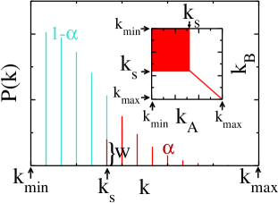
Figure 1: (Color online) Schematic of the degree distribution used to correlate the interdependent networks. If $k_{s}$ is the minimal degree for which the nodes are correlated, $\alpha$ represents the fraction of correlated interdependent nodes denoted by red, and $w$ is the fraction of interdependent correlated nodes with degree $k_{s}$. The light blue region represents the fraction $1-\alpha$ of uncorrelated nodes. In the inset we show with red color the pairs of interdependent nodes with degree $k_{A}-k_{B}$ present in this model.

As $P[k_{A},k_{B}]=P[k_{B},k_{A}]$ and by the symmetry of Eqs. (Triple Point in Correlated Interdependent Networks) and (Triple Point in Correlated Interdependent Networks) in the steady state ($n\to\infty$), $pf_{A\infty}=f_{B\infty}\equiv f_{\infty}$, and the self-consistent equations reduce to

$$f_{\infty}=p\sum_{k_{A}=k_{\rm min}}^{k_{\rm max}}\sum_{k_{B}=k_{\rm min}}^{k_{\rm max}}\frac{k_{B}P[k_{A},k_{B}]}{\langle k\rangle}(1-(1-f_{\infty})^{k_{A}})(1-(1-f_{\infty})^{k_{B}-1}).$$ (11)

We apply this model to pure scale-free (SF) networks with $\lambda=2.5$, $k_{\rm min}=2$ and maximal degree cutoff $k_{\rm max}=N^{1/2}$, with $N=10^{6}$ Boguñá et al. (2004). Here the finite cutoff mimics real networks in which resources and energy are limited and nodes cannot have an unbounded number of links Amaral et al. (2000).

In Fig. 2 we show the solution of the theoretical equations (1)–(Triple Point in Correlated Interdependent Networks) and the simulation results for the size of the GC of network A, $\Psi_{n}$, as a function of the stage number $n$ (Fig. 2a) and $\Psi_{\infty}$ as a function of the $p$ for different values of $\alpha$ (Fig. 2b) .

\begin{overpic}[scale={0.27}]{temp.eps} \put(80.0,30.0){} \end{overpic}

\begin{overpic}[scale={0.27}]{corr.eps} \put(80.0,30.0){} \end{overpic}

Figure 2: (Color online) Cascade of failure on network $A$ for different values of $\alpha$ and $q=1$ on SF networks with $\lambda=2.5$ and $2\leq k\leq 1000$. Figure a: $\Psi_{n}$ for $\alpha=0.01\%$ and $p=0.640$ (green, $\triangle$), $p=0.630$ (black, $\square$) and $p=0.622$ (red, $\bigcirc$) obtained from three single realizations of the simulations (symbols) and from Eqs. (1)-(Triple Point in Correlated Interdependent Networks) (solid line). In the inset we show a log-linear figure of the exponential decay of $\Psi_{n}$ to $\Psi_{\infty}$. The dashed lines correspond to the exponential fit of the theoretical results with a characteristic time $\tau=2.70$, $\tau=4.5$ and $\tau=1.35$ for $p=0.640$, $p=0.630$ and $p=0.622$, from top to bottom. Figure b: $\Psi_{\infty}$ as a function of $p$ obtained from simulations (symbols) and from Eqs. (1)-(Triple Point in Correlated Interdependent Networks) (solid lines) for $\alpha=0.001\%$ (black, $\square$), $\alpha=0.01\%$ (green, $\triangle$), $\alpha=0.1\%$(red, $\bigcirc$). In the inset we plot the main figure in log-linear scale in order to capture the abrupt collapse of the GC as explained in the text. The symbols are the average over 100 network realizations.

The figures show an excellent agreement between the theoretical results and the simulations. In the temporal evolution, Fig. 2a shows that a small variation in $p$ ($\Delta p\approx 0.02$) can dramatically change the final size of the GC. The inset of Fig. 2a shows that the approach of $\Psi_{n}$ to $\Psi_{\infty}$ is exponential. This behavior is due to the fact that the number of iterations of $f_{n}$ in Eqs. (Triple Point in Correlated Interdependent Networks) and (Triple Point in Correlated Interdependent Networks) needed to reach the steady state is the same as the number of iterations needed to find the fixed point of Eq. (11), in which the approach of $\Psi_{n}$ to fixed point $\Psi_{\infty}$ is exponential Buldyrev et al. (2010) and, as a consequence, the temporal percolating dilution slows down. We can also see that at $p\approx 0.63$ the dilution rate decreases more quickly than for other values of $p$, i.e., the size of the functional networks decays slowly, indicating that there is time to intervene and prevent the collapse of the GC. This slow behavior around critical points are shown as peaks in the number of iteration (NOI) steps needed to reach the steady state, as we will show below. Figure 2b shows that, as $\alpha$ increases, the system is still functional for high initial failure values. The critical threshold $p_{c}$ at which the system is completly destroyed decreases and thus the networks are more robust.

\begin{overpic}[scale={0.27}]{noi.eps} \put(80.0,30.0){} \end{overpic}

\begin{overpic}[scale={0.27}]{phase.eps} \put(80.0,30.0){} \end{overpic}

Figure 3: (Color online) Figure (a): the NOI as a function of $p$, obtained from the iterations of Eqs. (1)-(Triple Point in Correlated Interdependent Networks). The network parameters and the color are the same than in Fig. 2. The labels denote the position of the peaks for $\alpha=0.001\%$ (label $1$), $\alpha=0.01\%$ (label $2$), $\alpha=0.1\%$(label $3$). Figure (b): phase diagram in the plane $\alpha-p$: i) the light yellow area corresponds to the nonfunctional phase, $i.e$, $\Psi_{\infty}=\phi_{\infty}=0$, ii) the green area corresponds to a partial functional phase in which the size of the GC of both networks is $\lesssim 10^{-3}$ and iii) the white area corresponds to a functional phase where $\Psi_{\infty}=\phi_{\infty}\gtrsim 10^{-2}$. The black point on the left corresponds to the triple point. The solid lines represent the abrupt change on the network’s sizes and the dotted line, which it is defined for $\alpha>\alpha_{c}$, represents a fast and continuous variation of $\Psi_{\infty}$ at $p_{c}^{+}$.

Note that, because we are using a finite degree cutoff when $\alpha\to 1$, the threshold does not go to zero, but when $k_{\rm max}\to\infty$ in SF networks with $\lambda\leq 3$ and $\alpha=1$, $p_{c}\to 0$ in this limit Buldyrev et al. (2011).

In order to demonstrate how correlation improves the robustness of the networks in Fig. 3a we show the NOI of these systems. For very low values of $\alpha$ there is only one peak at the critical threshold $p_{c}$ that is related to a first order percolating transition. Surprisingly, for increasing $\alpha$ (see the case of $\alpha=0.01\%$ in the figure) there is another peak around the threshold $p_{c}^{+}>p_{c}\equiv p_{c}^{-}$ at which the sizes of the GCs decrease abruptly but, because the hubs support each other, the functional networks are not destroyed, and the robustness of the system against failure cascades is enhanced. For higher values of $\alpha$ we also find that there is a sharp peak that corresponds to a first order phase transition at $p=p_{c}^{-}$ and a rounded peak at $p=p_{c}^{+}$ around which the size of the GC decreases continuously with an increasing value of its derivative with respect to $p$, $d\Psi_{\infty}/dp$ close to $p_{c}^{+}$. These findings suggest that finite correlations generate a crossover between an abrupt and a continuous-sharply decreasing in the sizes of the GCs.

Figure 3b shows the rich phase diagram in the $p-\alpha$ plane. Note that as $\alpha$ increases, the line of the first order transition that separates a funtional GC phase from a nonfunctional phase forks into two branches, generating a new phase characterized by a small GC ($\lesssim 10^{-3}$). Around this point small fluctuations in the temporal evolution—or in the steady state—can induce an abrupt change in the size of the GC, which is reminiscent of the instability of the triple point of liquids where three phases coexist Stanley (1971). The lower branch that emerges from the triple point corresponds to the first order transition that separates functional from nonfunctional phases. The upper one corresponds to the second threshold where the dynamics slows down and, at $\alpha=\alpha_{c}=0.0218\%$ Exx , the transition changes from an abrupt variation to a rapid but continuous variation of $\Psi_{\infty}(p)$. The small value of $\alpha_{c}$ indicates that a small correlation of the highest degree nodes can avoid the abrupt change in the size of the GC. We found the same qualitative behavior for other SF networks with $2<\lambda\leq 3$ , indicating that the triple point is characteristic of nontrivial patterns of interdependency.

In summary, we have used a general framework to describe the temporal behavior of failure cascades with any pattern of interdependency links, and we have found a rich phase diagram for degree-degree correlated interdependency with a triple point at which a first order transition line splits into two first order lines with an abrupt collapse of the sizes of the functional networks. The agreement between theory and simulations is excellent. Our framework can be extended to study the dynamics of failure cascades and the robusteness of networks with degree-degree correlation in their connectivity links and in their multiple interdependent links, where we expect to find a rich phase diagram Valdez et al. (2013).

I acknowledgments

L.D.V, P.A.M and L.A.B thank UNMdP and FONCyT (Pict 0293/2008) for financial support. H.E.S thanks ONR (Grant N00014-09-1-0380, Grant N00014-12-1-0548), DTRA (Grant HDTRA-1-10-1- 0014, Grant HDTRA-1-09-1-0035), and NSF (Grant CMMI 1125290).

References

- Rinaldi et al. (2001) S. M. Rinaldi, J. P. Peerenboom, and T. K. Kelly, Control Systems, IEEE 21, 11 (2001).
- Vespignani (2010) A. Vespignani, Nature 464, 984 (2010).
- Rosato et al. (2008) V. Rosato, L. Issacharoff, F. Tiriticco, S. Meloni, S. Porcellinis, and R. Setola, International Journal of Critical Infrastructures 4, 63 (2008).
- Buldyrev et al. (2010) S. V. Buldyrev, R. Parshani, G. Paul, H. E. Stanley, and S. Havlin, Nature 464, 1025 (2010).
- Buldyrev et al. (2011) S. V. Buldyrev, N. W. Shere, and G. A. Cwilich, Phys. Rev. E 83, 016112 (2011).
- Gao et al. (2012) J. Gao, S. V. Buldyrev, H. E. Stanley, and S. Havlin, Nature Physics 8, 40 (2012).
- Parshani et al. (2010a) R. Parshani, C. Rozenblat, D. Ietri, C. Ducruet, and S. Havlin, EPL 92, 68002 (2010a).
- Hu et al. (2013) Y. Hu, D. Zhou, R. Zhang, Z. Han, C. Rozenblat, and S. Havlin, Phys. Rev. E 88, 052805 (2013).
- Parshani et al. (2010b) R. Parshani, S. V. Buldyrev, and S. Havlin, Phys. Rev. Lett. 105, 048701 (2010b).
- Huang et al. (2011) X. Huang, J. Gao, S. V. Buldyrev, S. Havlin, and H. E. Stanley, Phys. Rev. E 83, 065101 (2011).
- Zhou et al. (2013) D. Zhou, J. Gao, H. E. Stanley, and S. Havlin, Phys. Rev. E 87, 052812 (2013).
- Schneider et al. (2013) C. M. Schneider, N. Yazdani, N. A. Araújo, S. Havlin, and H. J. Herrmann, Scientific Reports 3, 1969 (2013).
- Braunstein et al. (2007) L. A. Braunstein, Z. Wu, Y. Chen, S. V. Buldyrev, T. Kalisky, S. Sreenivasan, R. Cohen, E. López, S. Havlin, and H. E. Stanley, International Journal of Bifurcation and Chaos 17, 2215 (2007).
- Newman et al. (2001) M. E. Newman, S. H. Strogatz, and D. J. Watts, Physical Review E 64, 026118 (2001).
- Callaway et al. (2000) D. S. Callaway, M. E. J. Newman, S. H. Strogatz, and D. J. Watts, Phys. Rev. Lett. 85, 5468 (2000).
- Son et al. (2012) S.-W. Son, G. Bizhani, C. Christensen, P. Grassberger, and M. Paczuski, EPL 97, 16006 (2012).
- Baxter et al. (2012) G. Baxter, S. Dorogovtsev, A. Goltsev, and J. Mendes, Phys. Rev. Lett. 109, 248701 (2012).
- Colizza et al. (2006) V. Colizza, A. Flammini, M. A. Serrano, and A. Vespignani, Nature Physics 2, 110 (2006).
- Xu et al. (2010) X.-K. Xu, J. Zhang, and M. Small, Phys. Rev. E 82, 046117 (2010).
- Boguñá et al. (2004) M. Boguñá, R. Pastor-Satorras, and A. Vespignani, Eur. Phys. J. B 38, 205 (2004).
- Amaral et al. (2000) L. A. N. Amaral, A. Scala, M. Barthélémy, and H. E. Stanley, Proceedings of the National Academy of Sciences 97, 11149 (2000).
- Stanley (1971) H. E. Stanley, Introduction to Phase Transitions and Critical Phenomena (Oxford University Press, 1971).
- (23) In order to calculate the critical point, we solve geometrically the Eq. (11) using the intersection between the identity function and the r.h.s of Eq. (11). A critical point corresponds to the value of at which the angle in the intesection point between the identity function and the r.h.s of Eq. (11) is minimun .
- Valdez et al. (2013) L. Valdez, P. Macri, and L. Braunstein, arXiv preprint arXiv:1310.6345 (2013).