The Effects of Curvature and Expansion on Helium Detonations on White Dwarf Surfaces

Abstract

Accreted helium layers on white dwarfs have been highlighted for many decades as a possible site for a detonation triggered by a thermonuclear runaway. In this paper, we find the minimum helium layer thickness that will sustain a steady laterally propagating detonation and show that it depends on the density and composition of the helium layer, specifically ¹²C and ¹⁶O. Detonations in these thin helium layers have speeds slower than the Chapman-Jouget (CJ) speed from complete helium burning, $v_{CJ}=1.5\times 10^{9}$cm/s. Though gravitationally unbound, the ashes still have unburned helium ($\approx 80\%$ in the thinnest cases) and only reach up to heavy elements such as ⁴⁰Ca, ⁴⁴Ti, ⁴⁸Cr, and ⁵²Fe. It is rare for these thin shells to generate large amounts of ⁵⁶Ni. We also find a new set of solutions that can propagate in even thinner helium layers when ¹⁶O is present at a minimum mass fraction of $\approx 0.07$. Driven by energy release from $\alpha$ captures on ¹⁶O and subsequent elements, these slow detonations only create ashes up to ²⁸Si in the outer detonated He shell. We close by discussing how the unbound helium burning ashes may create faint and fast “.Ia” supernovae as well as events with virtually no radioactivity, and speculate on how the slower helium detonation velocities impact the off-center ignition of a carbon detonation that could cause a Type Ia supernova in the double detonation scenario.

1. Introduction

Recent observations indicating a large population of compact double white dwarf (WD) binaries with one member being a low mass ($M<0.2\ M_{\odot}$) helium WD (Brown et al., 2010; Kilic et al., 2011; Brown et al., 2012; Kilic et al., 2012; Brown et al., 2013), especially those that will merge within a Hubble time, highlight the need for understanding the outcomes of helium accretion in such systems. Previous theoretical work on helium accretion in compact binaries has shown the possibility of the accreted helium layer becoming dynamically unstable (Bildsten et al., 2007) leading to deflagrations or detonations in the accreted layer (Shen & Bildsten, 2009; Shen et al., 2010; Woosley & Kasen, 2011). Such events are predicted to be characteristically ‘fast and faint’ due to their low ejecta mass and partial burning to radioactive isotopes such as ⁵⁶Ni. At the same time, rapidly-evolving transients that stand apart from traditional supernova categories were discovered such as SN 2002bj (Poznanski et al., 2010), SN 2010X (Kasliwal et al., 2010), and SN 2005ek (Drout et al., 2013), while some historic supernovae such as SN 1885A and SN 1939B were recognized as potential members of a class of fast, low ejecta-mass events (Perets et al., 2011).

Nondegenerate helium burning stars may also be relevant donors for peculiar Type Ia explosions. Some of the members of the recently proposed “Type-Iax” supernovae (SNe 2004cs & 2007J) show helium lines in their spectra that may point to helium playing a role in their explosion (Foley et al., 2013), though perhaps through deflagration rather than detonation (Woosley & Kasen, 2011). The discovery of helium burning stars in binaries with WDs that will initiate mass transfer before their helium burning phase ends (Vennes et al., 2012; Geier et al., 2013) widens the spectrum of helium accretion scenarios. This also allows for the possibility of accreting material enriched with helium burning products such as ¹²C and ¹⁶O.

State of the art calculations of helium detonations on WDs include computationally intensive full-star 3D simulations (Moll & Woosley, 2013), models with 1D radially-propagating detonations (Shen et al., 2010; Waldman et al., 2011; Woosley & Kasen, 2011), and level-set methods (Fink et al., 2010; Sim et al., 2012), including detonation-shock-dynamics (Dunkley et al., 2013). Comparison against a 1D model that can be treated with numerical techniques that have explicit error control is an essential verification test of multidimensional models. This allows confidence that the relevant reaction scales are determined independent of resolution limitations. Additionally, the 1D model allows a physical understanding of the mechanism of reaction freeze out. Along with some parameterization of the WD properties, this makes it possible to efficiently survey the expected yields for the full variety of He shell thicknesses, compositions, and densities. Motivated by the stable, laterally propagating helium detonation solutions found in the simulations of Townsley et al. (2012), we investigate the effects of post-shock expansion through both shock-front curvature and radial expansion on a 1D steady-state detonation. In this paper we present criteria for the propagation of a steady detonation wave in a uniform medium that is allowed to expand behind the shock front, and characterize the speeds and burning products of such detonations.

In §2, we outline the standard one-dimensional formalism for determining the post-shock structure of detonations. Section 3 discusses astrophysically motivated helium accretion scenarios and the results of multidimensional detonation simulations we wish to capture in our 1D model, while §4 explains our modifications of the ZND formalism to include the effects of radial expansion and curvature. In §5 we report how these effects modify detonation velocities and nucleosynthesis, and present comparisons to 2D hydrodynamic simulations of detonations in constant-density layers in FLASH. We extend these comparisons to detonations in finite gravity environments and map our results to WD core + envelope configurations in §6 and conclude in §7.

2. Detonations in One Dimension

A detonation consists of a leading shock wave, self-sustained by net exothermic reactions which release a specific energy $\Delta q$ (erg/g) in the shocked material. In contrast to a deflagration, where heat transport by thermal conduction leads to subsonic propagation of the burning, detonations move at supersonic speeds that depend most strongly on $\Delta q$ via $v^{2}_{\rm det}\propto\Delta q$. In this section, we summarize the properties of 1D detonations in plane-parallel geometry and explain why modifications are necessary to model surface detonations on WDs. We first discuss the equations that describe steady detonations in §2.1, followed by detonation velocity determination for 1D plane-parallel detonations in §2.2.

2.1. Zel’dovich-von Neumann-Döring formalism

The one-dimensional model for a steady detonation was developed by Zel’dovich (1940), von Neumann (1942, 1963), and Döring (1943), coupling the hydrodynamic equations to the burning equations under the steady-state assumption in the frame moving with the detonation front. The Zel’dovich-von Neumann-Döring (ZND) model calculates the post-shock structure, and is an excellent starting point for modeling post-shock expansion terms later in this paper. We derive the ZND equations from the hydrodynamic equations in Eulerian coordinates, neglecting viscosity and conduction:

$$\frac{\partial\rho}{\partial t}+{\bf\nabla}\cdot\left(\rho{\bf u}\right) =0,$$ (1)

$$\frac{\partial{\bf u}}{\partial t}+({\bf u}\cdot{\bf\nabla}){\bf u}+\frac{1}{\rho}{\bf\nabla}P-\frac{{\bf F_{\rm ext}}}{\rho} =0,$$ (2)

$$\frac{\partial}{\partial t}\left(\rho e\right)+{\bf\nabla}\cdot\left[(\rho e+P){\bf u}\right]-\rho\epsilon =0,.$$ (3)

Here, $\rho(t,{\bf x})$ is the density of the fluid, ${\bf u}(t,{\bf x})$ is the (Eulerian) velocity, $P(t,{\bf x})$ is the pressure, ${\bf F_{\rm ext}}(t,{\bf x})$ are any external forces on the fluid (e.g. gravity), $e(t,{\bf x})$ is the internal specific energy including the nuclear binding energy (in erg/g), and $\epsilon(t,{\bf x})$ is the local heating/cooling function (in erg g^-1 s^-1). These equations simplify under the assumptions used in the ZND formalism. For steady one-dimensional flow, we move into the shock frame ($x$ is now the distance behind the shock front) and write ${\bf u}=u\hat{x}$, ignore terms with $\partial/\partial t$, and set ${\bf F_{\rm ext}}=0$. The energy generation rate $\epsilon$ comes from the release of nuclear binding energy $\Delta q$, where the total nuclear binding energy is

$$q=N_{A}\sum_{i}Q_{i}Y_{i}.$$ (4)

Here, $N_{A}$ is Avogadro’s number, $Q_{i}$ is the nuclear binding energy of the $i^{th}$ species $(Q_{i}>0)$, and $Y_{i}$ is the molar mass fraction, $Y_{i}=X_{i}/A_{i}$, with the mass fraction and atomic weight of the $i^{th}$ species being $X_{i}$ and $A_{i}$, respectively. Since there are no neutrino losses, the energy generation rate is thus

$$\epsilon=\dot{q} =\frac{\partial q}{\partial t}+({\bf u}\cdot{\bf\nabla})q=u\frac{dq}{dx},$$ (5)

where

$$\frac{dq}{dx}=N_{A}\sum_{i}Q_{i}\frac{dY_{i}}{dx},$$ (6)

so that the energy release of a fluid element throughout the detonation,

$$\Delta q=\int\epsilon\ dt=\int\frac{dq}{dx}dx,$$ (7)

can be calculated.

This leaves a concise set of equations describing one-dimensional reactive flow (Fickett & Davis, 1979) :

$$\frac{d}{dx}\left(\rho u\right) = 0,$$ (8)

$$\frac{d}{dx}\left(P+\rho u^{2}\right) = 0,$$ (9)

$$\frac{d}{dx}\left((e-q)+\frac{P}{\rho}+\frac{u^{2}}{2}\right) = 0,$$ (10)

$$\frac{d}{dx}\left(X_{i}\right) = \frac{R_{i}(\rho,T,\bf{X})}{u}.$$ (11)

Equations (8)-(10) express mass, momentum, and energy conservation, while equation (11) evolves the composition due to nuclear burning. The reaction rates $R_{i}$ are taken from MESA’s net module (Paxton et al., 2011, 2013), using data from NACRE and JINA Reaclib (Rauscher & Thielemann, 2000; Cyburt et al., 2010).

In order to compare to other derivations, we take $\rho,T,u,{\bf X}$ as the independent variables for our ZND calculation, where ${\bf X}$ is the vector of mass fractions of all isotopes in the reaction network. Using the transformations

$$\frac{dP}{dx} = \left(\frac{\partial P}{\partial\rho}\right)_{{\bf X},T}\frac{d\rho}{dx}+\left(\frac{\partial P}{\partial T}\right)_{{\bf X},\rho}\frac{dT}{dx}$$ (12)

$$+ \sum_{i}\left(\frac{\partial P}{\partial X_{i}}\right)_{X_{j},\rho,T}\frac{dX_{i}}{dx},$$

$$\frac{de}{dx} = \left(\frac{\partial e}{\partial\rho}\right)_{{\bf X},T}\frac{d\rho}{dx}+\left(\frac{\partial e}{\partial T}\right)_{{\bf X},\rho}\frac{dT}{dx}$$ (13)

$$+ \sum_{i}\left(\frac{\partial e}{\partial X_{i}}\right)_{X_{j},\rho,T}\frac{dX_{i}}{dx},$$

we derive evolution equations for $\rho,T$, and $u$ as a function of position behind the shock front. Henceforth, partial derivatives are assumed to hold all variables in the $\{\rho,T,{\bf X}\}$ set constant except the one(s) being differentiated by unless otherwise noted. In this case, equations (8)-(11) become

$$\frac{d\rho}{dx} = \frac{1}{c_{s}^{2}-u^{2}}\sum_{i}\frac{dX_{i}}{dx}\left[\left(\frac{\partial P}{\partial e}\right)_{\rho}\left(\frac{\partial e}{\partial X_{i}}\right)-\left(\frac{\partial P}{\partial X_{i}}\right)\right]$$ (14)

$$= -\frac{\rho c_{s}^{2}\sigma_{i}R_{i}}{u(c_{s}^{2}-u^{2})},$$

$$\frac{dT}{dx} = \left(\frac{\partial P}{\partial T}\right)^{-1}\left[\frac{d\rho}{dx}\left(u^{2}-\left(\frac{\partial P}{\partial\rho}\right)\right)-\sum_{i}\left(\frac{\partial P}{\partial X_{i}}\right)\frac{dX_{i}}{dx}\right],$$ (15)

$$\frac{du}{dx} = -\frac{u}{\rho}\frac{d\rho}{dx},$$ (16)

$$\frac{dX_{i}}{dx} = \frac{R_{i}(\rho,T,\bf{X})}{u}.$$ (17)

where

$$c_{s}^{2}=\left(\frac{\partial P}{\partial\rho}\right)_{{\bf X},S}=\left(\frac{\partial P}{\partial\rho}\right)+\left(\frac{\partial P}{\partial e}\right)_{\rho}\left(\frac{P}{\rho^{2}}-\left(\frac{\partial e}{\partial\rho}\right)\right),$$ (18)

evaluated at fixed entropy, $S$, and composition, is the frozen sound speed, and consistent with the detonation literature (Fickett & Davis, 1979; Sharpe, 1999), the thermicity, $\sum_{i}\sigma_{i}R_{i}$, is defined as the rate of conversion of nuclear energy into thermal energy, where

$$\sigma_{i}=\frac{1}{\rho c_{s}^{2}}\left[\left(\frac{\partial P}{\partial Y_{i}}\right)-\left(\frac{\partial e}{\partial Y_{i}}\right)\left(\frac{\partial P}{\partial T}\right)\right],$$ (19)

and the equation governing reaction rates remains equation (11).

Numerical integration of equations (14) - (17) can be made far more efficient if we have analytic expressions for their derivatives with respect to each of the independent variables, i.e. the Jacobian terms. In order to compute these, we rewrite the compositional derivatives in terms of the independent variables that the MESA equation of state (EOS) uses, $\{\rho,T,\bar{A},\bar{Z}\}$, where $\bar{A}$ is the mean atomic weight of the mixture,

$$\bar{A}=\frac{\sum_{i}n_{i}A_{i}}{\sum_{i}n_{i}},$$ (20)

and $\bar{Z}$ is the mean charge of the mixture,

$$\bar{Z}=\frac{\sum_{i}n_{i}Z_{i}}{\sum_{i}n_{i}},$$ (21)

where $n_{i}=\rho N_{A}Y_{i}$ is the particle density of the $i^{th}$ species and $Z_{i}$ the respective charge. The ZND equations, (14) - (17), are then rewritten with $\partial/\partial X_{i}$ in terms of $\partial/\partial\bar{A}$ and $\partial/\partial\bar{Z}$. The appropriate transformations are

$$\left(\frac{\partial}{\partial X_{i}}\right)_{X_{j}}=\left(\frac{\partial\bar{A}}{\partial X_{i}}\right)_{X_{j}}\left(\frac{\partial}{\partial\bar{A}}\right)_{\bar{Z}}+\left(\frac{\partial\bar{Z}}{\partial X_{i}}\right)_{X_{j}}\left(\frac{\partial}{\partial\bar{Z}}\right)_{\bar{A}},$$ (22)

where

$$\left(\frac{\partial\bar{A}}{\partial X_{i}}\right)_{X_{j}} =\frac{\bar{A}(A_{i}-\bar{A})}{A_{i}}$$ (23)

$$\left(\frac{\partial\bar{Z}}{\partial X_{i}}\right)_{X_{j}} =\frac{\bar{A}(Z_{i}-\bar{Z})}{A_{i}}.$$ (24)

Thus, for example

$$\left(\frac{\partial P}{\partial X_{i}}\right)_{X_{j}}=\frac{\bar{A}(A_{i}-\bar{A})}{A_{i}}\left(\frac{\partial P}{\partial\bar{A}}\right)_{\bar{Z}}+\frac{\bar{A}(Z_{i}-\bar{Z})}{A_{i}}\left(\frac{\partial P}{\partial\bar{Z}}\right)_{\bar{A}}.$$ (25)

These relations will be used in constructing the Jacobian for the ZND equations presented here, and beyond as we explore modifications to the ZND equations.

2.2. Chapman-Jouget Detonations

A Chapman-Jouget (CJ) detonation is one in which the burning ceases (due to exhaustion of fuel) when the post-shock flow becomes sonic relative to the shock front (Fickett & Davis, 1979). Physically, this means that all the nuclear energy released can be used to propagate the detonation front, since the entire reaction zone is in sonic contact with it. Such a detonation occurs at a unique velocity, given the initial conditions ($\rho_{0}$, $T_{0}$, ${\bf X}_{0}$). The CJ velocity for helium detonations has a weak dependence on initial density (Timmes & Niemeyer, 2000), and is $v_{\rm CJ}=1.52\times 10^{9}$ cm/s at an initial density of $\rho_{0}=5\times 10^{5}$ g/cm³. Calculating this velocity requires a knowledge of the final state of the ashes, and in general requires a calculation of nuclear statistical equilibrium (NSE) near the end of the reaction zone. At these low densities, the final state is virtually pure ⁵⁶Ni, while at higher densities $(\rho_{0}\gtrsim 10^{6}$ g/cm${}^{3})$ the high post-shock temperatures can lead to photo-disintegration and electron capture, which significantly alters the final state. In order to avoid a lengthy digression on the final states of CJ detonations in pure helium at high densities, we employ a simple 13-isotope alpha chain for our CJ calculations here (Timmes, 1999). In a $\gamma$-law equation of state, $P=(\gamma-1)\rho e$, the detonation velocity is related to the post-shock energy release $\Delta q$ as (Fickett & Davis, 1979)

$$v_{\rm det}^{2}=2\left(\gamma^{2}-1\right)\Delta q.$$ (26)

Although our equation of state is more detailed, the requirement that the burning used to propel the detonation remains in sonic contact with the shock front guides us to expect the scaling $v_{\rm det}^{2}\propto\Delta q$ in general.

We first calculate $v_{\rm CJ}$ via the standard Hugoniot construction (see Fickett & Davis (1979)) assuming a final state of pure ⁵⁶Ni and then use the post-shock conditions immediately behind the shock front to start integrating the ZND equations (14) - (17). We integrate the reaction network using a stiff ODE integrator - a linearly implicit Runge-Kutta method included with MESA (Lang & Verwer, 2001). Since determination of $v_{\rm CJ}$ is independent of the reaction network used in integrating the ZND equations, the resultant nucleosynthesis may differ from the assumed final state in the CJ calculation. We therefore check the final NSE state and iterate this procedure - choosing a new smaller value for $v_{\rm CJ}$ and thus a slightly less fully burned CJ state if the NSE state corresponds to a smaller $\Delta q$ than was assumed, otherwise choosing a larger value for $v_{\rm CJ}$ - until the composition used in the CJ state conforms to the NSE state found by network integration.

We show a spatial profile of the thermodynamic variables and composition in the shock frame in Figures 1 - 3 for CJ detonations in pure helium at initial densities of $\rho_{0}=5\times 10^{5}$ g/cm³ and $\rho_{0}=2\times 10^{6}$ g/cm³, respectively. The detonation with $\rho_{0}=5\times 10^{5}$ g/cm³ burns almost completely to ⁵⁶Ni, while the detonation with $\rho_{0}=2\times 10^{6}$ g/cm³ shows signs of photo-disintegration at late times. Low-density CJ detonations in pure helium take a very long distance to achieve near-total energy release, typically much larger than the circumference of a C/O WD as shown in Figure 4. Formally the material will never become fully burned, so length scales of ever increasing energy release percentage will grow until NSE is achieved.

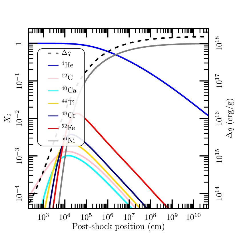
Figure 1.— Nucleosynthesis profile of a CJ detonation in pure helium with $\rho_{0}=5\times 10^{5}$ g/cm³, $T_{0}=10^{8}$ K. The detonation velocity is $v_{\rm CJ}=1.523\times 10^{9}$ cm/s. Solid lines are nuclear abundances and correspond to the left axis, while the dashed line is the cumulative energy release - corresponding to the right axis. It takes a distance of $1.8\times 10^{9}$ cm to achieve $95\%$ of the total energy release.

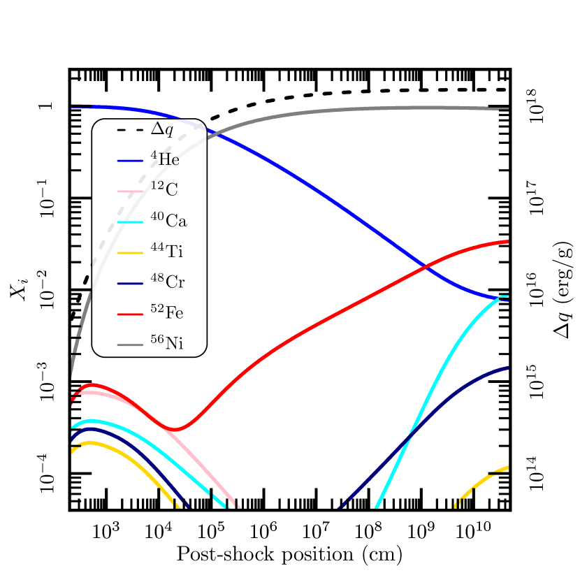
Figure 2.— Nucleosynthesis profile of a CJ detonation in pure helium with $\rho_{0}=2\times 10^{6}$ g/cm³, $T_{0}=10^{8}$ K. The detonation velocity is $v_{\rm CJ}=1.566\times 10^{9}$ cm/s. Solid lines are nuclear abundances and correspond to the left axis, while the dashed line is the cumulative energy release - corresponding to the right axis. It takes a distance of $6.3\times 10^{7}$ cm to achieve $95\%$ of the total energy release.

Figure 3.— Thermodynamic profile of CJ detonations in pure helium with the same starting conditions as Figures 1 ($\rho_{0}=5\times 10^{5}$ g/cm³ - solid lines) and 2 ($\rho_{0}=2\times 10^{6}$ g/cm³ - dashed lines).

A comparison that highlights when the finite thickness of a helium layer will affect the burning is the ratio of scale height to the burning length. We define a measure of the energy release length scale, $l_{95}$, as the distance behind the shock front (in the shock frame) where $95\%$ of the total energy is released. We compare this to the pressure scale height on a star, $H_{s}=P_{0}/(\rho_{0}g)$, as a function of ambient density $\rho_{0}$ in Figure 4 (cf. Timmes & Niemeyer (2000)). For lower densities, $l_{95}$ is much larger than $H_{s}$, while at higher initial densities, the energy release length scale is much smaller than the scale height of the helium layer. We therefore expect the finite thickness of the helium layer to have the largest impact on nucleosynthesis for the thinner cases with lower base densities. A complete burn to ⁵⁶Ni is not possible for a laterally propagating detonation on the surface of a WD. Low-density detonations do not have enough space to burn to completion, while high-density cases experience significant photo-disintegration of synthesized isotopes.

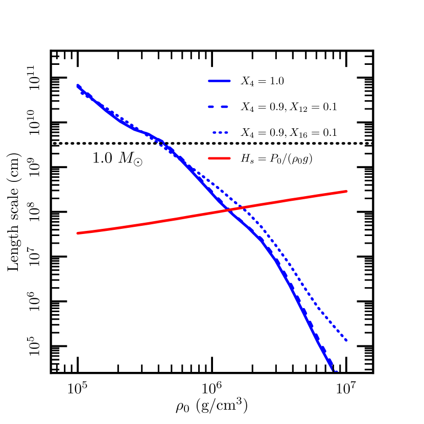
Figure 4.— Length scales to release $95\%$ of the total energy, $l_{95}$, as a function of initial density for helium layers with initial ¹²C and ¹⁶O mass fractions and $T_{0}=10^{8}$ K (blue lines). The scale height of the atmosphere (red line) is computed using $g=3\times 10^{8}$ cm/s² and is smaller than $l_{95}$ for lower initial densities, showing that complete burning and CJ detonations are not formally possible in such envelopes, while higher-density envelopes will be affected less by the finite scale height of the material. The horizontal black dotted line shows the circumference of a $1.0\ M_{\odot}$ WD with core temperature $10^{7}$ K.

Understanding what happens to the CJ detonation velocity when post-shock energy losses due to curvature and radial expansion occur requires understanding what happens in the post-shock flow at detonation velocities near the CJ velocity. In the absence of endothermic reactions in a simple alpha chain nuclear network, the CJ velocity is the unique velocity at which a freely propagating planar detonation will travel. However, we can integrate the ZND equations with any detonation velocity that we choose. If we pick $v_{\rm det}<v_{\rm CJ}$, then the integration encounters a singularity (the sonic point) when the post-shock flow relative to the shock front reaches the local frozen sound speed, $c_{s}^{2}=(\partial P/\partial\rho)_{{\bf X},S}$ - see equation (14). These detonations are referred to as underdriven detonations, and numerical hydrodynamic simulations show that such planar detonations in helium will strengthen to propagate at $v_{\rm CJ}$, given enough time (Townsley et al., 2012). If we use $v_{\rm det}>v_{\rm CJ}$ then the integration will not hit a singularity, but a supporting pressure is required to sustain such a detonation, called an overdriven detonation. In the absence of such a sustaining pressure (eg. via a piston in a shock tube), this type of detonation will weaken until it propagates at $v_{\rm CJ}$. Figure 5 shows the evolution of the thermodynamic variables behind the shock front for a CJ detonation in pure helium, as well as an overdriven case at a $10\%$ higher detonation velocity, and an underdriven case at $10\%$ lower detonation velocity. Intuition about what happens in planar detonations for velocities near $v_{\rm CJ}$ will guide our analysis of detonation velocities when we include the effects of curvature and expansion.

Figure 5.— Thermodynamic profile of detonations in pure helium with the same starting conditions as Figure 1 - $\rho_{0}=5\times 10^{5}$ g/cm³. The line types correspond to the velocity used to integrate the ZND equations: $v_{\rm det}=v_{\rm CJ}$ (solid lines), $v_{\rm det}=1.1\ v_{\rm CJ}$ (dashed lines), and $v_{\rm det}=0.9\ v_{\rm CJ}$ (dotted lines). The CJ detonation velocity is $v_{\rm CJ}=1.523\times 10^{9}$ cm/s. As discussed in the text, only the detonation with $v_{\rm det}<v_{\rm CJ}$ hits the sonic point, which occurs at $\approx 10^{8}$ cm behind the shock front.

3. Simulations of Detonations in Single Hydrostatic Helium Layers

Here we present the astrophysically-motivated configurations and detonation structures for which, in the following section, we will develop methods for directly computing the basic detonation properties via a ZND-like formalism. A WD with a thin ($\sim$few$\times 10^{-2}M_{\odot}$) He shell undergoing a thermonuclear shell flash is the environment we will study for the propagation of a lateral detonation. Since we will develop ZND-like steady-state calculations of this detonation structure, we utilize a plane parallel calculation under constant (spatially uniform) gravity rather than working in a full star. This is as done in Townsley et al. (2012), and allows us to propagate a detonation into steady state for a given helium layer. We make the further simplification that there is only a $10^{8}$ K He layer, no hot overlying convective zone as was used in Townsley et al. (2012). This isolates expansive characteristics of a single layer and facilitates more direct comparison with our ZND-like calculations.

The computational setup used here is otherwise the same as that used in Townsley et al. (2012). All physics is included in the public FLASH 4 code release, and the Simulation Units, which define the initial condition and mesh refinement, for this and the strip detonation configuration described below are available for download via the web . While for high densities and thick layers NSE will be reached, requiring careful treatment of the coupling between energy release and hydrodynamics, we limit our hydrodynamic cases to those that do not burn to completion, having peak temperatures around 2-3$\times 10^{9}$ K. The hydrodynamic step is taken as 0.8 of the CFL, and the nuclear reactions are substep-integrated assuming constant temperature in the usual operator-split fashion used in the FLASH code. With the low peak temperatures, this is numerically stable. Nuclear reactions are suppressed in the vicinity of shocks, since the computations presented here are not over-resolved. Even so, we see, given sufficient resolution, minimal resolution dependence for integrated quantities like yields, energy release, and detonation speed. The small-scale cellular structure near the detonation front does vary with resolution, in a way similar to that seen for resolved detonations with reactions suppressed in shocks (Papathedore, T. & Messer, B., 2013). However, the effect on the burning products well behind the detonation front appear to be mild. The lower boundary of the hydrostatic layer is treated as discussed in Zingale et al. (2002), with local hydrostatic gradient and a reflecting velocity, as implemented in FLASH 4. The top boundary, located at $8.5\times 10^{8}$ cm above the base of the He layer, is zero-gradient outflow, and the side boundaries near the ignition and at the far end of the domain, where the detonation does not reach in the time of the simulation, are reflecting.

A higher gravity will lead to a geometrically thinner shell for the same base pressure (base density). We expect that the vertical expansion of this shell, i.e. blowout, will have a more significant effect on this thinner shell, causing differences in detonation speed and products despite the fuel density being the same. Figure 6 shows the steady-state temperature and density structure of detonations propagating in helium layers at two different gravities, $g_{8}=2$ (left) and $4$ (right), where $g_{8}$ is gravity in units of $10^{8}$ cm s^-2. The density at the base of the He layer is $5\times 10^{5}$ g cm^-3 in both cases, giving scale heights $H_{s}=P_{0}/\rho_{0}g$ of 1 and 0.5$\times 10^{8}$ cm respectively. The surface of the star is located at a height of approximately 2.5 and 1.2$\times 10^{8}$ cm respectively. The steady-state detonation speeds obtained for these two cases are 0.98 and 0.89$\times 10^{9}$ cm s^-1 respectively. The more prompt lateral expansion of the thinner layer leads to the burning being truncated sooner and a lower propagation speed of the detonation front. These simulations were performed at a resolution of 1km, and the detonation speed varies less than 2% for a factor of 4 coarser resolution. Throughout work in this paper, resolution was adjusted to achieve this level of consistency.

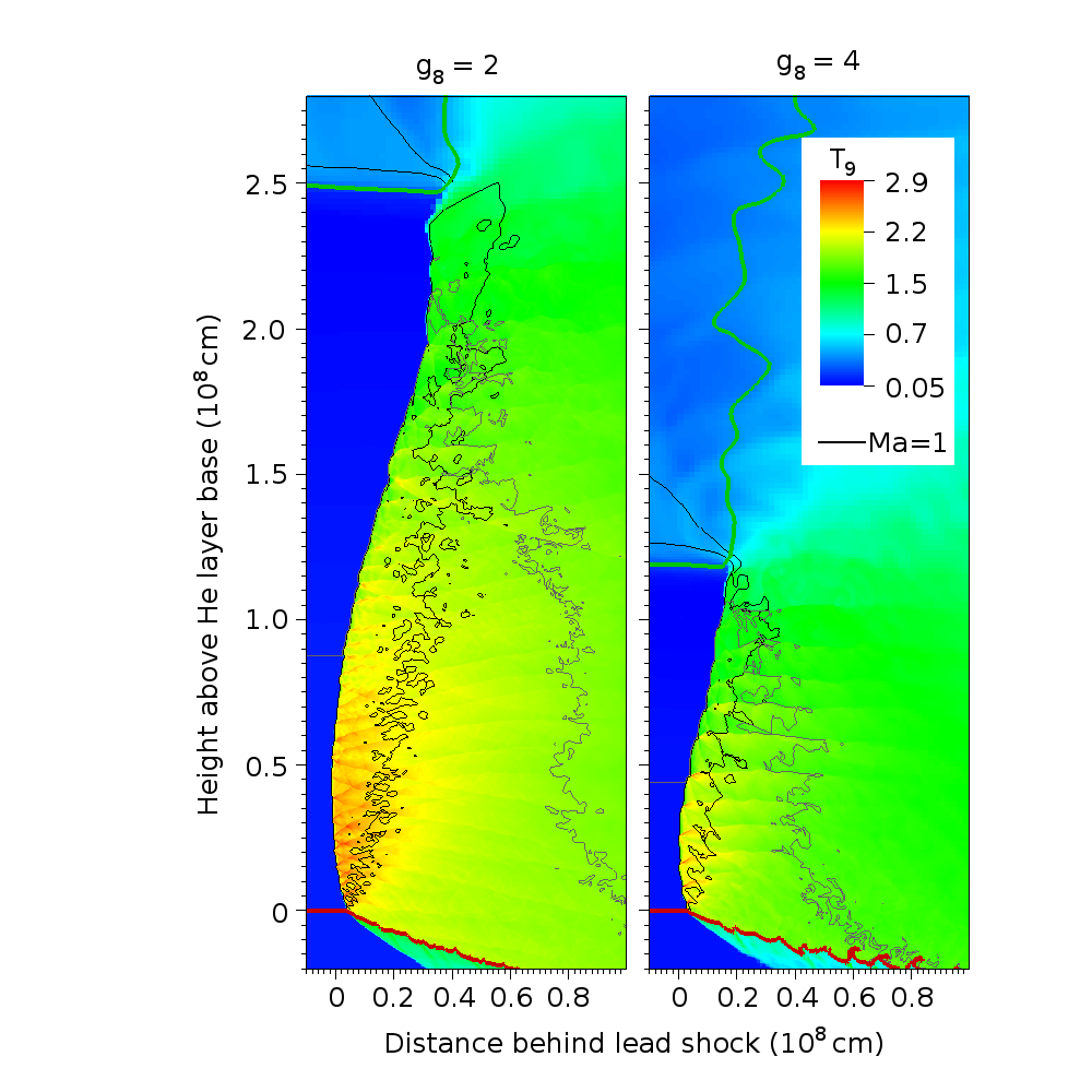
Figure 6.— Steady-state detonation structures in cold helium layers, $T=10^{8}$ K, under two different gravities, $g_{8}=2$ (left) and $4$ (right), in units of $10^{8}$ cm s^-2. Both calculations are performed in plane parallel geometry with constant gravity. The detonation is propagating to the left. Material within sonic contact of the shock front is bounded by the black contour. Specifically, it indicates the sonic locus, the location that the post-shock flow becomes supersonic with respect to the shock front. The thick green contour shows a density of $10^{4}$ g cm^-3, near the surface of the star prior to blowout. The grey contour is at $\rho_{5}=2.5$, half the density at the base of the He layer. The red contour shows the division between the He layer and the underlying core material.

An important contrast created by the difference in shell thickness is the width of the subsonic region behind the shock front. In the shock frame, material entering from the left at the detonation speed, $v_{\rm det}$, is slowed to subsonic speeds (and compressed) by the shock and then accelerated to the right by expansion driven by energy release. This is the driving region for the propagating detonation and, as will be seen below, nearly all the reaction and energy release occurs in this zone. In Figure 6 this region is indicated by the sonic locus in the shock-attached frame, i.e. the Mach number $=1$ contour shown as a thin black line. While the cellular structure of the detonation makes the sonic locus fairly irregular on scales of around $10^{7}$ cm, its average position is stable as the detonation propagates. The distance between the shock and the sonic locus is smaller near the base of the He layer, and the sonic locus in fact meets the shock front at the bottom edge of the He layer. This is due to the rarefaction wave in the fuel layer arising from the interaction with the inert underlying layer as the shock crossing the shell-core boundary locally continues into the interior of the WD rather than being reflected.This corresponds to the low-impedance case shown in Figure 7.26(a) in Bdzil & Stewart (2012). The behavior of the extent of the subsonic region with increasing height is more subtle but qualitatively similar. At lower densities, a propagating detonation will have a larger subsonic region and longer burning time. However after a maximum width at around one scale height above the base of the helium layer, the sonic region becomes slowly smaller, closing with the shock front in a somewhat less clean way near the surface of the star. The decrease in the peak temperature of the burning with height is also evident.

Comparing the two gravities shown in Figure 6, we find that the subsonic region is larger at the lower gravity with the thicker shell. At $g_{8}=2$ it spans $\approx 0.2\times 10^{8}$ cm at its thickest in the central reaction region (height of about $0.5\times 10^{8}$ cm), while at $g_{8}=4$, the subsonic region spans $\approx 0.11\times 10^{8}$ cm. The curvature of the detonation front also shows variation, with the detonation in higher gravity exhibiting a more curved front. As we show in the next sections, this is consistent with truncation of the detonation structure by the upward expansion of the shell transverse to the direction of propagation. In this case the expansion is vertical behind the shock front due to the boundaries above and below. In both cases it appears that the entire shell is in the region affected by the rarefaction originating from the boundary. From the ZND analysis in the previous section (structure shown in Figure 1), $>1$% He by mass remains out to distances as large as $10^{10}$ cm, the 50% reacted length is $\approx 2\times 10^{6}$cm. As a result the burning is quite incomplete on the reaction widths $\sim 10^{7}$ cm observed here.

Even this simplified configuration of a single helium layer in plane parallel presents challenges for comparison to a direct computation of the steady-state structure. The two most significant difficulties are the stratification of the envelope, i.e. the variation of density across the shock front, and the interaction with the mildly-reactive underlying layer, where any minor (numerical) mixing leads to a small amount of extra $\alpha$-capture. This interaction at the shell-core boundary also makes the detonation cells more prominent For these reasons, in sections below we will resort to an even more simplified configuration in which a uniform density strip of He is confined by a low-density non-reactive gas. This configuration is shown in Figure 7. The strip is confined in pressure equilibrium by a hot field of Ni gas with a density of $100$ g cm^-3. In this geometry, the detonation shock will also be curved, with a radius of $R_{c}$, denoted in Figure 7. The curvature is mostly determined by the shock interaction with the edge of the fuel strip (Bdzil & Stewart, 2012). This further simplified geometry is comparable to that in the star, but has the added advantage of symmetric expansion and a uniform fuel density. There are still rarefaction waves entering the helium strip from above and below. In the next section we will develop a direct computation to be compared to the properties of the detonation along the center line of this strip configuration.

Figure 7.— Configuration for uniform-density strip detonation in 2 spatial dimensions. The strip is confined in pressure equilibrium by a hot, low-density gas of Ni, to minimize reactivity.

Figure 8 shows an example of a detonation propagating in the strip geometry with a fuel density of $\rho_{0}=5\times 10^{5}$ g cm^-3 and a lateral strip half-width of $0.25\times 10^{8}$ cm, half the scale height of the $g_{8}=4$ case shown in Figure 6. The structure shown is in steady-state according to a measurement of shock position as a function of time, which gives a very stable speed. It has propagated for 1.0 s since ignition, covering nearly $10^{9}$ cm. The detonation was initiated by setting a high initial temperature, typically $T_{9}=3$, in a circular region the same diameter as the full width of the strip. This initially leads to an overdriven detonation that then weakens to the steady-state self-propagating state as the initial extra pressure support behind is lost to lateral expansion. This simulation is performed with a resolution of $3\times 10^{6}$ cm. The detonation speed the same to within less than $1$% compared to a factor of 2 coarser resolution of $6\times 10^{6}$ cm, and spatial features are very similar at the two resolutions. More features of this calculation will be discussed in later sections.

A critical similarity with the stratified atmosphere is the non-uniform width of the subsonic region due to the expansion from the unconfined edge. This demonstrates that this feature is not related to the density stratification. The distance from the shock to the average sonic locus is also not uniform for any region across the detonation front. This is in contrast to cases shown in Bdzil & Stewart (2012) in which the reaction length scale is much less than the lateral width of the strip of fuel. In the limit of a short reaction length, the shock front can still be curved in much the same way, but away from the edge of the strip, near the centerline, the sonic locus is parallel to the shock. In our case the slowness of the late-time He consumption causes the driving region to extend until it is quenched by the blowout, which depends on the distance from the edge all the way to the centerline. That is, the entire detonation front is in the edge boundary region.

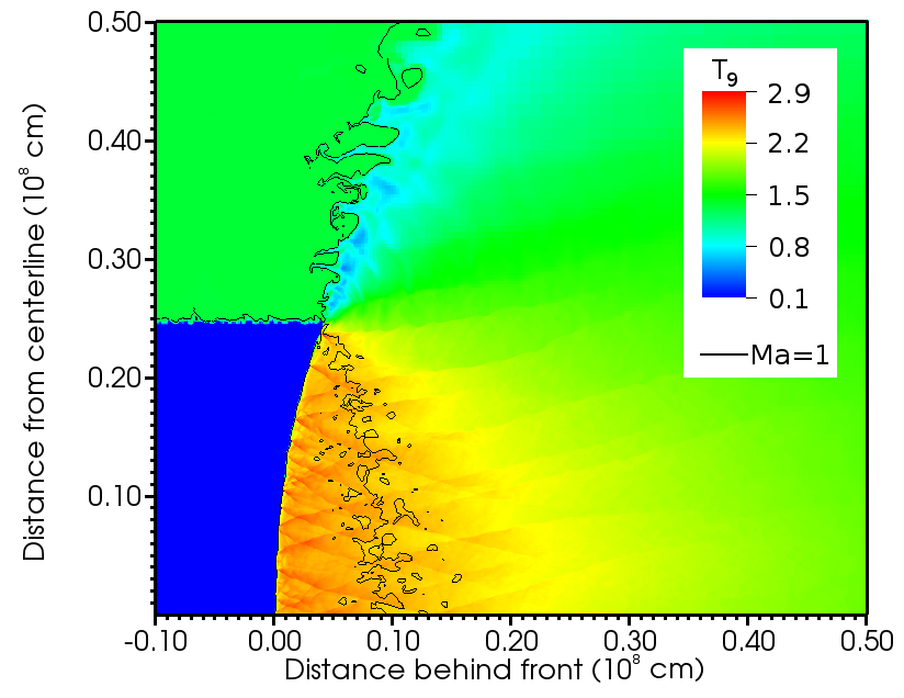
Figure 8.— Temperature distribution of a detonation propagating through a strip of helium at a uniform density of $5\times 10^{5}$ g cm^-3. The helium extends up to a half-width of $0.25\times 10^{8}$ cm. The detonation was ignited far to the right and at the time shown, $1.0$ s, has propagated nearly $10^{9}$ cm. A black countour at Mach number of 1 indicates the sonic locus, the boundary of the subsonic region behind the shock front. The extent of the subsonic region shows no region of uniform distance behind the front, and therefore is clearly everywhere effected by the proximity of the blowout at the edge of the strip.

4. Generalized ZND formalism

Surface detonations in accreted layers on WDs are inherently multidimensional, and the standard ZND equations do not capture important effects such as the post-shock radial expansion or the curved detonation front. These effects have a dramatic impact on the total energy released in a detonation, and thus its propagation speed and burning products.

The modifications to the hydrodynamic equations that simulate post-shock expansion, either due to the curvature of the detonation front or radial expansion, can be written in the form of source terms in the standard 1D hydrodynamic equations (8) - (10):

$$\frac{d}{dx}\left(\rho u_{x}\right) =f_{1},$$ (27)

$$\frac{d}{dx}\left(P+\rho u_{x}^{2}\right) =f_{2},$$ (28)

$$\frac{d}{dx}\left(e+\frac{P}{\rho}+\frac{u_{x}^{2}}{2}\right) =f_{3}.$$ (29)

The standard ZND equations have $f_{1-3}=0$, whereas here they can be arbitrary functions. Deriving the ZND equations from equations (27)-(29) and (11) is straightforward, following the derivation of the standard ZND equations - (14)-(16), we obtain

$$\frac{d\rho}{dx} =\frac{1}{c_{s}^{2}-u_{x}^{2}}\left(\sum_{i}\frac{dX_{i}}{dx}\left[\left(\frac{\partial P}{\partial e}\right)_{\rho}\left(\frac{\partial E}{\partial X_{i}}\right)-\left(\frac{\partial P}{\partial X_{i}}\right)\right]\right.$$

$$+\left.f_{2}-2u_{x}f_{1}-\left(\frac{\partial P}{\partial e}\right)_{\rho}\left[f_{3}-\frac{f_{2}}{\rho}+\frac{u_{x}f_{1}}{\rho}\right]\right),$$ (30)

$$\frac{dT}{dx} =\left(\frac{\partial P}{\partial T}\right)^{-1}\left[\frac{d\rho}{dx}\left(u_{x}^{2}-\left(\frac{\partial P}{\partial\rho}\right)\right)\right.$$

$$-\left.\sum_{i}\left(\frac{\partial P}{\partial X_{i}}\right)\frac{dX_{i}}{dx}+f_{2}-2u_{x}f_{1}\right],$$ (31)

$$\frac{du_{x}}{dx} =\frac{f_{1}}{\rho}-\frac{u_{x}}{\rho}\frac{d\rho}{dx}.$$ (32)

These equations, along with equation (17), govern the post-shock structure of steady, one-dimensional detonation waves with arbitrary source terms in the hydrodynamic equations. We use them here to examine expansive effects (now through radial expansion and curvature) on the detonation, but they are quite general at this point. We derive specific expressions for $f_{1-3}$ due to curvature and expansion in sections A and B of the appendix.

4.1. Determining the detonation velocity from initial geometry

The standard ZND equations (14)-(16), along with our generalized ZND equations (30)-(32), encounter a singularity if the flow in the shock frame becomes sonic ($u_{x}=c_{s}$) - called the sonic point. Recall from section 2.2 that the CJ detonation velocity separated solutions that hit the sonic point ($v_{\rm det}<v_{\rm CJ}$) from solutions that did not hit a sonic point ($v_{\rm det}>v_{\rm CJ}$). In a detonation at $v_{\rm det}=v_{\rm CJ}$ the sonic point appears when burning is complete, but this may formally take infinite length and time to achieve depending on the reaction network used. When we find the CJ velocity using the generalized ZND equations (30)-(32) with blowout and/or curvature effects, we find that the velocity that separates solutions that encounter the sonic point from those that do not is always less than the $v_{\rm CJ}$ we found without source terms. For example, in the case without source terms shown in Figure 1, the separating velocity is $v_{\rm CJ}=1.52\times 10^{9}$ cm/s, whereas for $H=R_{c}/3=5\times 10^{7}$ cm we get a separating velocity of $1.08\times 10^{9}$ cm/s (the relation $R_{c}=3H$ used here will be discussed in Section 5 when comparing to simulations). This general effect on detonation velocity is apparent in Figure 9 which shows the separation between underdriven and overdriven solutions in cases with and without source terms. Similar to He & Clavin (1994), we refer to this CJ-like velocity when source terms are included as the generalized CJ velocity, $v_{\rm gcj}$. While the underdriven solution is unphysical because of the singularity, the overdriven detonation requires a supporting pressure in the following flow, and thus a small $u_{x}$ at large distance. The unsupported, freely propagating solution can be obtained by integrating through the point where both the numerator and denominator in equation (30) are simultaneously zero, thus avoiding the singularity and giving a consistent solution that is sonically disconnected from the following flow. This can only occur at $v_{\rm gcj}$, also called the eigenvalue detonation speed (Fickett & Davis, 1979), and gives a following flow in which the pressure and temperature monotonically fall to cessation of burning.

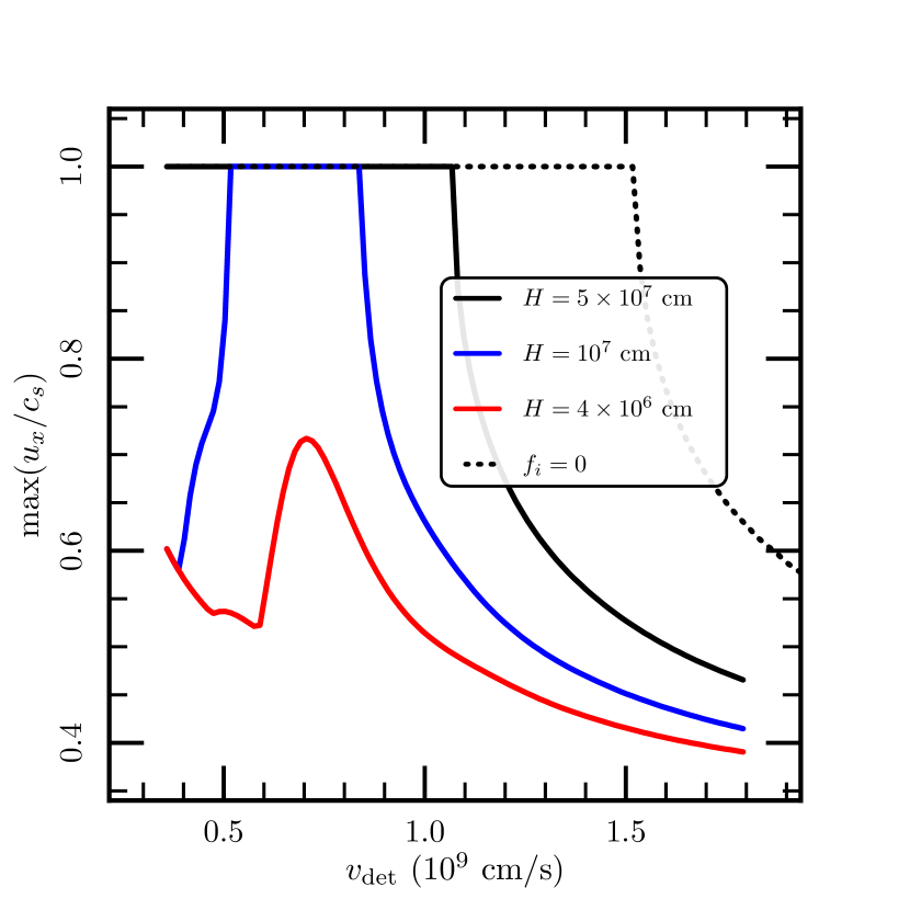
Figure 9.— Maximum mach number ($u_{x}/c_{s}$) achieved in the post-shock flow for pure helium detonations with $\rho_{0}=5\times 10^{5}$ g/cm³ and $T_{0}=10^{8}$ K as a function of detonation velocity, $v_{\rm det}$. Since there is a singularity in the equations at $u_{x}/c_{s}=1$, the integration terminates if there is a sonic point in the post-shock flow at that given $v_{\rm det}$. The dotted line shows the results of a ZND integration with no source terms, while the colored lines show the results when source terms due to blowout and curvature are included for different layer thicknesses parameters, $H$, under the condition $R_{c}=3H$. Detonations that hit a sonic point during burning are possible for all the cases except the $H=4\times 10^{6}$ cm case, since expansion occurs too rapidly for the sonic point to be hit.

The main difference from a normal CJ detonation is that the reactions will freeze out due to expansive effects caused by blowout and/or curvature. Another important difference between a standard CJ detonation and a generalized CJ detonation with source terms is that the burning no longer stops at the singularity for detonations at $v_{\rm gcj}$. Since we are interested in the nucleosynthesis of such detonations we must calculate the additional burning past this singularity, even though the energy released there does not propel the shock front. The ignorance of the final state requires us to guess detonation velocities and use a bisection search to find $v_{\rm gcj}$ for a given set parameters controlling the blowout and curvature source terms, $H$ and $R_{c}$. The situation is that of an eigenvalue problem as described in Sharpe (1999). The sonic point in such a detonation at $v_{\rm gcj}$ is called the pathological point, and is a saddle point in the sense that any integration path with $v_{\rm det}$ either too high or too low is repelled from it. At the pathological point, the post-shock structure bifurcates into either a frozen subsonic solution ($u_{x}<c_{s}$) or a frozen supersonic solution ($u_{x}>c_{s}$) for flow beyond the pathological point.

For a fixed set of initial thermodynamic and compositional conditions, each value of $v_{\rm det}$ will correspond to a different set of post-shock initial conditions for the generalized ZND equations. The source terms require additional information, namely the ambient thickness of the medium, $H$, and the radius of curvature of the detonation front, $R_{c}$. We show the behavior of solutions around the pathological point with $v_{\rm det}$ near $v_{\rm gcj}$ graphically in Figure 10. Each line style corresponds to a pair of $v_{\rm det}$ values that are within a certain tolerance of $v_{\rm gcj}$ $(10^{-2}-10^{-4})$ as determined by a bisection search. Numerical solutions will never reach the pathological point since it is a saddle point, but we can get arbitrarily close by picking a sufficiently stringent tolerance. Solutions with $v_{\rm det}<v_{\rm gcj}$ hit a sonic point and terminate, while solutions with $v_{\rm det}>v_{\rm gcj}$ always remain subsonic. In order to reach the branch where the flow is supersonic with respect to the shock front (the freely propagating solution), we need to traverse the pathological point.

Numerical integration of a system of ODEs containing a coordinate singularity is a challenge. Before we go on, it is useful to examine another way of writing the conditions of a CJ (and generalized CJ) detonation. For a normal CJ detonation, the condition that the flow hits the sonic point when burning is complete means that the numerator and denominator of equation (14) both go to zero at the same time. When we move to the generalized CJ velocity, we are effectively requiring the numerator and denominator of equation (30) to go to zero at the same place - the pathological point. This implies that the thermodynamic derivatives are defined near the pathological point. Although we can never reach the pathological point in a numerical integration, we can get arbitrarily close, and use the fact that the thermodynamic derivatives are well-behaved around the pathological point to linearize our solution past the pathological point. Figure 10 shows how choosing tighter bounds on the integration velocity allows us to linearize the equations closer to the pathological point.

We traverse the pathological point via the following linearization method, similar to that of Sharpe (1999). Given a set of blowout and curvature parameters $(H,R_{c})$ we find the eigenvalue detonation velocity, $v_{\rm gcj}$, to a tolerance of a part in $10^{-5}$. We then use the lower bound velocity (which hits a sonic point slightly before the true pathological point), and integrate the generalized ZND equations until we get close to the sonic point (typically a mach number limit of $\sim 0.99$ is used). We then linearize the generalized ZND equations over a length given by $10-50\%$ of the current $x$ coordinate and resume integration, now on the frozen supersonic branch. The difference between the frozen subsonic and frozen supersonic solutions can be dramatic, requiring us to traverse the pathological point and find the frozen supersonic solution since self-sustaining detonations are frozen supersonic. The resulting solutions for a specific case are shown in Figures 11 & 12. The frozen subsonic solutions shown in dashed lines require supporting pressure behind the pathological point to keep the flow subsonic relative to the shock front. The flow velocity $u_{x}$ goes to zero, indicating that the burned material is traveling at the same speed as the shock front. The thermodynamic derivatives are seen to be discontinuous across the pathological point for the frozen subsonic solution, while they are continuous along the frozen supersonic branch.

Once we have a full frozen supersonic solution, knowing the relative strengths of the source terms due to blowout and curvature along the solution will tell us where each physical effect is important. Recall that our derivation of the curvature source terms assumed that we were in the limit of $x\ll R_{c}$, while the blowout source terms had no such restriction. Figure 13 shows that the blowout source terms become dominant when we are out of the range of validity for the curvature source terms, making the curvature source terms inconsequential. This allows us to integrate the generalized ZND equations beyond the $x\ll R_{c}$ limit and be confident in our results. We leave the curvature terms turned on for calculational simplicity, but they could be turned off around $x\approx R_{c}$ without affecting the integration.

Figure 10.— Thermodynamic variables near the pathological point for a pure helium detonation with initial conditions $\rho_{0}=5\times 10^{5}$ g/cm³, $T_{0}=10^{8}$ K and source term parameters $H=10^{7}$ cm, $R_{c}=3\times 10^{7}$ cm - resulting in a detonation velocity of $v_{\rm gcj}=8.418\times 10^{8}$ cm/s. The broken lines correspond to integrations using detonation velocities given by the bracketing velocities in a bisection search for $v_{\rm gcj}$. Integrations for $v_{\rm det}$ greater/less than $v_{\rm gcj}$ are shown using tolerances of $10^{-2}$ (long dashed lines), $10^{-3}$ (medium dashed lines), and $10^{-4}$ (short dashed lines). The solid line is the eigenvalue solution described in the text using a velocity within $10^{-5}$ of $v_{\rm gcj}$ and linearized when the mach number reached $0.98$, indicated by the solid dot. Detonation velocities less than $v_{\rm gcj}$ hit a sonic point, while those greater than $v_{\rm gcj}$ lie on the frozen subsonic branch.

Figure 11.— Thermodynamic variables for a pure helium detonation with initial conditions $\rho_{0}=5\times 10^{5}$ g/cm³, $T_{0}=10^{8}$ K and source term parameters $H=10^{7}$ cm, $R_{c}=3\times 10^{7}$ cm - resulting in a detonation velocity of $v_{\rm gcj}=8.418\times 10^{8}$ cm/s. Solid lines correspond to the solution that traverses the pathological point and becomes frozen supersonic beyond it, while dashed lines correspond to the frozen subsonic solution. The vertical dotted lines indicate where the solution was linearized to jump over the pathological point.

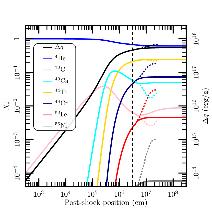
Figure 12.— Nucleosynthesis for a pure helium detonation with initial conditions $\rho_{0}=5\times 10^{5}$ g/cm³, $T_{0}=10^{8}$ K and source term parameters $H=10^{7}$ cm, $R_{c}=3\times 10^{7}$ cm - resulting in a detonation velocity of $v_{\rm gcj}=8.418\times 10^{8}$ cm/s. Colored lines are abundances (left axis) and the black line is the cumulative energy release, $\Delta q$ (right axis). Solid lines correspond to the solution that traverses the pathological point and becomes frozen supersonic beyond it, while dotted lines correspond to the frozen subsonic solution. The vertical dashed line indicates where the equations were linearized to jump over the pathological point.

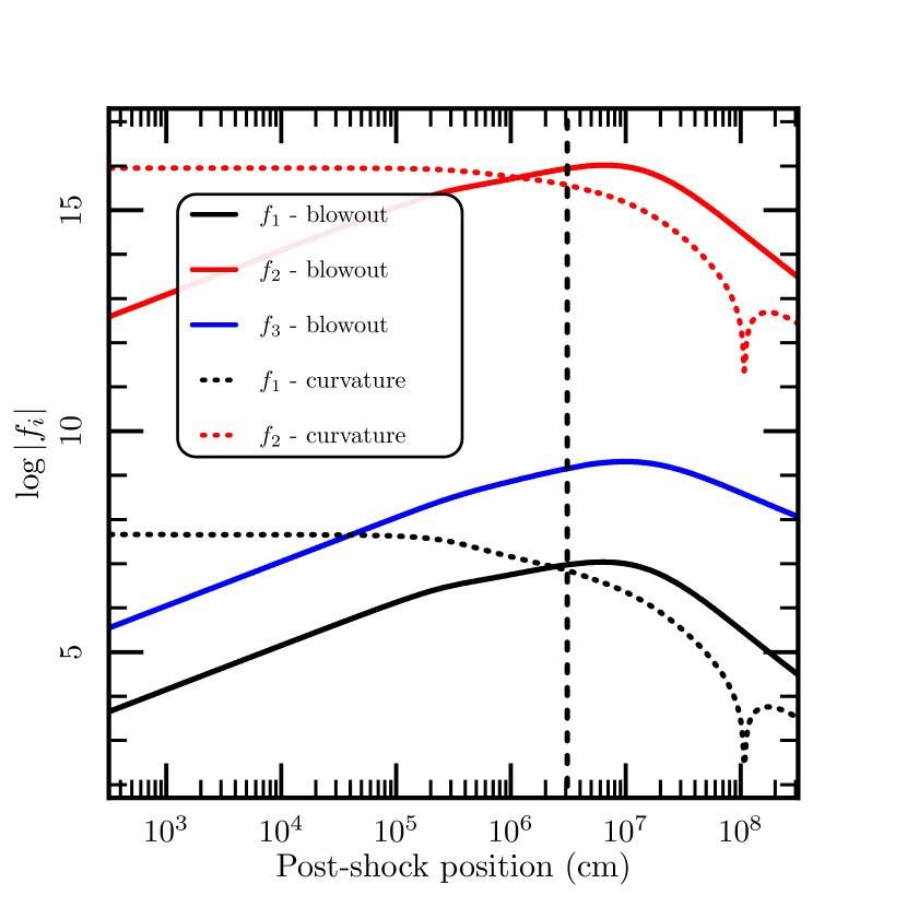
Figure 13.— Absolute values of source terms $f_{1}-f_{3}$ due to blowout (solid lines) and curvature (dotted lines) as a function of distance behind the shock front for a pure helium detonation with initial conditions $\rho_{0}=5\times 10^{5}$ g/cm³, $T_{0}=10^{8}$ K and source term parameters $H=10^{7}$ cm, $R_{c}=3\times 10^{7}$ cm. Note that $f_{3}=0$ for curvature. The vertical dashed line indicates where the equations were linearized to jump over the pathological point. All terms start negative, but the curvature terms switch sign when $u_{x}=v_{\rm det}$ at $x\approx 10^{8}$ cm. At early times, the velocity divergence due to curvature is the important modification to the ZND equations, while at late times blowout dominates.

The generalized CJ velocity corresponds to the steady-state detonation velocity when the expansive effects of blowout and curvature are considered. We need to check and calibrate our 1D prescription using multidimensional hydrodynamic simulations of steady laterally propagating detonations in order to make sure our treatment of blowout is reasonable. The next section details our comparisons between the 1D integrations and FLASH models.

5. Comparisons at constant density

Our goal is to use our 1D ZND model with curvature and blowout to predict detonation speeds and nucleosynthesis. Although the 1D model is physically motivated, it remains a prescription for simulating multidimensional expansive effects. Hence, in this section we compare its predictions to those from reactive compressible hydrodynamic simulations in FLASH. Analysis of FLASH simulations in finite gravity atmospheres led us to investigate a simpler constant density scenario, as described in §3, so our comparisons begin with those models. FLASH simulations use the aprox13 reaction network, while our 1D model uses aprox19 (Timmes, 1999). These networks are effectively identical for the regimes of helium burning we investigate (aprox19 has additional reactions for H burning and photodisintegration, both of which are unimportant in the detonations we consider due to reaction freeze out). We first describe how we relate the curvature of the detonations front, $R_{c}$, to the layer thickness, $H$, reducing the number of free parameters by one. We then compare detonation velocities, nucleosynthesis, and thermodynamic profiles resulting from the 1D generalized ZND equations of section §4 to those from 2D plane-parallel FLASH simulations with helium layers of various densities, thickness, and compositions. We finally summarize the regions of $(\rho_{0},H)$ space where steady detonations can propagate for various compositions.

We developed a treatment of curvature and blowout in the previous sections, with each effect adding an additional length scale - $R_{c}$ for curvature, and $H$ for blowout. Steady detonations in constant density layers have shock fronts with well-defined curvature, as evident in Figure 8. Empirically, we found that the detonation fronts have a radius of curvature that relates to the layer thickness as $R_{c}\approx 3H$. This was found through a large set of constant density FLASH simulations. From here on, we use this relation so that there is only one independent parameter controlling the rate of post-shock expansion, $H$. The parameters left to vary are the initial density, $\rho_{0}$, composition, ${\bf X_{0}}$, and layer thickness, $H$.

5.1. Comparisons between 2D simulations and 1D analytics

The first and simplest point of comparison is the steady-state detonation velocity in a helium layer of varying thickness, $H$, and initial density, $\rho_{0}$. We performed FLASH simulations with helium layers with various initial abundances of ¹²C and ¹⁶O having $\rho_{0}=5\times 10^{5}$ g/cm³ and $H=10^{6}-10^{9}$ cm, finding steady-state detonation velocities of $v_{\rm gcj}=0.59-1.37\times 10^{9}$ cm/s. Each layer thickness yields a unique detonation velocity, $v_{\rm gcj}$, as described in §4.1. This generalized CJ velocity continuously connects to the standard CJ detonation velocity in the $H\rightarrow\infty$ limit. Resolution studies of the FLASH simulations indicate that a spatial resolution of $0.6$ km is sufficient for determining the steady-state detonation speed, with slightly smaller detonation velocities found for coarser resolutions.

The lines in Figure 14 show generalized CJ velocities using $\rho_{0}=5\times 10^{5}$ g/cm³ as a function of $H$ for a few characteristic initial compositions, along with points corresponding to individual 2D FLASH simulations. The minimum in $H$ for each composition shows that steady detonations cannot exist for layers that are too thin - the post-shock expansion occurs so quickly that the pathological point cannot be reached and the flow always remains frozen subsonic. This means that the post-shock rarefaction can communicate back to the shock front and quench the detonation, stopping it from propagating. This effect can also be seen in Figure 9, where decreasing $H$ (also under the assumption $R_{c}=3H$) eventually prevented solutions from hitting a sonic point in the post-shock flow. We observe a similar effect in the FLASH simulations, where reducing the layer thickness beyond a point does not allow us to ignite steadily propagating detonations. We report the detonation limits on $H$ found in FLASH with vertical dashed lines in Figure 14, indicating the thickest layer that failed to yield a propagating detonation for each composition. The slower detonations in ⁴He + ¹⁶O mixtures having speeds around $0.6\times 10^{9}$ cm/s are difficult to realize in hydrodynamic simulations at this density due to stability considerations, but we found them to be realizable at lower densities. Such detonations only burn up to ²⁸Si and can be unstable in the sense that small fluctuations in post-shock temperature can allow burning further up the alpha chain (typically to ⁴⁰Ca), thereby increasing the detonation velocity. A steady-state model will not capture this effect, however, and predicts such detonations to occur. This is consistent with the broader extent at lower densities of the regime in which burning terminates at ²⁸Si before dominance of ⁴⁰Ca (see §5.4).

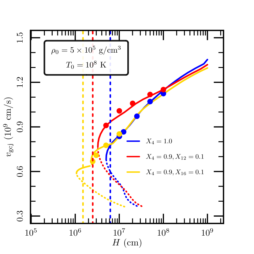
Figure 14.— Generalized CJ velocities as a function of initial layer thickness $H$, using $R_{c}=3H$, for various initial compositions. The initial thermodynamic conditions were $\rho_{0}=5\times 10^{5}$ g/cm³ and $T_{0}=10^{8}$ K for all cases. Solid line segments indicate $v_{\rm gcj}$ values, while the dotted sections correspond to the unphysical solutions at lower detonation velocities (corresponding to the low-velocity side of the cliff in Figure 9). Note the small secondary forbidden region of $v_{\rm gcj}$ for $X_{16}=0.1$ at $H\approx 2.5\times 10^{7}$ cm. Colored dots correspond to individual realizations in FLASH, showing good agreement between our 1D model and direct numerical simulation. The vertical dashed lines indicate the thickest layer in which a detonation would not propagate in FLASH.

Since the detonation velocities are in good agreement with our 1D models, we now move to post-shock structure comparisons. We first note the strong sensitivity of nucleosynthesis on detonation velocity via the initial post-shock conditions - mainly temperature. Small changes in $v_{\rm det}$ ($\sim 1\%$) can produce very large changes in the final product mass fractions ($\sim 100\%$), as Figure 15 shows, so we do not expect to see very close agreement between FLASH models and our 1D models, a priori. To show that our spectrum of solutions is reasonable, we compare the FLASH nucleosynthesis of a pure helium layer with a 1D model using the same thickness in Figure 16. In order to obtain smoother quantities for comparison to 1D, abundances and thermodynamic quantities from FLASH are averaged perpendicular to the direction of propagation over a region within $4\times 10^{6}$ cm of the symmetry plane shown in Figure 7. This is approximately the width of the cellular detonation structures observed in Figure 8. The close agreement shows that our equations describing the post-shock expansive effects are capturing the relevant physics. Thermodynamic comparisons are shown in Figure 17, again showing that the post-shock evolution is well described by our 1D model.

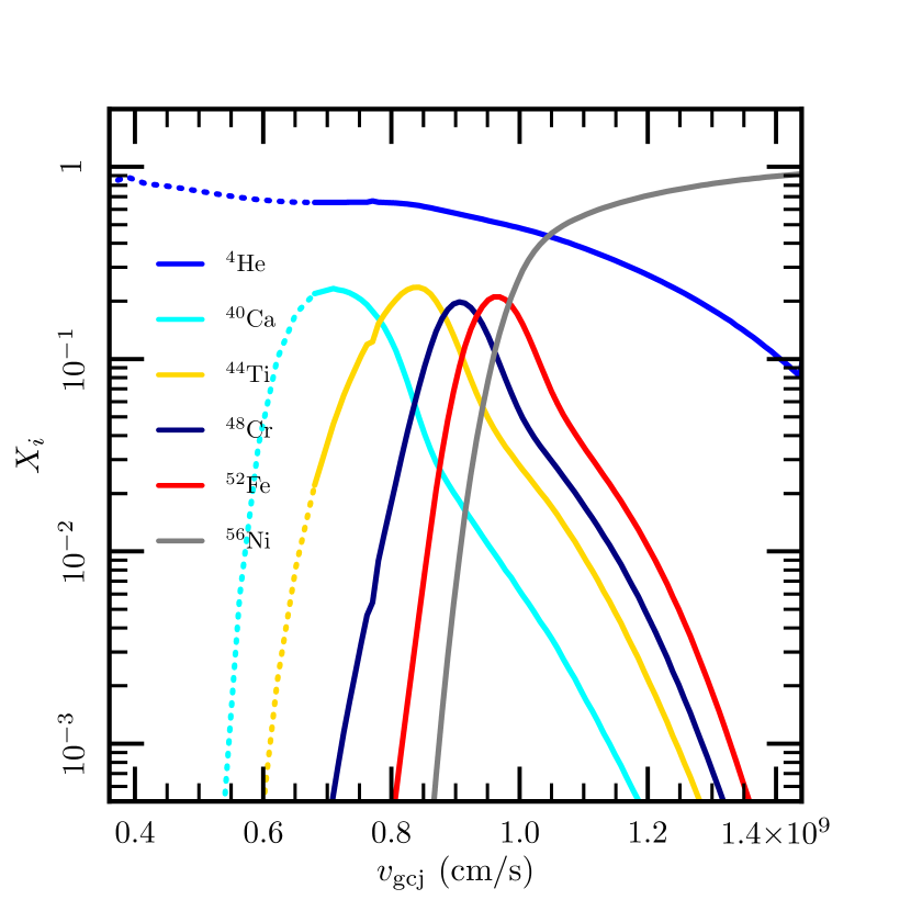
Figure 15.— Final abundances of a pure helium detonation with $\rho_{0}=5\times 10^{5}$ g/cm³ and $T_{0}=10^{8}$ K in the generalized 1D ZND model. As shown in Figure 14, each value of $v_{\rm gcj}$ corresponds to a different $H$, necessary to make that detonation velocity the generalized CJ velocity.

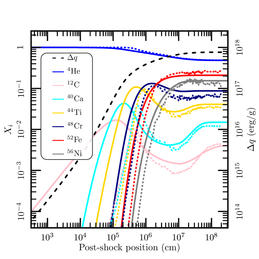
Figure 16.— Nucleosynthesis comparisons between a FLASH model with $\rho_{0}=5\times 10^{5}$ g/cm³, thickness $H=2.5\times 10^{7}$ cm, and steady-state detonation velocity $v_{\rm FLASH}=0.97\times 10^{9}$ cm/s (dotted lines) and a 1D generalized ZND integration using the same initial conditions, also finding $v_{\rm gcj}=0.97\times 10^{9}$ cm/s (solid lines). The dashed black line is the cumulative energy release, to be read off the right axis. Since the FLASH simulation has a resolution of $0.6$ km, the early-time nucleosynthesis is slightly different from the 1D model, although they reach very nearly the same final state.

Figure 17.— Thermodynamic comparisons between a FLASH model with $\rho_{0}=5\times 10^{5}$ g/cm³, thickness $H=2.5\times 10^{7}$ cm, and steady-state detonation velocity $v_{\rm FLASH}=0.97\times 10^{9}$ cm/s (dotted lines) and a 1D generalized ZND integration using the same initial conditions, also with $v_{\rm gcj}=0.97\times 10^{9}$ cm/s (solid lines). The early-time variations are mainly due to the finite resolution ($0.6$ km) of the FLASH simulations.

5.2. Impact of carbon and oxygen in the fuel

We now investigate the effects of adding ¹²C and ¹⁶O to the initial fuel. There are a number of ways in which these isotopes may be produced. First, in the convective burning period prior to the helium shell going dynamical ($t_{\rm burn}<t_{\rm dyn}$), significant amounts of ¹²C + ¹⁶O (5-20% by mass) may be synthesized before a detonation is ignited (Shen & Bildsten, 2009). Additionally, interaction of the base of the convective zone with either the core of the WD or the layer of C/O ashes from previous shell flashes may mix carbon/oxygen into the reaction zone. Similar mixing could occur along the base of the laterally propagating detonation wave as well. Finally, accretion scenarios from helium burning stars allow the composition of accreted material to contain ¹²C and ¹⁶O (Yungelson, 2008).

We have already seen in Figure 14 that the range of allowable detonation velocities and layer thicknesses varies greatly with initial composition. The overall effect of adding ¹²C and ¹⁶O to the fuel can be seen in Figure 18, which shows the lifetimes of several nuclei on the $\alpha$-chain as a function of temperature. While the triple-$\alpha$ rate is relatively flat over this temperature range, $\alpha$-captures on nuclei going up the $\alpha$-chain are quite sensitive to temperature. Typical post-shock temperatures for generalized CJ detonations with characteristic layer thicknesses are $1-3\times 10^{9}$ K as shown in Figure 19. For these temperatures, $\alpha$-captures on ¹⁶O up to ²⁸Si are much faster than both the triple-$\alpha$ process and $\alpha$-capture onto ¹²C. We therefore expect any ¹⁶O in the initial fuel to burn to ²⁸Si very quickly. Rapid $\alpha$ captures onto ¹⁶O can dramatically decrease the burning length scale, $l_{95}$, and therefore reduce the minimum layer thicknesses that allows for steady detonations as well as the speeds of such detonations. Figures 20 and 21 show the reaction length scale, $l_{95}$, and distance to the pathological point. Our intuition from Equation (26) suggests that the small energy release allows for extremely low detonation velocities. We check this scaling in Figures 22 and 23, where we plot the net energy release, $\Delta q$, against the generalized CJ velocity for various compositions. We find that $\Delta q$ scales as expected, albeit with some deviation at low velocities for cases with $10\%$ ¹⁶O in the fuel.

From Figures 22 and 23, we see that while a ¹⁶O mass fraction of $X_{16}=0.05$ does not produce a large reduction in the minimum $v_{\rm gcj}$, a mass fraction of $X_{16}=0.1$ does. We can estimate the minimum mass fraction of ¹⁶O required to dramatically change the detonation structure as follows. The post-shock temperature range where ¹⁶O can burn to ²⁸Si before any other reactions take place is (from Figure 18) $T_{N}\gtrsim 0.9\times 10^{9}$ K. This temperature corresponds to a shock strength given by a detonation with $v_{\rm det}\approx 0.6\times 10^{9}$ cm/s, from Figure 19. We can estimate the energy release from a detonation at that velocity using Equation (26). We use $\gamma=5/3$ since this is a relatively weak shock, and the post-shock conditions will not be radiation-dominated ($P_{\rm rad}/P_{\rm gas}\approx 10^{-2}$). This yields a minimum $\Delta q\approx 10^{17}$ erg/g for ¹⁶O to ²⁸Si burning to dominate the early-time energy release. The energy released from only burning ¹⁶O to ²⁸Si in terms of the initial mass fraction of ¹⁶O is

$$\Delta q\left({}^{16}{\rm O}\rightarrow^{28}{\rm Si}\right)= \left[\left(1-\frac{7}{4}X_{16}\right)\frac{Q_{4}}{A_{4}}+\frac{7}{4}X_{16}\frac{Q_{28}}{A_{28}}\right]-$$

$$\left[\left(1-X_{16}\right)\frac{Q_{4}}{A_{4}}+X_{16}\frac{Q_{16}}{A_{16}}\right].$$ (33)

We can find the mass fraction $X_{16}$ that allows for a detonation strong enough that the post-shock temperature allows for burning of ¹⁶O to ²⁸Si before anything else, giving

$$X_{16}=\frac{\Delta q}{\frac{7}{4}Q_{28}-Q_{16}-\frac{3}{4}Q_{28}}\approx 0.07,$$ (34)

in good agreement with the behavior observed at lowest values of $v_{\rm gcj}$. Based on the $\alpha$-capture timescales in Figure 18, we expect to see similar effects if ²⁰Ne or ²⁴Mg are present in the fuel, as they are nearly interchangeable with ¹⁶O in terms of burning speed for the low temperatures relevant here, but release less energy when burning to ²⁸Si.

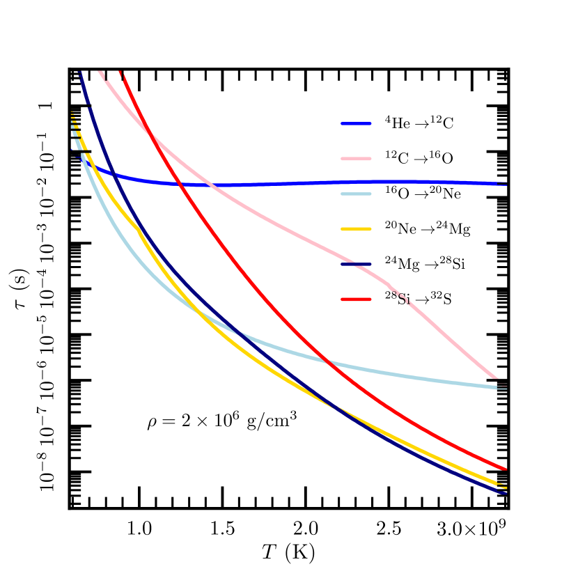
Figure 18.— Lifetimes of various $\alpha$-chain nuclei against $\alpha$-capture, including both $(\alpha,\gamma)$ and $(\alpha,p)(p,\gamma)$ channels, computed using pure ⁴He at a density of $\rho=2\times 10^{6}$ g/cm³. The lifetimes are defined as $\tau_{i}=(n_{\alpha}\left<\sigma v\right>_{i})^{-1}$, where $n_{\alpha}$ is the number density of $\alpha$ particles, and $\left<\sigma v\right>_{i}$ is the net velocity-averaged $\alpha$-capture cross section onto the $i^{\rm th}$ species.

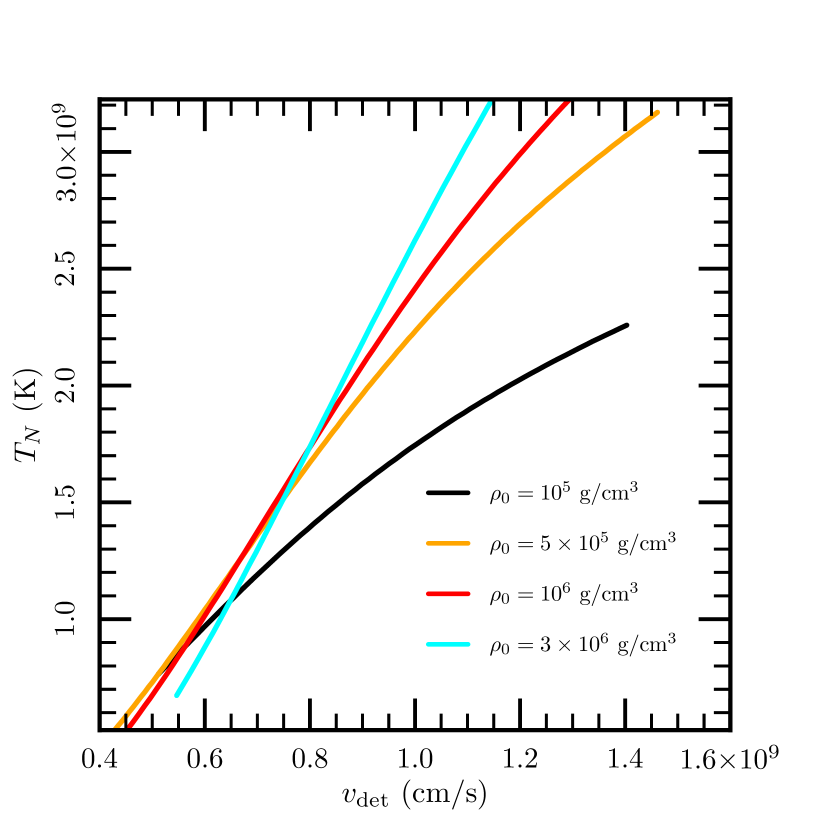
Figure 19.— Post shock temperature ($T_{N}$) as a function of detonation velocity for a variety of initial densities. $T_{N}$ only depends on the shock jump conditions, so we label the $x$-axis as $v_{\rm det}$ since these jump conditions do not always correspond to generalized CJ detonations.

Figure 20.— Various length scales for generalized CJ detonations in layers having $\rho_{0}=5\times 10^{5}$ g/cm³ and various initial compositions down to $90\%$ helium. Solid lines are $l_{95}$, the length scale over which $95\%$ of the nuclear burning energy is released. Dashed lines correspond to the distance behind the shock front to the pathological point.

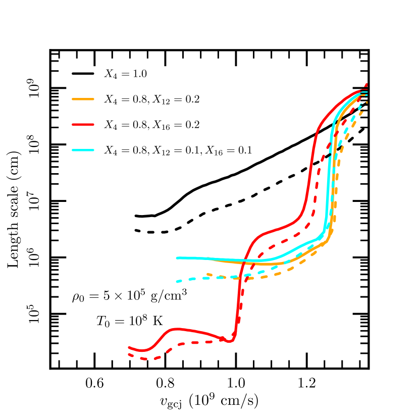
Figure 21.— Same as Figure 20, but with compositions down to $80\%$ helium by mass.

Figure 22.— Detonation energy release $\Delta q$ as a function of generalized CJ velocity, $v_{\rm gcj}$, for detonations in layers having $\rho_{0}=5\times 10^{5}$ g/cm³, $T_{0}=10^{8}$ K, and various initial compositions down to $90\%$ helium by mass.

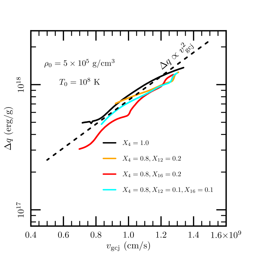
Figure 23.— Same as Figure 22, but with compositions down to $80\%$ helium by mass.

5.3. Larger reaction networks

An advantage of our 1D model is that it allows us to use much larger reaction networks than those feasible in FLASH. Recall FLASH is using a 13-isotope alpha chain (aprox13), and for our comparisons to FLASH we use a 19-isotope alpha chain with the addition of ¹H, ³He, ¹⁴N, ⁵⁴Fe, along with special neutrons and protons for photo-disintegration. Both helium white dwarf donors and non-degenerate helium burning star donors are expected to have significant enrichments (up to few percent) of ¹⁴N due to CNO burning earlier in the star’s life, which can be important in explosive helium burning through production of ¹⁴C (Hashimoto et al., 1986). In this section we examine the predictions made with a larger $136$-isotope reaction network, as well as the effects of adding initial ¹⁴C to the helium. As discussed in Shen & Bildsten (2009), the neutron/proton ratio at the onset of dynamical burning in a helium envelope is fixed at the beginning of the convective burning phases since there is not enough time for electron captures to happen before the burning becomes dynamical. We therefore expect any ¹⁴N or ¹⁴C excess from CNO burning to be relevant to a detonation if one develops.

We first compare the nucleosynthesis of the $136$-isotope network with that of the $19$-isotope network for pure helium detonations with identical initial conditions ($\rho_{0}=5\times 10^{5}$ g/cm³, $H=2.5\times 10^{7}$ cm) in Figure 24. In general, different reaction networks will give different generalized CJ velocities because the energy release rate plays a critical role in determining the detonation structure. However, both of these networks give the same detonation velocity, $v_{\rm gcj}=0.97\times 10^{9}$ cm/s. The nucleosynthetic profile is slightly different between the two reaction networks, with the main difference being less ⁵⁶Ni production in the $136$-isotope network (offset by production of isotopes such as ⁵⁵Co and ⁵⁷Ni). Both reaction networks finding the same $v_{\rm gcj}$ value means they agree very closely in total energy release, so we can be confident in the detonation velocity predictions using the $19$-isotope network.

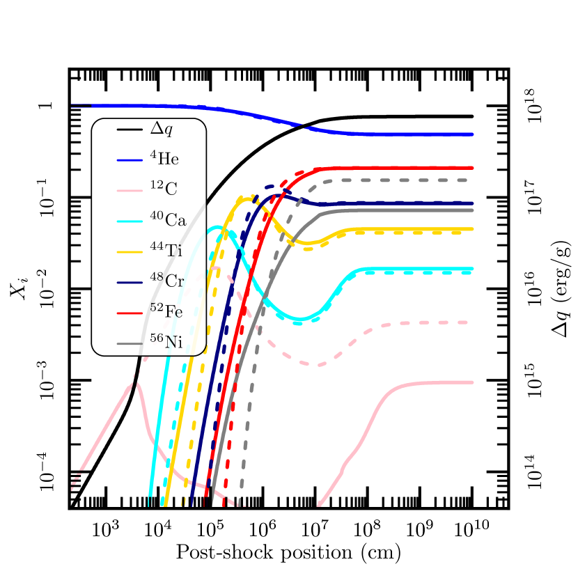
Figure 24.— Solid lines correspond to the post-shock nucleosynthesis and energy release computed with a 136-isotope network for a generalized CJ detonation in pure He and ambient conditions $\rho_{0}=5\times 10^{5}$ g/cm³, thickness $H=2.5\times 10^{7}$ cm, yielding a detonation velocity $v_{\rm gcj}=0.97\times 10^{9}$ cm/s. Dashed lines represent a detonation with the same initial conditions, but in pure Helium using the 19-isotope network as in Figure 16. The decrease in ⁵⁶Ni production in the 136-isotope case is balanced by the production of isotopes such as ⁵⁵Co (unstable, $t_{1/2}=18$h) and ⁵⁷Ni (unstable, $t_{1/2}=36$h).

We now briefly examine the effects of adding neutron-rich isotopes to the fuel. As discussed in Timmes et al. (2003), a small amount of neutron-rich material in the fuel can have a noticeable impact on the final yields of radioactive isotopes such as ⁵⁶Ni. Figure 25 shows the nucleosynthesis of a detonation with the same starting conditions as Figures 16 and 24, but with $2\%$ ¹⁴C by mass added to the fuel. The net effect is production of neutron-rich isotopes such as ⁵³Fe, ⁵⁷Ni, and ⁵⁸Ni. We observe qualitatively similar effects when adding other neutron-rich isotopes such as ¹⁸O or ²²Ne to the fuel.

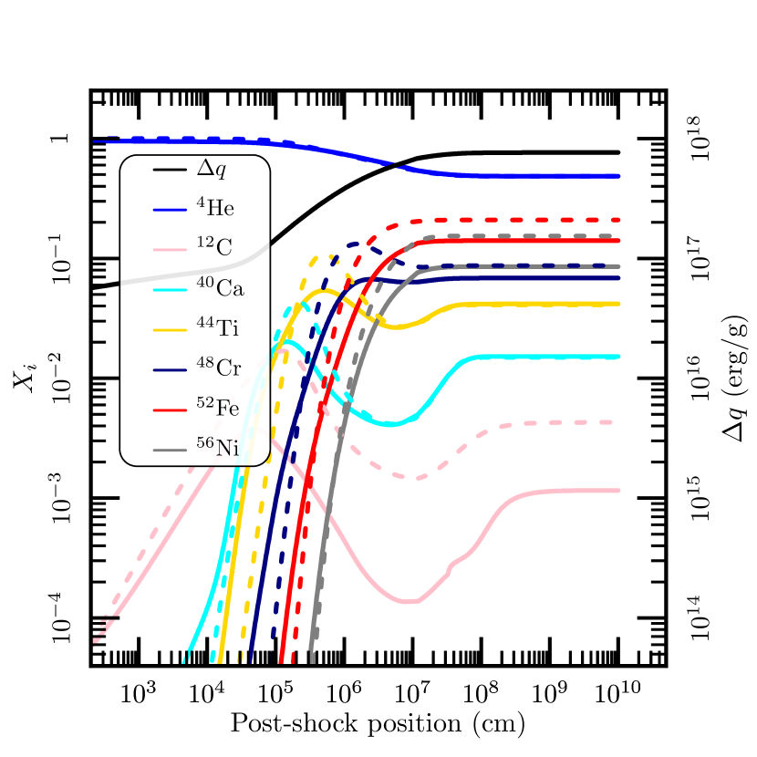
Figure 25.— Solid lines correspond to the post-shock nucleosynthesis and energy release computed with a 136-isotope network for a generalized CJ detonation with a fuel composition of $2\%$ ¹⁴C by mass and $98\%$ ⁴He, and ambient conditions $\rho_{0}=5\times 10^{5}$ g/cm³, thickness $H=2.5\times 10^{7}$ cm, yielding a detonation velocity $v_{\rm gcj}=0.97\times 10^{9}$ cm/s. Dashed lines represent a detonation with the same initial conditions, but in pure Helium using the 19-isotope network as in Figure 16. The case with the slight neutron excess leads to less production of $\alpha$-chain isotopes, but more neutron-rich isotopes such as ⁵³Fe (unstable, $t_{1/2}=8$m), ⁵⁷Ni (unstable, $t_{1/2}=36$h), and ⁵⁸Ni (stable).

5.4. Detonation propagation limits

We showed in Figure 9 that there is a lower limit on the layer thickness that can support a steady detonation for a given $\rho_{0}$ and ${\bf X}_{0}$. We therefore summarize the regions of the $(\rho_{0},H)$ plane where laterally propagating detonations are allowed for a given composition. Figures 26, 27, and 28 show the regions of parameter space where detonations are allowed for initial compositions of $(X_{4}=1.0)$, $(X_{4}=0.9,\ X_{12}=0.1)$, and $(X_{4}=0.9,\ X_{16}=0.1)$, respectively. Colored lines denote where each isotope becomes the dominant burning product. Recall from Figure 15 that the burning products are typically $10-20\%$ by mass until the detonation is strong enough to produce significant amounts of ⁵⁶Ni, so the majority of the material remains unburned helium. Dashed and dotted lines indicate the mass fraction of helium remaining in the ashes. The region below the lowest isotope line does not allow detonation propagation because expansion happens too quickly for a post-shock sonic locus to form. The effects of adding small amounts of ¹²C or ¹⁶O to the fuel are to decrease the minimum thickness $H$ that allows for detonation propagation at any given $\rho_{0}$. In the next section we will show how to translate detonations in $(\rho_{0},H)$ space into finite-gravity helium layers on WDs.

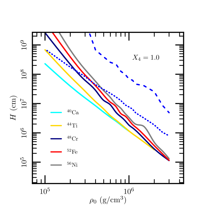
Figure 26.— Regions where laterally propagating detonations in pure helium are possible as a function of initial layer thickness $H$ and density $\rho_{0}$. Regions above the lowest colored line can support generalized CJ detonations, with each point corresponding to a detonation in a layer with different initial conditions. Colors indicate where, as $H$ increases at fixed $\rho_{0}$, each nuclide first becomes the dominant burning product (see Figure 15). Significant amounts of initial helium remain so the dotted blue line shows where the mass fraction of unburned helium is $50\%$ and the dashed blue line shows where the mass fraction of unburned helium is $25\%$. Steady detonations cannot propagate in the region below the lowest isotope lines.

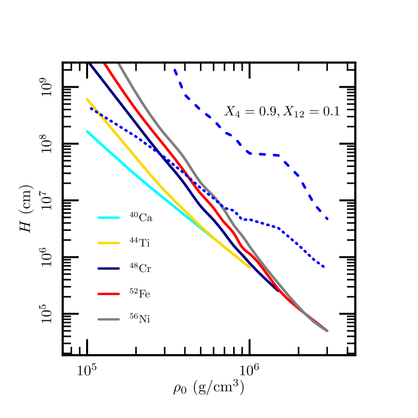
Figure 27.— Same as Figure 26, but for detonations in material composed of $90\%$ ⁴He and $10\%$ ¹²C by mass.

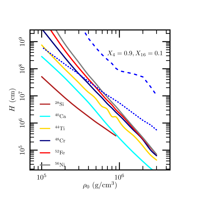
Figure 28.— Same as Figure 26, but for detonations in material composed of $90\%$ ⁴He and $10\%$ ¹⁶O by mass. For this initial composition, the slowest detonations produce more ²⁸Si than other products for initial densities below $10^{6}$ g/cm³.

6. Detonations in finite gravity environments

The results and comparisons in the previous section were presented in terms of the 1D model parameters - $H$ and $\rho_{0}$. We now map these variables to a set of WD core and envelope masses, connecting to the astrophysical scenarios. In this section, we describe a way to map our constant density analytics onto cases with finite gravity, and hence vertical density gradients. We again compare to 2D FLASH models in finite gravity and then present detonation limits in the form of a minimum envelope mass as a function of WD core mass and envelope composition.

6.1. FLASH simulations

The assumptions we make when mapping 1D constant density detonations to detonations in finite gravity arise from analyzing FLASH simulations of detonations in plane-parallel geometry with gravity. Such FLASH simulations show that the leading part of the detonation front lies above the base of the layer (see also Figure 6). Our strategy is to interpret the leading point of the detonation as the leading point of the constant-density detonation - the centerline in Figure 7. We therefore use the layer density and shock curvature at this height as the initial conditions for our 1D model. Empirically, the forwardmost point on the shock front in FLASH occurs at a height roughly $H_{s}/2$ above the base of the layer, where $H_{s}=P_{b}/(\rho_{b}g_{b})$ is the scale height evaluated at the base conditions. We assume a polytrope model for the atmosphere,

$$\frac{P}{P_{b}}=\left(\frac{\rho}{\rho_{b}}\right)^{\gamma},$$ (35)

where $P_{b}$ and $\rho_{b}$ are the pressure and density at the base of the layer, respectively. Combining this with hydrostatic balance, $dP/dz=-\rho g$ ($z$ being the coordinate in the vertical direction), yields

$$\frac{\rho}{\rho_{b}}=\left[1-\left(\frac{\gamma-1}{\gamma}\right)\frac{z}{H_{s}}\right]^{1/(\gamma-1)}.$$ (36)

For a convective or degenerate (non-relativistic) atmosphere, $\gamma=5/3$, and we find $\rho(H_{s}/2)\approx 0.7\rho_{b}$. The curvature of the shock front in the FLASH simulations relates to the layer thickness via $R_{c}\approx 3H\approx 3H_{s}/2$.

We map our calculation parameters $(\rho_{0},H)$ to WD core and envelope masses ($M_{c}$ and $M_{\rm env}$, respectively) as follows. We construct a WD core by integrating the stellar structure equations using the MESA EOS and assuming a fixed temperature ($T_{c}=10^{7}$ K) and composition for the core. The core composition is taken to be equal parts ¹²C and ¹⁶O by mass. Since we assume a constant temperature and composition, we only need the equations of hydrostatic balance and mass conservation along with an equation of state. We use $P$ as our independent variable since the integration bounds are more easily expressed in terms of pressure than radius. The initial conditions are $r(P_{c})=0$ and $M(P_{c})=0$, where $P_{c}$ is the central pressure, a parameter that fixes the structure of the WD core. If we just want to characterize a WD core, we can take an outer boundary at a very low pressure (eg. $P/P_{c}=10^{-6}$) to define the surface of the star. In order to add an envelope, we integrate to a higher pressure ratio $P_{b}/P_{c}>10^{-6}$ corresponding to the base of the envelope, and then switch to an isentropic atmosphere model where the temperature varies as

$$T=T_{b}\left(\frac{\rho}{\rho_{b}}\right)^{\gamma-1},$$ (37)

where $T_{b}$ is the temperature at the base of the convective envelope. Although the pressure is continuous, there is a small jump in density across the core-envelope boundary due to the composition and temperature change. We then integrate the envelope structure out to the outer pressure boundary (eg. $P/P_{c}=10^{-6}$) to calculate the envelope mass. Each WD model is therefore determined by two parameters - the central pressure $P_{c}$, and the pressure ratio at the core-envelope boundary $P_{b}/P_{c}$. We can then extract the density $\rho_{0}$ and thickness $H=P_{b}/(2\rho_{b}g_{b})$ to use in the generalized ZND integrations. Along with our assumption that $R_{c}=3H$, This allows us to map our previous points in $(H,\rho_{0})$ space into $(M_{c},M_{\rm env})$ space and vice-versa.

We end this section by noting that the $T_{b}$ varies depending on the progenitor scenario, with both larger envelope and core masses producing higher $T_{b}$ values before dynamical runaway (Shen & Bildsten, 2009). We take $T_{b}=10^{8}$ K as our fiducial for constructing hydrostatic WD envelopes, with higher temperatures corresponding to lower values of $\rho_{b}$ given the same $M_{c}$ and $M_{\rm env}$. Such envelopes that are hot and massive relative to those in the AM CVn accretion scenario may be relevant in the low accretion rates of a WD + He burning star donor (Yungelson, 2008) or unstable mass transfer during a WD + He WD merger (Guillochon et al., 2010; Schwab et al., 2012; Shen et al., 2012; Pakmor et al., 2013). These hot envelopes are different enough from our hydrostatic WD models that they are better placed in $(H,\rho_{0})$ space, as in Figures 26 - 28.

6.2. Detonation propagation limits on WDs

Figures 29 and 30 show the regions of allowed detonation propagation to WDs. These figures correspond to Figures 26 - 28, but in terms of WD parameters. We again compare to FLASH simulations, this time in finite gravity, with the colored dots corresponding to the most abundant nuclide produced by the forwardmost portion of the detonation in FLASH.

While detonations in constant density strips have some variation in nucleosynthesis in the direction perpendicular to the centerline (see Figure 7), detonations in finite gravity strips also have an initial density gradient in the vertical direction. This produces an even stronger variation in burning products as a function of height. When we refer to final abundances of such detonations, we mean abundances along the centerline of the detonation, a distance $H_{s}/2$ above the base of the layer. Detonation products as a function of height are shown in Figure 31. As in the constant density strips, burning progresses furthest along the centerline, while material higher above burns even less completely. A series of peaks of lighter products as one moves up higher in the layer is characteristic of such detonations with finite gravity. Therefore, Figures 29 and 30 show limits on how far the burning can progress up the $\alpha$ chain. For example, a point that lies in the region where ⁴⁸Cr is the dominant product corresponds to a detonation that produces isotopes up to ⁴⁸Cr, with regions above $H_{s}/2$ burning less completely. We would thus expect to see a stratification of lighter elements outside of heavier elements in the ejecta corresponding to a laterally propagating helium detonation. We plan a more detailed characterization of ejected abundances with full-star detonation simulations in an upcoming paper.

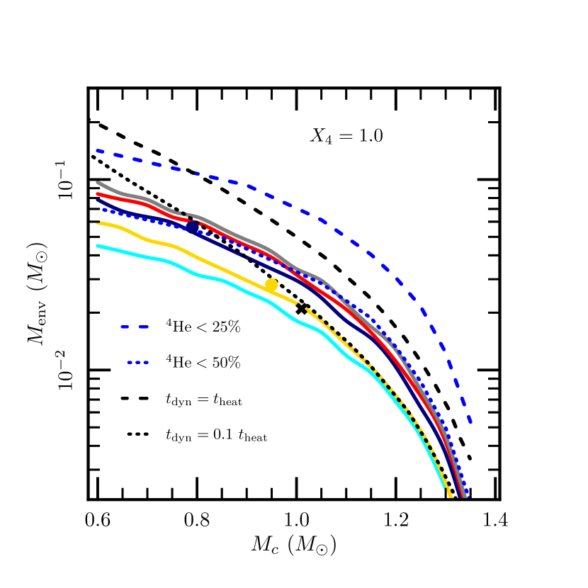
Figure 29.— Regions where laterally propagating detonations in pure helium are allowed as a function of core and envelope mass. Solid lines indicate transitions in dominant burning products as in Figures 26 - 28 in the order (bottom to top): ⁴⁰Ca, ⁴⁴Ti, ⁴⁸Cr, ⁵²Fe, and ⁵⁶Ni. The dotted blue line shows where the mass fraction of unburned helium is $50\%$ and the dashed blue line shows where the mass fraction of unburned helium is $25\%$. Regions below the ⁴⁰Ca line do not allow detonation propagation because expansion happens too quickly for a post-shock sonic locus to form. Black dashed and dotted lines show calculations guiding where dynamical shells are expected by comparing the local heating timescale $t_{\rm heat}$ to the dynamical timescale $t_{\rm dyn}$ from Shen & Bildsten (2009). Dots indicate where we performed 2D FLASH runs with finite gravity and found propagating detonations, with their colors corresponding to the most dominant isotope produced along the centerline of the detonation, while X’s indicates runs where no propagating detonations were found.

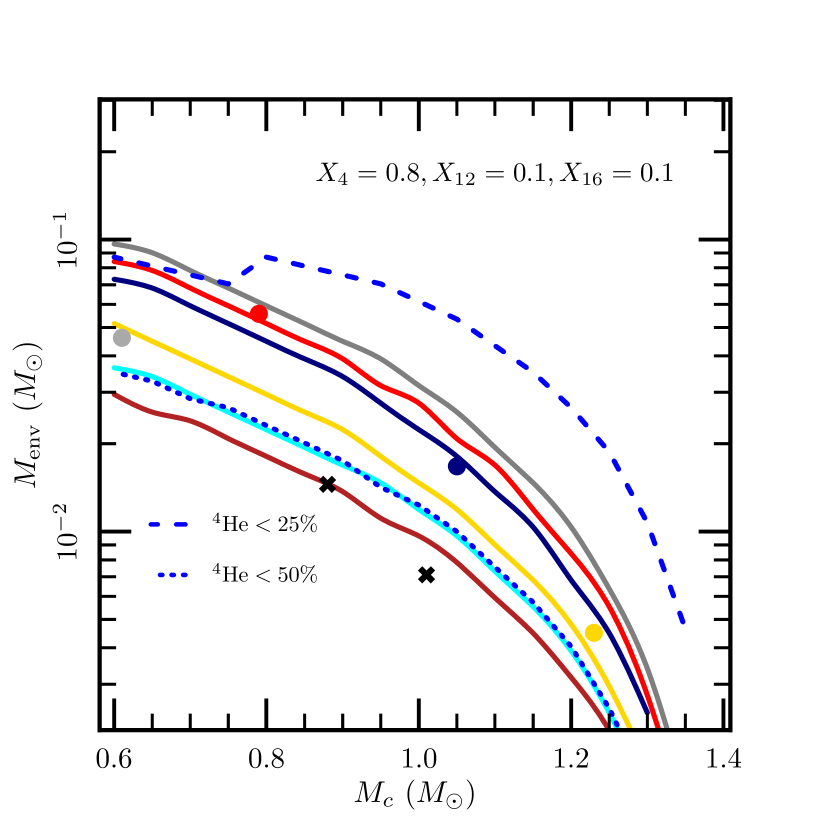
Figure 30.— Same as Figure 29, but with an envelope composed of $80\%$ ⁴He, $10\%$ ¹²C, and $10\%$ ¹⁶O by mass. The lowest solid line here corresponds to ²⁸Si, from the rapid ${}^{16}{\rm O}\rightarrow^{28}$Si reactions. The dot representing the FLASH simulation at $(M_{c}=0.61\ M_{\odot},M_{\rm env}=4.6\times 10^{-2}\ M_{\odot})$ is colored for ³²S production.

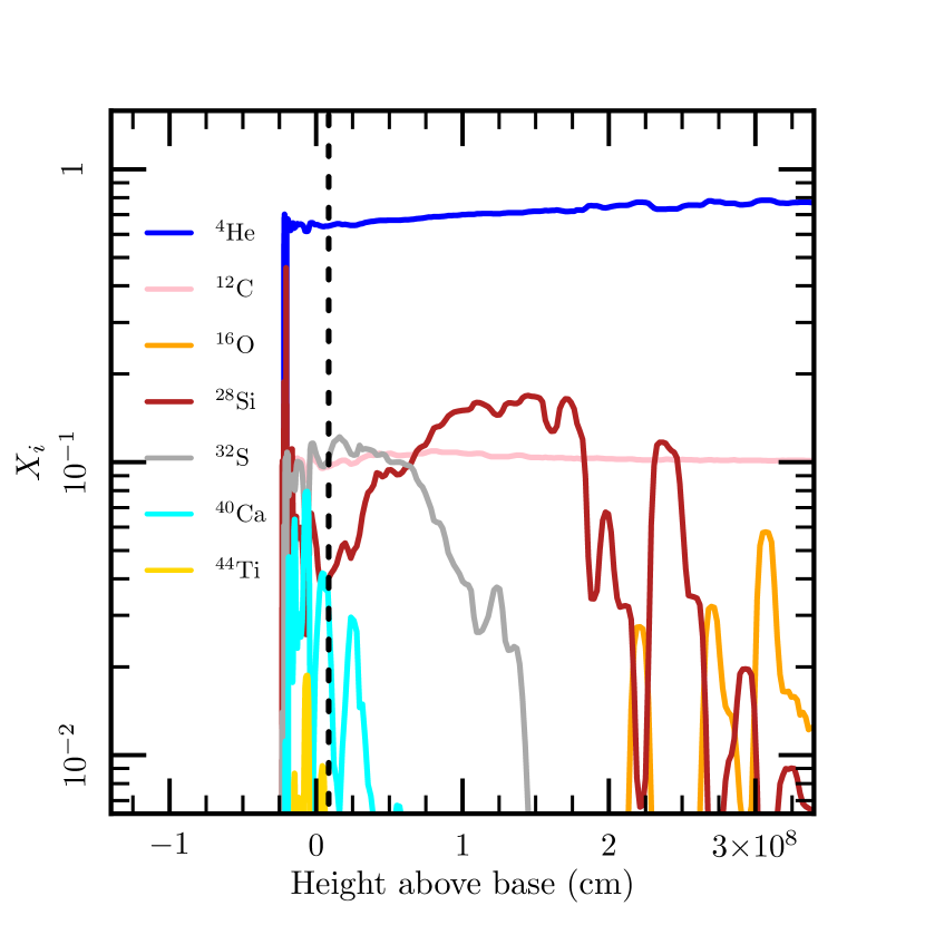
Figure 31.— Vertical abundance profile from a FLASH simulation of a detonation with initial composition $X_{4}=0.8,X_{12}=0.1,X_{16}=0.1$, $\rho_{b}=2\times 10^{5}$ g/cm³, $T_{b}=10^{8}$ K, $g_{b}=2\times 10^{8}$ cm/s², and $H_{s}=6.4\times 10^{7}$ cm. This led to a detonation with velocity $v_{\rm gcj}=0.68\times 10^{9}$ cm/s, corresponding to the grey dot in Figure 30. This abundance profile is taken $10^{8}$ cm behind the detonation front, where burning has ceased. The zero point of the $x$-axis is taken at the initial position of the base of the helium layer, $1.5\times 10^{8}$ cm. Consistent with our assumptions, the most abundant isotopes lie near the centerline of the detonation - indicated by a dashed line a height $H=H_{s}/2$ above the current base of the layer. Elements above ⁴⁴Ti do not appear on this plot because they are not produced in abundances greater than $10^{-2}$.

6.3. Implications for explosion scenarios

We note that nearly all of the parameter space shown is predicted to contain significant amounts ($>25\%$) of unburned helium, and a range of radioactive elements. Detonations near the propagation cutoff line are predicted to produce very little mass in ⁵⁶Ni, with most of the products being intermediate-mass elements (IMEs) such as ⁴⁰Ca, ⁴⁴Ti, etc. This motivates the possibility of extremely faint events that have very low yields of radioactive elements. More detailed investigations of helium detonation ignition in such low densities are necessary to determine whether detonations are likely to form in such environments.

We also examine whether these surface detonations are fast enough to cause inwardly-propagating shock waves to focus in the interior of the C/O core - possibly detonating the core and making a Type Ia SN in a double-detonation scenario. For each successful detonation in $M_{c}-M_{\rm env}$ space, we compute the time it takes the detonation to travel around the WD to the antipode of its initiation point,

$$t_{\rm det}=\frac{\pi R_{c}}{v_{\rm gcj}},$$ (38)

where $R_{c}$ is the radius of the WD core. A lower limit on the time it takes the inwardly-propagating shock waves to traverse the interior of the core is given by the sound travel time through the core,

$$t_{\rm sound}=2\int_{0}^{R_{c}}\frac{dr}{c_{s}}.$$ (39)

We show lines of constant $t_{\rm det}$ and $t_{\rm sound}$ in Figures 32 and 33. Virtually all detonations in these cases are fast enough to allow the inwardly propagating shock waves to focus in the interior of the WD. It remains uncertain whether such focusing allows for a secondary detonation in a C/O or O/Ne/Mg core. Multidimensional simulations typically favor igniting the core (Moll & Woosley, 2013; Sim et al., 2012; Fink et al., 2010) - see also Guillochon et al. (2010), but have a resolution much coarser than the extremely short carbon burning length scale $(\sim 1\ {\rm cm})$. High-resolution 1D calculations indicate that ignition in C/O cores may be possible if the shocks focus within a small enough critical region $(\sim 10^{3}\ {\rm cm})$, but ignition in carbon-deficient environments such as O/Ne/Mg is more difficult and perhaps not realizable with converging shocks in the double-detonation scenario (Shen & Bildsten, 2013; Seitenzahl et al., 2009).

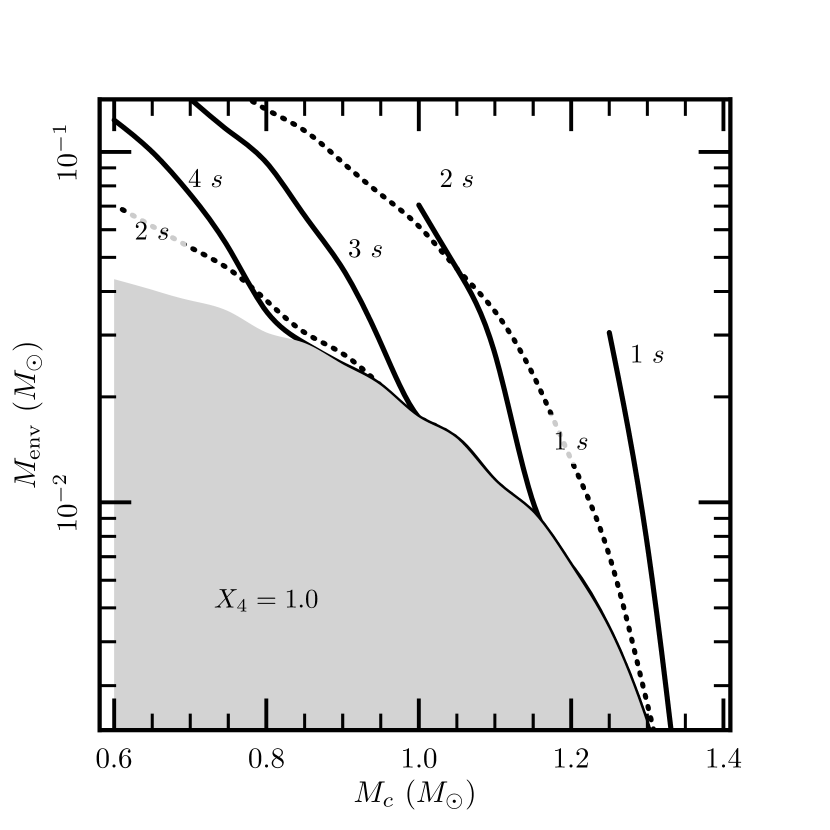
Figure 32.— Lines of constant $t_{\rm sound}$ (solid lines) and $t_{\rm det}$ (dotted lines) for detonations in pure helium envelopes with $T_{b}=10^{8}$ K on WDs in $M_{c}-M_{\rm env}$ space, corresponding to Figure 29. The shaded region indicates where the envelopes are too thin to support steady detonations.

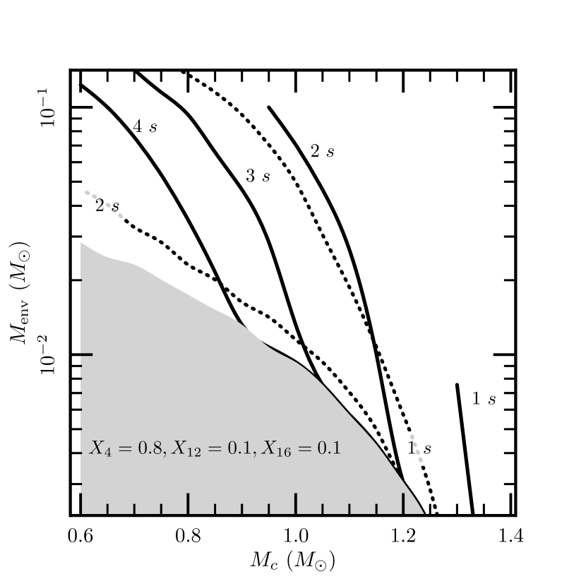
Figure 33.— Same as Figure 32, but with an envelope composition of $80\%$ ⁴He, $10\%$ ¹²C, and $10\%$ ¹⁶O by mass, corresponding to Figure 30.

7. Conclusions

Standard CJ detonations are not realizable in the low-density environments of thin helium shells on accreting WDs. Instead, a class of solutions, the generalized CJ solution (He & Clavin, 1994) with $v_{\rm gcj}<v_{\rm CJ}$, determined by the expansive effects of curvature and blowout in the post-shock burning regions, is allowed in helium envelopes with large enough thicknesses. We constructed a 1D model of such detonations by adding these expansive effects into the ZND equations describing the evolution of shocked material as it burns behind the detonation front. Comparisons to 2D detonation simulations with FLASH indicate that we are capturing the relevant physics in the post-shock material with our 1D model. We find both minimum thicknesses allowing for detonation propagation and important reductions in burning length scales when isotopes such as ¹⁶O, ²⁰Ne, and ²⁴Mg are added to the fuel. Dredge-up from O/Ne/Mg WDs is thus expected to have more of an impact on nucleosynthesis than in C/O WDs.

We can map our 1D models to FLASH models in finite gravity, and predict which WD core + envelope configurations will support steady detonations. We can calculate the composition of the most burned section of the envelope with our 1D model, but specific vertical profiles of composition require multidimensional simulations. While detonations in pure helium generate enough energy to become unbound from the WD, the ashes from the very slowest ¹⁶O-enabled detonations are only barely gravitationally unbound, something we intend to more fully consider in future work. Our 1D model also neglects how the global curvature of the WD affects the detonation velocity - weakening as it approaches the equator and then strengthening towards the other pole due to divergence/convergence of the detonation front. We plan on addressing this and related issues in a future paper with full-star axisymmetric simulations in FLASH.

We have examined criteria allowing for the propagation of surface detonations, but have not touched on the important problem of detonation initiation in helium. Detailed investigation is necessary to determine if detonations can be ignited in some of the low-density environments considered here. The reduction in burning length scales in detonations with sufficient ¹⁶O abundances may allow detonations in helium shells to occur in a wider range of envelopes than originally considered in pure helium (Holcomb et al., 2013).

We thank Ryan Foley, Dan Kasen, Bill Paxton, and Ken Shen for useful discussions and the anonymous referee for helpful comments. This work was supported by the National Science Foundation under grants PHY 11-25915 and AST 11-09174. Some of the software used in this work was in part developed by the DOE-supported ASC/Alliances Center for Astrophysical Thermonuclear Flashes at the University of Chicago. Some of the simulations for this work were made possible by the Triton Resource, a high performance research computing system operated by San Diego Supercomputer Center at UC San Diego.

Appendix A Modeling curvature in 1D

The curvature of the detonation front affects the generalized CJ velocity due to the divergence in velocity immediately behind the shock front. The theory of detonation shock dynamics (DSD) (Bdzil & Stewart, 2012), allows us to relate the curvature of the shock front to the detonation velocity through source terms in the hydrodynamic equations, similar to how curvature was modeled in 1D by Dursi & Timmes (2006). He & Clavin (1994) also investigated the effects of curvature on detonation ignition and propagation speed, assuming a complete burn and a single-step reaction. We can adapt their treatment to the case of partial burning with blowout using our reaction networks. We work in the weak curvature limit here, $l_{95}\ll R_{c}$, where $R_{c}$ is the radius of curvature of the detonation front, but will justify a unified approach that allows for integration past this limit when we discuss radial expansion in the next section. To derive the source terms we start with a simple 1D geometry with planar, cylindrical or spherical symmetry, with the detonation traveling away from the origin.

We derive the equations from the hydrodynamic equations, (1) - (3), and include the effects of curvature in one-dimensional, symmetric flow using

$${\bf\nabla}\cdot{\bf u}=\frac{1}{r^{j}}\frac{\partial(r^{j}u_{\rm lab})}{\partial r}=\frac{\partial u_{\rm lab}}{\partial r}+\frac{ju_{\rm lab}}{r},$$ (A.1)

where $j$ is a integer indicating the symmetry ($0$: plane-parallel, $1$: cylindrical, $2$: spherical) and $u_{\rm lab}$ is the lab frame velocity in the radial direction. Substituting this back into the hydrodynamic equations gives us

$$\frac{\partial\rho}{\partial t}+\frac{\partial}{\partial r}\left(\rho u_{\rm lab}\right)+\frac{j\rho u_{\rm lab}}{r} =0$$ (A.2)

$$\frac{\partial}{\partial t}\left(\rho u_{\rm lab}\right)+\frac{\partial}{\partial r}\left(P+\rho u_{\rm lab}^{2}\right)+\frac{j\rho u_{\rm lab}^{2}}{r} =0$$ (A.3)

$$\frac{\partial}{\partial t}\left(\rho e\right)+\frac{\partial}{\partial r}\left[(\rho e+P)u_{\rm lab}\right]+\frac{ju_{\rm lab}(\rho e+P)}{r} =0.$$ (A.4)

In order to combine these equations with our blowout treatment, we need to rewrite them in the shock frame and find source terms to the 1D hydrodynamic equations. We define a new set of variables $(\xi,\tau)$ that are connected to the lab frame variables $(x,t)$ via $\tau=t$ and $\xi=R_{s}-r$, where $R_{s}(t)=\int_{0}^{t}v_{\rm det}(t^{\prime})dt^{\prime}$ is the location of the shock front (and thus also the instantaneous radius of curvature). Similarly, the lab-frame velocity $u_{\rm lab}$ is related to the shock-frame velocity $u$ via $u_{\rm lab}=v_{\rm det}-u$. When translating partial derivatives from one coordinate system to another, we use (for an arbitrary function $f$)

$$df=\left(\frac{\partial f}{\partial t}\right)_{r}dt+\left(\frac{\partial f}{\partial r}\right)_{t}dr=\left(\frac{\partial f}{\partial\tau}\right)_{\xi}d\tau+\left(\frac{\partial f}{\partial\xi}\right)_{\tau}d\xi.$$ (A.5)

This implies that derivatives at constant $r$ ($dr=0$) are mapped to

$$\left(\frac{\partial f}{\partial t}\right)_{r} =\left(\frac{\partial f}{\partial\tau}\right)_{\xi}+\left(\frac{\partial f}{\partial\xi}\right)_{\tau}\left(\frac{\partial\xi}{\partial\tau}\right)_{r}$$

$$=\left(\frac{\partial f}{\partial\tau}\right)_{\xi}+\left(\frac{\partial f}{\partial\xi}\right)_{\tau}v_{\rm det}(\tau)$$ (A.6)

in the shock frame, while derivatives at constant $t$ ($dt=d\tau=0$) are mapped to

$$\left(\frac{\partial f}{\partial r}\right)_{t} =\left(\frac{\partial f}{\partial\xi}\right)_{\tau}\left(\frac{\partial\xi}{\partial r}\right)_{t}$$

$$=-\left(\frac{\partial f}{\partial\xi}\right)_{\tau}$$ (A.7)

in the shock frame. Putting this all together, we can write the 1D hydrodynamic equations in the shock frame as

$$\frac{\partial\rho}{\partial\tau}+\frac{\partial}{\partial\xi}\left(\rho u\right)+\frac{j\rho(v_{\rm det}-u)}{R_{s}-\xi} =0,$$ (A.8)

$$\frac{\partial}{\partial\tau}\left(\rho u\right)+\frac{\partial}{\partial\xi}\left(P+\rho u^{2}\right)-\rho\frac{\partial v_{\rm det}}{\partial\tau}+\frac{j\rho u(v_{\rm det}-u)}{R_{s}-\xi} =0,$$ (A.9)

$$\frac{\partial}{\partial\tau}\left(e+\frac{P}{\rho}+\frac{u^{2}}{2}\right)+u\frac{\partial}{\partial\xi}\left(e+\frac{P}{\rho}+\frac{u^{2}}{2}\right)-\frac{1}{\rho}\frac{\partial P}{\partial\tau}-v_{\rm det}\frac{\partial v_{\rm det}}{\partial\tau} =0.$$ (A.10)

In the steady-state limit, all the time derivatives vanish, and the shock location $R_{s}(t)$ becomes a constant radius of curvature, $R_{c}$ in the limit $\xi\ll R_{c}$. We can then write the 1D hydrodynamic equations with source terms (27) - (29), here due to curvature as

$$f_{1} =-\frac{j\rho(v_{\rm det}-u)}{R_{c}},$$ (A.11)

$$f_{2} =-\frac{j\rho(v_{\rm det}-u)u}{R_{c}},$$ (A.12)

$$f_{3} =0.$$ (A.13)

These are the same source terms found in He & Clavin (1994) used for detonations expanding from a point source as well as in the discussion of first-order curvature terms in DSD in Bdzil & Stewart (2012).

We employ cylindrical symmetry ($j=1$) when making comparisons to the 2D slab detonations in FLASH. Although the post-shock structure is not exactly cylindrically symmetric, in the $l_{95}\ll R_{c}$ limit the radius of curvature is effectively constant, justifying our use of a symmetric coordinate system.

Appendix B Modeling radial expansion in 1D

The other expansive effect we consider is that due to post-shock radial expansion, which we refer to as blowout. When a shock wave propagates laterally through a surface layer on a WD initially in hydrostatic balance, the post-shock material will no longer be in hydrostatic balance due to the large jump in pressure across the shock front. In order to maintain a true 1D calculation, we treat this problem like a detonation in a pipe where we allow the cross-sectional area to expand behind the shock front, although with some important differences. The rate of such expansion is calculated directly from the hydrodynamic equations. Detonations in expanding environments have been investigated in terms of post-shock expansion and curvature in previous studies. Eyring et al. (1949) examined the effects of post-shock expansion due to both the finite width of the reaction zone and curvature of the detonation front, but neglected source terms in the momentum and energy equations which are necessary for describing rapid expansion as well as deceleration due to gravity.

We first derive the equations for blowout without including gravity since we want to initially compare against our constant density models in FLASH (see Figures 7 and 8). Adding gravity to the prescription is possible by including it in the momentum equation, but we will show later that we find it unnecessary for our treatment. We take the pre-shock material to have a thickness $H$. In the steady-state assumption the equation of motion reduces to

$$\left({\bf u}\cdot{\bf\nabla}\right){\bf u}=-\frac{1}{\rho}{\bf\nabla}P.$$ (B.1)

Considering the vertical ($\hat{y}$) component of the flow, we get

$$\left(u_{x}\frac{\partial}{\partial x}+u_{y}\frac{\partial}{\partial y}\right)u_{y}=-\frac{1}{\rho}\left(\frac{\partial P}{\partial y}\right).$$ (B.2)

Our 1D approximation requires that the flow only vary in the $\hat{x}$ direction, but we can approximate the vertical pressure gradient as $\partial P/\partial y=-P/H$ and the vertical velocity gradient as $\partial u_{y}/\partial y=u_{y}/H$, giving an equation for the evolution of the rate of vertical expansion,

$$\frac{du_{y}}{dx}=\frac{P}{\rho u_{x}H}-\frac{u_{y}^{2}}{u_{x}H}.$$ (B.3)

Similarly, the $\hat{y}$ velocity controls the change in layer thickness,

$$\frac{dH}{dx}=\frac{1}{u_{x}}\frac{dH}{dt}=\frac{u_{y}}{u_{x}}.$$ (B.4)

The other evolution equations come from the generalization of equations (8)-(10) in 1D with a varying thickness. Mass conservation follows the familiar $d(H\rho u_{x})/dx=0$ law from flow in a pipe with variable cross-sectional area. The momentum equation is slightly more subtle, since the pressure on the top and bottom of the slab is negligible because of the sharp shock jump conditions $P_{0}\ll P$ - see Figure 7. The cross-sectional area reduces to the layer thickness $H$ in a 2D slab with no variation in the third dimension. We write the force per unit length on a fluid slab in the $\hat{x}$ direction as

$$F_{x}=P(x)H(x)-P(x+\Delta x)H(x+\Delta x)=-\frac{d}{dx}\left(PH\right)\Delta x,$$ (B.5)

to first order in $\Delta x$, where $H(x)$ is the thickness of the shocked material a distance $x$ behind the shock front. Adding in the momentum fluxes at each side of the slab gives us

$$\rho(x)u_{x}(x)^{2}-\rho(x+\Delta x)u_{x}(x+\Delta x)^{2}=-\frac{d}{dx}\left(\rho u_{x}^{2}\right)\Delta x.$$ (B.6)

This leaves us with our modifications of the hydrodynamic equations due to blowout

$$\frac{d}{dx}\left[H\left(\rho u_{x}\right)\right] = 0,$$ (B.7)

$$\frac{d}{dx}\left[H\left(P+\rho u_{x}^{2}\right)\right] = 0,$$ (B.8)

$$\frac{d}{dx}\left[E+\frac{P}{\rho}+\frac{u_{x}^{2}+(u_{y}/2)^{2}}{2}\right] = 0.$$ (B.9)

The equation of conservation of energy is modified to include the kinetic energy from the vertical velocity of the material (chosen to be $u_{y}/2$ on average). Work against gravity can be added with a similar $gH/2$ term, but it turns out to be a small effect for WDs. Equations (B.7) - (B.9) allow us to determine the source terms due to blowout:

$$f_{1} =-\frac{\rho u_{x}}{H}\frac{dH}{dx}=-\frac{\rho u_{y}}{H},$$ (B.10)

$$f_{2} =-\frac{(P+\rho u_{x}^{2})}{H}\frac{dH}{dx}=-\frac{(P+\rho u_{x}^{2})u_{y}}{Hu_{x}},$$ (B.11)

$$f_{3} =-\frac{u_{y}}{4}\frac{du_{y}}{dx}=-\frac{Pu_{y}}{4\rho Hu_{x}}+\frac{u_{y}^{3}}{4Hu_{x}},$$ (B.12)

under the conditions

$$\frac{dH}{dx} =\frac{u_{y}}{u_{x}},$$ (B.13)

$$\frac{du_{y}}{dx} =\frac{P}{\rho Hu_{x}}-\frac{u_{y}^{2}}{Hu_{x}}.$$ (B.14)

These equations will be used in conjunction with those from curvature, equations (A.11) - (A.13), to fully characterize the surface detonations.

References

- Bdzil & Stewart (2012) Bdzil, J. B. & Stewart, D. S. 2012, Shock Waves Science and Technology Library, Vol. 6 (Springer-Verlag Berlin Heidelberg)
- Bildsten et al. (2007) Bildsten, L., Shen, K. J., Weinberg, N. N., & Nelemans, G. 2007, ApJ, 662, L95
- Brown et al. (2013) Brown, W. R., Kilic, M., Allende Prieto, C., Gianninas, A., & Kenyon, S. J. 2013, ArXiv e-prints
- Brown et al. (2010) Brown, W. R., Kilic, M., Allende Prieto, C., & Kenyon, S. J. 2010, ApJ, 723, 1072
- Brown et al. (2012) —. 2012, ApJ, 744, 142
- Cyburt et al. (2010) Cyburt, R. H., Amthor, A. M., Ferguson, R., Meisel, Z., Smith, K., Warren, S., Heger, A., Hoffman, R. D., Rauscher, T., Sakharuk, A., Schatz, H., Thielemann, F. K., & Wiescher, M. 2010, ApJS, 189, 240
- Döring (1943) Döring, W. 1943, Annalen der Physik, 435, 421
- Drout et al. (2013) Drout, M. R., Soderberg, A. M., Mazzali, P. A., Parrent, J. T., Margutti, R., Milisavljevic, D., Sanders, N. E., Chornock, R., Foley, R. J., Kirshner, R. P., Filippenko, A. V., Li, W., Brown, P. J., Cenko, S. B., Chakraborti, S., Challis, P., Friedman, A., Ganeshalingam, M., Hicken, M., Jensen, C., Modjaz, M., Perets, H. B., Silverman, J. M., & Wong, D. S. 2013, ArXiv e-prints
- Dunkley et al. (2013) Dunkley, S. D., Sharpe, G. J., & Falle, S. A. E. G. 2013, MNRAS, 431, 3429
- Dursi & Timmes (2006) Dursi, L. J. & Timmes, F. X. 2006, ApJ, 641, 1071
- Eyring et al. (1949) Eyring, H., Powell, R. E., Duffy, G. H., & Parlin, R. B. 1949, Chemical Reviews, 45, 69
- Fickett & Davis (1979) Fickett, W. & Davis, C. 1979, Detonation
- Fink et al. (2010) Fink, M., Röpke, F. K., Hillebrandt, W., Seitenzahl, I. R., Sim, S. A., & Kromer, M. 2010, A&A, 514, A53
- Foley et al. (2013) Foley, R. J., Challis, P. J., Chornock, R., Ganeshalingam, M., Li, W., Marion, G. H., Morrell, N. I., Pignata, G., Stritzinger, M. D., Silverman, J. M., Wang, X., Anderson, J. P., Filippenko, A. V., Freedman, W. L., Hamuy, M., Jha, S. W., Kirshner, R. P., McCully, C., Persson, S. E., Phillips, M. M., Reichart, D. E., & Soderberg, A. M. 2013, ApJ, 767, 57
- Geier et al. (2013) Geier, S., Marsh, T. R., Dunlap, B. H., Barlow, B. N., Schaffenroth, V., Ziegerer, E., Heber, U., Kupfer, T., Maxted, P. F. L., Miszalski, B., Shporer, A., Telting, J. H., Ostensen, R. H., O’Toole, S. J., Gänsicke, B. T., & Napiwotzki, R. 2013, in Astronomical Society of the Pacific Conference Series, Vol. 469, Astronomical Society of the Pacific Conference Series, ed. Krzesiń, J. ski, G. Stachowski, P. Moskalik, & K. Bajan, 373
- Guillochon et al. (2010) Guillochon, J., Dan, M., Ramirez-Ruiz, E., & Rosswog, S. 2010, ApJ, 709, L64
- Hashimoto et al. (1986) Hashimoto, M.-A., Nomoto, K.-I., Arai, K., & Kaminisi, K. 1986, ApJ, 307, 687
- He & Clavin (1994) He, L. & Clavin, P. 1994, Journal of Fluid Mechanics, 277, 227
- Holcomb et al. (2013) Holcomb, C., Guillochon, J., De Colle, F., & Ramirez-Ruiz, E. 2013, ArXiv e-prints
- Kasliwal et al. (2010) Kasliwal, M. M., Kulkarni, S. R., Gal-Yam, A., Yaron, O., Quimby, R. M., Ofek, E. O., Nugent, P., Poznanski, D., Jacobsen, J., Sternberg, A., Arcavi, I., Howell, D. A., Sullivan, M., Rich, D. J., Burke, P. F., Brimacombe, J., Milisavljevic, D., Fesen, R., Bildsten, L., Shen, K., Cenko, S. B., Bloom, J. S., Hsiao, E., Law, N. M., Gehrels, N., Immler, S., Dekany, R., Rahmer, G., Hale, D., Smith, R., Zolkower, J., Velur, V., Walters, R., Henning, J., Bui, K., & McKenna, D. 2010, ApJ, 723, L98
- Kilic et al. (2011) Kilic, M., Brown, W. R., Allende Prieto, C., Agüeros, M. A., Heinke, C., & Kenyon, S. J. 2011, ApJ, 727, 3
- Kilic et al. (2012) Kilic, M., Brown, W. R., Allende Prieto, C., Kenyon, S. J., Heinke, C. O., Agüeros, M. A., & Kleinman, S. J. 2012, ApJ, 751, 141
- Lang & Verwer (2001) Lang, J. & Verwer, J. 2001, BIT Numerical Mathematics, 41, 731
- Moll & Woosley (2013) Moll, R. & Woosley, S. E. 2013, ArXiv e-prints
- Pakmor et al. (2013) Pakmor, R., Kromer, M., Taubenberger, S., & Springel, V. 2013, ApJ, 770, L8
- Papathedore, T. & Messer, B. (2013) Papathedore, T. & Messer, B. 2013, The Effects of Shock Burning in Astrophysical Simulations
- Paxton et al. (2011) Paxton, B., Bildsten, L., Dotter, A., Herwig, F., Lesaffre, P., & Timmes, F. 2011, ApJS, 192, 3
- Paxton et al. (2013) Paxton, B., Cantiello, M., Arras, P., Bildsten, L., Brown, E. F., Dotter, A., Mankovich, C., Montgomery, M. H., Stello, D., Timmes, F. X., & Townsend, R. 2013, ArXiv e-prints
- Perets et al. (2011) Perets, H. B., Badenes, C., Arcavi, I., Simon, J. D., & Gal-yam, A. 2011, ApJ, 730, 89
- Poznanski et al. (2010) Poznanski, D., Chornock, R., Nugent, P. E., Bloom, J. S., Filippenko, A. V., Ganeshalingam, M., Leonard, D. C., Li, W., & Thomas, R. C. 2010, Science, 327, 58
- Rauscher & Thielemann (2000) Rauscher, T. & Thielemann, F.-K. 2000, Atomic Data and Nuclear Data Tables, 75, 1
- Schwab et al. (2012) Schwab, J., Shen, K. J., Quataert, E., Dan, M., & Rosswog, S. 2012, MNRAS, 427, 190
- Seitenzahl et al. (2009) Seitenzahl, I. R., Meakin, C. A., Lamb, D. Q., & Truran, J. W. 2009, ApJ, 700, 642
- Sharpe (1999) Sharpe, G. J. 1999, MNRAS, 310, 1039
- Shen & Bildsten (2009) Shen, K. J. & Bildsten, L. 2009, ApJ, 699, 1365
- Shen & Bildsten (2013) —. 2013, ArXiv e-prints
- Shen et al. (2012) Shen, K. J., Bildsten, L., Kasen, D., & Quataert, E. 2012, ApJ, 748, 35
- Shen et al. (2010) Shen, K. J., Kasen, D., Weinberg, N. N., Bildsten, L., & Scannapieco, E. 2010, ApJ, 715, 767
- Sim et al. (2012) Sim, S. A., Fink, M., Kromer, M., Röpke, F. K., Ruiter, A. J., & Hillebrandt, W. 2012, MNRAS, 420, 3003
- Timmes (1999) Timmes, F. X. 1999, ApJS, 124, 241
- Timmes et al. (2003) Timmes, F. X., Brown, E. F., & Truran, J. W. 2003, ApJ, 590, L83
- Timmes & Niemeyer (2000) Timmes, F. X. & Niemeyer, J. C. 2000, ApJ, 537, 993
- Townsley et al. (2012) Townsley, D. M., Moore, K., & Bildsten, L. 2012, ApJ, 755, 4
- Vennes et al. (2012) Vennes, S., Kawka, A., O’Toole, S. J., Németh, P., & Burton, D. 2012, ApJ, 759, L25
- von Neumann (1942) von Neumann, J. 1942, Technical Report OSRD-549, National Defense Research Committee
- von Neumann (1963) —. 1963, John von Neumann: Collected Works, 1903 1957, Vol. 6 (Oxford: Pergamon Press), 178 218
- Waldman et al. (2011) Waldman, R., Sauer, D., Livne, E., Perets, H., Glasner, A., Mazzali, P., Truran, J. W., & Gal-Yam, A. 2011, ApJ, 738, 21
- Woosley & Kasen (2011) Woosley, S. E. & Kasen, D. 2011, ApJ, 734, 38
- Yungelson (2008) Yungelson, L. R. 2008, Astronomy Letters, 34, 620
- Zel’dovich (1940) Zel’dovich, Y. 1940, Zh. Eksp. Teor. Fiz., 10, 542
- Zingale et al. (2002) Zingale, M., Dursi, L. J., ZuHone, J., Calder, A. C., Fryxell, B., Plewa, T., Truran, J. W., Caceres, A., Olson, K., Ricker, P. M., Riley, K., Rosner, R., Siegel, A., Timmes, F. X., & Vladimirova, N. 2002, ApJS, 143, 539