Projected Subgradient Minimization versus Superiorization

Abstract

The projected subgradient method for constrained minimization repeatedly interlaces subgradient steps for the objective function with projections onto the feasible region, which is the intersection of closed and convex constraints sets, to regain feasibility. The latter poses a computational difficulty and, therefore, the projected subgradient method is applicable only when the feasible region is “simple to project onto”. In contrast to this, in the superiorization methodology a feasibility-seeking algorithm leads the overall process and objective function steps are interlaced into it. This makes a difference because the feasibility-seeking algorithm employs projections onto the individual constraints sets and not onto the entire feasible region.

We present the two approaches side-by-side and demonstrate their performance on a problem of computerized tomography image reconstruction, posed as a constrained minimization problem aiming at finding a constraint-compatible solution that has a reduced value of the total variation of the reconstructed image.

1 Introduction

Our aim in this paper is to expose the recently-developed superiorization methodology and its ideas to the optimization community by “confronting” it with the projected subgradient method. We juxtapose the projected subgradient method (PSM) with the superiorization methodology (SM) and demonstrate their performance on a large-size real-world application that is modeled, and needs to be solved, as a constrained minimization problem. The PSM for constrained minimization has been extensively investigated, see, e.g., (AR06, , Subsection 7.1.2), (nestrov-book, , Subsection 3.2.3). Its roots are in the work of Shor shor-book for the unconstrained case and in the work of Polyak polyak67 ; polyak69 for the constrained case. More recent work can be found in, e.g., bt03 . The superiorization methodology was first proposed in bdhk07 , although without using the term superiorization. In that work, perturbation resilience (without using this term) was proved for the general class of string-averaging projection (SAP) methods, see ceh01 ; CS08 ; CS09 ; ct03 ; pen09 , that use orthogonal projections and relate to consistent constraints. Subsequent investigations and developments of the SM were done in cdh10 ; dhc09 ; hd08 ; ndh12 ; pscr10 . More information on superiorization-related work is given in Section 3.

It is not claimed that the PSM is the best optimization method for solving constrained minimization problems and there are many different alternative methods with which SM could be compared. So, why did we chose to confront the PSM with our SM? In a nutshell, our answer is that both methods interlace steps related to the objective function with steps oriented toward feasibility, but they differ in how they restore or preserve feasibility.A major difficulty with the PSM is the need to perform, within each iterative step, an orthogonal projection onto the feasible set of the constrained minimization problem. If the feasible set is not “simple to project onto” then the projection requires an independent inner-loop calculation to minimize the distance from a point to the feasible set, which can be costly and hamper the overall effectiveness of the PSM.

In the SM, we replace the notion of a fixed feasible set by that of a nonnegative real-valued proximity function. This function serves as an indicator of how incompatible a vector is with the constraints. In such a formulation, the merit of an actual output vector of any algorithm is indicated by the smallness of the two numbers, i.e., the values of the proximity function and the objective function.The underlying idea of SM is that many iterative algorithms that produce outputs for which the proximity function is small are strongly perturbation resilient in the sense that, even if certain kinds of changes are made at the end of each iterative step, the algorithm still produces an output for which the proximity function is not larger. This property is exploited by using permitted changes to steer the algorithm to an output that has not only a small proximity function value, but has also a small objective function value.

The PSM requires that feasibility is regained after each subgradient step by performing a projection onto the entire feasible set whereas in the SM the feasibility-seeking projection method proceeds by projecting (in a well-defined algorithmically-structured regime dictated by the specific projection method) onto the individual sets, whose intersection is the entire feasible set, and not onto the whole feasible set itself. This has a potentially great computational advantage.

We elaborate on the motivation for this work in Section 2. In Section 3 we discuss some superiorization-related work, in Section 4 the SM is presented, and in Section 5 we demonstrate the approaches of the SM and the PSM on a realistically-large-size problem with data that arise from the significant problem of x-ray computed tomography (CT) with total variation (TV) minimization, followed by some conclusions in Section 6.

2 Motivation and Basic Notions

Throughout this paper, we assume that $\Omega$ is a nonempty subset of the $J$-dimensional Euclidean space $\mathbb{R}^{J}$. We consider constrained minimization problems of the form

$$\mathrm{minimize}\left\{\phi(x)\mid x\in C\right\},$$ (1)

where $\phi:\mathbb{R}^{J}\rightarrow\mathbb{R}$ is an objective function and $C\subseteq\Omega$ is a given feasible set.

Since we juxtapose the projected subgradient method (PSM) with the superiorization methodology (SM) and demonstrate their performance on a large-size real-world application that is modeled, and needs to be solved, as a constrained minimization problem, we now outline these two methods and explain our choice in detail.

In order to apply the PSM to solving (1) we need to assume that $C$ is a nonempty closed convex set and that $\phi$ is a convex function. The PSM generates a sequence of iterates $\left\{x^{k}\right\}_{k=0}^{\infty}$ according to the recursion formula

$$x^{k+1}=P_{C}\left(x^{k}-t_{k}\phi^{\prime}\left(x^{k}\right)\right),$$ (2)

where $t_{k}>0$ is a step-size, $\phi^{\prime}\left(x^{k}\right)\in\partial\phi\left(x^{k}\right)$ is a subgradient of $\phi$ at $x^{k},$ and $P_{C}$ stands for the orthogonal (least Euclidean norm) projection onto the set $C.$

A major difficulty with (2) is the need to perform, within each iterative step, the orthogonal projection. If the feasible set $C$ is not “simple to project onto” then the projection requires an independent inner-loop calculation to minimize the distance from the point $x^{k}-t_{k}\phi^{\prime}\left(x^{k}\right)$ to the set $C$, which can be costly and hamper the overall effectiveness of an algorithm that uses (2). Also, if the inner loop converges to the projection onto $C$ only in the limit, then, in practical implementations, it will have to be stopped after a finite number of steps, and so $x{}^{k+1}$ will be only an approximation to the projection onto $C$ and it could even happen that it is not in $C$.

Even if we set aside our worries about projecting onto $C$ in (2), there are still two concerns when applying the PSM to real-world problems. One is that the iterative process usually converges to the desired solution only in the limit. In practice, some stopping rule is applied to terminate the process and the output at that time may not even be in $C$ and, even if it is in $C$, it is most unlikely to be the minimizer of $\phi$ over $C$. The second problem in real-world applications comes from the fact that the constraints, derived from the real-world problem, may not be consistent (e.g., because they come from noisy measurements) and so $C$ is empty.

Similar criticism applies actually to many constrained-minimization-seeking algorithms for which asymptotic convergence results are available. In the SM, both of these objections can be handled by replacing the notion of a fixed feasible set $C$ by that of a nonnegative real-valued proximity function $Prox_{C}:\Omega\rightarrow\mathbb{R}_{+}$. This function serves as an indicator of how incompatible a vector $x$ is with the constraints. In such a formulation, the merit of the actual output $x$ of any algorithm is indicated by the smallness of the two numbers $Prox_{C}(x)$ and $\phi(x)$. For the formulation of (1), we would define $Prox_{C}$ so that its range is the ray of nonnegative real numbers with $Prox_{C}(x)=0$ if, and only if, $x\in C$ and then the constrained minimization problem (1) is precisely that of finding an $x$ that is a minimizer of $\phi(x)$ over $\left\{x\mid Prox_{C}(x)=0\right\}$. The above discussion allows us to do away with the nonemptiness assumption and also to compare the merits of actual outputs of algorithms that only approximate the aim of the constrained minimization problem.

The recently invented SM incorporates the ideas of the previous paragraph in its very foundation and formulates the problem with the function $Prox_{C}$ instead of the set $C$. The underlying idea of SM is that many iterative algorithms that produce outputs $x$ for which $Prox_{C}(x)$ is small are strongly perturbation resilient in the sense that, even if certain kinds of changes are made at the end of each iterative step, the algorithm still produces an output $x^{\prime}$ for which $Prox_{C}(x^{\prime})$ is not larger. This property is exploited by using permitted changes to steer the algorithm to an output that has not only a small $Prox_{C}$ value, but has also a small $\phi$ value. The algorithm that incorporates such a steering process is referred to as the superiorized version of the original iterative algorithm. The main practical contribution of SM is the automatic creation of the superiorized version, according to a given objective function $\phi$, of just about any iterative algorithm that aims at producing an $x$ for which $Prox_{C}(x)$ is small.

Nevertheless, in order to carry out our comparative study, we restrict our attention here to a subset of all possible problems to which not only the SM but also the PSM is applicable. We assume that we are given a family of constraints $\left\{C_{\ell}\right\}_{\ell=1}^{L}$, where each set $C_{\ell}$ is a nonempty closed convex subset of $\mathbb{R}^{J}$ such that

$$C=\bigcap_{\ell=1}^{L}C_{\ell}$$ (3)

is a nonempty subset of $\Omega$ and that it is the feasible set $C$ of (1). Under these assumptions, we illustrate the application of the SM by the superiorization of feasibility-seeking projection methods, see, e.g., ac89 ; bb96 ; BC11 ; cccdh10 ; CZ97 and the recent monograph Ceg-book . Such methods use projections onto the individual sets $C_{\ell}$ in order to generate a sequence $\left\{x^{k}\right\}_{k=0}^{\infty}$ that converges to a point $x^{\ast}\in C$. Therefore, contrary to the PSM, one does not need to assume that $C$ is a “simple to project onto” set, but rather that the individual sets $C_{\ell}$ have this property. The latter is indeed often the case, such as, for example, when the sets $C_{\ell}$ are hyperplanes or half-spaces onto which we can project easily, but their intersection is not “simple to project onto”.

The SM is accurately presented in Section 4 below. However, the discussion above is sufficient to explain why we chose the PSM and the SM for our comparative study. Namely, both methods interlace objective-function-reduction steps with steps oriented toward feasibility. But exactly here lies a big difference between the two approaches. The PSM requires that feasibility is regained after subgradient nonascent steps by performing a projection onto $C$, whereas in the SM the feasibility-seeking projection method proceeds by projecting (in a well-defined algorithmically-structured regime dictated by the specific projection method) onto the individual sets $C_{\ell}$ and not onto the whole feasible set $C.$ This has a potentially great computational advantage.

3 Superiorization-Related Previous Work

The superiorization methodology was first proposed in bdhk07 , although without using the term superiorization. In that work, perturbation resilience (without using this term) was proved for the general class of string-averaging projection (SAP) methods, see ceh01 ; CS08 ; CS09 ; ct03 ; pen09 , that use orthogonal projections and relate to consistent constraints. Subsequent investigations and developments were done in cdh10 ; dhc09 ; hd08 ; ndh12 ; pscr10 . In cdh10 , the methodology was formulated over general problem structures which enabled rigorous analysis and revealed that the approach is not limited to feasibility and optimization. In dhc09 , perturbation resilience was analyzed for the class of block-iterative projection (BIP) methods, see ac89 ; bb96 ; BC11 ; cccdh10 ; CZ97 , and applied in this manner. In hd08 , the advantages of superiorization for image reconstruction from a small number of projections was studied, and in ndh12 two acceleration schemes based on (symmetric and nonsymmetric) BIP methods were proposed and experimented with. In pscr10 , total variation superiorization schemes in proton computed tomography (pCT) image reconstruction were investigated.

In hgdc12 , we introduced the notion of $\varepsilon$-compatibility into the superiorization approach in order to handle inconsistent constraints. This enabled us to close the logical discrepancy between the assumption of consistency of constraints and the actual experimental work done previously. We also introduced there the new notion of strong perturbation resilience which generalizes the previously used notion of perturbation resilience. Algorithmically, the new superiorized algorithm introduced there (and used here) is different from all previous ones in that it uses the notion of nonascending direction and in that it allows several perturbation steps for each feasibility-seeking step, an aspect that has practical advantages.

In jcj12 , superiorization was applied to the expectation maximization (EM) algorithm instead of the feasibility-seeking projection methods that were used in superiorization previously. The approach was implemented there to solve an inverse problem of bioluminescence tomography (BLT) image reconstruction. Such EM superiorization was investigated further and applied to a problem of Single Photon Emission Computed Tomography (SPECT) in lz12 . Most recently, in bk12 , the SM was further investigated numerically, along with many projection methods for the feasibility problem and for the best approximation problem.

Our superiorization methodology should be distinguished from the works of Helou Neto and De Pierro hdp-siam09 ; hdp11-1 , of Nedić Nedic2011 , Ram, Nedić and Veeravalli Nedic2009 , and of Nurminski nur08b ; nur08a ; nur10 ; nur11 . The lack of cross-referencing between some of these papers shows that, in spite of the similarities between their approaches, their results were apparently reached independently.

There are various differences among the works mentioned in the previous paragraph, differences in overall setup of the problems, differences in the assumptions used for the various convergence results, etc. This is not the place for a full review of all these differences. But we wish to clarify the fundamental difference between them and the SM. The point is that when two activities are interlaced, here, feasibility steps and objective function reduction steps, then once the process is running all such methods look alike. From looking at the iterative formulas, one cannot tell if (a) “feasibility steps are interlaced into an iterative gradient scheme for objective function minimization” or if (b) “objective function reduction steps are interlaced into an iterative projections scheme for feasibility-seeking”. The common thread of all works mentioned in the previous paragraph is that they fall into the category (a), while the SM is of the kind (b). In all methods of category (a) the condition that is needed to guarantee convergence to a constrained minimum point is that the diminishing step-sizes $\alpha_{k}\rightarrow 0$ as $k\rightarrow\infty$ must be such that $\sum_{k=0}^{\infty}\alpha_{k}=+\infty.$ In contrast, since the feasibility-seeking projection method is the “leader” of the overall process in the SM, we must have that the perturbations (that do the objective function reduction) will use diminishing step-sizes $\beta_{k}\rightarrow 0$ as $k\rightarrow\infty$ but such that $\sum_{k=0}^{\infty}\beta_{k}<\infty.$ The latter condition guarantees the perturbation resilience of the original feasibility-seeking projection method so that, regardless of the interlaced objective function reduction steps, the overall process converges to a feasible, or $\varepsilon$-compatible, point of the constraints.

Yet another fundamental difference between the superiorization methodology and the algorithms of category (a) mentioned above is that those algorithms perform the interlaced objective function descent and feasibility steps alternatingly according to a rigid predetermined scheme, whereas in the superiorization methodology the activation of these steps and the decisions whether to keep an iterate or discard it are done inside the superiorized algorithm in a controlled and automatically-supervised manner. Thus, the superiorization methodology has the following features not present in the algorithms of category (a) mentioned above: (i) it conducts iterations of a feasibility-seeking projection method which is strongly perturbation resilient (as defined below), (ii) it interlaces objective function nonascent steps into the process in a controlled and automatically-supervised manner, (iii) it is not known to guarantee convergence to a solution of the constrained minimization problem, and it might (we do not know if this is so or not) instead only be shown to lead to a feasible point whose objective function value is less than that of a feasible point that would have been reached by the same feasibility-seeking projection method without the perturbations exercised by the superiorized algorithm.

The adaptive steepest descent projections onto convex sets (ASD-POCS) algorithm described in sidk08 has some similarities to the SM. However, it is not as general as the SM; see hgdc12 for a comparison.

4 The Superiorization Methodology

In this section we present a restricted version of the SM of hgdc12 adapted to our problem (1). As discussed in Section 2, we associate with the feasible set $C$ in (1) a proximity function ${Prox}_{C}:\Omega\rightarrow\mathbb{R}_{+}$ that is an indicator of how incompatible an $x\in\Omega$ is with the constraints. For any given $\varepsilon>0$, a point $x\in\Omega$ for which ${Prox}_{C}(x)\leq\varepsilon$ is called an $\varepsilon$-compatible solution for $C$. We further assume that we have, for the $C$ in (1), a feasibility-seeking algorithmic operator $\boldsymbol{A}_{C}:\mathbb{R}^{J}\rightarrow\Omega$, with which we define the following basic algorithm.

The Basic Algorithm
(B1) Initialization: Choose an arbitrary $x^{0}\in\Omega$,
(B2) Iterative Step: Given the current iterate $x^{k}$, calculate the next iterate $x^{k+1}$ by

$$x^{k+1}=\boldsymbol{A}_{C}\left(x^{k}\right).$$ (4)

The following definition helps to evaluate the output of the Basic Algorithm upon termination by a stopping rule.

Definition 4.1 The $\varepsilon$-output of a sequence

Given $C\subseteq\mathbb{R}^{J}$, a proximity function ${Prox}_{C}:\Omega\rightarrow\mathbb{R}_{+}$, a sequence $\left\{x^{k}\right\}_{k=0}^{\infty}\subset\Omega$ and an $\varepsilon>0,$ then an element $x^{K}$ of the sequence which has the properties: (i) ${Prox}_{C}\left(x^{K}\right)\leq\varepsilon,$ and (ii) ${Prox}_{C}\left(x^{k}\right)>\varepsilon$ for all $0\leq k<K,$ is called an $\varepsilon$-output of the sequence $\left\{x^{k}\right\}_{k=0}^{\infty}$ with respect to the pair $(C,$ ${Prox}_{C})$. We denote it by $O\left(C,\varepsilon,\left\{x^{k}\right\}_{k=0}^{\infty}\right)=x^{K}.$

Clearly, an $\varepsilon$-output $O\left(C,\varepsilon,\left\{x^{k}\right\}_{k=0}^{\infty}\right)$ of a sequence $\left\{x^{k}\right\}_{k=0}^{\infty}$ might or might not exist, but if it does, then it is unique. If $\left\{x^{k}\right\}_{k=0}^{\infty}$ is produced by an algorithm intended for the feasible set $C,$ such as the Basic Algorithm, without a termination criterion, then $O\left(C,\varepsilon,\left\{x^{k}\right\}_{k=0}^{\infty}\right)$ is the output produced by that algorithm when it includes the termination rule to stop when an $\varepsilon$-compatible solution for $C$ is reached.

Definition 4.2 Strong perturbation resilience

Assume that we are given a $C\subseteq\Omega$, a proximity function ${Prox}_{C}$, an algorithmic operator $\boldsymbol{A}_{C}$ and an $x^{0}\in\Omega$. We use $\left\{x^{k}\right\}_{k=0}^{\infty}$ to denote the sequence generated by the Basic Algorithm when it is initialized by $x^{0}$. The Basic Algorithm is said to be strongly perturbation resilient iff the following hold:

(i) there exist an $\varepsilon>0$ such that the $\varepsilon$-output $O\left(C,\varepsilon,\left\{x^{k}\right\}_{k=0}^{\infty}\right)$ exists for every $x^{0}\in\Omega$;

(ii) for every $\varepsilon>0,$ for which the $\varepsilon$-output $O\left(C,\varepsilon,\left\{x^{k}\right\}_{k=0}^{\infty}\right)$ exists for every $x^{0}\in\Omega$, we have also that the $\varepsilon^{\prime}$-output $O\left(C,\varepsilon^{\prime},\left\{y^{k}\right\}_{k=0}^{\infty}\right)$ exists for every $\varepsilon^{\prime}>\varepsilon$ and for every sequence $\left\{y^{k}\right\}_{k=0}^{\infty}$ generated by

$$y^{k+1}=\boldsymbol{A}_{C}\left(y^{k}+\beta_{k}v^{k}\right),\text{ for all }k\geq 0,$$ (5)

where the vector sequence $\left\{v^{k}\right\}_{k=0}^{\infty}$ is bounded and the scalars $\left\{\beta_{k}\right\}_{k=0}^{\infty}$ are such that $\beta_{k}\geq 0$, for all $k\geq 0,$ and $\sum_{k=0}^{\infty}\beta_{k}<\infty$.

Definition 4.3 Bounded convergenceAssume that we are given a $C\subseteq\mathbb{R}^{J}$, a proximity function ${Prox}_{C}$ and an algorithmic operator $\boldsymbol{A}_{C}:\mathbb{R}^{J}\rightarrow\Omega$. Then the Basic Algorithm is said to be convergent over $\Omega$ iff for every $x^{0}\in\Omega$ there exist the limit $\lim_{k\rightarrow\infty}x^{k}=y\left(x^{0}\right)$ and $y\left(x^{0}\right)\in\Omega$. It is said to be boundedly convergent over $\Omega$ iff, in addition, there exists a $\gamma\geq 0$ such that ${Prox}_{C}\left(y\left(x^{0}\right)\right)\leq\gamma$ for every $x^{0}\in\Omega$.

Next theorem, which gives sufficient conditions for strong perturbation resilience of the Basic Algorithm, has been proved in (hgdc12, , Theorem 1) (in different wording).

Theorem 4.1 Assume that we are given a $C\subseteq\mathbb{R}^{J}$, a proximity function ${Prox}_{C}$ and an algorithmic operator $\boldsymbol{A}_{C}:\mathbb{R}^{J}\rightarrow\Omega$. If $\boldsymbol{A}_{C}$ is nonexpansive and is such that it defines a boundedly convergent Basic Algorithm and if the proximity function ${Prox}_{C}$ is uniformly continuous, then the Basic Algorithm defined by $\boldsymbol{A}_{C}$ is strongly perturbation resilient.

Along with the $C\subseteq\mathbb{R}^{J}$, we look at the objective function $\phi:\mathbb{R}^{J}\rightarrow\mathbb{R}$, with the convention that a point in $\mathbb{R}^{J}$ for which the value of $\phi$ is smaller is considered superior to a point in $\mathbb{R}^{J}$ for which the value of $\phi$ is larger. The essential idea of the SM is to make use of the perturbations of (5) to transform a strongly perturbation resilient algorithm that seeks a constraints-compatible solution for $C$ into one whose outputs are equally good from the point of view of constraints-compatibility, but are superior (not necessarily optimal) according to the objective function $\phi$.

This is done by producing from the Basic Algorithm another algorithm, called its superiorized version, that makes sure not only that the $\beta_{k}v^{k}$ are bounded perturbations, but also that $\phi\left(y^{k}+\beta_{k}v^{k}\right)\leq\phi\left(y^{k}\right)$, for all $k$. To do so, we use the next concept, closely related to the concept of “descent direction”.

Definition 4.4 Given a function $\phi:\mathbb{R}^{J}\rightarrow\mathbb{R}$ and a point $y\in\mathbb{R}^{J}$, we say that a vector $d\in\mathbb{R}^{J}$ is nonascending for $\phi$ at $y$ iff $\left\|d\right\|\leq 1$ and there is a $\delta>0$ such that

$$\text{for all }\lambda\in\left[0,\delta\right]\text{ we have }\phi\left(y+\lambda d\right)\leq\phi\left(y\right).$$ (6)

Obviously, the zero vector is always such a vector, but for superiorization to work we need a sharp inequality to occur in (6) frequently enough.

The Superiorized Version of the Basic Algorithm assumes that we have available a summable sequence $\left\{\eta_{\ell}\right\}_{\ell=0}^{\infty}$ of positive real numbers (for example, $\eta_{\ell}=a^{\ell}$, where $0<a<1$) and it generates, simultaneously with the sequence $\left\{y^{k}\right\}_{k=0}^{\infty}$ in $\Omega$, sequences $\left\{v^{k}\right\}_{k=0}^{\infty}$ and $\left\{\beta_{k}\right\}_{k=0}^{\infty}$. The latter is generated as a subsequence of $\left\{\eta_{\ell}\right\}_{\ell=0}^{\infty}$, resulting in a nonnegative summable sequence $\left\{\beta_{k}\right\}_{k=0}^{\infty}$. The algorithm further depends on a specified initial point $y^{0}\in\Omega$ and on a positive integer $N$. It makes use of a logical variable called loop. The superiorized algorithm is presented next by its pseudo-code.

Superiorized Version of the Basic Algorithm

1. set $k=0$

2. set $y^{k}=y^{0}$

3. set $\ell=-1$

4. repeat

5.       set $n=0$

6.       set $y^{k,n}=y^{k}$

7.       while $n$$<$$N$

8.             set $v^{k,n}$ to be a nonascending vector for $\phi$ at $y^{k,n}$

9.             set loop=true

10.             while loop

11.                   set $\ell=\ell+1$

12.                   set $\beta_{k,n}=\eta_{\ell}$

13.                   set $z=y^{k,n}+\beta_{k,n}v^{k,n}$

14.                   if $\phi\left(z\right)$$\leq$$\phi\left(y^{k}\right)$ then

15.                         set $n$$=$$n+1$

16.                         set $y^{k,n}$$=$$z$

17.                         set loop = false

18.       set $y^{k+1}$$=$$\boldsymbol{A}_{C}\left(y^{k,N}\right)$

19.       set $k=k+1$

Theorem 4.2 Any sequence $\left\{y^{k}\right\}_{k=0}^{\infty}$, generated by the Superiorized Version of the Basic Algorithm, satisfies (5). Further, if, for a given $\varepsilon>0,$ the $\varepsilon$-output $O\left(C,\varepsilon,\left\{x^{k}\right\}_{k=0}^{\infty}\right)$ of the Basic Algorithm exists for every $x^{0}\in\Omega$, then every sequence $\left\{y^{k}\right\}_{k=0}^{\infty}$, generated by the Superiorized Version of the Basic Algorithm, has an $\varepsilon^{\prime}$-output $O\left(C,\varepsilon^{\prime},\left\{y^{k}\right\}_{k=0}^{\infty}\right)$ for every $\varepsilon^{\prime}>\varepsilon$.

      This theorem follows from the analysis of the behavior of the Superiorized Version of the Basic Algorithm in hgdc12 . In other words, the Superiorized Version produces outputs that are essentially as constraints-compatible as those produced by the original not superiorized algorithm. However, due to the repeated steering of the process by lines 7 to 17 toward reducing the value of the objective function $\phi$, we can expect that the output of the Superiorized Version will be superior (from the point of view of $\phi$) to the output of the original algorithm.

5 A Computational Demonstration

5.1 The x-ray CT problem

The fully-discretized model in the series expansion approach to the image reconstruction problem of x-ray computerized tomography (CT) is formulated in the following manner. A Cartesian grid of square picture elements, called pixels, is introduced into the region of interest so that it covers the whole picture that has to be reconstructed. The pixels are numbered in some agreed manner, say from 1 (top left corner pixel) to $J$ (bottom right corner pixel).

The x-ray attenuation function is assumed to take a constant value $x_{j}$ throughout the $j$th pixel, for $j=1,2,...,J$. Sources and detectors are assumed to be points and the rays between them are assumed to be lines. Further, assume that the length of intersection of the $i$th ray with the $j$th pixel, denoted by $a_{j}^{i}$, for $i=1,2,...,I,\;\;j=1,2,...,J$, represents the weight of the contribution of the $j$th pixel to the total attenuation along the $i$th ray.

The physical measurement of the total attenuation along the $i$th ray, denoted by $b_{i}$, represents the line integral of the unknown attenuation function along the path of the ray. Therefore, in this fully-discretized model, the line integral turns out to be a finite sum and the model is described by a system of linear equations

$$\sum_{j=1}^{J}x_{j}a_{j}^{i}=b_{i},\text{ \ }i=1,2,\ldots,I.$$ (7)

In matrix notation we rewrite (7) as

$$Ax=b,$$ (8)

where $b\in\mathbb{R}^{I}$ is the measurement vector, $x\in\mathbb{R}^{J}$ is the image vector, and the $I\times J$ matrix $A=\left(a_{j}^{i}\right)$ is the projection matrix. See HERM09 , especially Section 6.3, for a complete treatment of this subject.

5.2 The algorithms that we use

In this section we describe the PSM and SM algorithms specifically used in our demonstration. We applied both algorithms to solve the fully-discretized model in the series expansion approach to the image reconstruction problem of x-ray CT, formulated in the previous subsection and represented by the optimization problem

$$\mathrm{minimize}\left\{\phi(x)\mid Ax=b\text{ and }0\leq x\leq 1\right\}.$$ (9)

The box constraints are natural for this problem: If $x_{j}$ represents the linear attenuation coefficient, measured in cm^-1, at a medically-used x-ray energy spectrum in the $j$th pixel, then the box constraints $0\leq x\leq 1$ are reasonable for tissues in the human body; see Table 4.1 of HERM09 . Hence, for the image reconstruction problem of x-ray CT, we define $\Omega$ by

$$\Omega=\left\{x\in\mathbb{R}^{J}\mid 0\leq x\leq 1\right\}.$$ (10)

We note that this $\Omega$ is bounded.

The choice of $C$ in (1) is of the type specified in (3), with $L=I+1$, $C_{i}=\left\{x\in\mathbb{R}^{J}\mid\left\langle a^{i},x\right\rangle=b_{i}\right\}$, for $i=1,2,\ldots,I$ and $C_{I+1}=\Omega$. Furthermore, since in the experiment reported below, we start with a specific image vector $x\in\Omega$ and calculate from it the measurement vector $b\in\mathbb{R}^{I}$ using (7), we know that $C$ is a nonempty subset of $\Omega$, which is the requirement stated below (3).

For any such $C$, we define ${Prox_{C}}:\Omega\rightarrow\mathbb{R}_{+}$ by

$${Prox}_{C}(x)=\sqrt{\sum\limits_{i=1}^{I}\left(b_{i}-\left\langle a^{i},x\right\rangle\right)^{2}}.$$ (11)

Note that this proximity function ${Prox}_{C}$ is uniformly continuous and thus satisfies the condition stated for it in Theorem 4.

Our choice for the objective function $\phi$ is the total variation (TV) of the image vector $x.$ Denoting the $G\times H$ image array $X$ ($GH=J$) obtained from the image vector $x$ by $X_{g,h}=x_{(g-1)H+h}$, for $1\leq g\leq G$ and $1\leq h\leq H$, we use

$$\phi\left(x\right)=\mathrm{TV}(X)=\sum\limits_{g=1}^{G-1}\sum\limits_{h=1}^{H-1}\sqrt{\left(X_{g+1,h}-X_{g,h}\right)^{2}+\left(X_{g,h+1}-X_{g,h}\right)^{2}}.$$ (12)

5.2.1 The Projected Subgradient Method

We implemented the PSM with the choice of $C$ and the objective function $\phi$ described above. We used the PSM recursion formula (2) and adopted a nonsummable diminishing step-length rule of the form $t_{k}=\gamma_{k}/\left\|\phi^{\prime}\left(x^{k}\right)\right\|$, where $\gamma_{k}\geq 0,\,\,\,\lim_{k\rightarrow\infty}\gamma_{k}=0,\,\,\,\sum_{k=0}^{\infty}\gamma_{k}=\infty.$

The PSM Algorithm
(P1) Initialization: Select a point $x^{0}\in\mathbb{R}^{J}$, select integers $K$ and $M$, use two real number variables $\boldsymbol{curr}$ and $\boldsymbol{prev}$, and set $\boldsymbol{curr}=\phi\left(x^{0}\right)$ and $\boldsymbol{prev}=\,\boldsymbol{curr}$.
(P2) Iterative step: Given the current iterate $x^{k}$, calculate the next one as follows:
(P2.1) Calculate a subgradient of $\phi$ at $x^{k},$ i.e., $\phi^{\prime}\left(x^{k}\right)\in\partial\phi\left(x^{k}\right)$, a step-size $t_{k}=k^{-1/4}/\left\|\phi^{\prime}\left(x^{k}\right)\right\|{}_{2}$ and the vector

$$q^{k}=x^{k}-t_{k}\phi^{\prime}\left(x^{k}\right).$$ (13)

(P2.2) Calculate the next iterate as the projection of $q^{k}$ onto $C$ by solving

$$x^{k+1}=\arg\min_{x}\left\{\frac{1}{2}\left\|x-q^{k}\right\|{}^{2}\mid Ax=b\text{ and }0\leq x\leq 1\right\}.$$ (14)

(P2.3) If $\phi\left(x^{k+1}\right)\leq$ $\boldsymbol{curr}$, then $\boldsymbol{curr}=\phi\left(x^{k+1}\right)$.
(P3) Stopping rule: If $k\,{mod}\,K=0$ (i.e., $k$ is divisible by $K$), then:
If $\boldsymbol{prev}\,-\,\boldsymbol{curr}\,<\,\boldsymbol{prev}\,/\,M$ then stop. Otherwise, $\boldsymbol{prev}=\,\boldsymbol{curr}\,$ and go to (P2).

That the PSM algorithm converges to a solution of (1) follows from (nestrov-book, , Subsection 3.2.3), in particular, from Theorem 3.2.2 therein, provided that $\phi$ is convex and locally Lipschitz continuous and $C$ is closed and convex. The latter is indeed the case for the $C$ in (9). The convexity of the $\phi$ of (12) follows from the end of the Proof of Proposition 1 in cp04 . Its Lipschitz continuity on the whole space $\mathbb{R}^{J}$ follows from the fact that the TV function can be rewritten as

$$TV(X)=\sum_{g=1}^{G-1}\sum_{h=1}^{H-1}\left\|A_{g,h}X\right\|_{2}.$$ (15)

where $A_{g,h}$ is a square matrix having only two nonzero rows, with the first nonzero row containing only two nonzero elements 1 and $-1$ that correspond to the variables $X_{g+1,h}$ and $X_{g,h}$, respectively, and the second nonzero row containing only two nonzero elements 1 and $-1$ that correspond to the variables $X_{g,h+1}$ $X_{g,h}$, respectively.

In our implementation we solved problem (14), in step (P2.2) above, by considering its dual

$$\mathrm{maximize}\left\{f(\lambda)\mid\lambda\in\mathbb{R}^{I}\right\},$$ (16)

where

$$\begin{array}[]{rcl}f(\lambda)&=&\frac{1}{2}\left\|q^{k}-A^{T}\lambda-P_{C_{I+1}}\left(q^{k}-A^{T}\lambda\right)\right\|^{2}-\frac{1}{2}\left\|q^{k}-A^{T}\lambda\right\|^{2}\\ &-&\left\langle\lambda,b\right\rangle+\frac{1}{2}\left\|q^{k}\right\|^{2}.\end{array}$$ (17)

The optimal point $x^{\ast k}$ of (14) is then

$$x^{\ast k}=P_{C_{I+1}}\left(q^{k}-A^{T}\lambda^{\ast k}\right),$$ (18)

where $\lambda^{\ast k}$ is the optimal solution of (16). To find $\lambda^{\ast k}$ we minimized $-f(\lambda)$ using the Optimal Method of Nesterov Nesterov83 , as generalized by Güler (gul93, , p. 188), whose generic description for unconstrained minimization of a convex function $\theta(\lambda)$, which is continuously differentiable with Lipschitz continuous gradient, is as follows.

(N1) Initialization: Select a $\mu^{0}\in\mathbb{R}^{J}$, a positive $\alpha_{-1}$ and put $\lambda^{-1}=\mu^{0}$, $\beta_{0}=1$ and $k=0$.
(N2) Iterative Step: Given $\lambda^{k-1}$, $\mu^{k}$, $\alpha_{k-1}$ and $\beta_{k}$:
(N2.1) Calculate the smallest index $s\geq 0$ for which the following inequality holds

$$\theta\left(\mu^{k}\right)-\theta\left(\mu^{k}-2^{-s}\alpha_{k-1}\nabla\theta\left(\mu^{k}\right)\right)\geq 2^{-s-1}\alpha_{k-1}\left\|\nabla\theta\left(\mu^{k}\right)\right\|^{2}.$$ (19)

(N2.2) Calculate the next iterate by

$$\alpha_{k}=2^{-s}\alpha_{k-1}\text{ and }\,\lambda^{k}=\mu^{k}-\alpha_{k}\nabla\theta\left(\mu^{k}\right),$$ (20)

and update

$$\beta_{k+1}=\left(\frac{1}{2}+\frac{1}{2}\sqrt{4\beta_{k}^{2}+1}\right),$$ (21)

and

$$\mu^{k+1}=\lambda^{k}+\frac{\beta_{k}-1}{\beta_{k+1}}\left(\lambda^{k}-\lambda^{k-1}\right).$$ (22)

When a stopping rule applies, then the point $\lambda^{k}$ is the output of the method.

In the reported experiments, we used the starting points $x^{0}$ in the PSM Algorithm and $\lambda^{-1}=\mu^{0}$ in (N1) above to be zero vectors. In the initialization step of the PSM Algorithm, we selected $K=10$ and $M=5000$. In (N1), we chose $\alpha_{-1}=10$.

5.2.2 The Superiorization Method

Our selected choice for the operator $\boldsymbol{A}_{C}$ in the Basic Algorithm as well as in the Superiorized Version of the Basic Algorithm, as described in Section 4, is based on an algebraic reconstruction technique (ART), see (HERM09, , Chapter 11). Specifically, for $i=1,2,\ldots,I$, we define the operators $U_{i}:\mathbb{R}^{J}\rightarrow\mathbb{R}^{J}$ by

$$U_{i}(x)=x+\frac{b_{i}-\left\langle a^{i},x\right\rangle}{\left\|a^{i}\right\|^{2}}a^{i}.$$ (23)

Defining the projection operator onto the unit box $\Omega$ by $Q:\mathbb{R}^{J}\rightarrow\Omega$

$$\left(Q(x)\right)_{j}=\left\{\begin{array}[]{cc}x_{j},&\text{if}\;0\leq x_{j}\leq 1,\\ 0,&\text{if}\;\;x_{j}<0,\\ 1,&\text{if}\;\;1<x_{j},\end{array}\right.$$ (24)

for $j=1,2,...,J$, we specify the algorithmic operator $\boldsymbol{A}_{C}:\Omega\rightarrow\Omega$ by

$$\boldsymbol{A}_{C}\left(x\right)=QU_{I}\cdots U_{2}U_{1}(x).$$ (25)

Since the individual $U_{i}$s as well as the $Q$ are clearly nonexpansive operators, the same is true for $\boldsymbol{A}_{C}$.

By well-known properties of ART (see, for example, Sections 11.2 and 15.8 of HERM09 ), the Basic Algorithm with this algorithmic operator is convergent over $\Omega$ and, in fact, for every $x^{0}\in\Omega$, the limit $y\left(x^{0}\right)$ is in $C$. It follows that, for every $x^{0}\in\Omega$, ${Prox}_{C}\left(y\left(x^{0}\right)\right)=0,$ and so the Basic Algorithm is boundedly convergent. According to Theorem 4, this combined with the facts that $\boldsymbol{A}_{C}$ is nonexpansive and the proximity function ${Prox}_{C}$ is uniformly continuous, implies that the Basic Algorithm defined by $\boldsymbol{A}_{C}$ is strongly perturbation resilient.

The following uses the convergence of the Basic Algorithm to an element of $C$ and Theorem 2. Since for all $\varepsilon>0,$ the $\varepsilon$-output $O\left(C,\varepsilon,\left\{x^{k}\right\}_{k=0}^{\infty}\right)$ of the Basic Algorithm is defined for every $x^{0}\in\Omega$, we also have that every sequence $\left\{y^{k}\right\}_{k=0}^{\infty}$ generated by the Superiorized Version of the Basic Algorithm has an $\varepsilon^{\prime}$-output $O\left(C,\varepsilon^{\prime},\left\{y^{k}\right\}_{k=0}^{\infty}\right)$ for every $\varepsilon^{\prime}>0$. This means that for the specific type of $C$ that is used in our comparative study, the Superiorized Version of the Basic Algorithm is guaranteed to produce an $\varepsilon^{\prime}$-compatible output for any $\varepsilon^{\prime}>0$ and any initial point $y^{0}\in\Omega$.

The specific choices made when running the Superiorized Version of the Basic Algorithm for our comparative study were the following. We selected $\eta_{\ell}=0.999^{\ell}$, $y^{0}$ to be the zero vector and $N=9$. All these choices we made are based on auxiliary experiments (not included in this paper) that helped determine optimal parameters for the data-set discussed in Subsection 5.3. In addition, we need to specify how the nonascending vector $v^{k,n}$ is selected in line 8 of the Superiorized Version of the Basic Algorithm. We use the method specified in hgdc12 (especially Section II.D, the paragraph following equation (12) and Theorem 2 in the Appendix). Specifically, we define another vector $w$ and set $v^{k,n}$ to be the zero vector if $\left\|w\right\|=0$ and $-\frac{w}{\left\|w\right\|}$ otherwise. The components of $w$ are computed by $w_{j}=\frac{\partial\phi}{\partial x_{j}}(y^{k,n})$ if the partial derivative can be calculated without a numerical difficulty and $w_{j}=0$ otherwise, for $1\leq j\leq J$. Looking at (12) we see that formally the partial derivative $w_{j}=\frac{\partial\phi}{\partial x_{j}}(y^{k,n})$ is the sum of at most three fractions; the phrase “numerical difficulty” in the previous sentence refers to the situation when in one of these fractions the denominator has an absolute value less than $10^{-20}$.

5.3 The computational result

The computational work reported here was done on a single machine using a single CPU, an Intel i5-3570K 3.4 Ghz with 16 GB RAM using the SNARK09 software package SNARK09 ; kdh13 ; the phantom, the data, the reconstructions and displays were all generated within this same framework. In particular, this implies that differences in the reported reconstruction times are not due to the different algorithms being implemented in different environments.

Figure 1 shows the phantom used in our study, which is a $485\times 485$ digitized image whose TV is 984. The phantom corresponds to a cross-section of a human head (based on (HERM09, , Figure 4.6)). It is represented by a vector with $235,225$ components, each standing for the average x-ray attenuation coefficient within a pixel. Each pixel is of size $0.376\times 0.376$ mm². The values of the components are in the range of $[0,$ $0.6241749]$, however, the display range used here was much smaller, namely $[0.204,$ $0.21675]$. The mapping between the two ranges is such that any value below $0.204$ is shown as black and any value above $0.21675$ is shown as white with a linear mapping in-between. We used this display window for all images presented here.

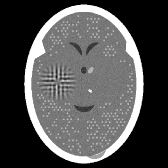
Figure 1: The head phantom. The value of its TV is 984. Its tomographic data was obtained for 60 views.

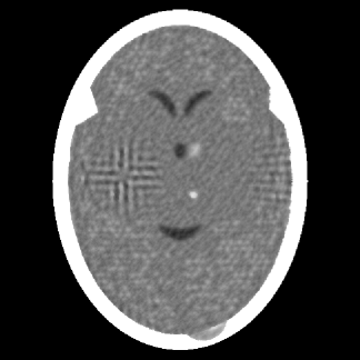
(a)

 

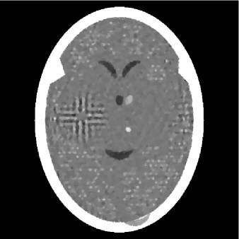
(b)

Figure 2: Reconstructions of the head phantom of Figure 1. (a) The image reconstructed by the PSM has $TV=919$ and was obtained after 2217 seconds. (b) The image reconstructed by the SM has $TV=873$ and was obtained after 102 seconds.

Data were collected by calculating line integrals through the digitized head phantom in Figure 1 using $60$ sets of equally rotated (in $3$ degrees increments) parallel lines, with lines in each set spaced at $0.752$ mm from each other. Each line integral gives rise to a linear equation and represents a hyperplane in $\mathbb{R}^{J}$. The phantom itself lies in the intersection of all the hyperplanes that are associated with these lines, and it also satisfies the box constraints in (10). The total number of linear equations is $18,524$, making our problem underdetermined with $235,225$ unknowns (the intersection of all the hyperplanes is in an at least $216,701$-dimensional subspace of $R^{235,225}$). In the comparative study, we first applied the PSM and then the SM to these data as follows.

The PSM was implemented as described in Subsection 5.2.1. In particular, it started with the zero vector, for which ${Prox}_{C}\left(x^{0}\right)=326$. It was stopped according to the Stopping Rule (P3), the iteration number at that time was 815 and the value of the proximity function was ${Prox}_{C}\left(x^{815}\right)=0.0422$, which is very much smaller than the value at the initial point. The computer time required was 2217 seconds. The TV of the output was 919, which is less than that of the phantom, indicating that the PSM is performing its task of producing a constraints-compatible output with a low TV. This output is shown in Figure 2(a).

We used the Superiorized Version of the Basic Algorithm, as described in Subsection 5.2.2 to generate a sequence $\left\{y^{k}\right\}_{k=0}^{\infty}$ until it reached $O\left(C,0.0422,\left\{y^{k}\right\}_{k=0}^{\infty}\right)$ and considered that to be the output of the SM. We know that this output must exist for our problem and that its constraints-compatibility will not be greater than that of the output of the PSM. The computer time required to obtain this output was 102 seconds, which is over twenty times shorter than what was needed by the PSM to get its output. The TV of the the SM output was 876, which is also less than that of the output of PSM. The SM output is shown in Figure 2(b).

	$TV$ value	Time (seconds)
PSM	919	2217
SM	873	102

Table 1: Performance comparison of the PSM and the SM when producing the reconstructions in Figure 2.

As summarized in Table 1, with the stopping rule that guarantees that the output of the SM is at least as constraints-compatible as the output of the PSM, the SM showed superior efficacy compared to the PSM: it obtained a result with a lower TV value at less than one twentieth of the computational cost.

6 Conclusions

The superiorization methodology (SM) allows the conversion of a feasibility-seeking algorithm, designed to find an $\varepsilon$-compatible solution of the constraints, into a superiorized algorithm that inserts, into the feasibility-seeking algorithm, objective function reduction steps while preserving the guaranteed feasibility-seeking nature of the algorithm. The superiorized algorithm interlaces objective function nonascent steps into the original process in an automatic manner. In case of strong perturbation resilience of the original feasibility-seeking algorithm, mathematical results indicate why the superiorized algorithm will be efficacious for producing an $\varepsilon$-compatible solution output with a low value of the objective function.

We have presented an example for which the SM finds a better solution to a constrained minimization problems than the projected subgradient method (PSM), and in significantly less computation time. This finding is understandable in view of the nature of how the methods interlace feasibility-oriented activities with optimization activities. While the PSM requires a projection onto the feasible region of the constrained minimization problem, the SM needs to do only projections onto the individual constraints whose intersection is the feasible region. We demonstrated this experimentally on a large-sized application that is modeled, and needs to be solved, as a constrained minimization problem.

Acknowledgments. We thank the editor and reviewer for their constructive comments. We would like to acknowledge the generous support by Dr. Ernesto Gomez and Dr. Keith Schubert in allowing us to use the GPU cluster at the Department of Computer Science and Engineering at California State University San Bernardino. We are also grateful to Joanna Klukowska for her advice on using optimized compilation for speeding up SNARK09. This work was supported by the United States-Israel Binational Science Foundation (BSF) Grant No. 200912, the U.S. Department of Defense Prostate Cancer Research Program Award No. W81XWH-12-1-0122, the National Science Foundation Award No. DMS-1114901, the U.S. Department of Army Award No. W81XWH-10-1-0170, and by Grant No. R01EB013118 from the National Institute of Biomedical Imaging and Bioengineering and the National Science Foundation. The contents of this publication is solely the responsibility of the authors and does not necessarily represent the official views of the National Institute of Biomedical Imaging and Bioengineering or the National Institutes of Health.

References

- (1) Ruszczyński, A.: Nonlinear Optimization. Princeton University Press, Princeton, NJ, USA (2006)
- (2) Nesterov, Y.: Introductory Lectures on Convex Optimization. Kluwer Academic Publishers, Boston/Doredrecht/London (2004)
- (3) Shor, N.Z.: Minimization Methods for Non-Differentiable Functions. Springer-Verlag, Berlin, Heidelberg, Germany (1985)
- (4) Poljak, B.T.: A general method of solving extremum problems. Soviet Math. Dokl. 8, 593–597 (1967)
- (5) Polyak, B.T.: Minimization of unsmooth functionals. USSR Comput. Maths. Math. Phys. 9, 14–29 (1969)
- (6) Beck, A., Teboulle, M.: Mirror descent and nonlinear projected subgradient methods for convex optimization. Oper. Res. Lett. 31, 167–175 (2003)
- (7) Butnariu, D., Davidi, R., Herman, G.T., Kazantsev, I.G.: Stable convergence behavior under summable perturbations of a class of projection methods for convex feasibility and optimization problems. IEEE J. Sel. Topics Signal Process. 1, 540–547 (2007)
- (8) Censor, Y., Elfving, T., Herman, G.T.: Averaging strings of sequential iterations for convex feasibility problems. In: D. Butnariu, Y. Censor, S. Reich (eds.) Inherently Parallel Algorithms in Feasibility and Optimization and Their Applications, pp. 101–114. Elsevier Science Publishers, Amsterdam (2001)
- (9) Censor, Y., Segal, A.: On the string averaging method for sparse common fixed point problems. Int. Trans. Oper. Res. 16, 481–494 (2009)
- (10) Censor, Y., Segal, A.: On string-averaging for sparse problems and on the split common fixed point problem. Contemp. Math. 513, 125–142 (2010)
- (11) Censor, Y., Tom, E.: Convergence of string-averaging projection schemes for inconsistent convex feasibility problems. Optim. Methods Softw. 18, 543–554 (2003)
- (12) Penfold, S.N., Schulte, R.W., Censor, Y., Bashkirov, V., McAllister, S., Schubert, K.E., Rosenfeld, A.B.: Block-iterative and string-averaging projection algorithms in proton computed tomography image reconstruction. In: Y. Censor, M. Jiang, G. Wang (eds.) Biomedical Mathematics: Promising Directions in Imaging, Therapy Planning and Inverse Problems, pp. 347–367. Medical Physics Publishing, Madison, WI, USA (2010)
- (13) Censor, Y., Davidi, R., Herman, G.T.: Perturbation resilience and superiorization of iterative algorithms. Inverse Problems 26, 065,008 (2010)
- (14) Davidi, R., Herman, G.T., Censor, Y.: Perturbation-resilient block-iterative projection methods with application to image reconstruction from projections. Int. Trans. Oper. Res. 16, 505–524 (2009)
- (15) Herman, G.T., Davidi, R.: Image reconstruction from a small number of projections. Inverse Problems 24, 045,011 (2008)
- (16) Nikazad, T., Davidi, R., Herman, G.: Accelerated perturbation-resilient block-iterative projection methods with application to image reconstruction. Inverse Problems 28, 035,005 (2012)
- (17) Penfold, S.N., Schulte, R.W., Censor, Y., Rosenfeld, A.B.: Total variation superiorization schemes in proton computed tomography image reconstruction. Med. Phys. 37, 5887–5895 (2010)
- (18) Aharoni, R., Censor, Y.: Block-iterative projection methods for parallel computation of solutions to convex feasibility problems. Linear Algebra Appl. 120, 165–175 (1989)
- (19) Bauschke, H.H., Borwein, J.M.: On projection algorithms for solving convex feasibility problems. SIAM Rev. 38, 367–426 (1996)
- (20) Bauschke, H.H., Combettes, P.L.: Convex Analysis and Monotone Operator Theory in Hilbert Spaces. Springer, New York, NY, USA (2011)
- (21) Censor, Y., Chen, W., Combettes, P.L., Davidi, R., Herman, G.T.: On the effectiveness of projection methods for convex feasibility problems with linear inequality constraints. Comput. Optim. Appl. 51, 1065–1088 (2012)
- (22) Censor, Y., Zenios, S.A.: Parallel Optimization: Theory, Algorithms, and Applications. Oxford University Press, New York, NY, USA (1997)
- (23) Cegielski, A.: Iterative methods for Fixed Point Problems in Hilbert Spaces. Lecture Notes in Mathematics 2057, Springer-Verlag, Berlin, Heidelberg, Germany (2012)
- (24) Herman, G.T., Garduño, E., Davidi, R., Censor, Y.: Superiorization: An optimization heuristic for medical physics. Med. Phys. 39, 5532–5546 (2012)
- (25) Jin, W., Censor, Y., Jiang, M.: A heuristic superiorization-like approach to bioluminescence tomography. In: International Federation for Medical and Biological Engineering (IFMBE) Proceedings, vol. 39, pp. 1026–1029 (2012)
- (26) Luo, S., Zhou, T.: Superiorization of EM algorithm and its application in single-photon emission computed tomography (SPECT). Inverse Problems and Imaging, accepted for publication
- (27) Bauschke, H.H., Koch, V.R.: Projection methods: Swiss army knives for solving feasibility and best approximation problems with halfspaces. In: S. Reich, A. Zaslavski (eds.) Proceedings of the workshop "Infinite Products of Operators and Their Applications", Haifa, 2012, accepted for publication. https://people.ok.ubc.ca/bauschke/Research/c16.pdf (2013)
- (28) Helou Neto, E.S., De Pierro, Á.R.: Incremental subgradients for constrained convex optimization: A unified framework and new methods. SIAM J. Optim. 20, 1547–1572 (2009)
- (29) Helou Neto, E.S., De Pierro, Á.R.: On perturbed steepest descent methods with inexact line search for bilevel convex optimization. Optimization 60, 991–1008 (2011)
- (30) Nedić, A.: Random algorithms for convex minimization problems. Math. Program. Ser. B 129, 225–253 (2011)
- (31) Ram, S.S., Nedić, A., Veeravalli, V.: Incremental stochastic subgradient algorithms for convex optimization. SIAM J. Optim. 20, 691–717 (2009)
- (32) Nurminski, E.: The use of additional diminishing disturbances in Fejer models of iterative algorithms. Comput. Math. Math. Phys. 48, 2154–2161 (2008). Original Russian Text: E.A. Nurminski, published in: Zhurnal Vychislitel’noi Matematiki i Matematicheskoi Fiziki 48 (2008), 2121–2128
- (33) Nurminski, E.A.: Fejer processes with diminishing disturbances. Doklady Mathematics 78, 755–758 (2008). Original Russian text: E.A. Nurminski, published in: Doklady Akademii Nauk 422 (2008), 601–604
- (34) Nurminski, E.A.: Envelope stepsize control for iterative algorithms based on Fejer processes with attractants. Optim. Methods Softw. 25, 97–108 (2010)
- (35) Nurminski, E.A.: Fejer algorithms with an adaptive step. Comput. Math. Math. Phys. 51, 741–750 (2011). Original Russian text: E.A. Nurminski, published in: Zhurnal Vychislitel’noi Matematiki i Matematicheskoi Fiziki 51 (2011), 791–801
- (36) Sidky, E.Y., Kao, C., Pan, X.: Image reconstruction in circular cone-beam computed tomography by constrained, total-variation minimization. Phys. Med. Biol. 53, 4777–4807 (2008)
- (37) Herman, G.T.: Fundamentals of Computerized Tomography: Image Reconstruction from Projections, 2nd edn. Springer (2009)
- (38) Combettes, P.L., Pesquet, J.C.: Image restoration subject to a total variation constraint. IEEE Trans. Image Process. 13, 1213–1222 (2004)
- (39) Nesterov, Y.E.: A method for solving the convex programming problem with convergence rate . Soviet Math. Doklady 27, 372–376 (1983)
- (40) Güler, O.: Complexity of smooth convex programming and its applications. In: P.M. Pardalos (ed.) Complexity of Numerical Optimization, pp. 180–202. World Scientific Publishing Co., Singapore, New Jersey (1993)
- (41) Davidi, R., Herman, G.T., Klukowska, J.: SNARK09: A programming system for the reconstruction of 2D images from 1D projections. http://www.dig.cs.gc.cuny.edu/software/snark09/ (2009)
- (42) Klukowska, J., Davidi, R., Herman, G.T.: SNARK09 - A software package for reconstruction of 2D images from 1D projections. Comput. Methods Programs Biomed. 110, 424–440 (2013)