Scaling Exponent for Incremental Records

Abstract

We investigate records in a growing sequence of identical and independently distributed random variables. The record equals the largest value in the sequence, and our focus is on the increment, defined as the difference between two successive records. We investigate sequences in which all increments decrease monotonically, and find that the fraction $I_{N}$ of sequences that exhibit this property decays algebraically with sequence length $N$, namely $I_{N}\sim N^{-\nu}$ as $N\rightarrow\infty$. We analyze the case where the random variables are drawn from a uniform distribution with compact support, and obtain the exponent $\nu=0.317621\ldots$ using analytic methods. We also study the record distribution and the increment distribution. Whereas the former is a narrow distribution with an exponential tail, the latter is broad and has a power-law tail characterized by the exponent $\nu$. Empirical analysis of records in the sequence of waiting times between successive earthquakes is consistent with the theoretical results.

I Introduction

Records, the largest observed values in a sequence of data points wf ; rse ; eig , have long been a topic of interest — anybody who has watched the Olympics will appreciate that much of the suspense lies in seeing if a new world record will be set. Records are a useful tool for characterization of complex systems jk ; gw , and the study of records and their statistical properties has proved valuable in a wide swathe of disciplines, ranging from climate science rp ; ekbhs ; nmt ; wzxw and hydrology vzm to economics ekm ; syn ; bp .

Recent investigations concerning the statistical mechanics of records fwk ; wbk ; ss ; wms reveal rich and interesting phenomenology associated with the effects of round-off errors on record statistics wvrk ; ekmb as well as first-passage behavior sr ; bms of record sequences bk . Here, we introduce a first-passage characteristic that probes how records improve with time, and demonstrate its usefulness for analysis of empirical data.

Tracking an observable over time, one sees the generation of a sequence of records, each new record improving upon the previous one by some finite amount. Intuitively, we expect these improvements to diminish with each new record: the larger the current record is, the less likely it is that the next record improves upon it by a large amount. In this study we ask: how likely we are to see only shrinking improvements over previous records?

Figure 1: Illustration of a sequence with monotonically diminishing increments between records. Records are indicated by filled circles, and the rest of the variables, by open circles. The vertical arrows to the left of a record indicate the magnitudes of the respective increment.

Consider an evolving sequence of $N$ identical and independently distributed random variables. The first element of this sequence is, by definition, a record. Each subsequent element is a record if it is greater than the previous record. Moreover, a new record improves upon the existing one by some increment, defined as the difference between the two records. We study the probability $I_{N}$ that all increments decrease monotonically (see Fig. 1), and our main result is the scaling law

$$I_{N}\sim N^{-\nu}$$ (1)

which holds in the large-$N$ limit. When the random variables are drawn from a compact, uniform distribution, we obtain analytically the exponent

$$\nu=0.317621\ldots.$$ (2)

Our definition of incremental records involves the current record and the previous record, or alternatively, the current record and the current increment. Consequently, the theoretical analysis requires the joint distribution of these two variables. Interestingly, the record and the increment become uncorrelated in the large-$N$ limit, such that the joint distribution is a product of the record distribution and the increment distribution. The former distribution is exponential, but the latter is broad and has power-law tail.

The rest of this paper is organized as follows. In section II, we examine the record distribution, and show that it is the same regardless of whether one considers the set of all records sequences or just the subset of incremental ones. Next, we study the increment distribution which in turn requires the full joint distribution of records and increments (section III). We obtain the increment distribution in the scaling limit, and derive the scaling exponent $\nu$ as a byproduct. In Section IV, we measure the fraction of incremental records for the sequence of waiting times between large earthquakes, and observe good agreement with the theoretical results. We conclude in Section V.

II Record Distribution

Let us consider a sequence of uncorrelated random variables,

$$\{X_{1},X_{2},\ldots,X_{N}\}.$$ (3)

Each variable $X_{i}\geq 0$ is independently drawn from the probability distribution function $\rho(X)$, with the normalization $\int_{0}^{\infty}dX\rho(X)=1$. In many applications, including the earthquake example discussed in section IV, new variables are constantly added to the dataset. Hence, we may view the sequence (3) as evolving with the variable $N$ playing the role of time krb .

The record $x_{i}$ equals the largest variable in a sub-sequence of length $i$. A newly added variable sets a record if it is larger than the previous record,

$$x_{N+1}=\begin{cases}x_{N}&\quad x_{N}\geq X_{N+1},\\ X_{N+1}&\quad X_{N+1}>x_{N},\end{cases}$$ (4)

for $N\geq 1$ with $x_{0}=0$. The first variable necessarily sets a record, $x_{1}=X_{1}$, and by definition, the records increase monotonically, $x_{N+1}\geq x_{N}$.

We focus on the simplest case of a uniform distribution with support in a finite interval, taken without loss of generality as the unit interval,

$$\rho(X)=\begin{cases}1&\quad 0\leq X\leq 1,\\ 0&\quad 1<X.\end{cases}$$ (5)

This distribution is relevant for waiting times between successive earthquakes (see section IV).

The cumulative record distribution $R_{N}(x)$ equals the probability that the record $x_{N}$ is smaller than $x$. This distribution is simply

$$R_{N}(x)=x^{N}.$$ (6)

Indeed, by substituting (5) into $R_{1}(x)=\int_{0}^{x}dX\,\rho(X)$ we have $R_{1}(x)=x$, and further, for the $N$th record to be smaller than $x$, all $N$ variables must be smaller than $x$.

Since the variables are identical and independently distributed, every one of the $N$ variables is equally likely to be the largest. Hence, the probability that the $N$th variable sets a record equals $\frac{1}{N}$, and consequently, the average number of records equals the harmonic number $1+\frac{1}{2}+\frac{1}{3}+\cdots+\frac{1}{N}$. The slow logarithmic growth of this sum demonstrates that when $N$ becomes large, new records are few and far between gkp ; bhi ; gl .

Further, we expect that the improvements made with each new record diminish with time. The increment, defined as the difference between the new record and the old record, quantifies such improvements. Together with the current record $x_{N}$ we also track the current increment $y_{N}$ defined by

$$y_{N+1}=\begin{cases}y_{N}&\quad x_{N+1}=x_{N},\\ x_{N+1}-x_{N}&\quad x_{N+1}>x_{N},\end{cases}$$ (7)

for $N\geq 1$. Again, $y_{1}=x_{1}$ since the first variable is a record.

In this study, we restrict our attention to the subset of sequences where all increments decrease monotonically,

$$y_{1}\geq y_{2}\geq y_{3}\geq\cdots\geq y_{N}.$$ (8)

If this inequality holds, the sequence of records $\{X_{1},X_{2},\ldots,X_{N}\}$ is said to be incremental. We are interested in the probability $I_{N}$ that a record sequence of length $N$ is incremental. Essentially, we require that the quantity $y_{N}-y_{N+1}$ remains non-negative. In this sense, the condition (8) defines a first-passage process, and the quantity $I_{N}$ is analogous to a survival probability sr .

As a preliminary step, we analyze the distribution of incremental records. Specifically, we define the cumulative density $F_{N}(x)$ as the fraction of sequences that: (i) have incremental records, namely, satisfy the condition (8), and (ii) have a record smaller than $x$, that is, $x_{n}<x$. Of course, $I_{N}\equiv F_{N}(x=1)$.

Figure 2: Geometric representation of incremental sequences of length two. The shaded area represents sequences $\{X_{1},X_{2}\}$ with incremental records and current record $x_{2}<x$.

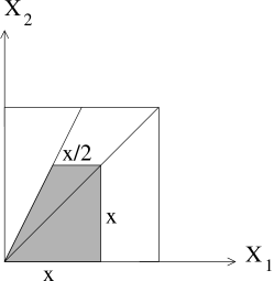
When $N=1$, we have $F_{1}(x)=R_{1}(x)$ and hence, $I_{1}=1$. When $N=2$, the two-variable sequence $\{X_{1},X_{2}\}$ corresponds to a point inside the unit square (figure 2). If $X_{1}>X_{2}$, the record sequence is necessarily incremental. Otherwise, the sequence is incremental if and only if $X_{2}-X_{1}\leq X_{1}$. Accordingly, the lines $X_{2}=X_{1}$ and $X_{2}=2X_{1}$ divide the unit square into three triangles, in two of which the condition (8) holds. To obtain the probability $F_{2}(x)$ that an incremental sequence has record $x_{2}\leq x$, we overlay a square of area $x^{2}$ onto the unit square. The overlap between this square and the two relevant triangles is a trapezoid with height $x$, and bases $x$ and $x/2$ (figure 2). The area of this trapezoid gives the cumulative record density

$$F_{2}(x)=\frac{3}{4}\,x^{2},$$ (9)

and hence, $I_{2}=\tfrac{3}{4}$.

This illuminating example suggests that generally,

$$F_{N}(x)=I_{N}\,x^{N}.$$ (10)

Indeed, when $N=3$, in addition to the planes $X_{2}=X_{1}$, $X_{2}=2X_{1}$, and similarly, $X_{3}=X_{1}$ and $X_{3}=2X_{1}$, there is a fifth plane $X_{3}-X_{2}=X_{2}-X_{1}$ that corresponds to three distinct records. These planes specify a polyhedron with volume $F_{3}(x)=\tfrac{47}{72}\,x^{3}$, embedded inside a cube of volume $x^{3}$; The condition (8) holds inside this polyhedron. In general, the hyperplanes defined by (8) are invariant under the transformation $X_{i}\to aX_{i}$. Consequently, the cumulative distribution equals the volume of an $N$-dimensional polyhedron, embedded in an $N$-dimensional hypercube of volume $x^{N}$. This geometric argument and the normalization $F_{N}(1)=I_{N}$ support equation (10) (numerical confirmation is shown in figure 3). Remarkably, the normalized distribution function $F_{N}(x)/F_{N}(1)$ is identical to $R_{N}(x)$ given in (6). Hence, records in incremental sequences and records in all sequences are characterized by identical distribution functions.

Figure 3: The normalized cumulative distribution $F_{N}(x)/F_{N}(1)$ for $N\leq 4$. The circles represents results of Monte Carlo simulations and the lines show the corresponding monomials $x^{N}$.

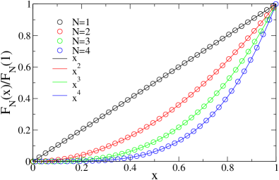
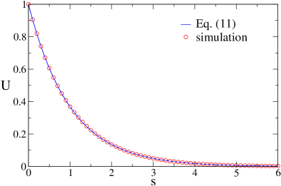
Our main focus is the asymptotic behavior in the limit $N\to\infty$ where the cumulative density (10) follows the scaling form (figure 4)

$$F_{N}(x)\simeq I_{N}\,e^{-s},\qquad s=(1-x)N.$$ (11)

To obtain this form, we simply rewrite $x^{N}=[1-(1-x)]^{N}$ and consider the limits $N\to\infty$ and $x\to 1$ with the scaling variable $s=(1-x)N$ being finite. Thus, the term $x^{N}$ implies that the record distribution is exponential ft ; eig1 .

Figure 4: The scaling function governing the records. The circles represent results of Monte Carlo simulations for the fraction $U(s)$ of incremental sequences with scaled record $(1-x)N$ that is larger than $s$. Also shown for reference is the prediction $U(s)=\exp(-s)$ that follows from Eq. (11).

III Increment Distribution

As evident from the definitions (4) and (7), the increment is coupled to the record. Hence, further analysis requires the joint record-increment distribution. We study the probability density $S_{N}(x,y)$, defined such that $S_{N}(x,y)\,dx\,dy$ is the probability that the record $x_{N}$ lies in the infinitesimal range $(x,x+dx)$ and similarly, the increment $y_{N}$ is in the range $(y,y+dx)$. Since $y<x$, the fraction of incremental sequences is the following integral of the joint density,

$$I_{N}=\int_{0}^{1}dx\int_{0}^{x}dy\,S_{N}(x,y).$$ (12)

The probability density satisfies the recursion equation

$$S_{N+1}(x,y)=x\,S_{N}(x,y)+\int_{y}^{x-y}dy^{\prime}\,S_{N}(x-y,y^{\prime})$$ (13)

for $N>1$, with $S_{1}(x,y)=\delta(x-y)$ as the first element is necessarily a record. The first term on the right-hand side of (13) accounts for cases where the old record holds. The integral term accounts for situations where the old record, which necessarily equals $x-y$, is surpassed by a new record; The lower integration limit enforces the monotonicity condition (8). Starting with $S_{1}(x,y)=\delta(x-y)$ we find $S_{2}(x,y)=x\delta(x-y)+\Theta(x-2y)$ from which $I_{2}=3/4$ is recovered.

To study the asymptotic behavior for large $N$, we convert the recursion equation (13) into the integro-differential equation

$$\frac{\partial S_{N}(x,y)}{\partial N}=-(1-x)S_{N}(x,y)+\int_{y}^{x-y}dy^{\prime}\,S_{N}(x-y,y^{\prime}).$$ (14)

To obtain this equation, we subtract $S_{N}(x,y)$ from both sides of (13) and then replace the difference $S_{N+1}-S_{N}$ with the derivative $\partial S_{N}/\partial N$.

The scaling behavior (11) shows that $1-x\sim N^{-1}$. Moreover, the integral term in (14) implies that, similarly, the increment is inversely proportional to sequence length, $y\sim N^{-1}$. Hence, we anticipate the scaling form

$$S_{N}(x,y)\simeq I_{N}\,N^{2}\,\Psi(s,z),\qquad z=y\,N.$$ (15)

The normalization (12) sets the prefactor $I_{N}\,N^{2}$ and implies that the scaling function $\Psi(s,z)$ is normalized, $\int_{0}^{\infty}\int_{0}^{\infty}ds\,dz\,\Psi(s,z)=1$. If we integrate the joint scaling function over the scaled increment, we should recover the distribution of the scaled record, given in (11),

$$\int_{0}^{\infty}dz\,\Psi(s,z)=e^{-s}.$$ (16)

Figure 5: The fraction of incremental sequences versus sequence length. The quantity $I_{N}$, measured from Monte Carlo simulations is compared with the theoretical result (1)-(2). The numerical results are obtained from $10^{8}$ independent realizations.

Next, we substitute (15) along with $I_{N}\simeq A\,N^{-\nu}$ as in (1) into the evolution equation (14), and find that the scaling function satisfies

$$\left(\!2\!-\!\nu\!+\!s\!+\!s\frac{\partial}{\partial s}\!+\!z\frac{\partial}{\partial z}\!\right)\!\Psi(s,z\!)=\!\int_{z}^{\infty}\!\!dz^{\prime}\Psi(s+z,z^{\prime}).$$ (17)

Remarkably, this rather involved integro-differential equation admits a separation-of-variables solution

$$\Psi(s,z)=e^{-s}\,\phi(z).$$ (18)

This form is consistent with Eq. (16) when the scaling function $\phi(z)$ that characterizes the distribution of increments, is normalized, $\int_{0}^{\infty}dz\,\phi(z)=1$. The factorizing form (17) implies that records and increments become uncorrelated in the limit $N\to\infty$, an assumption that is supported by the numerical simulations (see below).

Figure 6: The cumulative distribution of increments. Shown is the probability $\Phi(z)$ that the scaled increment $yN$ is larger than the scaling variable $z$. The simulation results were obtained by generating $10^{7}$ independent increments for a sequence of length $N=10^{6}$. The theoretical result represents a numerical solution of (20) with $\nu$ given by Eq.(2).

By substituting the factorizing form (18) into the governing equation (17), we obtain the integro-differential equation

$$z\frac{d\phi(z)}{dz}+(2-\nu)\phi(z)=e^{-z}\int_{z}^{\infty}\phi(z^{\prime})dz^{\prime}.$$ (19)

We can convert this first-order equation for $\phi(z)$ into a second order ordinary differential equation for its integral, $\Phi(z)=\int_{z}^{\infty}dz^{\prime}\,\phi(z^{\prime})$,

$$z\frac{d^{2}\Phi(z)}{dz^{2}}+(2-\nu)\frac{d\Phi(z)}{dz}+e^{-z}\Phi(z)=0.$$ (20)

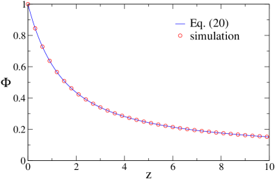
The two boundary conditions are $\Phi(0)=1$ and $\Phi^{\prime}(0)=-1/(2-\nu)$. The former follows from the fact that $\phi(z)$ is normalized, and the second boundary condition follows from equation (19) itself.

Equation (20) has two independent solutions. In the large-$z$ limit, the rightmost term in Eq. (20) vanishes, and consequently, one of these solution approaches a constant, $\Phi(z)\to C$, while the other decays algebraically,

$$\Phi(z)\sim z^{\nu-1}.$$ (21)

This former solution is not physical because the scaling function $\phi(z)$ vanishes in the limit $z\to\infty$. The exponent $\nu$ plays the role of an “eigenvalue” of equation (20). Numerically, we integrate (20) with a trial value $\nu_{\rm try}$. When $\nu_{try}\neq\nu$, the solution approaches a nonzero constant $C\equiv C(\nu_{\rm try})\neq 0$ when $z\to\infty$. Only when $\nu_{\rm try}$ equals the eigenvalue $\nu$, does this constant vanish $C(\nu)=0$, and the physical solution (21) is realized. We used the Adams method ba to perform the numerical integration and the bisection method nr to find the root of the equation $C(\nu)=0$. The result $\nu=0.31762101\ldots$ quoted in (2) follows.

Equation (21) implies that the increment distribution decays algebraically for sufficiently large increments. Let $P_{N}(y)dy$ be the probability that an incremental sequence has latest increment in the range $(y,y+dy)$. The probability density $P_{N}(y)$ follows from the joint density,

$$P_{N}(y)=\int_{y}^{1}dx\,S_{N}(x,y).$$ (22)

By substituting the scaling behavior (15) with the factorizing form (18) into the integral, we find that the increment density has the scaling form

$$P_{N}(y)\simeq I_{N}\,N\,\phi(z).$$ (23)

The scaling function $\phi(z)$ is simply $\phi(z)=-\Phi^{\prime}(z)$. Therefore, using the algebraic tail (21), we find $\phi(z)\sim z^{\nu-2}$. Hence, the increment density decays algebraically,

$$P_{N}(y)\sim N^{-1}y^{\nu-2},$$ (24)

for sufficiently large increments $y\gg N^{-1}$.

The algebraic decay (24) matches our expectation that is based on a simple heuristic argument. The probability that the first element is largest equals $N^{-1}$. Since a sequence with only one record is incremental, we expect that $P_{N}(1)\sim N^{-1}$. This behavior agrees with (24). Hence, from the extreme case of a single record that is nearly maximal, $y\approx 1$, we can derive the algebraic behavior (24) from the scaling behavior (23) together with (1). We note that the same argument applies to all record sequences. This heuristic argument, combined with the fact that $F_{N}(x=1)\equiv 1$, yields $P_{N}(y)\sim N^{-1}y^{-2}$ for all record sequences.

We performed numerical simulations to test the above predictions. In each simulation run, the initial record and the initial increment are respectively set as $x_{0}=0$ and $y_{0}=1$. Then at each step a random number in the range $[0:1]$ is drawn nr . The record and the increment are calculated from (4) and (7) respectively. This elementary step is iterated as long as the monotonicity condition $y_{N+1}\leq y_{N}$ is satisfied, but the run is aborted when this condition is violated for the first time. For example, the quantity $I_{N}$ is measured as the fraction of such runs where at least $N+1$ random numbers where generated.

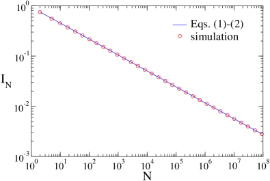
Results of these Monte Carlo simulations confirm the theoretical prediction. First, as shown in figure 5, the fraction of incremental sequences decays algebraically as in equations (1)-(2). Second, as shown in figure 6, the probability $\Phi(z)$ that the scaled increment $yN$ is larger than $z$ agrees with the predictions of equation (20), with the exponent $\nu$ specified in (2). Finally, we also confirmed directly that the record and the increment become uncorrelated, that is, $\langle(1-x)y\rangle/\langle 1-x\rangle\langle y\rangle\to 1$ when $N\to\infty$.

Figure 7: The probability $I_{N}$ as calculated using data for earthquakes of magnitude $4$ and above. The empirical results are compared with theoretical predictions for the compact, uniform distribution.

IV Empirical Study

Records are a basic feature of a data set, as for example, the record high and record low specify the span of the set. It is natural to ask whether the statistical measures introduced in this study are useful as a data analysis tool. We believe that the notion of incremental records is a sensible measure of performance bk , especially since it involves no prior knowledge of how the random variables are distributed. Also, determining whether a sequence includes only incremental records is straightforward. There is a difficulty, however. In practice, a very large number of data points is required to accurately measure the fraction $I_{N}$ because this survival probability decays as a power-law.

Here, we analyze inter-event times between successive earthquakes. In ref. bk , it was demonstrated that the average number of records in inter-event times is a straightforward test for whether powerful earthquakes occur randomly in time and follow Poisson statistics am ; st ; bdj . Inter-event times are not bounded from above, but they are bounded from below, by zero. Given that our theoretical analysis applies to bounded random variables, rather than studying increments in the record high, we studied decrements in the record low. As the transformation $X_{N}\to 1-X_{N}$ shows, the behavior (1)-(2) also characterizes decrements in record lows.

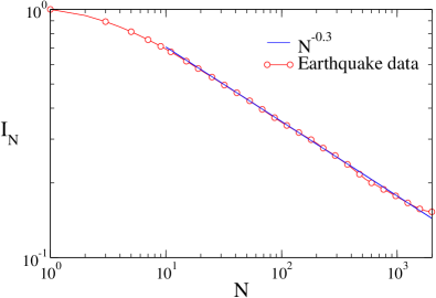
Our dataset lists the event times for the $\approx 189,000$ earthquakes with magnitude $M>4$ gr that occurred worldwide during the years $1984-2012$ data . From these event times, the sequence (3) of inter-event times is constructed as a list of the waiting times between consecutive earthquakes (zero waiting times are ignored). Our procedure for determining $I_{N}$ from this data set is to treat $N$ consecutive data points as an independent sequence, and then calculate the fraction of these which have only incremental records. That is to say, when calculating $I_{1}$ we consider each individual element of the full data set to be a sequence of length $1$, when calculating $I_{2}$ each consecutive pair of events to be a distinct sequence of length $2$, and so forth.

As Fig. 7 shows, we observe scaling behavior which closely matches the theoretical predictions (1)-(2). The measured exponent is remarkably close to the theoretical value

$$\nu_{\rm data}=0.30\pm 0.03.$$ (25)

As discussed in the conclusions, the tail of the distribution function from which the random variables are drawn controls $\nu$ bk . Hence, the empirical data combined with the theoretical results above suggests that there are no singularities (due to aftershocks) in the distribution of inter-event times, $\lim_{X\to 0}\rho(X)={\rm const}$. Moreover, the empirical results show that the fraction of incremental records is a sensible quantity in the context of data analysis, and provide an example where the fraction $I_{N}$ decays algebraically.

Figure 8: The exponent $\nu$ versus the parameter $\mu$ characterizing the parent distribution $\rho(X)$ in (26).

V Conclusions

In conclusion, we studied the probability that all records in a sequence of random variables are incremental. In our definition, a record is incremental if it improves upon the previous record by a yet smaller amount. We found two scaling laws: one for the probability that a sequence is incremental, and one for the distribution of increments. A single scaling exponent underlies both of these scaling laws. Interestingly, even for the simplest case of identical and independently distributed random variables, drawn from a uniform distribution, this scaling exponent is nontrivial. Using an empirical analysis of earthquake data, we demonstrated that statistics of incremental records are a sensible tool for data analysis.

Our theoretical analysis involved the joint distribution of record value and increment size. Initially, these two variables are perfectly correlated, but as the sequence grows, the correlation between these two variables diminishes, and it eventually vanishes. This key observation allows us to solve for the full distribution of records and increments in the scaling limit and obtain as a byproduct the scaling exponent.

Our study concerns an ensemble of sequences for which improvements in records diminish steadily with time. It is useful to compare statistical properties of records and increments for this restricted ensemble of sequences with the corresponding behavior for the full ensemble of sequences krb . Our findings show that the most basic characteristic, the record, does not distinguish between these two ensembles, yet, differences in the record are a more sensitive measure whose distribution does differentiate between the two.

In a recent related study, it was shown that another measure for performance, the probability that records always remain above their expected average, is also characterized by a nontrivial scaling exponent bk . Taken together, these two closely related studies indicate that there is a family of first-passage exponents bk1 that characterize extreme statistics.

An interesting challenge is to generalize the above results to arbitrary distributions, both compact and noncompact. Numerically, we also studied the general class of compact distribution functions with algebraic tail

$$\rho(X)=\begin{cases}\mu(1-X)^{\mu-1}&\quad 0\leq X\leq 1,\\ 0&\quad 1<X,\end{cases}$$ (26)

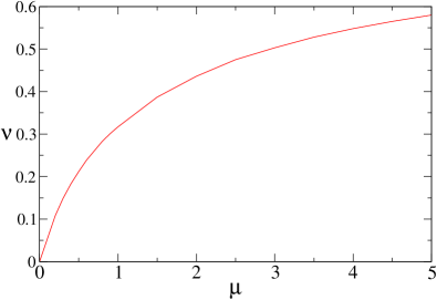
for $0\leq X\leq 1$. The simulations show that the exponent $\nu$ varies continuously with the parameter $\mu$ (figure 8). Qualitatively, this behavior is in line with the results of several other studies showing that the tail of the distribution $\rho$ governs scaling laws for extreme statistics bk ; bkr ; kj . It will be interesting to establish whether the increment and the record decouple in general, and to obtain the scaling exponent $\nu$ using analytic methods.