Patience-aware Scheduling for Cloud Services:
Freeing Users from the Chains of Boredom

Abstract

Scheduling of service requests in Cloud computing has traditionally focused on the reduction of pre-service wait, generally termed as waiting time. Under certain conditions such as peak load, however, it is not always possible to give reasonable response times to all users. This work explores the fact that different users may have their own levels of tolerance or patience with response delays. We introduce scheduling strategies that produce better assignment plans by prioritising requests from users who expect to receive the results earlier and by postponing servicing jobs from those who are more tolerant to response delays. Our analytical results show that the behaviour of users’ patience plays a key role in the evaluation of scheduling techniques, and our computational evaluation demonstrates that, under peak load, the new algorithms typically provide better user experience than the traditional FIFO strategy.

1 Introduction

Job schedulers are key components of Clouds as they are responsible not only for assigning user tasks to resources but also for notifying management systems on when resources need to be allocated or released. These resource allocation decisions, specially on when to allocate additional resources, have an impact on both provider costs and user experience, and are particularly relevant to manage resources under peak loads.

Traditionally, job schedulers do not take into account how users interact with services. They optimise system metrics, such as resource utilisation and energy consumption, and user metrics such as response time. However, understanding interactions between users and a service provider over time allows for custom optimisations that bring benefits for both parties. Such interactions are becoming more pervasive due to the large number of users accessing Cloud services via mobile devices and analytics applications that require multiple service requests.

In this article we propose scheduling strategies that take into account users’ expectations regarding response time and their patience when interacting with Cloud services. Such strategies are relevant mainly to handle peak load conditions without the need to allocate additional resources for the service provider. Although elasticity is common in a Cloud setting, resources may not be available quickly enough and their allocation can incur additional costs that may be avoidable. The main contributions of this paper are:

• The introduction of a Patience-Aware Scheduling (PAS) strategy and an Expectation-Aware Scheduling (EAS) strategy for Cloud systems;

• Analytical comparisons between the EAS strategy and the traditional First-In, First-Out (FIFO) scheduling strategy;

• Evaluation of the proposed strategies and a detailed discussion on when they bring benefits for users and service providers.

2 Proposed Scheduling Strategies

This section describes the proposed strategies, PAS and EAS, and presents several analytical results that compare EAS with FIFO. We chose FIFO for comparison because it is one of the most used scheduling techniques that explores fairness of users by scheduling requests as they arrive in the system.

2.1 Common Characteristics Shared by PAS and EAS

This work considers Cloud services (e.g. data analytics, Web search, social networks) that back applications running on mobile devices and desktops, most of which are highly interactive and iterative. Users, consciously or not, interact with a service provider multiple times when using their applications. Service performance over time usually shapes the users’ expectations on how it is likely to perform in the future. The service provider stores information on how its service responded to user requests and uses this information to gauge her expectations and patience.

PAS and EAS utilise user expectation to schedule service requests on the Cloud’s resources. Both strategies share the following common goals:

• Minimise the number of users abandoning the service;

• Maximise the users’ level of happiness with the service;

• Perform such optimisations without adding new resources to the service.

We remark that an incoming job request will be directly assigned if there are available resources in the service provider. Therefore, choosing among FIFO, PAS, and EAS becomes more crucial during peak load.

2.2 Patience-aware Scheduling

PAS has the goal of serving first users whose patience levels are the lowest when interacting with the Cloud service. When new requests arrive, the algorithm sorts the tasks in its waiting queue according to the Patience of their users (in ascending order), and when a new resource is freed, the request positioned in the head of the waiting list is assigned to it.

An adequate estimate of how the user’s happiness level and the user’s tolerance curves behave is very important for the evaluation of the proposed strategies. In our implementation of PAS and in our computational evaluation, we employed the definition of user’s patience suggested by Brown et al. [6]. Patience is hence given by the ratio of the time a user expects to wait for results to the time the user actually waits for them:

$$\text{Patience}=\frac{\text{Expected Response Time}}{\text{Actual Response Time}}$$

2.3 Expectation-aware Scheduling

EAS has the goal of serving first requests associated to users whose response time expectations are translated into “soft” deadlines that are positioned earlier in time. The difference between EAS and traditional deadline-based algorithms lies in the nature of the “buffer” adding to the minimum response time, as it changes over time and is related to users’ patience.

EAS sorts service requests in the waiting queue according to their users’ expectation, given by:

$$\text{Expectation}=\text{arrival time}+\text{expected response time},$$

where arrival time is the time at which the job arrived on the waiting queue and expected response time is the time that the service provider need to complete the task. EAS, then, schedules the job with the least expectation when a new resource is freed.

2.4 Analytical Investigation of the EAS Strategy

In this section, we analyse EAS from a theoretical point of view by comparing it with FIFO. The notation used throughout this section is presented in Table 1 and explained in more details in the section below.

2.4.1 Notation.

Table 1: List of symbols.

$\mathcal{T}$	sequence of arriving tasks
$t$	task in $\mathcal{T}$
$a(t)$	arrival time of task $t$
$s(t)$	time at which task $t$ starts to be processed
$r(t)$	response time for $t$
$\mathcal{U}$	set of users
$u$	user in $\mathcal{U}$
$e(u,t)$	time difference between user $u$’s expectation and real response time
$\Delta(t)$	processing time of task $t$
$u(t)$	user that submitted task $t$
$w(u)$	time tolerance that $u$ has for the results of some service
$m$	parallelism capacity of service provider
$h(u)$	user $u$’s level of happiness with service provider
$c(u)$	minimum level of happiness at which user $u$ still uses a service
$i(u,e(u,t))$	variation of $h(u)$ according to $e(u,t)$
$j(u,t,e(u,t))$	variation of $w(u,t)$ according to $e(u,t)$
$Z$	closed interval $[0,1]\in\mathbb{R}$
$Z^{|\mathcal{U}|}$	user happiness state space

Let $\mathcal{U}$ be the set of users of a service provider. Let $\mathcal{T}$ denote the sequence of job requests being submitted, where each $t\in\mathcal{T}$ arrives at time $a(t)\in\mathbb{R}^{+}$ and has processing time $\Delta(t)\in\mathbb{R}$. Task $t$ is submitted by user $u(t)$, who is expecting to wait an amount of time $w(u(t))\in\mathbb{N}$ in addition to $\Delta(t)$, i.e., $w(u)$ denotes $u$’s tolerance with response delays. The service provider has a dispatching algorithm responsible for the assignment of each incoming task to one of its $m$ indistinguishable and non-preemptive processors.

Let us denote by $s(t)\in\mathbb{R}^{+}$ the time at which task $t$ starts to be processed. The response time for task $t$ is given by $r(t)=(s(t)-a(t))+\Delta(t)$, and $e(u(t),t)=r(t)-(\Delta(t)+w(u(t)))$ denotes the amount of time by which the response time differs from $u(t)$’s original expectation.

We denote user $u$’s level of happiness by $h(u)\in\left[0,1\right]$, a linear scale where $h(u)=0$ and $h(u)=1$ indicates that $u$ is absolutely discontent and happy, respectively. We assume that $u$ stops sending requests as soon as $h(u)$ reaches a value below some critical value $c(u)$ in $\left[0,1\right]$. We say that user $u$ is active if $h(u)>c(u)$. The impact that $e(u,t)$ has on $h(u)$ is formulated by function $i:\mathcal{U}\times\mathbb{R}\rightarrow\mathbb{R}$, and the impact that $e(u,t)$ has on $w(u)$ is described by some function $j:\mathcal{U}\times\mathcal{T}\times\mathbb{R}\rightarrow\mathbb{R}$. If we assume that $i(u,e(u,t))$ and $j(u,t,e(u,t))$ are addictive factors, then, after the computation of some task $t$, the happiness level of user $u(t)$ will be given by $h(u)+i(u,e(u,t))$, while $u(t)$’s patience level becomes $w(u(t))+j(u(t),t,e(u(t),t))$.

2.4.2 Optimisation Criteria.

Let $Z$ denote the closed interval $[0,1]\subset\mathbb{R}$. We say that a vector $s\in Z^{|\mathcal{U}|}$ denotes a service provider’s user happiness state if $s_{x}=h(u_{x})$ $\forall u_{x}\in\mathcal{U}$, $1\leq x\leq\mathcal{U}$. In order to evaluate and compare different scheduling strategies, we have to define a cost function $c:Z^{|\mathcal{U}|}\rightarrow\mathbb{R}$. It is clear that the definition of a proper cost function depends on the optimisation criteria one wants to establish.

For our theoretical analysis, we will consider two optimisation goals. The first one is the maximisation of the overall happiness of users, where service providers should try to reach states $s\in Z^{|\mathcal{U}|}$ of maximal $L^{1}$-norm. The other criteria consists of the maximisation of active users, where service providers try to keep as many active users as possible. Formally, a state $s\in Z^{|\mathcal{U}|}$ satisfying this second goal is associated to a vector $s^{\prime}\in Z^{|\mathcal{U}|}$ such that $s^{\prime}_{x}=s_{x}$ if $s_{x}\geq c(u_{x})$, $s^{\prime}_{x}=0$ otherwise, and $||s^{\prime}||_{0}$ is maximal.

In the following sections, we investigate two scenarios for the problem and discuss the situations where these different optimisation criteria may be employed and how the proper choice of a scheduling algorithm depends strongly on the behaviour of functions $i$ and $j$.

2.4.3 Batch Requests.

We consider initially how scheduling strategies affect the user happiness states when we take into account a single batch of job requests. We assume here that each user submits a single request, and therefore we do not investigate variations of $w(u)$. Single batch analysis is interesting because it is the only reasonable option when requests do not arrive in a periodic fashion and users’ profiles are unknown, i.e., when we do not have an exact idea about their patiences’ levels and behaviours. The optimisation criteria in this section will be the $L^{1}$-norm of the user happiness state vector.

Let us consider the family of scenarios where each task in $\mathcal{T}$ consumes time $\Delta$, and let $t_{x},t_{y}\in\mathcal{T}$ be such that $x+m<y$ and $a(t_{x})+w(u_{x})>a(t_{y})+w(u_{y})$.

If FIFO is employed, the scheduling plan $P$ will have each request $t$ serviced according to the order defined by its arriving time $a(t)$. In particular, $t_{x}$ will be processed before $t_{y}$ according to $P$ and in different moments in time (i.e., they will not be serviced in parallel).

For the same sequence $\mathcal{T}$, because $a(t_{x})+w(u_{x})>a(t_{y})+w(u_{y})$, EAS would invert the order in which tasks $t_{x}$ and $t_{y}$ are processed, so let us consider the plan $P^{\prime}$ that is almost equal to $P$, having only the positions of $t_{x}$ and $t_{y}$ exchanged. Because all the tasks consume the same amount of time, it is clear that we can transform plan $P$ into plan $P^{*}$ that would be generated by EAS if we apply the same exchange technique sequentially until every pair of requests is positioned accordingly.

Let $s$ and $s^{\prime}$ be the user happiness state vectors of $p$ after the execution of plans $P$ and $P^{\prime}$, respectively, and let $f_{x}$ and $f_{y}$ be the times at which $t_{x}$ and $t_{y}$ have their processing tasks finished according to plan $P$, respectively (i.e., $f_{x}<f_{y}$). Let us refer to $e(t_{x})$ and $e(t_{y})$ as $e^{1}(t_{x})$ and $e^{1}(t_{y})$ for FIFO, respectively, and as $e^{2}(t_{x})$ and $e^{2}(t_{y})$ for EAS, respectively.

Finally, let $q_{x,y}:\mathbb{R}\times\mathbb{R}\rightarrow\mathbb{R}$ be the function parameterized by $e(t_{x})$ and $e(t_{y})$ denoting the sum of the changes in the happiness levels of users $u_{x}$ and $u_{y}$ after tasks $t_{x}$ and $t_{y}$ have been serviced, respectively. It is clear that $q_{x,y}$ depends on the behaviour of $i$.

Proposition 1

If $q_{x,y}$ is always the same $\forall x,y\in\mathcal{U}$, is monotonic, and respects exactly one of the following scenarios, then it is possible to decide if either EAS or FIFO yields a plan resulting in a user happiness state $s$ with maximal $||s||_{1}$:

• $f_{x,y}(a,b)\geq f_{x,y}(c,d)$ whenever $|a|+|b|\geq|c|+|d|$; or

• $f_{x,y}(a,b)\leq f_{x,y}(c,d)$ whenever $|a|+|b|\geq|c|+|d|$; or

• $f_{x,y}(a,b)=f_{x,y}(c,d)$ whenever $|a|+|b|\geq|c|+|d|$.

Proof

Simple inspection shows that $a(t_{x})+\Delta+w(u_{x})$, $a(t_{y})+\Delta+w(u_{y})$, $f_{x}$, and $f_{y}$ can appear in six different relative ordering schemes (e.g., $a_{y}+\Delta+w(u_{y})<a_{x}+\Delta+w(u_{x})<f_{x}<f_{y}$ is one of them). Moreover, one can also see that $e^{1}(t_{x})+e^{1}(t_{y})=e^{2}(t_{x})+e^{2}(t_{y})$ and that $max(e^{1}(t_{x}),e^{1}(t_{y}))>max(e^{2}(t_{x}),e^{2}(t_{y}))$ in each of these cases. Therefore, we have $|e^{1}(t_{x})|+|e^{1}(t_{y})|\geq|e^{2}(t_{x})|+|e^{2}(t_{y})|$.

Based on these observations and on our hypothesis, we have the following situations:

• if $f_{x,y}(a,b)\geq f_{x,y}(c,d)$ whenever $|a|+|b|\geq|c|+|d|$, then $c(s)\geq c(s^{\prime})$;

• if $f_{x,y}(a,b)\leq f_{x,y}(c,d)$ whenever $|a|+|b|\geq|c|+|d|$, then $c(s)\leq c(s^{\prime})$; and

• if $f_{x,y}(a,b)=f_{x,y}(c,d)$ whenever $|a|+|b|\geq|c|+|d|$, then $c(s)=c(s^{\prime})$.

Therefore, $P^{\prime}$ is better than, equal to, or worse than $P$ if $f_{x,y}$ has the first, the second, or the third property, respectively.

Finally, if we assume that $f_{x,y}$ is always the same $\forall x,y$ in $\mathcal{U}$, the resulting user happiness state associated to $P^{*}$ is better than, equal to, or worse than $P$ if $f_{x,y}$ has the first, the second, or the third property, respectively. ∎

2.4.4 Periodic Requests.

This section considers the evolution of the user happiness states in scenarios where job request arrive periodically in the service provider. In this case, the effects of $j$ are relevant and we will assume that the maximisation of the $L^{0}$-norm of the user happiness state vector is the optimisation goal.

Let us consider the family $\mathcal{F}$ of scenarios where $\mathcal{U}=2m$ and such that every request $t\in\mathcal{T}$ consumes time $\Delta$. Given $0<\epsilon\leq\Delta$, we partition $\mathcal{U}$ in two groups of equal size characterized as follows: a) users in $\mathcal{U}_{1}$ submit requests at time $3k\Delta$ and at time $3k\Delta+\epsilon$ for every $k$ in $\mathbb{N}$; b) users in $\mathcal{U}_{2}$ submit requests at time $3k\Delta+4\epsilon/3$ for every $k$ in $\mathbb{N}$.

In the schedule generated by FIFO, all the requests submitted by users in $\mathcal{U}_{1}$ are served before the tasks submitted by users in $\mathcal{U}_{2}$. More precisely, for each task $t$ submitted at time $3k\Delta$ we have $r(t)=\Delta$, for each task $t$ submitted at time $3k\Delta+\epsilon$ we have $r(t)=2\Delta-\epsilon$, and for each task $t$ submitted at time $3k\Delta+4\epsilon/3$ we have $r(t)=3\Delta-4\epsilon/3$. We remark that any task submitted at time $t\geq 3k\Delta$ will only be serviced after every task submitted at some time $t<3k\Delta$ has been already processed. Finally, let us denote by $h_{k}(u)$ and by $w_{k}(u)$ the level of happiness and the waiting time of user $u$ after the $k$-th step of the scenarios described above.

Proposition 2

There is a family of scenarios where a service provider that starts with $2m$ users is able to keep only $m$ of them active if FIFO is employed, while EAS would allow it to keep all the $2m$ users.

Proof

Let us consider the instances of family $\mathcal{F}$ for which $w(u)$ is the average of user $u$’s last $b$ waiting times $r(t)-\Delta$ (completing with $b-k$ values $\Delta$ whenever $k\leq b$) for every user $u$ in $\mathcal{U}$, $w(u)=2\Delta$ for $u\in\mathcal{U}_{1}$, $w(u)=\Delta$ for $u\in\mathcal{U}_{2}$, and function $i$ is such that

$$i_{k+1}(u,e(u,t))=\begin{cases}0,&\text{if}\ e(u,t)\leq\alpha_{x}\\ -(h_{0}(u)-c(u))/(b-1),&\text{otherwise}\end{cases}$$

where $\alpha_{x}=\Delta$ if $u_{x}\in\mathcal{U}_{1}$ and $\alpha_{x}=0$ if $u_{x}\in\mathcal{U}_{2}$. Finally, let us also assume that $\epsilon<3\Delta/4$.

For $u$ in $\mathcal{U}_{1}$, we have $e(u,t)=-2\Delta$ for each task $t$ submitted at time $3k\Delta$, while $e(u,t)=-\Delta-\epsilon$ for each task $t$ submitted at time $3k\Delta+\epsilon$. The value of $w(u)$ converges to $(\Delta-\epsilon)/2$ for these users, and as $(2\Delta-\epsilon)-\Delta-(\Delta-\epsilon)/2=(\Delta-\epsilon)/2<\Delta$, it follows from the definition of $i$ that $h(u)$ remains constant for $u\in\mathcal{U}_{1}$, as $i_{k}(u,e(u,t))$ will clearly be equal to $0$ for every $k\in[0,b]$.

In the case of users in $\mathcal{U}_{2}$, as $w(u)$ is given by the average of the last $b$ waiting times, if $k<b$, we have

$$k(2\Delta-4\epsilon/3)+(b-k)\Delta < b(2\Delta-4\epsilon/3)$$

$$(b-k)\Delta < (b-k)(2\Delta-4\epsilon/3)$$

$$\Delta < 2\Delta-4\epsilon/3$$

$$\epsilon < 3\Delta/4,$$

i.e., $w(u)<(2\Delta-2\epsilon)$ until the $b$-th iteration if $\epsilon<3\Delta/4$. Moreover, after $b-1$ iterations, we will have

$$h_{b-1}(u) = h_{0}(u)+(b-1)(c(u)-h_{0}(u))/(b-1)$$

$$= h_{0}(u)+c(u)-h_{0}(u)$$

$$= c(u).$$

It follows that if $\epsilon<3\Delta/4$, then each user $u$ in $\mathcal{U}_{2}$ will stop sending requests to $p$ after the $(b-1)$-th iteration.

In the schedule generated by EAS, tasks of users in $\mathcal{U}_{2}$ submitted at time $3k\Delta+4\epsilon/3$ are serviced just after the tasks of users in $\mathcal{U}_{1}$ submitted at time $3k\Delta$.

More precisely, for each task $t$ submitted at time $3k\Delta$ we have $r(t)=\Delta$, for each task $t$ submitted at time $3k\Delta+\epsilon$ we have $r(t)=3\Delta-\epsilon$, and for each task $t$ submitted at time $3k\Delta+4\epsilon/3$ we have $r(t)=2\Delta-4\epsilon/3$.

Under these circumstances, the value of $h(u)$ for $u\in\mathcal{U}_{2}$ does not change, as $w(u)$ decreases monotonically from $\Delta$ to $\Delta-4\epsilon/3$ as $e(u,t)$ converges from $-4\epsilon/3$ to $0$ over the course of the first $b$ iterations.

For each user $u$ in $\mathcal{U}_{1}$, $h(u)$ do not change, as $w(u)$ decreases monotonically from $2\Delta$ to $\Delta-\epsilon/2$ and $(3\Delta-\epsilon)-\Delta-\Delta+\epsilon/2=\Delta-\epsilon/2<\Delta$.

Finally, after the first $b$ iterations, $w(u)=\Delta-4\epsilon/3$ for $u\in\mathcal{U}_{2}$ and $w(u)=\Delta-\epsilon/2$ for $u\in\mathcal{U}_{1}$. Tasks from $\mathcal{U}_{1}$ submitted at time $3k\Delta$ will continue as the first ones to be serviced. Users from $\mathcal{U}_{1}$ submitting tasks at time $3k\Delta+\epsilon$ will be unsatisfied if they do not get the response by time $3k\Delta+\epsilon+\Delta-\epsilon/2+\Delta=3k\Delta+2\Delta+\epsilon/2$, while users from $\mathcal{U}_{1}$ submitting tasks at time $3k\Delta+4\epsilon/3$ will be unsatisfied if they do not get the response by time $3k\Delta+4\epsilon/3+\Delta-4\epsilon/3+\Delta=3k\Delta+2\Delta$. Therefore, EAS will keep using the same ordering that it used in the first iteration once the system reaches its equilibrium

It follows that there are scenarios for which a service provider employing FIFO may only be able to keep $m$ users where EAS would allow it to reach the equilibrium having all the $2m$ users active. ∎

We remark that one can modify $\mathcal{F}$ and the proof above in order to show that a service provider having initially $qm$ users $\forall q\in\mathbb{N}$ and computing requests of different processing times may eventually finish with only $m$ active users after a finite number of iterations.

Proposition 3

There is a family of scenarios for which a service provider that starts with $2m$ users is able to keep only $m$ of them active if EAS is employed, while FIFO would allow it to keep all the $2m$ users.

Proof

Let us consider instances of family $\mathcal{F}$ that are similar to the ones considered in the proof of Proposition 2 with the exception of function $i$, which is assumed here to be

$$i_{k+1}(u,e(u,t))=\begin{cases}0,&\text{if}\ e(u,t)\leq 0\\ -(h_{0}(u)-c(u))/\beta,&\text{otherwise,}\end{cases}$$

where $\beta=b-1$ for $u\in\mathcal{U}_{1}$ and $\beta=b+1$ for $u\in\mathcal{U}_{2}$.

We also assume that $w(u)=3\Delta/2$ for users in $\mathcal{U}_{1}$, that $w(u)=\Delta$ for users in $\mathcal{U}_{2}$, that $w(u)$ is still given by the average of last $b$ waiting times $r(t)-\Delta$ (completing with $b-k$ values $3\Delta/2$ and $\Delta$ whenever $k<b$ for $u$ in $\mathcal{U}_{1}$ and $\mathcal{U}_{2}$, respectively), that users in $\mathcal{U}_{2}$ submit requests at time $3k\Delta+2\epsilon$ instead of requesting at time $3k\Delta+4\epsilon/3$ for every $k$ in $\mathbb{N}$, and that $\epsilon<\Delta/2$

Let us consider FIFO first. Using arguments similar to the ones employed in Proposition 2, one can show that users in $\mathcal{U}_{1}$ will have their happiness levels unchanged and that $w(u)$ will be $(\Delta-\epsilon)/2$ after the $i$-th iteration.

For users in $\mathcal{U}_{2}$, we can see below that $w(u)$ will not become $2\Delta-2\epsilon$ before the $b$-th iteration if we assume that $\epsilon<2\Delta$:

$$k(2\Delta-2\epsilon)+(b-k)\Delta < b(2\Delta-2\epsilon)$$

$$(b-k)\Delta < (b-k)(2\Delta-2\epsilon)$$

$$\Delta < 2\Delta-2\epsilon$$

$$\epsilon < \Delta/2.$$

Moreover, we also have that

$$h_{b-1}(u) = h_{0}(u)+(b-1)(c(u)-h_{0}(u))/(b+1)$$

$$= 2h_{0}(u)/(b+1)+(b-1)c(u)/(b+1).$$

Because $h_{0}(u)>c(u)$, it follows that $h_{b-1}(u)>c(u)$. In the following iterations, the system reaches an equilibrium (i.e., $e(u,t)=0$ for any task $t$ submitted by user $t$ if $a(t)\geq 3b\Delta)$, so we have that users in group $\mathcal{U}_{2}$ will still active.

In the case of EAS, tasks submitted by users in  $\mathcal{U}_{1}$ at time $3k\Delta+\epsilon$ will have waiting time $2\Delta-\epsilon$, a value that will be superior to $w(u)$ in the first $b-1$ iterations because $\epsilon<\Delta/2$. Therefore, in the $b$-th step, all the users from $\mathcal{U}_{1}$ will have the critical level of their happiness levels surpassed, and therefore they will abandon the service provider.

It follows that there are scenarios for which a service provider employing EAS may only be able to keep $m$ users where FIFO would allow it to reach the equilibrium having all the $2m$ users active. ∎

Finally, the last result shows that it is possible (and easy) to identify families of scenarios where several groups of users submit requests and eventually only $m$ users will remain if we employ either FIFO or EAS.

Proposition 4

There are scenarios for which both EAS and FIFO will lead to a situation where only $m$ costumers will keep using the service.

Proof

Let us consider the family $\mathcal{F}$ of scenarios where $2m$ users submit requests to a service provider and every request $t\in\mathcal{T}$ consumes time $\Delta$. Given $0<\epsilon\leq\Delta$, we partition $\mathcal{U}$ in two groups of equal size: a) users in $\mathcal{U}_{1}$ submit requests at time $2k\Delta$ for every $k$ in $\mathbb{N}$; and b) users in $\mathcal{U}_{2}$ submit requests at time $2k\Delta+\epsilon$ for every $k$ in $\mathbb{N}$.

Let us consider instances of family $\mathcal{F}$, and let us assume that $w(u)$ is given by the average of user $u$’s last $b$ waiting times $t(t)-\Delta$ (completing with $b-k$ values $\Delta$ whenever $k\leq b$) for every user $u$ in $\mathcal{U}$. Let us assume that $w(u)=2\Delta$ for $u\in\mathcal{U}_{1}$, that $w(u)=0$ for $u\in\mathcal{U}_{2}$, and that function $i$ is such that

$$i_{k+1}(u,e(u,t))=\begin{cases}0,&\text{if}\ e(u,t)\leq\alpha_{x}\\ -(h_{0}(u)-c(u))/(b-1),&\text{otherwise}\end{cases}$$

where $\alpha_{x}=\Delta$ if $u_{x}\in\mathcal{U}_{1}$ and $\alpha_{x}=0$ if $u_{x}\in\mathcal{U}_{2}$.

It is clear that tasks from users in $\mathcal{U}_{1}$ will always be served as soon as they arrive while tasks from users in $\mathcal{U}_{2}$ will have $2\Delta-\epsilon$ as response time if we use either FIFO or EAS, As we already showed in the proof of Theorem 2, the happiness level of users in $\mathcal{U}_{2}$ in this case will get below the critical point before $w(u)$ becomes $2\Delta-\epsilon$, so these users will abandon the system.

Therefore, we conclude that, in the worst case, both FIFO and EAS will leave a service provider with only $m$ active users. ∎

The families of instances described in the proof above represent the typical worst-case scenario for online job scheduling, where decisions that are taken at a certain point in time may lead to bad situations that cannot be modified in non-preemptive systems.

3 Evaluation

In addition to the analytical investigation provided beforehand, this section presents simulation results that evaluate the performance of the scheduling strategies under different workload conditions.

3.1 Environment Setup

A discrete event simulator built in house was used to evaluate the performance of the scheduling strategies. To model the load of a Cloud service, we crafted three types of workloads with variable numbers of users over a 24-hour period as shown in Figure 1. The rationale behind the workloads is described as follows:

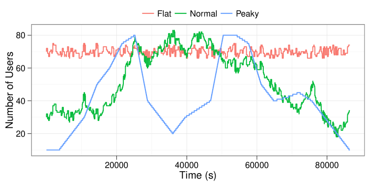
Figure 1: The three types of workloads.

• Normal day: consists of small peaks of utilisation during the start, middle, and end of work hours reflecting the time when users check their e-mails and websites, for example. Outside these intervals, but still in work hours, this workload remains around the peak values, while outside the working hours it goes down significantly.

• Flat day: consists of a flat number of users during the whole period. Although unrealistic in most real-world environments, this load is used to evaluate a scenario with near constant load.

• Peaky day: consists of tipping workload peaks, a configuration that is realistic and reflects the situation where impacting news reach the outside world, causing users to access a service more often. The configuration is used to test the solution’s behaviour handling stress situations.

For each workload we vary the number of resources used by the Cloud service, thus allowing for evaluating the system under different stress levels. When using the system, a user makes a request and waits for its results before making a new request, with a think time between receiving results and making another request uniformly distributed between 0 and 100 seconds. To facilitate the analysis and comparison among the techniques, the length of jobs is constant (10 seconds).

Previous interactions with the service are used to build a user’s expectation on how the service should respond, and how quickly a request should be processed. The model that defines a user’s expectation on the response time of a request uses two moving averages, (i) an Exponential Weighted Moving Average (EWMA) of the previous 20 response times, with $\alpha=0.8$; and (ii) an average of the past 4 response times, used to eliminate outliers. When a request completes, if the response time is 30% below the average of the past 4 response times, then the EWMA is not updated, though the value is considered in future iterations. In essence, this model states that the user expects the service to behave similar to previous interactions, with a higher weigh to more recent requests. Even though changes in response time affect the user’s perception of the service, she disregards large deviations in service quality; unless they become common. As we believe that in real conditions, users would not correctly average their past response times (i.e. they may not recall past experiences well) we add tolerance of 20% to the estimate of response time provided by the model.

We consider that users have different levels of patience — If you ever listened to customers’ complaints in a supermarket queue in a busy city like Sao Paulo you probably know what we are referring to. Hence, a user’s response time threshold—i.e. the maximum response time that she considers acceptable—is randomly selected between 40 seconds and 60 seconds. The provider stores information on how it served previous requests made by a user and users the same model described above to compute an estimate of what it believes the user’s expectation to be. 60 seconds is also what the provider considers to be the maximum acceptable response time that satisfies the service users. However, for EAS and PAS, if a request’s response is above 60 seconds, the EWMA is updated with 40 seconds, which may give the user priority the next time she submits a request. It is a way the scheduler finds to penalise itself for yielding a response time too far from what it believes the user’s expectation to be.

3.2 Result Analysis

Figure 2 depicts the Patience Indexes (as defined in Section 2.2) of requests when below 1.0 for flat, normal, and peaky workloads. The lower the values the more unhappy the users. We observe that for high and low system load (i.e. r4–6 and r16–20), all strategies perform similarly, whereas for the other loads PAS and EAS produce higher Patience Indexes than FIFO. Under high loads, most requests are completed after the expected response time, thus not allowing the scheduler to exchange the order of the requests in the waiting queue in subsequent task submissions. On the other hand, a very light system contains a short (or empty) waiting queue; hence not having requests to be sorted.

The impact of the scheduling strategies becomes evident when the system is almost fully loaded, i.e. when the waiting queue is not empty and there are requests that can quickly be assigned to resources. In this scenario, requests with longer response time expectations can give room to tasks from impatient users. The FIFO strategy does not explore the possibility of modifying the order of requests considering user patience.

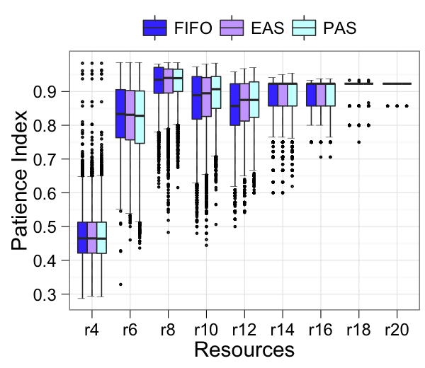
(a) Flat.

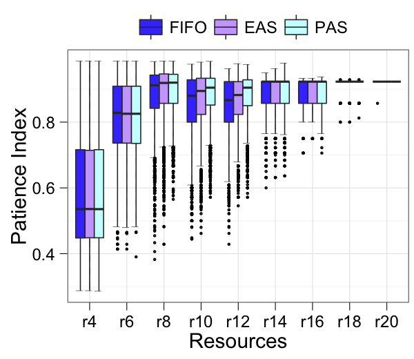
(b) Normal.

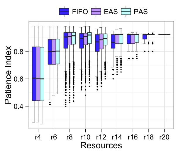
(c) Peaky.

Figure 2: Patience index under different workloads.

Figure 3 presents the percentage of requests that were served considerably later than the expected response time, that is, when their Patience Index tends to zero. Such requests represent the stage where users’ level of happiness is decreasing considerably. The percentage was normalised by the total number of requests for each resource setting for all strategies. The behaviour of this metric follows the patience indexes, but it highlights the impact of the proposed strategies have on users with very low patience levels.

(a) Flat.

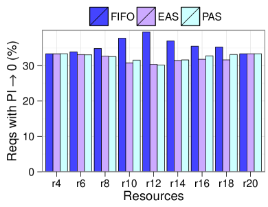
(b) Normal.

(c) Peaky.

Figure 3: % of requests whose patience index tends to 0.

4 Related Work

Scheduling is a well-studied topic in several domains, including resource management for clusters, grids, and more recently Cloud computing. Commonly used algorithms include First-In First-Out, priority-based, deadline-driven, some hybrids using backfilling techniques [17], among others [5, 9]. In addition to priority and deadline, other factors have been considered, such as fairness [8], energy-consumption [15], and context-awareness [2]. Moreover, utility functions were used to model how the importance of results to users varies over time [13, 4] and attention scarcity was leveraged to determine priority of service requests in the Cloud [14].

User behaviour has been explored for optimising resource management in the context of Web caching and page pre-fetching[10, 1, 3, 7]. The goal is to understand how users access web pages, investigate their tolerance level on delays, and pre-fetch or modify page content to enhance user experience. Techniques in this area focus mostly on web content and minimising response time of user requests.

Service research has also investigated the impact of delays on users’ behaviour. For instance, Taylor [16] described the concept of delays and surveyed passengers affected by delayed flights to test their hypotheses. Brown et al. [6] and Gans et al. [11] investigated the impact of service delays in call centres. In behavioural economics, Kahneman and Tversky [12] introduced prospect theory to model how people make choices in situations that involve risk or uncertainty.

5 Conclusions

We presented Patience-Aware Scheduling (PAS) and Expectation-Aware Scheduling (EAS) strategies that use estimates on users’ level of tolerance or patience to define the order in which resources are assigned to requests.

We compared the EAS with FIFO analytically and showed that it is not trivial to choose between both algorithms. In fact, the quality of the scheduling plans they produce depends strongly on users’ level of happiness with a service and tolerance to delays. Deeper analytical results will probably require a better understanding and more precise characterisation of these two aspects. Our computational evaluation shows that both PAS and EAS perform better than FIFO under peak load scenarios, and that PAS is slightly better than EAS.

Several aspects can be explored in future work. The PAS strategy works basically as a greedy algorithm, and in spite of the challenges involving the prediction of resolution times for tasks that are still in the queue, we believe that the use of more advanced data structures and/or algorithms may improve the quality of its scheduling plans.

References

- [1] Alt, F., Sahami Shirazi, A., Schmidt, A., Atterer, R.: Bridging waiting times on web pages. In: 14th Int. Conf. on Human-computer interaction with mobile devices and services (MobileHCI’12). pp. 305–308. ACM, New York, NY, USA (2012)
- [2] Assunção, M.D., Netto, M.A.S., Koch, F., Bianchi, S.: Context-aware job scheduling for cloud computing environments. In: 5th IEEE Int. Conf. on Utility and Cloud Computing (UCC) (2012)
- [3] Atterer, R., Wnuk, M., Schmidt, A.: Knowing the user’s every move: user activity tracking for website usability evaluation and implicit interaction. In: 15th Int. Conf. on World Wide Web (WWW’06). pp. 203–212. ACM, New York, NY, USA (2006)
- [4] AuYoung, A., Rit, L., Wiener, S., Wilkes, J.: Service contracts and aggregate utility functions. In: 15th IEEE Int. Symp. on High Performance Distributed Computing (HPDC’06) (2006)
- [5] Braun, T.D., Siegel, H.J., Beck, N., Bölöni, L.L., Maheswaran, M., Reuther, A.I., Robertson, J.P., Theys, M.D., Yao, B., Hensgen, D., et al.: A comparison of eleven static heuristics for mapping a class of independent tasks onto heterogeneous distributed computing systems. Journal of Parallel and Distributed computing 61(6), 810–837 (2001)
- [6] Brown, L., Gans, N., Mandelbaum, A., Sakov, A., Shen, H., Zeltyn, S., Zhao, L.: Statistical analysis of a telephone call center: A queueing-science perspective. Journal of the American Statistical Association 100, 36–50 (2005)
- [7] Cunha, C.R., Jaccoud, C.F.B.: Determining www user’s next access and its application to pre-fetching. In: 2nd IEEE Symp. on Computers and Communications (ISCC ’97). pp. 6–. Washington, DC, USA (1997)
- [8] Doulamis, N.D., Doulamis, A.D., Varvarigos, E.A., Varvarigou, T.A.: Fair scheduling algorithms in grids. IEEE Transactions on Parallel and Distributed Systems 18(11), 1630–1648 (2007)
- [9] Feitelson, D.G., Rudolph, L., Schwiegelshohn, U., Sevcik, K.C., Wong, P.: Theory and practice in parallel job scheduling. In: Workshop on Job Scheduling Strategies for Parallel Processing (JSSPP’97). pp. 1–34. Springer (1997)
- [10] Galletta, D.F., Henry, R.M., McCoy, S., Polak, P.: Web site delays: How tolerant are users? Journal of the Association for Information Systems 5(1), 1–28 (2004)
- [11] Gans, N., Koole, G., Mandelbaum, A.: Telephone call centers: Tutorial, review, and research prospects. Manufacturing & Service Operations Management 5(2), 79–141 (2003)
- [12] Kahneman, D., Tversky, A.: Prospect theory: An analysis of decision under risk. Econometrica: Journal of the Econometric Society pp. 263–291 (1979)
- [13] Precise and Realistic Utility Functions for User-Centric Performance Analysis of Cchedulers (2007)
- [14] Netto, M.A.S., Assunção, M.D., Bianchi, S.: Leveraging attention scarcity to improve the overall user experience of cloud services. In: Proceedings of the IFIP 9th International Conference on Network and Service Management (CNSM’13) (2013)
- [15] Pineau, J.F., Robert, Y., Vivien, F.: Energy-aware scheduling of bag-of-tasks applications on master–worker platforms. Concurrency and Computation: Practice and Experience 23(2), 145–157 (2011)
- [16] Taylor, S.: Waiting for service: the relationship between delays and evaluations of service. The Journal of Marketing pp. 56–69 (1994)
- [17] Tsafrir, D., Etsion, Y., Feitelson, D.G.: Backfilling using system-generated predictions rather than user runtime estimates. IEEE Transactions on Parallel and Distributed Systems 18(6), 789–803 (2007)