Null tests of the cosmological constant using supernovae

Abstract

The standard concordance model of the Universe is based on the cosmological constant as the driver of accelerating expansion. This concordance model is being subjected to a growing range of inter-locking observations. In addition to using generic observational tests, one can also design tests that target the specific properties of the cosmological constant. These null tests do not rely on parametrizations of observables, but focus on quantities that are constant only if dark energy is a cosmological constant. We use supernova data in null tests that are based on the luminosity distance. In order to extract derivatives of the distance in a model-independent way, we use Gaussian Processes. We find that the concordance model is compatible with the Union 2.1 data, but the error bars are fairly large. Simulated datasets are generated for the DES supernova survey and we show that this survey will allow for a sharper null test of the cosmological constant if we assume the Universe is flat. Allowing for spatial curvature degrades the power of the null test.

I Introduction

The simplest model that can explain the apparent acceleration of the Universe is the ‘concordance’ $\Lambda$CDM model, with $\Omega_{{m}}\approx 0.3$ and zero spatial curvature $\Omega_{{K}}=0$. The concordance model is consistent with all observations to date Ade:2013zuv . Current observations favour a dark energy model with equation of state $w(z)\approx-1$, although there are modified gravity models with no dark energy that are also consistent with the data Clifton:2011jh . Next-generation experiments such as DES Abbott:2005bi , LSST Abell:2009aa , EUCLID Laureijs:2011gra and the SKA Blake:2004pb , are expected to dramatically improve on current constraints and introduce new observables.

It is typical to parametrize $w(z)$ in order to differentiate between various dark energy models, or to parametrize background and perturbation variables to test classes of modified gravity models. A complementary approach is to test the consistency of the concordance model itself, independent of the values of $\Omega_{{m}}$ and $\Omega_{{K}}$. A range of null tests designed specifically to probe various aspects of the concordance model have been introduced (see e.g. Clarkson:2007pz ; Uzan:2008qp ; Sahni:2008xx ; Zunckel:2008ti ; Shafieloo:2009hi ; Clarkson:2009jq ; Nesseris:2010ep ; Seikel:2012cs and Clarkson:2012bg for a review).

Type Ia Supernovae (SNIa) are the best distance indicators to probe the expansion history of the Universe. These ‘standardizable candles’ can be observed to high redshift, and have produced convincing evidence that the Universe has undergone a recent phase of accelerated expansion. Current samples of SNIa (e.g. Conley:2011ku ; Suzuki:2011hu ; Campbell:2012hi ; Scolnic:2013aya ; Rest:2013bya ) comprise several hundred SNIa with $z<1.8$. Forthcoming surveys of SNIa, such as DES Bernstein:2011zf , will produce well-measured light-curves for over 4000 SNIa, improving the cosmological constraints by an order of magnitude.

In this paper we use luminosity distances $d_{L}(z)$ determined from SNIa observations to test the consistency of the concordance model, through a set of null tests. Reconstructing the expansion history of the Universe in a model-independent fashion is essential for these tests. To do this, we use Gaussian Processes (GP), which have previously been used to reconstruct $w(z)$ from SNIa luminosity distances Holsclaw:2010nb ; Holsclaw:2010sk ; Holsclaw:2011wi ; Seikel:2012uu ; Shafieloo:2012ht . Our analysis is built on Seikel:2012cs , which used $H(z)$ data from the baryon acoustic oscillation (BAO) scale and galaxy ages to test the validity of the concordance model. We use GaPP (Gaussian Processes in Python), a package developed by Seikel and introduced in Seikel:2012uu .

The tests based on $H(z)$ are potentially stronger discriminators of the concordance model than those using SNIa data, since the null tests using $d_{L}(z)$ require higher derivative terms than those using $H(z)$. However, null tests based on direct distance measurements currently have the advantage that the data sets are much larger and the errors are smaller.

II Null tests of $\Lambda$CDM – theory

The Friedmann equation,

$$\frac{H^{2}(z)}{H^{2}_{0}}=\Omega_{{m}}(1+z)^{3}+\Omega_{{K}}(1+z)^{2}$$

$$~{}~{}+(1-\Omega_{{m}}-\Omega_{{K}})\exp\left[3\int_{0}^{z}\frac{1+w(z{{}^{\prime}})}{1+z{{}^{\prime}}}dz{{}^{\prime}}\right]\!,$$ (1)

determines the Hubble rate $H$ in terms of today’s values for the density parameters for matter $\Omega_{{m}}$ and curvature $\Omega_{{K}}$. This is integrated over to obtain the luminosity distances of SNIa:

$$d_{L}(z)=\frac{(1+z)}{H_{0}\sqrt{-\Omega_{{K}}}}\sin\left(\sqrt{-\Omega_{{K}}}\int_{0}^{z}\frac{dz^{\prime}}{H(z^{\prime})/H_{0}}\right).$$ (2)

The equation of state parameter of dark energy, $w=p_{\rm de}/\rho_{\rm de}$, can be expressed in terms of the dimensionless comoving luminosity distance,

$$D(z)\equiv H_{0}(1+z)^{-1}d_{L}(z),$$ (3)

as Starobinsky:1998fr ; Nakamura:1998mt ; Huterer:1998qv :

$$\!\!\!\!w(z)=\Big{\{}2(1+z)(1+\Omega_{{K}}D^{2})D^{\prime\prime}-[(1+z)^{2}\Omega_{{K}}D^{\prime 2}$$

$${}\!\!\!\!+2(1+z)\Omega_{{K}}DD^{\prime}-3(1+\Omega_{{K}}D^{2})]D^{\prime}\Big{\}}/$$ (4)

$${}\!\!\!\!\Big{\{}3\{(1+z)^{2}[\Omega_{{K}}+(1+z)\Omega_{{m}}]D^{\prime 2}-(1+\Omega_{{K}}D^{2})\}D^{\prime}\Big{\}}.$$

Given an observed distance-redshift relationship $D(z)$, it is possible to reconstruct the equation of state of dark energy and test the $\Lambda$CDM model Seikel:2012uu . However, a disadvantage of this method is that it depends on the values of the density parameters, $\Omega_{{m}}$ and $\Omega_{{K}}$, which must be measured independently Seikel:2012uu .

To avoid this problem and test $\Lambda$CDM using SNIa data, we use the consistency tests introduced in Zunckel:2008ti (see also Sahni:2008xx ; Shafieloo:2009hi ). Following this approach, we test the null hypothesis that the expansion of the universe can be described by a flat or a curved $\Lambda$CDM model.

The assumptions underlying the consistency tests and the null hypothesis are: (1) the universe is homogeneous and isotropic on large scales; (2) gravity obeys general relativity; (3) the universe contains cold matter (with $w=0$) and dark energy. Photons and neutrinos can be included ($\Omega_{\gamma}$, $\Omega_{\nu}$ are known independently, from CMB data), but it is reasonable to neglect radiation at the low redshifts probed by SNIa data. Detection of a deviation from the consistency tests would imply a violation of at least one of these assumptions: (1) large-scale nonlinear inhomogeneity or anisotropy; (2) modified gravity; (3) dynamical dark energy ($w\neq-1$), or alternatively, a cosmological constant plus an unknown additional species with equation of state which deviates from that of cold matter, curvature or vacuum energy. Any of these possibilities imply that the standard $\Lambda$CDM is ruled out. Note that the tests cannot identify which of these possibilities applies.

For a flat concordance model, i.e. $w=-1$ and $\Omega_{{K}}=0$, from (2) we find that

$$\Omega_{{m}}\left[(1+z)^{3}-1\right]D^{\prime 2}=1-D^{\prime 2}.$$ (5)

If we define

$$\mathcal{O}_{m}^{(1)}(z) ~{}=\frac{1-D^{\prime}(z)^{2}}{[(1+z)^{3}-1]D^{\prime}(z)^{2}},$$ (6)

then

$$\mathrm{flat~{}\Lambda CDM~{}implies~{}}\mathcal{O}_{m}^{(1)}(z)=\Omega_{{m}}.$$ (7)

Thus we obtain a null test of the concordance model:

$$\mathcal{O}_{m}^{(1)}(z)\neq\Omega_{{m}}~{}\mathrm{falsifies~{}flat~{}\Lambda CDM}.$$ (8)

Any variation of $\mathcal{O}_{m}^{(1)}(z)$ with redshift reflects an inconsistency between the flat $\Lambda$CDM model and observations. To detect evolution of $\mathcal{O}_{m}^{(1)}$ with redshift we can differentiate $\mathcal{O}_{m}^{(1)}(z)$, from which we define the additional diagnostic:

$$\mathcal{L}^{(1)}(z) ~{}=(1+z)^{-6}\Big{\{}2\left[(1+z)^{3}-1\right]D^{\prime\prime}(z)$$

$$~{}~{}+3(1+z)^{2}D^{\prime}(z)\left[1-D^{\prime}(z)^{2}\right]\Big{\}},$$ (9)

which vanishes if and only if $d\mathcal{O}_{m}^{(1)}/dz=0$. The factor $(1+z)^{-6}$ (which was not used in Zunckel:2008ti ), ensures stability of the errors (see below). If $\mathcal{L}^{(1)}$ is nonzero at any redshift, then observations are incompatible with $\Lambda$CDM:

$$\mathcal{L}^{(1)}\neq 0~{}\mathrm{falsifies~{}flat~{}\Lambda CDM}.$$ (10)

We can extend this approach to include spatial curvature, and derive null tests for general (curved) $\Lambda$CDM. Using (1), (2) and (II) with $w(z)=-1$, and solving for $\Omega_{{m}}$ and $\Omega_{{K}}$, we find Clarkson:2009jq ; Clarkson:2012bg :

$$\Omega_{{m}} ~{}=2\Upsilon(z)\Big{\{}\left[(1+z)^{2}-D^{2}-1\right]D^{\prime\prime}$$

$$~{}~{}-\left(D^{\prime 2}-1\right)\left[(1+z)D^{\prime}-D\right]\Big{\}}\equiv\mathcal{O}_{m}^{(2)}(z),$$ (11)

$$\Omega_{{K}} ~{}=\Upsilon(z)\Big{\{}2\left[1-(1+z)^{3}\right]D^{\prime\prime}$$

$$~{}~{}+3D^{\prime}\left(D^{\prime 2}-1\right)(1+z)^{2}\Big{\}}\equiv\mathcal{O}_{{K}}(z).$$ (12)

Here $\Upsilon(z)$ is defined by

$$\Upsilon^{-1} ~{}=-2\left[1-(1+z)^{3}\right]D^{2}D^{\prime\prime}$$

$$~{}-\Big{\{}(1+z)\left[(1+z)^{3}-3(1+z)+2\right]D^{\prime 2}$$

$$~{}-2\left[1-(1+z)^{3}\right]DD^{\prime}-3(1+z)^{2}D^{2}\Big{\}}D^{\prime}.$$ (13)

Then we have

$$\mathcal{O}_{m}^{(2)}(z)\neq\Omega_{{m}}~{}\mathrm{falsifies~{}curved~{}\Lambda CDM},$$ (14)

$$\mathcal{O}_{{K}}^{(2)}(z)\neq\Omega_{{K}}~{}\mathrm{falsifies~{}curved~{}\Lambda CDM}.$$ (15)

These are not independent tests: the derivative of $\mathcal{O}_{{K}}^{(2)}$ vanishes if and only if the derivative of $\mathcal{O}_{m}^{(2)}$ vanishes. Hence we need only a single diagnostic for vanishing derivative. We use the derivative of $\mathcal{O}_{m}^{(2)}$ to define

$$\mathcal{L}^{(2)} ~{}=(1+z)^{-6}D^{\prime 2}\Big{\{}D\Big{[}-3\left(1+z\right)$$

$$~{}\times\left(D^{\prime 2}-1\right)\left(2D^{\prime}+3(1+z)D^{\prime\prime}\right)$$

$$~{}+2zD^{\prime\prime\prime}\Big{(}3+z(3+z)\Big{)}\Big{]}+9(1+z)^{2}D^{2}D^{\prime\prime 2}$$

$$~{}+3(1+z)D^{2}D^{\prime}\Big{(}2D^{\prime\prime}-(1+z)D^{\prime\prime\prime}\Big{)}$$

$$~{}+6(1+z)^{2}D^{\prime 2}\left(D^{\prime 2}-1\right)-\Big{[}3z^{2}(3+z)D^{\prime\prime 2}$$

$$~{}+zD^{\prime}\Big{(}z(3+z)D^{\prime\prime\prime}-6(2+z)D^{\prime\prime}\Big{)}\Big{]}(1+z)\Big{\}},$$ (16)

which vanishes if and only if $d\mathcal{O}_{m}^{(2)}/dz=0$. (Again we use the pre-factor to stabilize the errors.) Then we have the null test for curved $\Lambda$CDM:

$$\mathcal{L}^{(2)}(z)\neq 0~{}\mathrm{falsifies~{}curved~{}\Lambda CDM}.$$ (17)

In principle, $\mathcal{L}^{(1)}$ and $\mathcal{L}^{(2)}$ provide no additional information compared to $\mathcal{O}_{m}^{(1)}$ and $\mathcal{O}_{m}^{(2)}$. However, it is easier to detect a deviation from zero than to confirm that a quantity is constant, especially since the exact value of this constant is not known a priori. The disadvantage of $\mathcal{L}^{(1)}$ and $\mathcal{L}^{(2)}$ is that they require higher derivatives than $\mathcal{O}_{m}^{(1)}$ and $\mathcal{O}_{m}^{(2)}$, which are more challenging to constrain.

Another problem with $\mathcal{L}^{(1)}$ and $\mathcal{L}^{(2)}$ is the degeneracy between $w$ and $\Omega_{m}$: a model with redshift dependent $w$ can be formally consistent with $\Lambda$CDM within the error bars of the reconstruction if the value of $\Omega_{m}$ is adjusted accordingly. Such cases can only be identified with the $\mathcal{O}_{m}$ tests, but not with $\mathcal{L}$ (see section IV for details).

Note that $\mathcal{L}^{(1)}$ and $\mathcal{L}^{(2)}$ are not identical to $d\mathcal{O}_{m}^{(1)}/dz$ and $d\mathcal{O}_{m}^{(2)}/dz$, respectively. Starting from these two derivatives, we have neglected the denominators, which add significant noise to the tests without adding extra information, and used a pre-factor $(1+z)^{-6}$ to obtain $\mathcal{L}^{(1)}$ and $\mathcal{L}^{(2)}$. We are free to do this without loss of generality, since we are testing the equality of these quantities with zero. As a consequence, the error bands of the reconstructions do not necessarily increase with redshift as one might expect, and the size of the errors of $\mathcal{L}^{(1)}$ and $\mathcal{L}^{(2)}$ are not directly comparable. In addition, the errors added from extra redshift factors are small when we have spectroscopic redshift measurements.

III Null tests using SNIa data

To apply these null tests using current datasets, it is essential to choose a model-independent method to reconstruct $D(z)$ and its derivatives. For this purpose, we use GP (via the GaPP code Seikel:2012uu ) to smooth the data and reconstruct the derivatives.

III.1 Gaussian Processes

GP provide a distribution over functions that are suitable to describe the data. At each point $z_{i}$, the distribution of function values $f(z_{i})$ is a Gaussian. Thus the reconstruction consists of a mean function with Gaussian error bands. The function values at different points are correlated by a covariance function $k(z,\tilde{z})$, which depends on a set of hyperparameters (e.g. the characteristic length scale $\ell$ and the signal variance $\sigma_{f}$). This also provides a robust way to estimate derivatives of the function in a stable manner.

In contrast to parametric methods, GP do not assume a specific form for the reconstructed function. Instead only typical changes of the function are considered. The hyperparameter $\ell$ corresponds roughly to the distance one needs to move in input space before the function value changes significantly, while $\sigma_{f}$ describes typical changes in the function value.

The choice of covariance function affects the reconstruction to some extent. A general purpose covariance function is the squared exponential covariance function $k(z,\tilde{z})=\sigma_{f}^{2}\exp\left[-(z-\tilde{z})^{2}/(2\ell^{2})\right]$. However, here we use the Matérn ($\nu=9/2$) covariance function:

$$k(z,\tilde{z}) = \sigma_{f}^{2}\exp\Big{(}-\frac{3\,|z-\tilde{z}|}{\ell}\Big{)}$$ (18)

$$~{}\times\Big{[}1+\frac{3\,|z-\tilde{z}|}{\ell}+\frac{27(z-\tilde{z})^{2}}{7\ell^{2}}$$

$$~{}~{}~{}~{}~{}~{}+\frac{18\,|z-\tilde{z}|^{3}}{7\ell^{3}}+\frac{27(z-\tilde{z})^{4}}{35\ell^{4}}\Big{]}.$$

For a given covariance function, the probability distribution of the hyperparameters depends only on the data. It is necessary either to marginalize over the hyperparameters $\sigma_{f}$ and $\ell$, or to fix the hyperparameters to their maximum likelihood values. Here we choose the latter approach, which is a good approximation and computationally much less expensive than marginalization.

We choose the Matérn ($\nu=9/2$) covariance function because it leads to the most reliable results amongst the covariance functions that we have tested. Here, “reliable” means the following: For various assumed cosmological models and many realizations of mock data sets, the assumed model on average lies within the reconstructed 1-$\sigma$ limits for approximately 68% of the redshift range (and within the reconstructed 2-$\sigma$ limits for $\sim 95$% of the redshift range). These values are theoretically expected, thus making Matérn ($\nu=9/2$) a reliable covariance function for our purposes. A detailed analysis regarding the optimal choice of covariance function can be found in Seikel:2013fda . (Note that these results only apply to GP reconstructions using $D$ measurements. When applying GP to other data, another covariance function might be more reliable.)

We follow Seikel:2012uu ; Seikel:2012cs , which contain a summary of the technical details of GP. The only difference in our approach here is that we use the Matérn covariance function (18) instead of the squared exponential. (For detailed reviews of GP, see Rasmussen ; MacKay .)

III.2 Application to real data

We now apply GP to the Union 2.1 dataset Suzuki:2011hu and determine the current constraints on the consistency of $\Lambda$CDM. This data set comprises $580$ SNIa, with $0.015<z<1.5$, and includes a covariance matrix which incorporates a systematic uncertainty.

The distance modulus, $\mu=m-M$, is the difference between the observed magnitude $m(z)$ and the absolute magnitude of an object $M$, and is given by

$$\mu(z)+5\log H_{0}-25=5\log\left[(1+z)D(z)\right].$$ (19)

We choose $H_{0}=70\,$kms^-1Mpc^-1, as in  Suzuki:2011hu . Note that $H_{0}$ and $M$ are degenerate in (19) so we can fix $H_{0}$ and only consider the uncertainties in $M$ which are included in the covariance matrix of the Union 2.1 dataset Suzuki:2011hu  – this includes the errors on $H_{0}$. We convert $\mu$ to $D$ and add the theoretical values $D(z=0)=0$ and $D^{\prime}(z=0)=1$ to the data set.

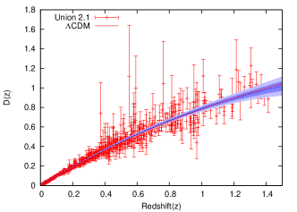
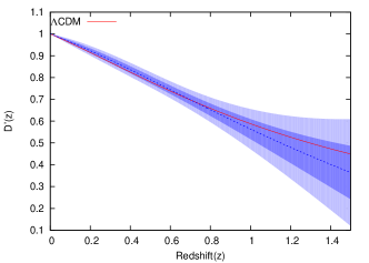
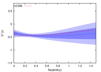
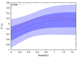
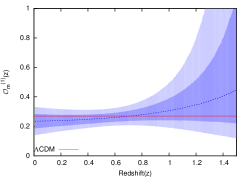
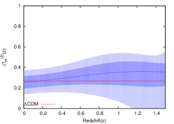
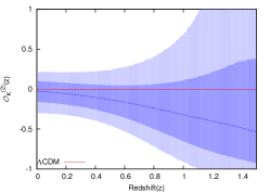
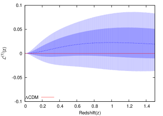
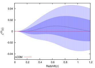
Figure 1 shows the reconstructed $D(z)$ and its first three derivatives for the Union 2.1 data set, while Figure 2 shows the inferred reconstructions for $\mathcal{O}_{m}^{(1)}$, $\mathcal{O}_{m}^{(2)}$ and $\mathcal{O}_{K}^{(2)}$. Figure 3 shows the reconstruction of $\mathcal{L}^{(1)}$ and $\mathcal{L}^{(2)}$.

The errors on the reconstructed distances in Figure 1 increase with increasing order of derivative. For example, at $z=1.5$, the standard deviation is 0.05 for the reconstruction of $D$, 0.12 for $D^{\prime}$, 0.22 for $D^{\prime\prime}$, and 0.29 for $D^{\prime\prime\prime}$. The near-constancy of the errors on $D^{\prime\prime\prime}$ reflect the fact that we are unable to constrain rapid variations (carried via higher derivatives) on scales below a typical length scale, which is roughly associated with $\ell$. By using Gaussian Processes the scale $\ell$ and the resulting smoothness of the reconstruction is driven purely by the data. Where there is insufficient evidence for rapid variations, a smooth function will result, which we see in the second and third derivatives. Further analysis of the redshift-dependence of the errors can be found in the appendix.

Figure 1: Gaussian processes reconstruction of $D$, $D^{\prime}$ (top) and $D^{\prime\prime}$, $D^{\prime\prime\prime}$ (bottom) for Union 2.1 data. The red (solid) line is flat $\Lambda$CDM with $\Omega_{{m}}=0.27$. The blue (dashed) line is the mean of the reconstruction. Shaded areas give $95\%$ (light) and $68\%$ (dark) confidence limits of the reconstructed function.

Figure 2: Reconstruction of $\mathcal{O}_{m}^{(1)}$ (left), $\mathcal{O}_{m}^{(2)}$ (middle) and $\mathcal{O}_{K}^{(2)}$ (right) for Union 2.1 data. Lines and shadings are as in Fig. 1.

Figure 3: Reconstruction of $\mathcal{L}^{(1)}$ (left) and $\mathcal{L}^{(2)}$ (right) for Union 2.1 data. Lines and shadings are as in Fig. 1.

III.3 Mock data

To demonstrate the ability of the null tests to distinguish between different cosmological models when applied to future SNIa datasets, we produce mock catalogues for two fiducial models:

• Flat $\Lambda$CDM

• Dynamical dark energy model with $\Omega_{{K}}=0$ and

  $$w(z)=\frac{1}{2}\Big{\{}-1+\tanh\Big{[}3\Big{(}z-\frac{1}{2}\Big{)}\Big{]}\Big{\}}.$$ (20)

We take $\Omega_{{m}}=0.3$. Using the redshift distribution and scatter anticipated by the Dark Energy Survey (DES) Bernstein:2011zf , we simulate $\sim 4000$ data points in the redshift range $0<z<1.2$. Note that the scatter only includes statistical errors.

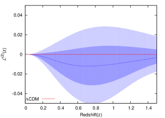
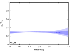
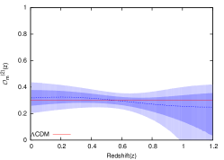
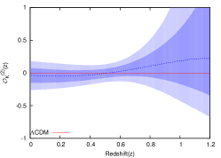
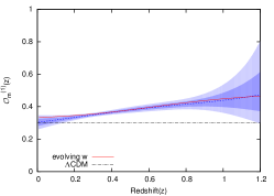
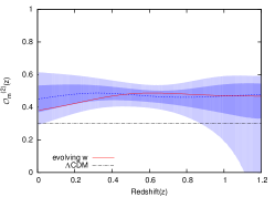
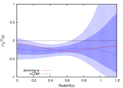
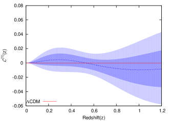
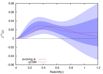
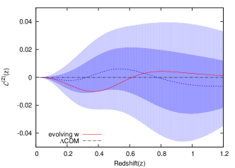
For each of the two simulated data sets, we reconstruct $D(z)$ and its derivatives and apply the null tests. Figure 4 shows the constraints and uncertainties on $\mathcal{O}_{m}^{(1)}$, $\mathcal{O}_{m}^{(2)}$ and $\mathcal{O}_{K}^{(2)}$ for both models, while Figure 5 shows the results for $\mathcal{L}^{(1)}$ and $\mathcal{L}^{(2)}$.

Figure 4: $\mathcal{O}_{m}^{(1)}$ (left), $\mathcal{O}_{m}^{(2)}$ (middle) and $\mathcal{O}_{K}^{(2)}$ (right) reconstructed using simulated DES data, and assuming $\Lambda$CDM (top) and the evolving $w$ in (20) (bottom).

Figure 5: Reconstruction of $\mathcal{L}^{(1)}$ (left) and $\mathcal{L}^{(2)}$ (right) for simulated DES data, and assuming $\Lambda$CDM (top) and the evolving $w$ in (20) (bottom). Due to the degeneracy between $w$ and $\Omega_{m}$, the reconstruction of $\mathcal{L}^{(2)}$ for the model with evolving dark energy is consistent with $\Lambda$CDM. However, the inferred values of $\Omega_{m}$ and $\Omega_{K}$ differ significantly from the input value as can be seen in Fig. 4.

IV Discussion

We have introduced an approach to applying null tests of the $\Lambda$CDM models (flat and curved). Using a GP technique to reconstruct the distance-redshift relationship and its derivatives from SNIa data sets in a model-independent fashion, we have shown that the flat concordance model is consistent with current data, falling within the 1$\sigma$ limits. The null tests are stronger if we assume flatness, as expected.

For the Union 2.1 dataset, the consistency tests are in good agreement with a constant, indicating no evidence of a deviation from a flat $\Lambda$CDM model (see Figures 2 and 3). For the $\mathcal{O}_{m}^{(1)}$ and $\mathcal{O}_{m}^{(2)}$ tests we find a value for $\Omega_{{m}}\sim 0.27$. $\mathcal{O}_{K}^{(2)}$ is consistent with zero, as expected for flat $\Lambda$CDM. Due to the limited number of SNIa in the Union 2.1 sample and the model-independent method we use, the reconstructed uncertainties are significant.

For a mock data set based on the DES supernova survey, we find that our approach can distinguish between competing cosmological models. Using a simulated sample drawn from a flat $\Lambda$CDM model, the recovered distribution of $\mathcal{O}_{m}^{(1)}$ is constant over the redshift range considered (Figure 4), consistent with $\mathcal{O}_{m}^{(1)}=\Omega_{{m}}$. For the evolving $w$ model of (20), $\mathcal{O}_{m}^{(1)}$ deviates strongly from a constant value, so that flat $\Lambda$CDM would be disfavoured. This is confirmed by the deviation of $\mathcal{L}^{(1)}$ from zero in Figure 5.

When spatial curvature is allowed, the constraints from the null tests tend to be weakened, as would be expected by the degeneracy introduced by the extra degree of freedom Clarkson:2007bc . For a flat $\Lambda$CDM fiducial model, the reconstructed distribution of $\mathcal{O}_{m}^{(2)}$ and $\mathcal{O}_{K}^{(2)}$ are consistent with being constant and equal to $\Omega_{{m}}$ and $\Omega_{K}$ (Figure 4), respectively, confirming that the model does not deviate from $\Lambda$CDM, as anticipated. But the errors are significantly larger when curvature is allowed.

For the evolving $w$ fiducial model, the reconstructions of $\mathcal{O}_{m}^{(2)}$ and $\mathcal{O}_{K}^{(2)}$ are consistent with constants (Figure 4) – but these constant values differ significantly from the input values of $\Omega_{{m}}$ and $\Omega_{K}$, respectively. The evolving $w$ model can erroneously be interpreted as a $\Lambda$CDM model with a large matter density $\Omega_{{m}}$ and negative curvature $\Omega_{{K}}$. Consequently, the reconstruction of $\mathcal{L}^{(2)}$ (Figure 5) is consistent with a constant, indicating that $\Lambda$CDM is not disfavoured. In both cases, the errors are large and the null tests are degraded.

This problem reflects the degeneracy between the density parameters and the dark energy equation of state (see also Clarkson:2007bc ; Hlozek:2008mt ; Seikel:2012uu ). The reconstructions are formally consistent with a constant, and thus with $\Lambda$CDM, due to their incorrectly inferred values. Additional constraints on the value of $\Omega_{{m}}$ and $\Omega_{{K}}$ from, for instance, BAO or CMB measurements, are needed to break this degeneracy.

V Conclusions

In this paper, we described a series of null tests that can be applied to SNIa data to determine the consistency of observations with a (flat) $\Lambda$CDM model – without the need to parametrize the equation of state of dark energy. The tests require that the distance $D$ and the diagnostics $\mathcal{O}_{m}^{(1)}$, $\mathcal{O}_{m}^{(2)}$, $\mathcal{O}_{K}^{(2)}$, $\mathcal{L}^{(1)}$ and $\mathcal{L}^{(2)}$ are reconstructed in a model-independent way. We used GP to perform these reconstructions.

We applied the null tests to the Union 2.1 SNIa data set. The results were consistent with a flat $\Lambda$CDM model (Figures 2 and 3).

Using the anticipated redshift distribution for the DES supernova survey, we produced mock data sets of 4000 SNIa, with two competing fiducial cosmological models: flat $\Lambda$CDM and an evolving $w$ model. The reconstructed distributions of $\mathcal{O}_{m}^{(1)}$ for these datasets show that the consistency tests are able to distinguish between different cosmological models, and can correctly identify deviations from $\Lambda$CDM, in the case when spatial flatness is assumed. However, allowing for spatial curvature degrades the null tests in general (although not always – see Fig. 2). The inherent degeneracy between the equation of state of dark energy and the density parameters ($\Omega_{{m}},\Omega_{{K}}$) reduces our ability to distinguish between various models. The distributions of $\mathcal{O}_{m}^{(2)}$, $\mathcal{O}_{K}^{(2)}$ and $\mathcal{L}^{(2)}$ were consistent with a constant for the evolving $w$ model (Figure 5), but the inferred values of $\Omega_{{m}}$ and $\Omega_{K}$ from the $\mathcal{O}_{m}^{(2)}$ and $\mathcal{O}_{K}^{(2)}$ distributions were unrealistic (Figure 4). The degeneracy needs to be broken using other data.

For future data sets which will have the power to probe $\Lambda$CDM at high precision, the null tests we have introduced will require further refinement. In particular, we need to develop a method of quantifying the significance of any possible deviation. This is left for future work.

*

Appendix A Redshift-dependence of the errors on the GP reconstructions

The error of the GP reconstruction of the $n$th derivative on $D$ at point $z^{*}$ is given by:

$$\!\!\!\sigma\left(D^{(n)}(z^{*})\right)=\left(k^{(n,n)}(z^{*},z^{*})\right.$$ (21)

$${}-\left.K^{(n,0)}(z^{*},\bm{Z})\left[K(\bm{Z},\bm{Z})+C\right]^{-1}K^{(0,n)}(\bm{Z},z^{*})\right)^{\frac{1}{2}}$$

Here, $\bm{Z}$ is a vector containing the locations $z_{i}$ of the data and $C$ is the covariance matrix of the data. $k$ denotes the covariance function (here, Matérn ($\nu=9/2$) as given by eq. (18)) and $K$ a matrix containing covariances between the redshift points: $[K(\bm{Z},\bm{Z})]_{ij}=k(z_{i},z_{j})$. Taking the $n$th derivative of $k$ with respect to the first argument and the $m$th derivative with respect to the second argument is denoted as $k^{(n,m)}$.

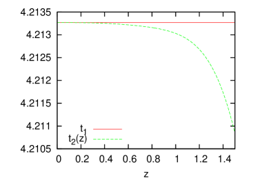
Note that the first term in the equations for the errors is constant for a given covariance function and hyperparameters. Stationary covariance functions $k(z_{i},z_{j})$, such as Matérn ($\nu=9/2$), only depend on $|z_{i}-z_{j}|$, but not on $z_{i}$ and $z_{j}$ individually. Therefore, $k^{(n,n)}(z^{*},z^{*})$ does not depend on the value of $z^{*}$.

We rewrite the equation for the errors (21) as

$$\sigma\left(D^{(n)}(z^{*})\right)=\sqrt{t_{1,n}-t_{2,n}(z^{*})}$$ (22)

where

$$t_{1,n} = k^{(n,n)}(z^{*},z^{*})$$

$$t_{2,n}(z^{*}) = K^{(n,0)}(z^{*},\bm{Z})\left[K(\bm{Z},\bm{Z})+C\right]^{-1}K^{(0,n)}(\bm{Z},z^{*})\,.$$

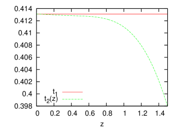
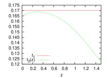
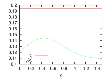
$t_{1,n}$ is determined by the covariance function and the hyperparameters. It is constant in redshift and does not explicitly depend on the data. (Note that the data are used to optimize the hyperparameters and thus indirectly affect the value of $t_{1,n}$.) $t_{2,n}(z^{*})$ is redshift dependent and also depends on the position and covariance matrix of the data.

Fig. 6 shows $t_{1}$ and $t_{2}(z^{*})$ for the reconstructions of $D$ and its derivatives. For $D$, $D^{\prime}$ and $D^{\prime\prime}$, we observe strong relative changes in $t_{1}-t_{2}(z^{*})$ with redshift. We denote the maximum value of this term within the considered redshift range as $\{t_{1}-t_{2}(z^{*})\}_{\text{max}}$ and the mean value as $\{t_{1}-t_{2}(z^{*})\}_{\text{mean}}$. Then we can quantify the redshift dependence of $t_{1}-t_{2}(z^{*})$ by the relative variation $v_{r}=\{t_{1}-t_{2}(z^{*})\}_{\text{max}}/\{t_{1}-t_{2}(z^{*})\}_{\text{mean}}$. $v_{r}=1$ implies that the errors of the reconstruction are constant, while a large value would indicate strong redshift-dependence.

We find the following results for $v_{r}$:

$$v_{r}(D) = 6.9$$

$$v_{r}(D^{\prime}) = 5.6$$

$$v_{r}(D^{\prime\prime}) = 3.2$$

$$v_{r}(D^{\prime\prime\prime}) = 1.3$$

The values for $D$, $D^{\prime}$ and $D^{\prime\prime}$ are much larger than 1, implying a strong redshift-dependence of the errors. However, for the reconstruction of $D^{\prime\prime\prime}$ the relative variation is much smaller, namely $v_{r}=1.3$. The smallness of this value can be understood by the following consideration: $t_{1}\gg t_{2}(z^{*})\,\forall z^{*}$ ensures that the absolute variations of $t_{1}-t_{2}(z^{*})$ (which are large compared to those for the lower derivatives of $D$) translate into small relative variations. Therefore, the dominance of the constant term $t_{1}$ is the main reason for the small value of $v_{r}$ and thus the near-constancy of the errors on $D^{\prime\prime\prime}$.

(a) $D(z)$

(b) $D^{\prime}(z)$

(c) $D^{\prime\prime}(z)$

(d) $D^{\prime\prime\prime}(z)$

Figure 6: Terms contributing to the calculation of the errors for the GP reconstructions of $D(z)$, $D^{\prime}(z)$, $D^{\prime\prime}(z)$ and $D^{\prime\prime\prime}(z)$. $t_{1}$ and $t_{2}(z)$ are the constant and data dependent terms, respectively, as given by eq. (22).