A-Optimal design of experiments for infinite-dimensional Bayesian linear inverse problems with regularized 0subscript0\ell_{0}-sparsificationthanks: This work was partially supported by NSF grant ARC-0941678; DOE grants DE-FC02-13ER26128, DE-SC0010518 DE-FC02-11ER26052, DE-11018096, and DE-FG02-09ER25914; and AFOSR grant FA9550-12-1-0484.

Alen Alexanderian222Institute for Computational Engineering & Sciences, The University of Texas at Austin, Austin, TX, USA    Noemi Petra22footnotemark: 2    Georg Stadler22footnotemark: 2    Omar Ghattas22footnotemark: 2 333Department of Mechanical Engineering, The University of Texas at Austin, Austin, TX, USA 444Department of Geological Sciences, The University of Texas at Austin, Austin, TX, USA
Abstract

We present an efficient method for computing A-optimal experimental designs for infinite-dimensional Bayesian linear inverse problems governed by partial differential equations (PDEs). Specifically, we address the problem of optimizing the location of sensors (at which observational data are collected) to minimize the uncertainty in the parameters estimated by solving the inverse problem, where the uncertainty is expressed by the trace of the posterior covariance. Computing optimal experimental designs (OEDs) is particularly challenging for inverse problems governed by computationally expensive PDE models with infinite-dimensional (or, after discretization, high-dimensional) parameters. To alleviate the computational cost, we exploit the problem structure and build a low-rank approximation of the parameter-to-observable map, preconditioned with the square root of the prior covariance operator. The availability of this low-rank surrogate, relieves our method from expensive PDE solves when evaluating the optimal experimental design objective function, i.e., the trace of the posterior covariance, and its derivatives. Moreover, we employ a randomized trace estimator for efficient evaluation of the OED objective function. We control the sparsity of the sensor configuration by employing a sequence of penalty functions that successively approximate the 0subscript0\ell_{0}-“norm”; this results in binary designs that characterize optimal sensor locations. We present numerical results for inference of the initial condition from spatio-temporal observations in a time-dependent advection-diffusion problem in two and three space dimensions. We find that an optimal design can be computed at a cost, measured in number of forward PDE solves, that is independent of the parameter and sensor dimensions. Moreover, the numerical optimization problem for finding the optimal design can be solved in a number of interior-point quasi-Newton iterations that is insensitive to the parameter and sensor dimensions. We demonstrate numerically that 0subscript0\ell_{0}-sparsified experimental designs obtained via a continuation method outperform 1subscript1\ell_{1}-sparsified designs.

keywords:
Optimal experimental design, A-optimal design, Bayesian inference, sensor placement, ill-posed inverse problems, low-rank approximation, randomized trace estimator, randomized SVD.
AMS:
62K05, 35Q62, 62F15, 35R30, 35Q93, 65C60.

1 Introduction

Recent advances in theory [32] and numerical algorithms (e.g., [8]) are enabling efficient solution of infinite-dimensional Bayesian inverse problems. This opens the door to consideration of the upstream question: how do we place sensors to optimally infer model parameters for large-scale problems? Here we present an efficient method for such optimal experimental design (OED) problems. Specifically, we consider Bayesian linear inverse problems governed by PDEs whose solution is the posterior probability law for a parameter field. The numerical solution of such inverse problems is challenging due to the infinite (or, when discretized, large) dimension of the parameters, ill-posedness of the inverse problem, and expensive-to-compute PDE models. The Bayesian inverse problem is by itself very challenging, but it is merely a subproblem within the OED problem, and must be solved repeatedly when using conventional OED methods. Hence, it is essential to make maximum use of the problem structure to realize efficient algorithms that are scalable, i.e., their performance—measured in number of governing (forward) PDE solves—is independent of the discretized parameter and sensor dimensions, and the discretization of the governing PDE.

When formulating an OED problem, a basic question is the precise meaning of what constitutes the design. The present work concerns computation of optimal sensor locations where observational data will be collected. A subsequent question concerns the definition of an optimal design, which leads to the choice of the design criterion. For Bayesian inverse problems, a natural choice is to seek a design that minimizes the average posterior variance of the inversion parameters, leading to the Bayesian A-optimal design criterion.

Standard references for optimal experimental design include [33, 2, 30, 28, 6]. While most of the classical texts concern problems with small or moderate parameter dimension and focus mainly on well-posed inverse problems, there has been recent interest in optimal design for large-scale ill-posed linear [16, 18] and nonlinear [20, 17] inverse problems. The numerical methods in the present paper are closest to those in [16, 18], where the authors consider finite-dimensional linear inverse problems, and develop a framework to control the mean square error of the regularized Tikhonov estimates. This leads to a design criterion that seeks to minimize the sum of the estimation bias and the variability of the estimator around its mean, which can be related to A-optimal designs. These contributions use 1subscript1\ell_{1}-penalties to control the sparsity of the design and, in [18], a low-rank singular value decomposition (SVD) of the parameter-to-observable map is used; the present paper builds on and extends both of these ideas. Further recent work that employs a Bayesian formulation includes [21, 22], where the authors use a decision theoretic design criterion, generalized polynomial chaos surrogates, and stochastic optimization to tackle nonlinear inverse problems, albeit in low to moderate parameter dimension.

In this paper, we devise scalable numerical methods for computing A-optimal designs for infinite-dimensional Bayesian linear inverse problems governed by (time-dependent) PDEs. As suggested in [18], having a low-rank SVD surrogate of the parameter-to-observable map relieves the OED method of repeated PDE solves. In the Bayesian context, we can improve on this idea and further exploit problem structure; namely, we construct a low-rank SVD representation of the parameter-to-observable map preconditioned by the square root of the prior covariance operator [8, 14]. This preconditioning amounts to filtering through the prior the information gained from the data about the model parameters. In the case of smoothing priors usually used in infinite-dimensional problems, this preconditioning results in faster spectral decay and thus allows for a more efficient low-rank approximation. The remaining steps in the solution of the OED problem use this low-rank surrogate and thus do not require additional PDE solves. As a result of a consistent discretization of the problem, i.e., one that respects the infinite-dimensional Hilbert-space structure, the numerical rank of the prior-preconditioned parameter-to-observable map is bounded with respect to the discretized parameter dimension.

We consider a finite number of candidate locations for the placement of sensors; the optimal configuration is a sparse subset of these locations. To each candidate sensor location we assign a non-negative number that weights the observation from that sensor. Finding an optimal design then amounts to choosing an optimal weight vector; a weight of 0 indicates absence of a sensor and a weight of 1 corresponds to a sensor being placed at that location. For computational convenience, we allow the weights to take on any value in [0,1]01[0,1], and use a sparsifying penalty to control the number of nonzero weights, and thus, the number of allocated sensors. One option for such a penalty is the 1subscript1\ell_{1}-norm; see, e.g., [16, 20, 18]. This approach, however, does not lead to a binary (i.e., 0–1) design. Motivated by continuation methods used in topology optimization [4, 5], we propose to solve a sequence of OED problems with penalty functions that successively approximate the 0subscript0\ell_{0}-“norm”. This, in contrast to an 1subscript1\ell_{1}-penalty approach, does result in a binary design. As a test problem for our OED method, we consider a forward problem in the form of a time-dependent advection diffusion model, in which we infer the probability law of the initial condition. For this problem, we demonstrate the success of our continuation method, and show that the weights found by this continuation approach improve over optimal designs obtained via an 1subscript1\ell_{1}-penalty approach.

For typical infinite-dimensional Bayesian inverse problems, the performance of our OED method is insensitive to the number of candidate sensor locations. This is due to the fact that although the dimension of the observations increases with the number of candidate locations, the amount of independent information that can be gained from nearby sensors is typically limited. Thus, increasing the number of sensors beyond a certain point does not significantly increase the numerical rank of the prior-preconditioned parameter-to-observable map. As a consequence, the number of PDE solves required to compute a low-rank SVD surrogate for the (prior-preconditioned) parameter-to-observable map is bounded as the number of candidate sensor locations increases. Moreover, in our computational results we find that the numerical optimization problem to compute the optimal design can be solved in a number of (quasi-Newton) iterations that is independent of the number of candidate locations.

The large-scale nature of the Bayesian inverse problems we target necessitates the use of randomized methods in linear algebra. In particular, we utilize randomized trace estimators [23, 3] to estimate the trace of the posterior covariance operator, and randomized SVD [19] to compute a low-rank surrogate of the prior-preconditioned parameter-to-observable map. Moreover, for computing the application of matrix square roots, as needed in our method, we employ matrix-free iterative methods [11].

The structure of this paper is as follows. After presenting the requisite background material in Section 2, we formulate the optimal design problem in infinite dimensions in Section 3. Then, we detail the components of our OED method in Section 4. Section 5 provides a description of our model problem, namely the inference of the initial condition in a time-dependent advection-diffusion equation. We present a comprehensive numerical study in Section 6. Finally, in Section 7, we draw conclusions, and discuss limitations and possible extensions of our method.

2 Background

In this section, we provide the background material required for the formulation and numerical solution of optimal experimental design problems in the context of infinite-dimensional Bayesian inverse problems. In Section 2.1, we present the Bayesian inverse problem in an infinite-dimensional Hilbert space setting, adopting the framework in [32]. In Section 2.2, we describe a discretization that is consistent with the infinite-dimensional inference problem formulation; this presentation follows [8]. Finally, in Section 2.3, we briefly comment on the randomized SVD and randomized trace estimators, which are used in our numerical method.

2.1 Bayesian inversion in Hilbert spaces

We begin our discussion by first considering a deterministic inverse problem. Given finite-dimensional observations 𝒅q𝒅superscript𝑞{\mathchoice{\mbox{\boldmath$\displaystyle{d}$}}{\mbox{\boldmath$\textstyle{d}$}}{\mbox{\boldmath$\scriptstyle{d}$}}{\mbox{\boldmath$\scriptscriptstyle{d}$}}}\in\mathbb{R}^{q}, we seek the model parameter m𝑚m that solves

minm𝒥(m):=12(m)𝒅𝚪2+(m).assignsubscript𝑚𝒥𝑚12subscriptsuperscriptnorm𝑚𝒅2𝚪𝑚\min_{m\in\mathscr{H}}\mathcal{J}\left(m\right){:=}\frac{1}{2}\left\|\mathcal{F}\left(m\right)-{\mathchoice{\mbox{\boldmath$\displaystyle{d}$}}{\mbox{\boldmath$\textstyle{d}$}}{\mbox{\boldmath$\scriptstyle{d}$}}{\mbox{\boldmath$\scriptscriptstyle{d}$}}}\right\|^{2}_{\boldsymbol{\Gamma}}+\mathcal{R}(m). (1)

The function :q:superscript𝑞\mathcal{F}:\mathscr{H}\to\mathbb{R}^{q} is the parameter-to-observable map and \mathcal{R} denotes a regularization term. In the applications targeted in this paper =L2(𝒟)superscript𝐿2𝒟\mathscr{H}=L^{2}(\mathcal{D}), where 𝒟d𝒟superscript𝑑\mathcal{D}\subset\mathbb{R}^{d} is a bounded domain (with d=2,3𝑑23d=2,3) and an evaluation of \mathcal{F} involves the solution of a PDE, followed by the application of an observation operator. Note that the solution of a deterministic inverse problem can be thought of as a point estimate of m𝑚m. To obtain a full probabilistic description of the parameter m𝑚m, we are led to a Bayesian formulation of the problem, whose solution is a posterior probability law for m𝑚m.

In this paper, we consider a parameter m𝑚m which is modeled as a random-field (random function). To be precise, letting (Ω,Σ,𝖯)ΩΣ𝖯(\Omega,\Sigma,\mathsf{P}) be an appropriate probability space, m:𝒟×Ω:𝑚𝒟Ωm:\mathcal{D}\times\Omega\to\mathbb{R} is a function such that for each 𝒙𝒟𝒙𝒟{\mathchoice{\mbox{\boldmath$\displaystyle{x}$}}{\mbox{\boldmath$\textstyle{x}$}}{\mbox{\boldmath$\scriptstyle{x}$}}{\mbox{\boldmath$\scriptscriptstyle{x}$}}}\in\mathcal{D}, m(𝒙,)𝑚𝒙m({\mathchoice{\mbox{\boldmath$\displaystyle{x}$}}{\mbox{\boldmath$\textstyle{x}$}}{\mbox{\boldmath$\scriptstyle{x}$}}{\mbox{\boldmath$\scriptscriptstyle{x}$}}},\cdot), is a real-valued random variable; thus, we can view m𝑚m as an indexed collection of random variables, {m(𝒙)}𝒙𝒟subscript𝑚𝒙𝒙𝒟\{m({\mathchoice{\mbox{\boldmath$\displaystyle{x}$}}{\mbox{\boldmath$\textstyle{x}$}}{\mbox{\boldmath$\scriptstyle{x}$}}{\mbox{\boldmath$\scriptscriptstyle{x}$}}})\}_{{\mathchoice{\mbox{\boldmath$\displaystyle{x}$}}{\mbox{\boldmath$\textstyle{x}$}}{\mbox{\boldmath$\scriptstyle{x}$}}{\mbox{\boldmath$\scriptscriptstyle{x}$}}}\in\mathcal{D}}, where, following the common practice, we suppress the dependence on ω𝜔\omega. On the other hand, for each ωΩ𝜔Ω\omega\in\Omega, m(,ω):𝒟:𝑚𝜔𝒟m(\cdot,\omega):\mathcal{D}\to\mathbb{R} is a real-valued function. We consider the case where m(,ω)𝑚𝜔m(\cdot,\omega)\in\mathscr{H}, and thus, we can also view m𝑚m as a random-variable, m:(Ω,Σ,𝖯)(,𝔅()):𝑚ΩΣ𝖯𝔅m:(\Omega,\Sigma,\mathsf{P})\to\big{(}\mathscr{H},\mathfrak{B}(\mathscr{H})\big{)}, where 𝔅()𝔅\mathfrak{B}(\mathscr{H}) denotes the Borel σ𝜎\sigma-algebra on \mathscr{H}. Recall that the law of m𝑚m is a probability measure μ𝜇\mu on (,𝔅())𝔅\big{(}\mathscr{H},\mathfrak{B}(\mathscr{H})\big{)} given by μ(E)=𝖯(mE)𝜇𝐸𝖯𝑚𝐸\mu(E)=\mathsf{P}(m\in E) for E𝔅()𝐸𝔅E\in\mathfrak{B}(\mathscr{H}).

The infinite-dimensional Bayesian inverse problem can then be formulated as using observations to update our knowledge of the law of m𝑚m, as a probability measure on (,𝔅())𝔅(\mathscr{H},\mathfrak{B}(\mathscr{H})). Since, in contrast to the finite-dimensional case, there is no Lebesgue measure on \mathscr{H}, the infinite-dimensional Bayes formula is given by

dμpostdμ0πlike(𝒅|m).proportional-to𝑑subscript𝜇post𝑑subscript𝜇0subscript𝜋likeconditional𝒅𝑚\frac{d\mu_{\rm{post}}}{d\mu_{0}}\propto\pi_{\rm{\scriptscriptstyle{like}}}({\mathchoice{\mbox{\boldmath$\displaystyle{d}$}}{\mbox{\boldmath$\textstyle{d}$}}{\mbox{\boldmath$\scriptstyle{d}$}}{\mbox{\boldmath$\scriptscriptstyle{d}$}}}|m). (2)

Here, dμpostdμ0𝑑subscript𝜇post𝑑subscript𝜇0\frac{d\mu_{\rm{post}}}{d\mu_{0}} denotes the Radon-Nikodym derivative [34] of the posterior measure μpostsubscript𝜇post\mu_{\rm{post}} with respect to μ0subscript𝜇0\mu_{0}, and πlike(𝒅|m)subscript𝜋likeconditional𝒅𝑚\pi_{\rm{\scriptscriptstyle{like}}}({\mathchoice{\mbox{\boldmath$\displaystyle{d}$}}{\mbox{\boldmath$\textstyle{d}$}}{\mbox{\boldmath$\scriptstyle{d}$}}{\mbox{\boldmath$\scriptscriptstyle{d}$}}}|m) denotes the data likelihood. Conditions under which the posterior measure is well defined and (2) holds are given in detail in [32]. Note that we consider a finite-dimensional observation vector, motivated by the fact that in practice data are available only at a finite number of sensor locations and a finite number of points in time.

In the present work, we consider the Gaussian-linear case, i.e., the parameter-to-observable map \mathcal{F} is linear. Moreover, we assume an additive noise model, 𝒅=m+𝜼𝒅𝑚𝜼{\mathchoice{\mbox{\boldmath$\displaystyle{d}$}}{\mbox{\boldmath$\textstyle{d}$}}{\mbox{\boldmath$\scriptstyle{d}$}}{\mbox{\boldmath$\scriptscriptstyle{d}$}}}=\mathcal{F}m+{\mathchoice{\mbox{\boldmath$\displaystyle{\eta}$}}{\mbox{\boldmath$\textstyle{\eta}$}}{\mbox{\boldmath$\scriptstyle{\eta}$}}{\mbox{\boldmath$\scriptscriptstyle{\eta}$}}}, where 𝜼𝒩(𝟎,𝚪noise)similar-to𝜼𝒩0subscript𝚪noise{\mathchoice{\mbox{\boldmath$\displaystyle{\eta}$}}{\mbox{\boldmath$\textstyle{\eta}$}}{\mbox{\boldmath$\scriptstyle{\eta}$}}{\mbox{\boldmath$\scriptscriptstyle{\eta}$}}}\sim\mathcal{N}\left({\mathchoice{\mbox{\boldmath$\displaystyle{0}$}}{\mbox{\boldmath$\textstyle{0}$}}{\mbox{\boldmath$\scriptstyle{0}$}}{\mbox{\boldmath$\scriptscriptstyle{0}$}}},\boldsymbol{\Gamma}_{\rm{noise}}\right) is a centered Gaussian on qsuperscript𝑞\mathbb{R}^{q}; the latter implies

πlike(𝒅|m)exp{12(m𝒅)T𝚪noise1(m𝒅)}.proportional-tosubscript𝜋likeconditional𝒅𝑚12superscript𝑚𝒅𝑇superscriptsubscript𝚪noise1𝑚𝒅\pi_{\rm{\scriptscriptstyle{like}}}({\mathchoice{\mbox{\boldmath$\displaystyle{d}$}}{\mbox{\boldmath$\textstyle{d}$}}{\mbox{\boldmath$\scriptstyle{d}$}}{\mbox{\boldmath$\scriptscriptstyle{d}$}}}|m)\propto\exp\Big{\{}-\frac{1}{2}(\mathcal{F}m-{\mathchoice{\mbox{\boldmath$\displaystyle{d}$}}{\mbox{\boldmath$\textstyle{d}$}}{\mbox{\boldmath$\scriptstyle{d}$}}{\mbox{\boldmath$\scriptscriptstyle{d}$}}})^{T}\boldsymbol{\Gamma}_{\rm{noise}}^{-1}(\mathcal{F}m-{\mathchoice{\mbox{\boldmath$\displaystyle{d}$}}{\mbox{\boldmath$\textstyle{d}$}}{\mbox{\boldmath$\scriptstyle{d}$}}{\mbox{\boldmath$\scriptscriptstyle{d}$}}})\Big{\}}. (3)

We use a Gaussian prior, μ0=𝒩(m0,𝒞0)subscript𝜇0𝒩subscript𝑚0subscript𝒞0\mu_{0}=\mathcal{N}\left(m_{0},\mathcal{C}_{0}\right), where m0subscript𝑚0m_{0}\in\mathscr{H} is sufficiently regular, and 𝒞0subscript𝒞0\mathcal{C}_{0} is an appropriate covariance operator, i.e., 𝒞0subscript𝒞0\mathcal{C}_{0} must be symmetric, positive, and of trace-class. We define the covariance operator as the inverse of an elliptic differential operator. A common alternative choice for statistical inverse problems is to specify a covariance function between any two spatial points, which results in a dense covariance matrix. For large-scale problems, however, the construction and “inversion” of such a dense covariance matrix can be infeasible. On the contrary, specifying the covariance as the inverse of an elliptic differential operator allows to build on existing fast solvers for elliptic equations. As detailed in [32, 8], the PDE solution operator used as covariance operator 𝒞0subscript𝒞0\mathcal{C}_{0} must be sufficiently smoothing and have bounded Green’s functions. For example, the biharmonic operator has bounded Green’s functions in two and three space dimensions. Therefore, we choose 𝒞0=𝒜2subscript𝒞0superscript𝒜2\mathcal{C}_{0}=\mathcal{A}^{-2}, with 𝒜𝒜\mathcal{A} a Laplacian-like operator in the sense of Assumption 2.9 in [32]. This choice also allows efficient applications of the square root operator 𝒞01/2=𝒜1superscriptsubscript𝒞012superscript𝒜1\mathcal{C}_{0}^{1/2}=\mathcal{A}^{-1}, as required below. The elliptic PDE corresponding to 𝒜𝒜\mathcal{A} written in weak form is as follows: For s=L2(𝒟)𝑠superscript𝐿2𝒟s\in\mathscr{H}=L^{2}(\mathcal{D}), the solution m=𝒜1s𝑚superscript𝒜1𝑠m=\mathcal{A}^{-1}s satisfies

𝒟αmp+βmpd𝒙=𝒟sp𝑑𝒙, for all pH1(𝒟),formulae-sequencesubscript𝒟𝛼𝑚𝑝𝛽𝑚𝑝𝑑𝒙subscript𝒟𝑠𝑝differential-d𝒙 for all 𝑝superscript𝐻1𝒟\int_{\mathcal{D}}\alpha\nabla m\cdot\nabla p+\beta mp\,d\boldsymbol{x}=\int_{\mathcal{D}}sp\,d\boldsymbol{x},\quad\text{ for all }p\in H^{1}(\mathcal{D}), (4)

with α,β>0𝛼𝛽0\alpha,\beta>0 controlling the variation and the correlation length. Due to the present choice of the prior and the noise model, and the linearity of \mathcal{F}, the posterior measure is a Gaussian, 𝒩(mpost,𝒞post)𝒩subscript𝑚postsubscript𝒞post\mathcal{N}\left(m_{\text{post}},\mathcal{C}_{\text{post}}\right) with [32, Section 6.4],

𝒞post=(𝚪noise1+𝒞01)1,mpost=𝒞post(𝚪noise1𝒅+𝒞01m0),formulae-sequencesubscript𝒞postsuperscriptsuperscriptsuperscriptsubscript𝚪noise1superscriptsubscript𝒞011subscript𝑚postsubscript𝒞postsuperscriptsuperscriptsubscript𝚪noise1𝒅superscriptsubscript𝒞01subscript𝑚0\mathcal{C}_{\text{post}}=({\mathcal{F}}^{*}\boldsymbol{\Gamma}_{\text{noise}}^{-1}\mathcal{F}+\mathcal{C}_{0}^{-1})^{-1},\qquad m_{\text{post}}=\mathcal{C}_{\text{post}}({\mathcal{F}}^{*}\boldsymbol{\Gamma}_{\rm{noise}}^{-1}{\mathchoice{\mbox{\boldmath$\displaystyle{d}$}}{\mbox{\boldmath$\textstyle{d}$}}{\mbox{\boldmath$\scriptstyle{d}$}}{\mbox{\boldmath$\scriptscriptstyle{d}$}}}+\mathcal{C}_{0}^{-1}m_{0}), (5)

where :q:superscriptsuperscript𝑞{\mathcal{F}}^{*}:\mathbb{R}^{q}\to\mathscr{H} is the adjoint of \mathcal{F}.

2.2 Discretization of the infinite-dimensional Bayesian inverse problem

In this section, we describe the discretization of the Bayesian inverse problem (2) in the Gaussian linear case. We consider a finite-dimensional subspace VhL2(𝒟)subscript𝑉superscript𝐿2𝒟V_{h}\subset L^{2}(\mathcal{D}) given by Vh=𝗌𝗉𝖺𝗇{ϕ1,,ϕn}subscript𝑉𝗌𝗉𝖺𝗇subscriptitalic-ϕ1subscriptitalic-ϕ𝑛V_{h}=\mathsf{span}\{\phi_{1},\ldots,\phi_{n}\}, where {ϕj}j=1nsuperscriptsubscriptsubscriptitalic-ϕ𝑗𝑗1𝑛\left\{\phi_{j}\right\}_{j=1}^{n} are continuous Lagrange nodal basis functions. Given mhVhsubscript𝑚subscript𝑉m_{h}\in V_{h}, we denote by 𝒎𝒎\textstyle{m}, the vector of its coordinates in Vhsubscript𝑉V_{h}; i.e., for mh=j=1nmjϕjsubscript𝑚superscriptsubscript𝑗1𝑛subscript𝑚𝑗subscriptitalic-ϕ𝑗m_{h}=\sum_{j=1}^{n}m_{j}\phi_{j}, we have 𝒎=(m1,,mn)T𝒎superscriptsubscript𝑚1subscript𝑚𝑛𝑇{\mathchoice{\mbox{\boldmath$\displaystyle{m}$}}{\mbox{\boldmath$\textstyle{m}$}}{\mbox{\boldmath$\scriptstyle{m}$}}{\mbox{\boldmath$\scriptscriptstyle{m}$}}}=\left(m_{1},\ldots,m_{n}\right)^{T}. After this discretization, we replace the task of inferring the parameter mL2(𝒟)𝑚superscript𝐿2𝒟m\in L^{2}(\mathcal{D}) with that of inferring the coefficients for the finite-element approximation mhsubscript𝑚m_{h} of m𝑚m.

Following [8], we state the finite-dimensional Bayesian inverse problem such that it is consistent with the corresponding inference problem in L2(𝒟)superscript𝐿2𝒟L^{2}(\mathcal{D}). Consequently, we work in nsuperscript𝑛\mathbb{R}^{n}, with the weighted inner product, ,MsubscriptM\left\langle{\cdot\,},{\cdot}\right\rangle_{\!\scriptscriptstyle{\text{M}}} given by 𝒙,𝒚M=𝐌𝒙,𝒚subscript𝒙𝒚M𝐌𝒙𝒚\left\langle{{\mathchoice{\mbox{\boldmath$\displaystyle{x}$}}{\mbox{\boldmath$\textstyle{x}$}}{\mbox{\boldmath$\scriptstyle{x}$}}{\mbox{\boldmath$\scriptscriptstyle{x}$}}}},{{\mathchoice{\mbox{\boldmath$\displaystyle{y}$}}{\mbox{\boldmath$\textstyle{y}$}}{\mbox{\boldmath$\scriptstyle{y}$}}{\mbox{\boldmath$\scriptscriptstyle{y}$}}}}\right\rangle_{\!\scriptscriptstyle{\text{M}}}=\left\langle{{\mathbf{M}}{\mathchoice{\mbox{\boldmath$\displaystyle{x}$}}{\mbox{\boldmath$\textstyle{x}$}}{\mbox{\boldmath$\scriptstyle{x}$}}{\mbox{\boldmath$\scriptscriptstyle{x}$}}}},{{\mathchoice{\mbox{\boldmath$\displaystyle{y}$}}{\mbox{\boldmath$\textstyle{y}$}}{\mbox{\boldmath$\scriptstyle{y}$}}{\mbox{\boldmath$\scriptscriptstyle{y}$}}}}\right\rangle, where ,\left\langle{\cdot},{\cdot}\right\rangle denotes the Euclidean inner product, and 𝐌𝐌{\mathbf{M}} is the (symmetric positive definite) finite-element mass matrix. It is convenient to introduce the notation 𝐌nsubscriptsuperscript𝑛𝐌\mathbb{R}^{n}_{{\mathbf{M}}} for nsuperscript𝑛\mathbb{R}^{n} when endowed with the ,MsubscriptM\left\langle{\cdot\,},{\cdot}\right\rangle_{\!\scriptscriptstyle{\text{M}}} inner product. Note that the mapping mh𝒎maps-tosubscript𝑚𝒎m_{h}\mapsto{\mathchoice{\mbox{\boldmath$\displaystyle{m}$}}{\mbox{\boldmath$\textstyle{m}$}}{\mbox{\boldmath$\scriptstyle{m}$}}{\mbox{\boldmath$\scriptscriptstyle{m}$}}} is a Hilbert-space isomorphism between Vhsubscript𝑉V_{h} (with L2superscript𝐿2L^{2}-inner product) and 𝐌nsubscriptsuperscript𝑛𝐌\mathbb{R}^{n}_{{\mathbf{M}}}. For a linear operator 𝐀:𝐌n𝐌n:𝐀subscriptsuperscript𝑛𝐌subscriptsuperscript𝑛𝐌\mathbf{A}:\mathbb{R}^{n}_{\mathbf{M}}\to\mathbb{R}^{n}_{\mathbf{M}}, the adjoint operator is given by 𝐀=𝐌1𝐀T𝐌superscript𝐀superscript𝐌1superscript𝐀𝑇𝐌\mathbf{A}^{*}={\mathbf{M}}^{-1}\mathbf{A}^{T}{\mathbf{M}}. A linear operator 𝐀𝐀\mathbf{A} on 𝐌nsubscriptsuperscript𝑛𝐌\mathbb{R}^{n}_{\mathbf{M}} is self-adjoint if 𝐀=𝐀𝐀superscript𝐀\mathbf{A}=\mathbf{A}^{*}; for convenience, we refer to such operators as 𝐌𝐌{\mathbf{M}}-symmetric. In the sequel, we will encounter linear mappings 𝐀1:𝐌nq:subscript𝐀1subscriptsuperscript𝑛𝐌superscript𝑞{\mathbf{A}}_{1}:\mathbb{R}^{n}_{{\mathbf{M}}}\rightarrow\mathbb{R}^{q} and 𝐀2:r𝐌n:subscript𝐀2superscript𝑟subscriptsuperscript𝑛𝐌{\mathbf{A}}_{2}:\mathbb{R}^{r}\rightarrow\mathbb{R}^{n}_{{\mathbf{M}}}, where qsuperscript𝑞\mathbb{R}^{q} and rsuperscript𝑟\mathbb{R}^{r} are endowed with the Euclidean inner product; the corresponding adjoints are given by [8], 𝐀1=𝐌1𝐀1Tsubscriptsuperscript𝐀1superscript𝐌1superscriptsubscript𝐀1𝑇{{\mathbf{A}}}^{*}_{1}={\mathbf{M}}^{-1}{\mathbf{A}}_{1}^{T} and 𝐀2=𝐀2T𝐌subscriptsuperscript𝐀2superscriptsubscript𝐀2𝑇𝐌{{\mathbf{A}}}^{*}_{2}={\mathbf{A}}_{2}^{T}{\mathbf{M}}.

For the discretized problem, the density for the prior (as a measure over the space 𝐌nsubscriptsuperscript𝑛𝐌\mathbb{R}^{n}_{{\mathbf{M}}}) is characterized by

πprior(𝒎)exp{12𝐀(𝒎𝒎0)𝐌2},proportional-tosubscript𝜋prior𝒎12subscriptsuperscriptnorm𝐀𝒎subscript𝒎02𝐌\pi_{\rm{\scriptscriptstyle{prior}}}({\mathchoice{\mbox{\boldmath$\displaystyle{m}$}}{\mbox{\boldmath$\textstyle{m}$}}{\mbox{\boldmath$\scriptstyle{m}$}}{\mbox{\boldmath$\scriptscriptstyle{m}$}}})\>\propto\>\exp\left\{-\frac{1}{2}\left\|{\mathbf{A}}({\mathchoice{\mbox{\boldmath$\displaystyle{m}$}}{\mbox{\boldmath$\textstyle{m}$}}{\mbox{\boldmath$\scriptstyle{m}$}}{\mbox{\boldmath$\scriptscriptstyle{m}$}}}-{\mathchoice{\mbox{\boldmath$\displaystyle{m}$}}{\mbox{\boldmath$\textstyle{m}$}}{\mbox{\boldmath$\scriptstyle{m}$}}{\mbox{\boldmath$\scriptscriptstyle{m}$}}}_{0})\right\|^{2}_{{\mathbf{M}}}\right\}, (6)

with 𝐀=𝐌1𝐋𝐀superscript𝐌1𝐋{\mathbf{A}}={\mathbf{M}}^{-1}\mathbf{L}, where 𝐋=α𝐊+β𝐌𝐋𝛼𝐊𝛽𝐌\mathbf{L}=\alpha\mathbf{K}+\beta\mathbf{M} and 𝐊𝐊\mathbf{K} is the finite-element stiffness matrix. Note that 𝐀𝐀\mathbf{A} is 𝐌𝐌{\mathbf{M}}-symmetric; moreover, it follows from the above definition that 𝚪prior=𝐀2subscript𝚪priorsuperscript𝐀2\mathbf{\Gamma}_{\text{prior}}={\mathbf{A}}^{-2}. Subsequently, the posterior is a Gaussian 𝒩(𝒎post,𝚪post)𝒩subscript𝒎postsubscript𝚪post\mathcal{N}\left({\mathchoice{\mbox{\boldmath$\displaystyle{m}$}}{\mbox{\boldmath$\textstyle{m}$}}{\mbox{\boldmath$\scriptstyle{m}$}}{\mbox{\boldmath$\scriptscriptstyle{m}$}}}_{\text{post}},\boldsymbol{\Gamma}_{\rm{post}}\right) with

𝒎post=𝚪post(𝐅𝚪noise1𝒅+𝚪prior1𝒎0),𝚪post=(𝐅𝚪noise1𝐅+𝚪prior1)1,formulae-sequencesubscript𝒎postsubscript𝚪postsuperscript𝐅superscriptsubscript𝚪noise1𝒅subscriptsuperscript𝚪1priorsubscript𝒎0subscript𝚪postsuperscriptsuperscript𝐅superscriptsubscript𝚪noise1𝐅subscriptsuperscript𝚪1prior1{\mathchoice{\mbox{\boldmath$\displaystyle{m}$}}{\mbox{\boldmath$\textstyle{m}$}}{\mbox{\boldmath$\scriptstyle{m}$}}{\mbox{\boldmath$\scriptscriptstyle{m}$}}}_{\text{post}}=\mathbf{\Gamma}_{\text{post}}\left({{\mathbf{F}}}^{*}\mathbf{\Gamma}_{\text{noise}}^{-1}{\mathchoice{\mbox{\boldmath$\displaystyle{d}$}}{\mbox{\boldmath$\textstyle{d}$}}{\mbox{\boldmath$\scriptstyle{d}$}}{\mbox{\boldmath$\scriptscriptstyle{d}$}}}+\mathbf{\Gamma}^{-1}_{\text{prior}}{\mathchoice{\mbox{\boldmath$\displaystyle{m}$}}{\mbox{\boldmath$\textstyle{m}$}}{\mbox{\boldmath$\scriptstyle{m}$}}{\mbox{\boldmath$\scriptscriptstyle{m}$}}}_{0}\right),\qquad\mathbf{\Gamma}_{\text{post}}=\left({{\mathbf{F}}}^{*}\mathbf{\Gamma}_{\text{noise}}^{-1}{\mathbf{F}}+\mathbf{\Gamma}^{-1}_{\text{prior}}\right)^{-1},

where 𝐅:𝐌nq:𝐅subscriptsuperscript𝑛𝐌superscript𝑞{\mathbf{F}}:\mathbb{R}^{n}_{{\mathbf{M}}}\rightarrow\mathbb{R}^{q} is the discretization of the parameter-to-observable map \mathcal{F}.

Next, we summarize how to draw samples from and to compute the variance of the discretized posterior measure; here we follow [8], where details of these operations are provided. For a posterior measure 𝒩(𝒎post,𝚪post)𝒩subscript𝒎postsubscript𝚪post\mathcal{N}\left({\mathchoice{\mbox{\boldmath$\displaystyle{m}$}}{\mbox{\boldmath$\textstyle{m}$}}{\mbox{\boldmath$\scriptstyle{m}$}}{\mbox{\boldmath$\scriptscriptstyle{m}$}}}_{\text{post}},\boldsymbol{\Gamma}_{\rm{post}}\right) generating samples requires a decomposition of 𝚪postsubscript𝚪post\boldsymbol{\Gamma}_{\rm{post}} in the form, 𝚪post=𝐐𝐐subscript𝚪postsuperscript𝐐𝐐\boldsymbol{\Gamma}_{\rm{post}}=\mathbf{Q}\mathbf{Q}^{*}. Then, to generate a sample 𝝂𝝂\textstyle{\nu} from 𝒩(𝒎post,𝚪post)𝒩subscript𝒎postsubscript𝚪post\mathcal{N}\left({\mathchoice{\mbox{\boldmath$\displaystyle{m}$}}{\mbox{\boldmath$\textstyle{m}$}}{\mbox{\boldmath$\scriptstyle{m}$}}{\mbox{\boldmath$\scriptscriptstyle{m}$}}}_{\text{post}},\boldsymbol{\Gamma}_{\rm{post}}\right), we draw a realization 𝒛𝒛\textstyle{z} from 𝒩(0,𝐈)𝒩0𝐈\mathcal{N}\left(0,\mathbf{I}\right) and compute 𝝂𝝂\textstyle{\nu} as

𝝂=𝒎post+𝐐𝐌1/2𝒛.𝝂subscript𝒎postsuperscript𝐐𝐌12𝒛{\mathchoice{\mbox{\boldmath$\displaystyle{\nu}$}}{\mbox{\boldmath$\textstyle{\nu}$}}{\mbox{\boldmath$\scriptstyle{\nu}$}}{\mbox{\boldmath$\scriptscriptstyle{\nu}$}}}={\mathchoice{\mbox{\boldmath$\displaystyle{m}$}}{\mbox{\boldmath$\textstyle{m}$}}{\mbox{\boldmath$\scriptstyle{m}$}}{\mbox{\boldmath$\scriptscriptstyle{m}$}}}_{\text{post}}+\mathbf{Q}{\mathbf{M}}^{-1/2}{\mathchoice{\mbox{\boldmath$\displaystyle{z}$}}{\mbox{\boldmath$\textstyle{z}$}}{\mbox{\boldmath$\scriptstyle{z}$}}{\mbox{\boldmath$\scriptscriptstyle{z}$}}}. (7)

The discretized covariance is given by 𝖢𝗈𝗏{mi,mj}=𝒆iT𝚪post𝐌1𝒆j𝖢𝗈𝗏subscript𝑚𝑖subscript𝑚𝑗superscriptsubscript𝒆𝑖𝑇subscript𝚪postsuperscript𝐌1subscript𝒆𝑗\mathsf{Cov}\left\{{m_{i}},{m_{j}}\right\}={\mathchoice{\mbox{\boldmath$\displaystyle{e}$}}{\mbox{\boldmath$\textstyle{e}$}}{\mbox{\boldmath$\scriptstyle{e}$}}{\mbox{\boldmath$\scriptscriptstyle{e}$}}}_{i}^{T}\boldsymbol{\Gamma}_{\rm{post}}{\mathbf{M}}^{-1}{\mathchoice{\mbox{\boldmath$\displaystyle{e}$}}{\mbox{\boldmath$\textstyle{e}$}}{\mbox{\boldmath$\scriptstyle{e}$}}{\mbox{\boldmath$\scriptscriptstyle{e}$}}}_{j}, for i,j=1,,nformulae-sequence𝑖𝑗1𝑛i,j=1,\ldots,n. In particular,

𝖵𝖺𝗋{mi}=𝒆iT𝚪post𝐌1𝒆i,i=1,,n,formulae-sequence𝖵𝖺𝗋subscript𝑚𝑖superscriptsubscript𝒆𝑖𝑇subscript𝚪postsuperscript𝐌1subscript𝒆𝑖𝑖1𝑛\mathsf{Var}\left\{{m_{i}}\right\}={\mathchoice{\mbox{\boldmath$\displaystyle{e}$}}{\mbox{\boldmath$\textstyle{e}$}}{\mbox{\boldmath$\scriptstyle{e}$}}{\mbox{\boldmath$\scriptscriptstyle{e}$}}}_{i}^{T}\boldsymbol{\Gamma}_{\rm{post}}{\mathbf{M}}^{-1}{\mathchoice{\mbox{\boldmath$\displaystyle{e}$}}{\mbox{\boldmath$\textstyle{e}$}}{\mbox{\boldmath$\scriptstyle{e}$}}{\mbox{\boldmath$\scriptscriptstyle{e}$}}}_{i},\quad i=1,\ldots,n, (8)

where 𝖵𝖺𝗋{mi}𝖵𝖺𝗋subscript𝑚𝑖\mathsf{Var}\left\{{m_{i}}\right\} denotes the variance of misubscript𝑚𝑖m_{i}.

2.3 Randomized linear algebra algorithms

One of the major components of our method is a low-rank SVD surrogate for the prior-preconditioned parameter-to-observable map. To compute such low-rank surrogates, we use a randomized SVD [19]. This choice is motivated by the flexibility and the robustness of the method, and by the fact that, as opposed to Krylov subspace methods, it only requires independent matrix-vector products. This aspect is particularly useful for the large-scale problems we target, in which the matrix-vector applications involve expensive PDE solves; see also [7]. Randomized SVD methods can be made very accurate with negligible probability of failure [19].

Computing A-optimal designs requires minimizing the trace of large dense covariance matrices, which, in our target problems, usually have a rapidly decaying spectrum and the eigenvalues are clustered around 0. For such matrices, which are defined implicitly through their applications to vectors, randomized trace estimators provide a reasonably accurate approximation of the trace with a small number of random vectors (see e.g., [31]). These estimators involve only matrix-vector products, which makes them suitable for large scale problems. In particular, randomized trace estimators approximate the trace of a matrix 𝐀n×n𝐀superscript𝑛𝑛\mathbf{A}\in\mathbb{R}^{n\times n}, via Monte-Carlo estimates of the form 𝗍𝗋(𝐀)1N𝗍𝗋i=1N𝗍𝗋[𝒛(i)]T𝐀𝒛(i)𝗍𝗋𝐀1subscript𝑁𝗍𝗋superscriptsubscript𝑖1subscript𝑁𝗍𝗋superscriptdelimited-[]superscript𝒛𝑖𝑇𝐀superscript𝒛𝑖\mathsf{tr}(\mathbf{A})\approx\frac{1}{{N_{{\mathsf{tr}}}}}\sum_{i=1}^{N_{{\mathsf{tr}}}}[{\mathchoice{\mbox{\boldmath$\displaystyle{z}$}}{\mbox{\boldmath$\textstyle{z}$}}{\mbox{\boldmath$\scriptstyle{z}$}}{\mbox{\boldmath$\scriptscriptstyle{z}$}}}^{(i)}]^{T}\mathbf{A}{\mathchoice{\mbox{\boldmath$\displaystyle{z}$}}{\mbox{\boldmath$\textstyle{z}$}}{\mbox{\boldmath$\scriptstyle{z}$}}{\mbox{\boldmath$\scriptscriptstyle{z}$}}}^{(i)}, where the trial vectors 𝒛(i)superscript𝒛𝑖{\mathchoice{\mbox{\boldmath$\displaystyle{z}$}}{\mbox{\boldmath$\textstyle{z}$}}{\mbox{\boldmath$\scriptstyle{z}$}}{\mbox{\boldmath$\scriptscriptstyle{z}$}}}^{(i)} are random n𝑛n-vectors. A well-known example is the Hutchinson estimator [23], which uses random vectors 𝒛(i)superscript𝒛𝑖{\mathchoice{\mbox{\boldmath$\displaystyle{z}$}}{\mbox{\boldmath$\textstyle{z}$}}{\mbox{\boldmath$\scriptstyle{z}$}}{\mbox{\boldmath$\scriptscriptstyle{z}$}}}^{(i)} with ±1plus-or-minus1\pm 1 entries, each with a probability of 1/2121/2. Another possibility, used in this paper, is the Gaussian trace estimator, which uses Gaussian random vectors with independent and identically distributed (i.i.d.) standard normal entries. For a description and analysis of different trace estimators, we refer to [3].

3 A-optimal design of experiments for infinite-dimensional Bayesian linear inverse problems

In this section, we formulate the A-optimal design problem for infinite-dimensional Bayesian linear inverse problems. The extension of the A-optimal design criterion to the infinite-dimensional setting is described in Section 3.1. In Section 3.2, we specify the mathematical definition of a design, and describe how the design is introduced in the Bayesian inverse problem. Finally, in Section 3.3, we formulate the resulting OED optimization problem.

3.1 A-optimal design in Hilbert spaces

In a finite-dimensional inference problem, an A-optimal design minimizes the average posterior variance of the inference parameters [33]. In the linear case, this is accomplished by minimizing the trace of the posterior covariance matrix. Since the present work concerns inference problems with a random field as the inference parameter, we first extend the notion of an A-optimal design to the infinite-dimensional Hilbert space setting.

The average posterior variance of m𝑚m over the physical domain 𝒟𝒟\mathcal{D} is given by

1|𝒟|𝒟cpost(𝒙,𝒙)𝑑𝒙,1𝒟subscript𝒟subscript𝑐post𝒙𝒙differential-d𝒙\frac{1}{|\mathcal{D}|}\int_{\mathcal{D}}c_{\text{post}}({\mathchoice{\mbox{\boldmath$\displaystyle{x}$}}{\mbox{\boldmath$\textstyle{x}$}}{\mbox{\boldmath$\scriptstyle{x}$}}{\mbox{\boldmath$\scriptscriptstyle{x}$}}},{\mathchoice{\mbox{\boldmath$\displaystyle{x}$}}{\mbox{\boldmath$\textstyle{x}$}}{\mbox{\boldmath$\scriptstyle{x}$}}{\mbox{\boldmath$\scriptscriptstyle{x}$}}})\,d{\mathchoice{\mbox{\boldmath$\displaystyle{x}$}}{\mbox{\boldmath$\textstyle{x}$}}{\mbox{\boldmath$\scriptstyle{x}$}}{\mbox{\boldmath$\scriptscriptstyle{x}$}}},

where |𝒟|𝒟|\mathcal{D}| denotes the Lebesgue measure of the domain 𝒟𝒟\mathcal{D}, and cpostsubscript𝑐postc_{\text{post}} is the covariance function of m𝑚m:

cpost(𝒙,𝒚)=𝖤{(m(𝒙)mpost(𝒙))(m(𝒚)mpost(𝒚))},𝒙,𝒚𝒟,formulae-sequencesubscript𝑐post𝒙𝒚𝖤𝑚𝒙subscript𝑚post𝒙𝑚𝒚subscript𝑚post𝒚𝒙𝒚𝒟c_{\text{post}}({\mathchoice{\mbox{\boldmath$\displaystyle{x}$}}{\mbox{\boldmath$\textstyle{x}$}}{\mbox{\boldmath$\scriptstyle{x}$}}{\mbox{\boldmath$\scriptscriptstyle{x}$}}},{\mathchoice{\mbox{\boldmath$\displaystyle{y}$}}{\mbox{\boldmath$\textstyle{y}$}}{\mbox{\boldmath$\scriptstyle{y}$}}{\mbox{\boldmath$\scriptscriptstyle{y}$}}})=\mathsf{E}\left\{{\Big{(}m({\mathchoice{\mbox{\boldmath$\displaystyle{x}$}}{\mbox{\boldmath$\textstyle{x}$}}{\mbox{\boldmath$\scriptstyle{x}$}}{\mbox{\boldmath$\scriptscriptstyle{x}$}}})-m_{\text{post}}({\mathchoice{\mbox{\boldmath$\displaystyle{x}$}}{\mbox{\boldmath$\textstyle{x}$}}{\mbox{\boldmath$\scriptstyle{x}$}}{\mbox{\boldmath$\scriptscriptstyle{x}$}}})\Big{)}\Big{(}m({\mathchoice{\mbox{\boldmath$\displaystyle{y}$}}{\mbox{\boldmath$\textstyle{y}$}}{\mbox{\boldmath$\scriptstyle{y}$}}{\mbox{\boldmath$\scriptscriptstyle{y}$}}})-m_{\text{post}}({\mathchoice{\mbox{\boldmath$\displaystyle{y}$}}{\mbox{\boldmath$\textstyle{y}$}}{\mbox{\boldmath$\scriptstyle{y}$}}{\mbox{\boldmath$\scriptscriptstyle{y}$}}})\Big{)}}\right\},\qquad{\mathchoice{\mbox{\boldmath$\displaystyle{x}$}}{\mbox{\boldmath$\textstyle{x}$}}{\mbox{\boldmath$\scriptstyle{x}$}}{\mbox{\boldmath$\scriptscriptstyle{x}$}}},{\mathchoice{\mbox{\boldmath$\displaystyle{y}$}}{\mbox{\boldmath$\textstyle{y}$}}{\mbox{\boldmath$\scriptstyle{y}$}}{\mbox{\boldmath$\scriptscriptstyle{y}$}}}\in\mathcal{D},

where 𝖤{}𝖤\mathsf{E}\left\{{\cdot}\right\} denotes the expectation operator. Note that cpostsubscript𝑐postc_{\text{post}} is related to the covariance operator 𝒞postsubscript𝒞post\mathcal{C}_{\text{post}}, i.e.,

[𝒞postu](𝒙)=𝒟cpost(𝒙,𝒚)u(𝒚)𝑑𝒚,uL2(𝒟).formulae-sequencedelimited-[]subscript𝒞post𝑢𝒙subscript𝒟subscript𝑐post𝒙𝒚𝑢𝒚differential-d𝒚𝑢superscript𝐿2𝒟[\mathcal{C}_{\text{post}}u]({\mathchoice{\mbox{\boldmath$\displaystyle{x}$}}{\mbox{\boldmath$\textstyle{x}$}}{\mbox{\boldmath$\scriptstyle{x}$}}{\mbox{\boldmath$\scriptscriptstyle{x}$}}})=\int_{\mathcal{D}}c_{\text{post}}({\mathchoice{\mbox{\boldmath$\displaystyle{x}$}}{\mbox{\boldmath$\textstyle{x}$}}{\mbox{\boldmath$\scriptstyle{x}$}}{\mbox{\boldmath$\scriptscriptstyle{x}$}}},{\mathchoice{\mbox{\boldmath$\displaystyle{y}$}}{\mbox{\boldmath$\textstyle{y}$}}{\mbox{\boldmath$\scriptstyle{y}$}}{\mbox{\boldmath$\scriptscriptstyle{y}$}}})u({\mathchoice{\mbox{\boldmath$\displaystyle{y}$}}{\mbox{\boldmath$\textstyle{y}$}}{\mbox{\boldmath$\scriptstyle{y}$}}{\mbox{\boldmath$\scriptscriptstyle{y}$}}})\,d{\mathchoice{\mbox{\boldmath$\displaystyle{y}$}}{\mbox{\boldmath$\textstyle{y}$}}{\mbox{\boldmath$\scriptstyle{y}$}}{\mbox{\boldmath$\scriptscriptstyle{y}$}}},\quad u\in L^{2}(\mathcal{D}).

The covariance operator 𝒞postsubscript𝒞post\mathcal{C}_{\text{post}} is positive, symmetric, and of trace-class, and thus has real eigenvalues, {λi}i=1superscriptsubscriptsubscript𝜆𝑖𝑖1\{\lambda_{i}\}_{i=1}^{\infty}, and a complete orthonormal set of eigenvectors, {ei}i=1superscriptsubscriptsubscript𝑒𝑖𝑖1\{e_{i}\}_{i=1}^{\infty}. Mercer’s Theorem [26, 24] then provides a decomposition of the covariance function cpostsubscript𝑐postc_{\text{post}} from the spectral decomposition of 𝒞postsubscript𝒞post\mathcal{C}_{\text{post}} through cpost(𝒙,𝒚)=jλjej(𝒙)ej(𝒚),subscript𝑐post𝒙𝒚subscript𝑗subscript𝜆𝑗subscript𝑒𝑗𝒙subscript𝑒𝑗𝒚c_{\text{post}}({\mathchoice{\mbox{\boldmath$\displaystyle{x}$}}{\mbox{\boldmath$\textstyle{x}$}}{\mbox{\boldmath$\scriptstyle{x}$}}{\mbox{\boldmath$\scriptscriptstyle{x}$}}},{\mathchoice{\mbox{\boldmath$\displaystyle{y}$}}{\mbox{\boldmath$\textstyle{y}$}}{\mbox{\boldmath$\scriptstyle{y}$}}{\mbox{\boldmath$\scriptscriptstyle{y}$}}})=\sum_{j}\lambda_{j}e_{j}({\mathchoice{\mbox{\boldmath$\displaystyle{x}$}}{\mbox{\boldmath$\textstyle{x}$}}{\mbox{\boldmath$\scriptstyle{x}$}}{\mbox{\boldmath$\scriptscriptstyle{x}$}}})e_{j}({\mathchoice{\mbox{\boldmath$\displaystyle{y}$}}{\mbox{\boldmath$\textstyle{y}$}}{\mbox{\boldmath$\scriptstyle{y}$}}{\mbox{\boldmath$\scriptscriptstyle{y}$}}}), where the convergence of the infinite sum is uniform and absolute in 𝒟×𝒟𝒟𝒟\mathcal{D}\times\mathcal{D}. From this representation, one obtains,

𝒟cpost(𝒙,𝒙)𝑑𝒙=jλj=𝗍𝗋(𝒞post).subscript𝒟subscript𝑐post𝒙𝒙differential-d𝒙subscript𝑗subscript𝜆𝑗𝗍𝗋subscript𝒞post\int_{\mathcal{D}}c_{\text{post}}({\mathchoice{\mbox{\boldmath$\displaystyle{x}$}}{\mbox{\boldmath$\textstyle{x}$}}{\mbox{\boldmath$\scriptstyle{x}$}}{\mbox{\boldmath$\scriptscriptstyle{x}$}}},{\mathchoice{\mbox{\boldmath$\displaystyle{x}$}}{\mbox{\boldmath$\textstyle{x}$}}{\mbox{\boldmath$\scriptstyle{x}$}}{\mbox{\boldmath$\scriptscriptstyle{x}$}}})\,d{\mathchoice{\mbox{\boldmath$\displaystyle{x}$}}{\mbox{\boldmath$\textstyle{x}$}}{\mbox{\boldmath$\scriptstyle{x}$}}{\mbox{\boldmath$\scriptscriptstyle{x}$}}}=\sum_{j}\lambda_{j}=\mathsf{tr}(\mathcal{C}_{\text{post}}).

Thus, we formulate the A-optimal design problem as that of minimizing the trace of the covariance operator, 𝗍𝗋(𝒞post)𝗍𝗋subscript𝒞post\mathsf{tr}(\mathcal{C}_{\text{post}}). This shows that the definition of an A-optimal design in finite dimensions, namely the minimization of the average variance of the estimates, extends naturally to infinite-dimensional Bayesian inverse problems involving a random-field as the inversion parameter. We emphasize that the trace of the posterior covariance operator in the A-optimal design criterion is well defined due to the proper choice of the prior measure for infinite-dimensional inference problems.

3.2 Introducing the design in the Bayesian inverse problem

Let us first specify the notion of a design in the context of our target applications, namely optimal sensor placement. We use a finite-dimensional design space, that is, we fix a set of points 𝒙isubscript𝒙𝑖{\mathchoice{\mbox{\boldmath$\displaystyle{x}$}}{\mbox{\boldmath$\textstyle{x}$}}{\mbox{\boldmath$\scriptstyle{x}$}}{\mbox{\boldmath$\scriptscriptstyle{x}$}}}_{i}, i=1,,Ns𝑖1subscript𝑁𝑠i=1,\ldots,{N_{s}} as the set of candidate sensor locations, and associate to each 𝒙isubscript𝒙𝑖{\mathchoice{\mbox{\boldmath$\displaystyle{x}$}}{\mbox{\boldmath$\textstyle{x}$}}{\mbox{\boldmath$\scriptstyle{x}$}}{\mbox{\boldmath$\scriptscriptstyle{x}$}}}_{i} a non-negative weight wisubscript𝑤𝑖w_{i}\in\mathbb{R}; see also [33, 16, 18]. The OED problem is then formulated as an optimization problem over the weight vector, 𝒘=(w1,,wNs)T𝒘superscriptsubscript𝑤1subscript𝑤subscript𝑁𝑠𝑇{\mathchoice{\mbox{\boldmath$\displaystyle{w}$}}{\mbox{\boldmath$\textstyle{w}$}}{\mbox{\boldmath$\scriptstyle{w}$}}{\mbox{\boldmath$\scriptscriptstyle{w}$}}}=(w_{1},\ldots,w_{N_{s}})^{T}. The points 𝒙isubscript𝒙𝑖{\mathchoice{\mbox{\boldmath$\displaystyle{x}$}}{\mbox{\boldmath$\textstyle{x}$}}{\mbox{\boldmath$\scriptstyle{x}$}}{\mbox{\boldmath$\scriptscriptstyle{x}$}}}_{i}, i=1,,Ns𝑖1subscript𝑁𝑠i=1,\ldots,{N_{s}} can be thought of as a discretization of the sensor domain, which is a subset of 𝒟𝒟\mathcal{D}.

The design weights can have different interpretations. For example, in classical formulations such as in [33], wisubscript𝑤𝑖w_{i} define a probability mass function, i.e., wi0subscript𝑤𝑖0w_{i}\geq 0 and wi=1subscript𝑤𝑖1\sum w_{i}=1; one may then interpret large weights as ones indicating promising locations for placing sensors. If the inversion is based on a repeatable experiment, weights can also be used to specify the number of experiments performed at each sensor location to control the observation noise; see, e.g., [16]. In many inverse problems, however, experiments cannot be repeated or the mathematical model is not an exact representation of the physical phenomenon underlying the observations, such that the observation error cannot be controlled. Thus, we prefer weight vectors containing zeros and ones only, indicating absence or presence of sensors over the candidate sensor grid. Unfortunately, solving optimization problems for vectors with binary components is a difficult combinatorial problem. Hence, we employ a relaxation of the problem and consider weights wi[0,1]subscript𝑤𝑖01w_{i}\in[0,1]. In Section 4.5, we devise a method of recovering the desired 0–1 structure using sparsifying penalties combined with a continuation procedure.

Next, we describe the process of introducing the design vector 𝒘𝒘\textstyle{w} into the Bayesian inverse problem. Since the design guides the collection of data, the weight vector 𝒘𝒘\textstyle{w} enters the inference problem (2) through the data likelihood (3). The 𝒘𝒘\textstyle{w}-weighted data-likelihood is given by,

πlike(𝒅|m;𝒘)exp{12(m𝒅)T𝐖1/2𝚪noise1𝐖1/2(m𝒅)},proportional-tosubscript𝜋likeconditional𝒅𝑚𝒘12superscript𝑚𝒅𝑇superscript𝐖12superscriptsubscript𝚪noise1superscript𝐖12𝑚𝒅\pi_{\rm{\scriptscriptstyle{like}}}({\mathchoice{\mbox{\boldmath$\displaystyle{d}$}}{\mbox{\boldmath$\textstyle{d}$}}{\mbox{\boldmath$\scriptstyle{d}$}}{\mbox{\boldmath$\scriptscriptstyle{d}$}}}|m;{\mathchoice{\mbox{\boldmath$\displaystyle{w}$}}{\mbox{\boldmath$\textstyle{w}$}}{\mbox{\boldmath$\scriptstyle{w}$}}{\mbox{\boldmath$\scriptscriptstyle{w}$}}})\propto\exp\Big{\{}-\frac{1}{2}(\mathcal{F}m-{\mathchoice{\mbox{\boldmath$\displaystyle{d}$}}{\mbox{\boldmath$\textstyle{d}$}}{\mbox{\boldmath$\scriptstyle{d}$}}{\mbox{\boldmath$\scriptscriptstyle{d}$}}})^{T}\mathbf{{W}}^{1/2}\boldsymbol{\Gamma}_{\rm{noise}}^{-1}\mathbf{{W}}^{1/2}(\mathcal{F}m-{\mathchoice{\mbox{\boldmath$\displaystyle{d}$}}{\mbox{\boldmath$\textstyle{d}$}}{\mbox{\boldmath$\scriptstyle{d}$}}{\mbox{\boldmath$\scriptscriptstyle{d}$}}})\Big{\}}, (9)

where 𝐖q×q𝐖superscript𝑞𝑞\mathbf{{W}}\in\mathbb{R}^{q\times q} is a diagonal matrix with weights on its diagonal. For time-dependent problems, with observations collected at sensor locations at discrete points in time, we have :q:superscript𝑞\mathcal{F}:\mathscr{H}\to\mathbb{R}^{q} with q=NsNτ𝑞subscript𝑁𝑠subscript𝑁𝜏q={N_{s}}{N_{\tau}}, where Nssubscript𝑁𝑠{N_{s}} and Nτsubscript𝑁𝜏{N_{\tau}} are the number of candidate sensors and observation times, respectively. Here, 𝐖𝐖\mathbf{{W}} is a block-diagonal matrix having Nτsubscript𝑁𝜏{N_{\tau}} blocks, where each block is an Ns×Nssubscript𝑁𝑠subscript𝑁𝑠{N_{s}}\times{N_{s}} diagonal matrix with 𝒘𝒘\textstyle{w} on its diagonal. The posterior covariance operator is thus given by

𝒞post(𝒘)=(𝐖1/2𝚪noise1𝐖1/2+𝒞01)1.subscript𝒞post𝒘superscriptsuperscriptsuperscript𝐖12superscriptsubscript𝚪noise1superscript𝐖12superscriptsubscript𝒞011\mathcal{C}_{\text{post}}({\mathchoice{\mbox{\boldmath$\displaystyle{w}$}}{\mbox{\boldmath$\textstyle{w}$}}{\mbox{\boldmath$\scriptstyle{w}$}}{\mbox{\boldmath$\scriptscriptstyle{w}$}}})=({\mathcal{F}}^{*}\mathbf{{W}}^{1/2}\boldsymbol{\Gamma}_{\rm{noise}}^{-1}\mathbf{{W}}^{1/2}\mathcal{F}+\mathcal{C}_{0}^{-1})^{-1}. (10)

From this point on, we work with the discretization of the infinite-dimensional problem, where we follow the discretization strategy described in Section 2.2. In particular, we have the following discretized posterior covariance,

𝚪post(𝒘)=(𝐅𝐖1/2𝚪noise1𝐖1/2𝐅+𝚪prior1)1.subscript𝚪post𝒘superscriptsuperscript𝐅superscript𝐖12superscriptsubscript𝚪noise1superscript𝐖12𝐅superscriptsubscript𝚪prior11\boldsymbol{\Gamma}_{\rm{post}}({\mathchoice{\mbox{\boldmath$\displaystyle{w}$}}{\mbox{\boldmath$\textstyle{w}$}}{\mbox{\boldmath$\scriptstyle{w}$}}{\mbox{\boldmath$\scriptscriptstyle{w}$}}})=({{\mathbf{F}}}^{*}\mathbf{{W}}^{1/2}\boldsymbol{\Gamma}_{\rm{noise}}^{-1}\mathbf{{W}}^{1/2}\mathbf{F}+\boldsymbol{\Gamma}_{\rm{prior}}^{-1})^{-1}. (11)

The mean 𝒎postsubscript𝒎post{\mathchoice{\mbox{\boldmath$\displaystyle{m}$}}{\mbox{\boldmath$\textstyle{m}$}}{\mbox{\boldmath$\scriptstyle{m}$}}{\mbox{\boldmath$\scriptscriptstyle{m}$}}}_{\text{post}} of the discretized posterior measure coincides with the maximum a posteriori probability (MAP) estimate, given as the solution of the minimization problem,

min𝒎n12𝚪noise1𝐖1/2(𝒅𝐅𝒎),𝐖1/2(𝒅𝐅𝒎)+12𝚪prior1(𝒎𝒎0),𝒎𝒎0M.subscript𝒎superscript𝑛12superscriptsubscript𝚪noise1superscript𝐖12𝒅𝐅𝒎superscript𝐖12𝒅𝐅𝒎12subscriptsuperscriptsubscript𝚪prior1𝒎subscript𝒎0𝒎subscript𝒎0M\min_{{\mathchoice{\mbox{\boldmath$\displaystyle{m}$}}{\mbox{\boldmath$\textstyle{m}$}}{\mbox{\boldmath$\scriptstyle{m}$}}{\mbox{\boldmath$\scriptscriptstyle{m}$}}}\in\mathbb{R}^{n}}\frac{1}{2}\displaystyle\left\langle{\boldsymbol{\Gamma}_{\rm{noise}}^{-1}\mathbf{{W}}^{1/2}\Big{(}{\mathchoice{\mbox{\boldmath$\displaystyle{d}$}}{\mbox{\boldmath$\textstyle{d}$}}{\mbox{\boldmath$\scriptstyle{d}$}}{\mbox{\boldmath$\scriptscriptstyle{d}$}}}-\mathbf{F}{\mathchoice{\mbox{\boldmath$\displaystyle{m}$}}{\mbox{\boldmath$\textstyle{m}$}}{\mbox{\boldmath$\scriptstyle{m}$}}{\mbox{\boldmath$\scriptscriptstyle{m}$}}}\Big{)}},{\mathbf{{W}}^{1/2}({\mathchoice{\mbox{\boldmath$\displaystyle{d}$}}{\mbox{\boldmath$\textstyle{d}$}}{\mbox{\boldmath$\scriptstyle{d}$}}{\mbox{\boldmath$\scriptscriptstyle{d}$}}}-\mathbf{F}{\mathchoice{\mbox{\boldmath$\displaystyle{m}$}}{\mbox{\boldmath$\textstyle{m}$}}{\mbox{\boldmath$\scriptstyle{m}$}}{\mbox{\boldmath$\scriptscriptstyle{m}$}}})}\right\rangle+\frac{1}{2}\left\langle{\boldsymbol{\Gamma}_{\rm{prior}}^{-1}\Big{(}{\mathchoice{\mbox{\boldmath$\displaystyle{m}$}}{\mbox{\boldmath$\textstyle{m}$}}{\mbox{\boldmath$\scriptstyle{m}$}}{\mbox{\boldmath$\scriptscriptstyle{m}$}}}-{\mathchoice{\mbox{\boldmath$\displaystyle{m}$}}{\mbox{\boldmath$\textstyle{m}$}}{\mbox{\boldmath$\scriptstyle{m}$}}{\mbox{\boldmath$\scriptscriptstyle{m}$}}}_{0}\Big{)}},{{\mathchoice{\mbox{\boldmath$\displaystyle{m}$}}{\mbox{\boldmath$\textstyle{m}$}}{\mbox{\boldmath$\scriptstyle{m}$}}{\mbox{\boldmath$\scriptscriptstyle{m}$}}}-{\mathchoice{\mbox{\boldmath$\displaystyle{m}$}}{\mbox{\boldmath$\textstyle{m}$}}{\mbox{\boldmath$\scriptstyle{m}$}}{\mbox{\boldmath$\scriptscriptstyle{m}$}}}_{0}}\right\rangle_{\!\scriptscriptstyle{\text{M}}}.

The inverse of the Hessian 𝐇(𝒘)𝐇𝒘\mathbf{H}({\mathchoice{\mbox{\boldmath$\displaystyle{w}$}}{\mbox{\boldmath$\textstyle{w}$}}{\mbox{\boldmath$\scriptstyle{w}$}}{\mbox{\boldmath$\scriptscriptstyle{w}$}}}) of the above functional coincides with 𝚪post(𝒘)subscript𝚪post𝒘\boldsymbol{\Gamma}_{\rm{post}}({\mathchoice{\mbox{\boldmath$\displaystyle{w}$}}{\mbox{\boldmath$\textstyle{w}$}}{\mbox{\boldmath$\scriptstyle{w}$}}{\mbox{\boldmath$\scriptscriptstyle{w}$}}}) defined in (11). In the following, we call the Hessian of the misfit term,

𝐇misfit(𝒘)=𝐅𝐖1/2𝚪noise1𝐖1/2𝐅,subscript𝐇misfit𝒘superscript𝐅superscript𝐖12superscriptsubscript𝚪noise1superscript𝐖12𝐅\mathbf{H}_{\text{misfit}}({\mathchoice{\mbox{\boldmath$\displaystyle{w}$}}{\mbox{\boldmath$\textstyle{w}$}}{\mbox{\boldmath$\scriptstyle{w}$}}{\mbox{\boldmath$\scriptscriptstyle{w}$}}})={{\mathbf{F}}}^{*}\mathbf{{W}}^{1/2}\boldsymbol{\Gamma}_{\rm{noise}}^{-1}\mathbf{{W}}^{1/2}{\mathbf{F}},

the misfit Hessian; thus, 𝐇(𝒘)=𝐇misfit(𝒘)+𝚪prior1𝐇𝒘subscript𝐇misfit𝒘superscriptsubscript𝚪prior1\mathbf{H}({\mathchoice{\mbox{\boldmath$\displaystyle{w}$}}{\mbox{\boldmath$\textstyle{w}$}}{\mbox{\boldmath$\scriptstyle{w}$}}{\mbox{\boldmath$\scriptscriptstyle{w}$}}})=\mathbf{H}_{\text{misfit}}({\mathchoice{\mbox{\boldmath$\displaystyle{w}$}}{\mbox{\boldmath$\textstyle{w}$}}{\mbox{\boldmath$\scriptstyle{w}$}}{\mbox{\boldmath$\scriptscriptstyle{w}$}}})+\boldsymbol{\Gamma}_{\rm{prior}}^{-1}. In this paper, we consider the case of independent observations, and hence 𝚪noisesubscript𝚪noise\boldsymbol{\Gamma}_{\rm{noise}} is a diagonal matrix. This assumption turns 𝐖1/2𝚪noise1𝐖1/2superscript𝐖12superscriptsubscript𝚪noise1superscript𝐖12\mathbf{{W}}^{1/2}\boldsymbol{\Gamma}_{\rm{noise}}^{-1}\mathbf{{W}}^{1/2} into a diagonal matrix with diagonal entries wi/σi2subscript𝑤𝑖superscriptsubscript𝜎𝑖2w_{i}/\sigma_{i}^{2}. For simplicity of the presentation, we further assume that 𝚪noisesubscript𝚪noise\boldsymbol{\Gamma}_{\rm{noise}} is a constant multiple of identity, i.e., 𝚪noise=σ𝐈subscript𝚪noise𝜎𝐈\boldsymbol{\Gamma}_{\rm{noise}}=\sigma\mathbf{I}, and set σ=1𝜎1\sigma=1. Thus, the misfit Hessian takes the form 𝐇misfit=𝐅𝐖𝐅subscript𝐇misfitsuperscript𝐅𝐖𝐅\mathbf{H}_{\text{misfit}}={{\mathbf{F}}}^{*}\mathbf{{W}}\mathbf{F}. The algorithms presented below can be easily modified to accommodate a general diagonal noise covariance matrices 𝚪noisesubscript𝚪noise\boldsymbol{\Gamma}_{\rm{noise}}.

3.3 The OED problem

Finally, we can formulate the Bayesian A-optimal experimental design problem as optimization problem for the weight vector 𝒘𝒘\textstyle{w}. Following the discussions in the previous sections, the OED objective function is the trace of the posterior covariance operator (10), which, after discretization is given by (11). Additionally, we use a penalization to control the sparsity of the design. Hence, the optimal design vector is the solution to the following optimization problem:

min𝒘Nssubscript𝒘superscriptsubscript𝑁𝑠\displaystyle\min_{{\mathchoice{\mbox{\boldmath$\displaystyle{w}$}}{\mbox{\boldmath$\textstyle{w}$}}{\mbox{\boldmath$\scriptstyle{w}$}}{\mbox{\boldmath$\scriptscriptstyle{w}$}}}\in\mathbb{R}^{N_{s}}} 𝗍𝗋[𝚪post(𝒘)]+γΦ(𝒘),𝗍𝗋delimited-[]subscript𝚪post𝒘γΦ𝒘\displaystyle\quad\mathsf{tr}\big{[}\boldsymbol{\Gamma}_{\rm{post}}({\mathchoice{\mbox{\boldmath$\displaystyle{w}$}}{\mbox{\boldmath$\textstyle{w}$}}{\mbox{\boldmath$\scriptstyle{w}$}}{\mbox{\boldmath$\scriptscriptstyle{w}$}}})\big{]}+\upgamma\Phi({\mathchoice{\mbox{\boldmath$\displaystyle{w}$}}{\mbox{\boldmath$\textstyle{w}$}}{\mbox{\boldmath$\scriptstyle{w}$}}{\mbox{\boldmath$\scriptscriptstyle{w}$}}}), (12)
subject to 0wi1,i=1,,Ns,formulae-sequence0subscript𝑤𝑖1𝑖1subscript𝑁𝑠\displaystyle\quad 0\leq w_{i}\leq 1,\quad i=1,\ldots,{N_{s}},

where Φ:+Ns[0,):Φsubscriptsuperscriptsubscript𝑁𝑠0\Phi:\mathbb{R}^{N_{s}}_{+}\to[0,\infty) is a penalty function and γ0𝛾0\gamma\geq 0 controls the sparsity of the design. We note that the function 𝒘𝗍𝗋[𝚪post(𝒘)]=𝗍𝗋[𝐇(𝒘)1]maps-to𝒘𝗍𝗋delimited-[]subscript𝚪post𝒘𝗍𝗋delimited-[]𝐇superscript𝒘1{\mathchoice{\mbox{\boldmath$\displaystyle{w}$}}{\mbox{\boldmath$\textstyle{w}$}}{\mbox{\boldmath$\scriptstyle{w}$}}{\mbox{\boldmath$\scriptscriptstyle{w}$}}}\mapsto\mathsf{tr}\big{[}\boldsymbol{\Gamma}_{\rm{post}}({\mathchoice{\mbox{\boldmath$\displaystyle{w}$}}{\mbox{\boldmath$\textstyle{w}$}}{\mbox{\boldmath$\scriptstyle{w}$}}{\mbox{\boldmath$\scriptscriptstyle{w}$}}})\big{]}=\mathsf{tr}\big{[}\mathbf{H}({\mathchoice{\mbox{\boldmath$\displaystyle{w}$}}{\mbox{\boldmath$\textstyle{w}$}}{\mbox{\boldmath$\scriptstyle{w}$}}{\mbox{\boldmath$\scriptscriptstyle{w}$}}})^{-1}\big{]} is strictly convex due to strict convexity of 𝐗𝗍𝗋(𝐗1)maps-to𝐗𝗍𝗋superscript𝐗1\mathbf{X}\mapsto\mathsf{tr}(\mathbf{X}^{-1}) on the cone of symmetric positive definite matrices (see [28, p. 82]) and the fact that 𝒘𝒘\textstyle{w} enters linearly in 𝐇(𝒘)𝐇𝒘\mathbf{H}({\mathchoice{\mbox{\boldmath$\displaystyle{w}$}}{\mbox{\boldmath$\textstyle{w}$}}{\mbox{\boldmath$\scriptstyle{w}$}}{\mbox{\boldmath$\scriptscriptstyle{w}$}}}). Therefore, if the penalty function ΦΦ\Phi is convex, (12) has a unique solution. An example of a convex penalty is given by Φ(𝒘)=𝟏T𝒘Φ𝒘superscript1𝑇𝒘\Phi({\mathchoice{\mbox{\boldmath$\displaystyle{w}$}}{\mbox{\boldmath$\textstyle{w}$}}{\mbox{\boldmath$\scriptstyle{w}$}}{\mbox{\boldmath$\scriptscriptstyle{w}$}}})={\mathchoice{\mbox{\boldmath$\displaystyle{1}$}}{\mbox{\boldmath$\textstyle{1}$}}{\mbox{\boldmath$\scriptstyle{1}$}}{\mbox{\boldmath$\scriptscriptstyle{1}$}}}^{T}{\mathchoice{\mbox{\boldmath$\displaystyle{w}$}}{\mbox{\boldmath$\textstyle{w}$}}{\mbox{\boldmath$\scriptstyle{w}$}}{\mbox{\boldmath$\scriptscriptstyle{w}$}}}, i.e., an 1subscript1\ell_{1}-penalty, whose sparsening property has been used extensively in compressive sensing [13, 9] and has also been adapted to OED for inverse problems [16, 18]. In this paper, we will use a continuation approach involving a family {Φε}ε>0subscriptsubscriptΦ𝜀𝜀0\{\Phi_{\varepsilon}\}_{\varepsilon>0} of penalty functions, which approximate the 0subscript0\ell_{0}-“norm”. This allows us to find binary optimal design vectors.

We remark that there exists an alternative interpretation of the A-optimal design criterion in the Gaussian linear case considered here. Namely, minimizing the trace of the posterior covariance is equivalent to minimizing the average mean square error (MSE) of the posterior mean, where the average is with respect to the prior measure. This average MSE is also referred to as the Bayes risk of the posterior mean. MSE is a concept in frequentist inference, in which the posterior mean is interpreted as an estimator for the unknown parameter. This frequentist point of view of A-optimal design is used in [16, 18]. For completeness of our presentation, we detail this relation between average MSE and the trace of posterior covariance in Appendix B.

4 Numerical solution of the OED problem (12)

We begin this section with deriving a decomposition of the misfit Hessian in terms of contributions from different sensors. Then, in Section 4.2, we present an approximation of 𝗍𝗋(𝚪post)𝗍𝗋subscript𝚪post\mathsf{tr}(\boldsymbol{\Gamma}_{\rm{post}}) using a randomized trace estimator, and derive expressions for the gradient of the resulting OED objective function. Subsequently, in Sections 4.3 and 4.4, we present algorithmic components that allow efficient realization of these computations. Finally, in Section 4.5, we discuss methods to control the sparsity of the design, i.e., the number of allocated sensors.

4.1 Decomposition of the misfit Hessian

The misfit Hessian plays an important role in the derivative computation of the OED objective function with respect to the sensor location weights. Therefore, we first derive a decomposition of 𝐇misfitsubscript𝐇misfit\mathbf{H}_{\text{misfit}} as a weighted sum of terms corresponding to individual sensor locations.

We consider a linear parameter-to-observable map 𝐅𝐅\mathbf{F}, which involves a time-dependent PDE. Parameter-to-observable maps with stationary equations are included as special case in the discussion below by considering a single time step. We consider observations at the candidate sensor locations 𝒙1,,𝒙Nssubscript𝒙1subscript𝒙subscript𝑁𝑠{\mathchoice{\mbox{\boldmath$\displaystyle{x}$}}{\mbox{\boldmath$\textstyle{x}$}}{\mbox{\boldmath$\scriptstyle{x}$}}{\mbox{\boldmath$\scriptscriptstyle{x}$}}}_{1},\ldots,{\mathchoice{\mbox{\boldmath$\displaystyle{x}$}}{\mbox{\boldmath$\textstyle{x}$}}{\mbox{\boldmath$\scriptstyle{x}$}}{\mbox{\boldmath$\scriptscriptstyle{x}$}}}_{N_{s}} in 𝒟𝒟\mathcal{D}. For each sensor location, the time evolution of the observation is discretized using Lagrange elements in time (we use piecewise linear elements in this paper) for the nodal time instances τ1,,τNτsubscript𝜏1subscript𝜏subscript𝑁𝜏\tau_{1},\ldots,\tau_{N_{\tau}} (τi[0,T]subscript𝜏𝑖0𝑇\tau_{i}\in[0,T] for i=1,,Nτ𝑖1subscript𝑁𝜏i=1,\ldots,{N_{\tau}}). These observation times are independent of the time steps used in the integration of the PDE.

The parameter-to-observable map 𝐅𝐅\mathbf{F} takes a parameter vector 𝒎n𝒎superscript𝑛{\mathchoice{\mbox{\boldmath$\displaystyle{m}$}}{\mbox{\boldmath$\textstyle{m}$}}{\mbox{\boldmath$\scriptstyle{m}$}}{\mbox{\boldmath$\scriptscriptstyle{m}$}}}\in\mathbb{R}^{n} and maps it to the space-time observation vector 𝒅¯NsNτbold-¯𝒅superscriptsubscript𝑁𝑠subscript𝑁𝜏{\mathchoice{\mbox{\boldmath$\displaystyle{\bar{d}}$}}{\mbox{\boldmath$\textstyle{\bar{d}}$}}{\mbox{\boldmath$\scriptstyle{\bar{d}}$}}{\mbox{\boldmath$\scriptscriptstyle{\bar{d}}$}}}\in\mathbb{R}^{{N_{s}}{N_{\tau}}}:

𝐅:𝒎𝐒𝒖¯𝐁𝒅¯.:𝐅superscript𝐒𝒎bold-¯𝒖superscript𝐁bold-¯𝒅\mathbf{F}:{\mathchoice{\mbox{\boldmath$\displaystyle{m}$}}{\mbox{\boldmath$\textstyle{m}$}}{\mbox{\boldmath$\scriptstyle{m}$}}{\mbox{\boldmath$\scriptscriptstyle{m}$}}}\,\stackrel{{\scriptstyle\mathbf{S}}}{{\longmapsto}}\,{\mathchoice{\mbox{\boldmath$\displaystyle{\bar{u}}$}}{\mbox{\boldmath$\textstyle{\bar{u}}$}}{\mbox{\boldmath$\scriptstyle{\bar{u}}$}}{\mbox{\boldmath$\scriptscriptstyle{\bar{u}}$}}}\,\stackrel{{\scriptstyle\mathbf{B}}}{{\longmapsto}}\,{\mathchoice{\mbox{\boldmath$\displaystyle{\bar{d}}$}}{\mbox{\boldmath$\textstyle{\bar{d}}$}}{\mbox{\boldmath$\scriptstyle{\bar{d}}$}}{\mbox{\boldmath$\scriptscriptstyle{\bar{d}}$}}}. (13)

Here, 𝐒𝐒\mathbf{S} is the discretized PDE solution operator, 𝒖¯n(Nt+1)bold-¯𝒖superscript𝑛subscript𝑁𝑡1{\mathchoice{\mbox{\boldmath$\displaystyle{\bar{u}}$}}{\mbox{\boldmath$\textstyle{\bar{u}}$}}{\mbox{\boldmath$\scriptstyle{\bar{u}}$}}{\mbox{\boldmath$\scriptscriptstyle{\bar{u}}$}}}\in\mathbb{R}^{n({N_{t}}+1)} is the space-time solution vector, and 𝐁𝐁\mathbf{B} is the space-time observation operator. We target designs where the sensor locations coincide for all time observations. Thus, the sensor weight matrix 𝐖𝐖\mathbf{{W}} can be written as 𝐖=j=1Nswj𝐄j𝐖superscriptsubscript𝑗1subscript𝑁𝑠subscript𝑤𝑗subscript𝐄𝑗\mathbf{{W}}=\sum_{j=1}^{N_{s}}w_{j}\mathbf{E}_{j}, where 𝐄jsubscript𝐄𝑗\mathbf{E}_{j} is an NsNτ×NsNτsubscript𝑁𝑠subscript𝑁𝜏subscript𝑁𝑠subscript𝑁𝜏{N_{s}}{N_{\tau}}\times{N_{s}}{N_{\tau}} block-diagonal matrix, with Nτsubscript𝑁𝜏{N_{\tau}} blocks, with each block equal to 𝒆j𝒆j=𝒆j𝒆jTtensor-productsubscript𝒆𝑗subscript𝒆𝑗subscript𝒆𝑗superscriptsubscript𝒆𝑗𝑇{\mathchoice{\mbox{\boldmath$\displaystyle{e}$}}{\mbox{\boldmath$\textstyle{e}$}}{\mbox{\boldmath$\scriptstyle{e}$}}{\mbox{\boldmath$\scriptscriptstyle{e}$}}}_{j}\otimes{\mathchoice{\mbox{\boldmath$\displaystyle{e}$}}{\mbox{\boldmath$\textstyle{e}$}}{\mbox{\boldmath$\scriptstyle{e}$}}{\mbox{\boldmath$\scriptscriptstyle{e}$}}}_{j}={\mathchoice{\mbox{\boldmath$\displaystyle{e}$}}{\mbox{\boldmath$\textstyle{e}$}}{\mbox{\boldmath$\scriptstyle{e}$}}{\mbox{\boldmath$\scriptscriptstyle{e}$}}}_{j}{\mathchoice{\mbox{\boldmath$\displaystyle{e}$}}{\mbox{\boldmath$\textstyle{e}$}}{\mbox{\boldmath$\scriptstyle{e}$}}{\mbox{\boldmath$\scriptscriptstyle{e}$}}}_{j}^{T}; here 𝒆jsubscript𝒆𝑗{\mathchoice{\mbox{\boldmath$\displaystyle{e}$}}{\mbox{\boldmath$\textstyle{e}$}}{\mbox{\boldmath$\scriptstyle{e}$}}{\mbox{\boldmath$\scriptscriptstyle{e}$}}}_{j} denotes the jthsuperscript𝑗thj^{\text{th}} coordinate vector in Nssuperscriptsubscript𝑁𝑠\mathbb{R}^{N_{s}}. Thus, the misfit Hessian for a weight vector 𝒘𝒘\textstyle{w} can be decomposed as 𝐇misfit(𝒘)=𝐅𝐖𝐅=j=1Nswj𝐅𝐄j𝐅,subscript𝐇misfit𝒘superscript𝐅𝐖𝐅superscriptsubscript𝑗1subscript𝑁𝑠subscript𝑤𝑗superscript𝐅subscript𝐄𝑗𝐅\mathbf{H}_{\text{misfit}}({\mathchoice{\mbox{\boldmath$\displaystyle{w}$}}{\mbox{\boldmath$\textstyle{w}$}}{\mbox{\boldmath$\scriptstyle{w}$}}{\mbox{\boldmath$\scriptscriptstyle{w}$}}})={{\mathbf{F}}}^{*}\mathbf{{W}}{\mathbf{F}}=\sum_{j=1}^{N_{s}}w_{j}{{\mathbf{F}}}^{*}\mathbf{E}_{j}\mathbf{F}, where the matrices 𝐅𝐄j𝐅superscript𝐅subscript𝐄𝑗𝐅{{\mathbf{F}}}^{*}\mathbf{E}_{j}\mathbf{F}, j=1,,Ns𝑗1subscript𝑁𝑠j=1,\ldots,{N_{s}} are the atoms corresponding to the different sensor locations. This decomposition, which is also used in [33], reveals the identity

𝐇misfit(𝒘)wj=𝐅𝐄j𝐅.subscript𝐇misfit𝒘subscript𝑤𝑗superscript𝐅subscript𝐄𝑗𝐅\frac{\partial{\mathbf{H}_{\text{misfit}}({\mathchoice{\mbox{\boldmath$\displaystyle{w}$}}{\mbox{\boldmath$\textstyle{w}$}}{\mbox{\boldmath$\scriptstyle{w}$}}{\mbox{\boldmath$\scriptscriptstyle{w}$}}})}}{\partial{w_{j}}}={{\mathbf{F}}}^{*}\mathbf{E}_{j}\mathbf{F}. (14)

Next, we approximate the OED objective function using trace estimators.

4.2 The OED objective function and its derivative

We consider the problem (12) and recall that 𝚪post(𝒘)=𝐇(𝒘)1subscript𝚪post𝒘𝐇superscript𝒘1\boldsymbol{\Gamma}_{\rm{post}}({\mathchoice{\mbox{\boldmath$\displaystyle{w}$}}{\mbox{\boldmath$\textstyle{w}$}}{\mbox{\boldmath$\scriptstyle{w}$}}{\mbox{\boldmath$\scriptscriptstyle{w}$}}})=\mathbf{H}({\mathchoice{\mbox{\boldmath$\displaystyle{w}$}}{\mbox{\boldmath$\textstyle{w}$}}{\mbox{\boldmath$\scriptstyle{w}$}}{\mbox{\boldmath$\scriptscriptstyle{w}$}}})^{-1}, where the Hessian is an 𝐌𝐌{\mathbf{M}}-symmetric linear mapping on Mnsubscriptsuperscript𝑛𝑀\mathbb{R}^{n}_{M}. For the numerical solution of the OED problem, we approximate the trace of 𝐇(𝒘)1𝐇superscript𝒘1\mathbf{H}({\mathchoice{\mbox{\boldmath$\displaystyle{w}$}}{\mbox{\boldmath$\textstyle{w}$}}{\mbox{\boldmath$\scriptstyle{w}$}}{\mbox{\boldmath$\scriptscriptstyle{w}$}}})^{-1} using a randomized trace estimator (see Section 2.3). The trace estimator-based OED objective functional is

Θ(𝒘):=1N𝗍𝗋i=1N𝗍𝗋𝒛(i),𝐇(𝒘)1𝒛(i)M,assignΘ𝒘1subscript𝑁𝗍𝗋superscriptsubscript𝑖1subscript𝑁𝗍𝗋subscriptsuperscript𝒛𝑖𝐇superscript𝒘1superscript𝒛𝑖M\Theta({\mathchoice{\mbox{\boldmath$\displaystyle{w}$}}{\mbox{\boldmath$\textstyle{w}$}}{\mbox{\boldmath$\scriptstyle{w}$}}{\mbox{\boldmath$\scriptscriptstyle{w}$}}}):=\frac{1}{{N_{{\mathsf{tr}}}}}\sum_{i=1}^{N_{{\mathsf{tr}}}}\left\langle{{\mathchoice{\mbox{\boldmath$\displaystyle{z}$}}{\mbox{\boldmath$\textstyle{z}$}}{\mbox{\boldmath$\scriptstyle{z}$}}{\mbox{\boldmath$\scriptscriptstyle{z}$}}}^{(i)}},{\mathbf{H}({\mathchoice{\mbox{\boldmath$\displaystyle{w}$}}{\mbox{\boldmath$\textstyle{w}$}}{\mbox{\boldmath$\scriptstyle{w}$}}{\mbox{\boldmath$\scriptscriptstyle{w}$}}})^{-1}{\mathchoice{\mbox{\boldmath$\displaystyle{z}$}}{\mbox{\boldmath$\textstyle{z}$}}{\mbox{\boldmath$\scriptstyle{z}$}}{\mbox{\boldmath$\scriptscriptstyle{z}$}}}^{(i)}}\right\rangle_{\!\scriptscriptstyle{\text{M}}}, (15)

where 𝒛(i)=𝐌1/2𝒚(i)superscript𝒛𝑖superscript𝐌12superscript𝒚𝑖{\mathchoice{\mbox{\boldmath$\displaystyle{z}$}}{\mbox{\boldmath$\textstyle{z}$}}{\mbox{\boldmath$\scriptstyle{z}$}}{\mbox{\boldmath$\scriptscriptstyle{z}$}}}^{(i)}={\mathbf{M}}^{-1/2}{\mathchoice{\mbox{\boldmath$\displaystyle{y}$}}{\mbox{\boldmath$\textstyle{y}$}}{\mbox{\boldmath$\scriptstyle{y}$}}{\mbox{\boldmath$\scriptscriptstyle{y}$}}}^{(i)}, i=1,,N𝗍𝗋𝑖1subscript𝑁𝗍𝗋i=1,\ldots,{N_{{\mathsf{tr}}}}, with 𝒚(i)superscript𝒚𝑖{\mathchoice{\mbox{\boldmath$\displaystyle{y}$}}{\mbox{\boldmath$\textstyle{y}$}}{\mbox{\boldmath$\scriptstyle{y}$}}{\mbox{\boldmath$\scriptscriptstyle{y}$}}}^{(i)} appropriately chosen random vectors111In the present work, we rely on Gaussian trace estimators. See Appendix A for a justification of trace estimation in the context of weighted inner products.. Therefore, we consider the following OED optimization problem in our numerical computations,

min𝒘Nssubscript𝒘superscriptsubscript𝑁𝑠\displaystyle\min_{{\mathchoice{\mbox{\boldmath$\displaystyle{w}$}}{\mbox{\boldmath$\textstyle{w}$}}{\mbox{\boldmath$\scriptstyle{w}$}}{\mbox{\boldmath$\scriptscriptstyle{w}$}}}\in\mathbb{R}^{N_{s}}} Θ(𝒘)+γΦ(𝒘),Θ𝒘γΦ𝒘\displaystyle\quad\Theta({\mathchoice{\mbox{\boldmath$\displaystyle{w}$}}{\mbox{\boldmath$\textstyle{w}$}}{\mbox{\boldmath$\scriptstyle{w}$}}{\mbox{\boldmath$\scriptscriptstyle{w}$}}})+\upgamma\Phi({\mathchoice{\mbox{\boldmath$\displaystyle{w}$}}{\mbox{\boldmath$\textstyle{w}$}}{\mbox{\boldmath$\scriptstyle{w}$}}{\mbox{\boldmath$\scriptscriptstyle{w}$}}}), (16)
subject to 0wi1,i=1,,Ns.formulae-sequence0subscript𝑤𝑖1𝑖1subscript𝑁𝑠\displaystyle\quad 0\leq w_{i}\leq 1,\quad i=1,\ldots,{N_{s}}.

Since we will use gradient-based optimization methods to solve (16), we need to compute the gradient of Θ(𝒘)Θ𝒘\Theta({\mathchoice{\mbox{\boldmath$\displaystyle{w}$}}{\mbox{\boldmath$\textstyle{w}$}}{\mbox{\boldmath$\scriptstyle{w}$}}{\mbox{\boldmath$\scriptscriptstyle{w}$}}}) with respect to 𝒘𝒘\textstyle{w}. For j{1,,Ns}𝑗1subscript𝑁𝑠j\in\{1,\ldots,{N_{s}}\}, we obtain

Θ(𝒘)wjΘ𝒘subscript𝑤𝑗\displaystyle\frac{\partial{\Theta({\mathchoice{\mbox{\boldmath$\displaystyle{w}$}}{\mbox{\boldmath$\textstyle{w}$}}{\mbox{\boldmath$\scriptstyle{w}$}}{\mbox{\boldmath$\scriptscriptstyle{w}$}}})}}{\partial{w_{j}}} =1N𝗍𝗋i=1N𝗍𝗋𝒛(i),𝐇(𝒘)1wj𝒛(i)Mabsent1subscript𝑁𝗍𝗋superscriptsubscript𝑖1subscript𝑁𝗍𝗋subscriptsuperscript𝒛𝑖𝐇superscript𝒘1subscript𝑤𝑗superscript𝒛𝑖M\displaystyle=\frac{1}{{N_{{\mathsf{tr}}}}}\sum_{i=1}^{N_{{\mathsf{tr}}}}\left\langle{{\mathchoice{\mbox{\boldmath$\displaystyle{z}$}}{\mbox{\boldmath$\textstyle{z}$}}{\mbox{\boldmath$\scriptstyle{z}$}}{\mbox{\boldmath$\scriptscriptstyle{z}$}}}^{(i)}},{\frac{\partial{\mathbf{H}({\mathchoice{\mbox{\boldmath$\displaystyle{w}$}}{\mbox{\boldmath$\textstyle{w}$}}{\mbox{\boldmath$\scriptstyle{w}$}}{\mbox{\boldmath$\scriptscriptstyle{w}$}}})^{-1}}}{\partial{w_{j}}}{\mathchoice{\mbox{\boldmath$\displaystyle{z}$}}{\mbox{\boldmath$\textstyle{z}$}}{\mbox{\boldmath$\scriptstyle{z}$}}{\mbox{\boldmath$\scriptscriptstyle{z}$}}}^{(i)}}\right\rangle_{\!\scriptscriptstyle{\text{M}}}
=1N𝗍𝗋i=1N𝗍𝗋𝒛(i),𝐇(𝒘)1𝐇(𝒘)wj𝐇(𝒘)1𝒛(i)M.absent1subscript𝑁𝗍𝗋superscriptsubscript𝑖1subscript𝑁𝗍𝗋subscriptsuperscript𝒛𝑖𝐇superscript𝒘1𝐇𝒘subscript𝑤𝑗𝐇superscript𝒘1superscript𝒛𝑖M\displaystyle=-\frac{1}{{N_{{\mathsf{tr}}}}}\sum_{i=1}^{N_{{\mathsf{tr}}}}\left\langle{{\mathchoice{\mbox{\boldmath$\displaystyle{z}$}}{\mbox{\boldmath$\textstyle{z}$}}{\mbox{\boldmath$\scriptstyle{z}$}}{\mbox{\boldmath$\scriptscriptstyle{z}$}}}^{(i)}},{\mathbf{H}({\mathchoice{\mbox{\boldmath$\displaystyle{w}$}}{\mbox{\boldmath$\textstyle{w}$}}{\mbox{\boldmath$\scriptstyle{w}$}}{\mbox{\boldmath$\scriptscriptstyle{w}$}}})^{-1}\frac{\partial{\mathbf{H}({\mathchoice{\mbox{\boldmath$\displaystyle{w}$}}{\mbox{\boldmath$\textstyle{w}$}}{\mbox{\boldmath$\scriptstyle{w}$}}{\mbox{\boldmath$\scriptscriptstyle{w}$}}})}}{\partial{w_{j}}}\mathbf{H}({\mathchoice{\mbox{\boldmath$\displaystyle{w}$}}{\mbox{\boldmath$\textstyle{w}$}}{\mbox{\boldmath$\scriptstyle{w}$}}{\mbox{\boldmath$\scriptscriptstyle{w}$}}})^{-1}{\mathchoice{\mbox{\boldmath$\displaystyle{z}$}}{\mbox{\boldmath$\textstyle{z}$}}{\mbox{\boldmath$\scriptstyle{z}$}}{\mbox{\boldmath$\scriptscriptstyle{z}$}}}^{(i)}}\right\rangle_{\!\scriptscriptstyle{\text{M}}}.

The 𝐌𝐌{\mathbf{M}}-symmetry of 𝐇(𝒘)1𝐇superscript𝒘1\mathbf{H}({\mathchoice{\mbox{\boldmath$\displaystyle{w}$}}{\mbox{\boldmath$\textstyle{w}$}}{\mbox{\boldmath$\scriptstyle{w}$}}{\mbox{\boldmath$\scriptscriptstyle{w}$}}})^{-1}, the fact that the prior does not depend on 𝒘𝒘\textstyle{w}, and denoting 𝒒(i)=𝐇1𝒛(i)superscript𝒒𝑖superscript𝐇1superscript𝒛𝑖{\mathchoice{\mbox{\boldmath$\displaystyle{q}$}}{\mbox{\boldmath$\textstyle{q}$}}{\mbox{\boldmath$\scriptstyle{q}$}}{\mbox{\boldmath$\scriptscriptstyle{q}$}}}^{(i)}=\mathbf{H}^{-1}{\mathchoice{\mbox{\boldmath$\displaystyle{z}$}}{\mbox{\boldmath$\textstyle{z}$}}{\mbox{\boldmath$\scriptstyle{z}$}}{\mbox{\boldmath$\scriptscriptstyle{z}$}}}^{(i)} yields

Θ(𝒘)wj=1N𝗍𝗋i=1N𝗍𝗋𝒒(i),𝐇misfit(𝒘)wj𝒒(i)M,j=1,,Ns.formulae-sequenceΘ𝒘subscript𝑤𝑗1subscript𝑁𝗍𝗋superscriptsubscript𝑖1subscript𝑁𝗍𝗋subscriptsuperscript𝒒𝑖subscript𝐇misfit𝒘subscript𝑤𝑗superscript𝒒𝑖M𝑗1subscript𝑁𝑠\frac{\partial{\Theta({\mathchoice{\mbox{\boldmath$\displaystyle{w}$}}{\mbox{\boldmath$\textstyle{w}$}}{\mbox{\boldmath$\scriptstyle{w}$}}{\mbox{\boldmath$\scriptscriptstyle{w}$}}})}}{\partial{w_{j}}}=-\frac{1}{{N_{{\mathsf{tr}}}}}\sum_{i=1}^{N_{{\mathsf{tr}}}}\left\langle{{\mathchoice{\mbox{\boldmath$\displaystyle{q}$}}{\mbox{\boldmath$\textstyle{q}$}}{\mbox{\boldmath$\scriptstyle{q}$}}{\mbox{\boldmath$\scriptscriptstyle{q}$}}}^{(i)}},{\frac{\partial{\mathbf{H}_{\text{misfit}}({\mathchoice{\mbox{\boldmath$\displaystyle{w}$}}{\mbox{\boldmath$\textstyle{w}$}}{\mbox{\boldmath$\scriptstyle{w}$}}{\mbox{\boldmath$\scriptscriptstyle{w}$}}})}}{\partial{w_{j}}}{\mathchoice{\mbox{\boldmath$\displaystyle{q}$}}{\mbox{\boldmath$\textstyle{q}$}}{\mbox{\boldmath$\scriptstyle{q}$}}{\mbox{\boldmath$\scriptscriptstyle{q}$}}}^{(i)}}\right\rangle_{\!\scriptscriptstyle{\text{M}}},\quad j=1,\ldots,{N_{s}}. (17)

Using (14) and denoting 𝒅¯(i)=(𝒅(i),1,,𝒅(i),Nτ)T:=𝐅𝒒(i)superscriptbold-¯𝒅𝑖superscriptsuperscript𝒅𝑖1superscript𝒅𝑖subscript𝑁𝜏𝑇assign𝐅superscript𝒒𝑖{\mathchoice{\mbox{\boldmath$\displaystyle{\bar{d}}$}}{\mbox{\boldmath$\textstyle{\bar{d}}$}}{\mbox{\boldmath$\scriptstyle{\bar{d}}$}}{\mbox{\boldmath$\scriptscriptstyle{\bar{d}}$}}}^{(i)}=({\mathchoice{\mbox{\boldmath$\displaystyle{d}$}}{\mbox{\boldmath$\textstyle{d}$}}{\mbox{\boldmath$\scriptstyle{d}$}}{\mbox{\boldmath$\scriptscriptstyle{d}$}}}^{(i),1},\ldots,{\mathchoice{\mbox{\boldmath$\displaystyle{d}$}}{\mbox{\boldmath$\textstyle{d}$}}{\mbox{\boldmath$\scriptstyle{d}$}}{\mbox{\boldmath$\scriptscriptstyle{d}$}}}^{(i),{N_{\tau}}})^{T}:=\mathbf{F}{\mathchoice{\mbox{\boldmath$\displaystyle{q}$}}{\mbox{\boldmath$\textstyle{q}$}}{\mbox{\boldmath$\scriptstyle{q}$}}{\mbox{\boldmath$\scriptscriptstyle{q}$}}}^{(i)}, with 𝒅(i)Nssuperscript𝒅𝑖superscriptsubscript𝑁𝑠{\mathchoice{\mbox{\boldmath$\displaystyle{d}$}}{\mbox{\boldmath$\textstyle{d}$}}{\mbox{\boldmath$\scriptstyle{d}$}}{\mbox{\boldmath$\scriptscriptstyle{d}$}}}^{(i)}\in\mathbb{R}^{N_{s}} the spatial observations corresponding to time τisubscript𝜏𝑖\tau_{i}, each of the summands in (17) can be computed as

𝒒(i),𝐇misfit(𝒘)wj𝒒(i)Msubscriptsuperscript𝒒𝑖subscript𝐇misfit𝒘subscript𝑤𝑗superscript𝒒𝑖M\displaystyle\left\langle{{\mathchoice{\mbox{\boldmath$\displaystyle{q}$}}{\mbox{\boldmath$\textstyle{q}$}}{\mbox{\boldmath$\scriptstyle{q}$}}{\mbox{\boldmath$\scriptscriptstyle{q}$}}}^{(i)}},{\frac{\partial{\mathbf{H}_{\text{misfit}}({\mathchoice{\mbox{\boldmath$\displaystyle{w}$}}{\mbox{\boldmath$\textstyle{w}$}}{\mbox{\boldmath$\scriptstyle{w}$}}{\mbox{\boldmath$\scriptscriptstyle{w}$}}})}}{\partial{w_{j}}}{\mathchoice{\mbox{\boldmath$\displaystyle{q}$}}{\mbox{\boldmath$\textstyle{q}$}}{\mbox{\boldmath$\scriptstyle{q}$}}{\mbox{\boldmath$\scriptscriptstyle{q}$}}}^{(i)}}\right\rangle_{\!\scriptscriptstyle{\text{M}}} =𝐅𝒒(i),𝐄j𝐅𝒒(i)absent𝐅superscript𝒒𝑖subscript𝐄𝑗𝐅superscript𝒒𝑖\displaystyle=\left\langle{\mathbf{F}{\mathchoice{\mbox{\boldmath$\displaystyle{q}$}}{\mbox{\boldmath$\textstyle{q}$}}{\mbox{\boldmath$\scriptstyle{q}$}}{\mbox{\boldmath$\scriptscriptstyle{q}$}}}^{(i)}},{\mathbf{E}_{j}\mathbf{F}{\mathchoice{\mbox{\boldmath$\displaystyle{q}$}}{\mbox{\boldmath$\textstyle{q}$}}{\mbox{\boldmath$\scriptstyle{q}$}}{\mbox{\boldmath$\scriptscriptstyle{q}$}}}^{(i)}}\right\rangle (18)
==1Nτ[𝒅(i),]T(𝒆j𝒆j)[𝒅(i),]==1Nτ[dj(i),]2.absentsuperscriptsubscript1subscript𝑁𝜏superscriptdelimited-[]superscript𝒅𝑖𝑇tensor-productsubscript𝒆𝑗subscript𝒆𝑗delimited-[]superscript𝒅𝑖superscriptsubscript1subscript𝑁𝜏superscriptdelimited-[]subscriptsuperscript𝑑𝑖𝑗2\displaystyle=\sum_{\ell=1}^{N_{\tau}}[{\mathchoice{\mbox{\boldmath$\displaystyle{d}$}}{\mbox{\boldmath$\textstyle{d}$}}{\mbox{\boldmath$\scriptstyle{d}$}}{\mbox{\boldmath$\scriptscriptstyle{d}$}}}^{(i),\ell}]^{T}({\mathchoice{\mbox{\boldmath$\displaystyle{e}$}}{\mbox{\boldmath$\textstyle{e}$}}{\mbox{\boldmath$\scriptstyle{e}$}}{\mbox{\boldmath$\scriptscriptstyle{e}$}}}_{j}\otimes{\mathchoice{\mbox{\boldmath$\displaystyle{e}$}}{\mbox{\boldmath$\textstyle{e}$}}{\mbox{\boldmath$\scriptstyle{e}$}}{\mbox{\boldmath$\scriptscriptstyle{e}$}}}_{j})[{\mathchoice{\mbox{\boldmath$\displaystyle{d}$}}{\mbox{\boldmath$\textstyle{d}$}}{\mbox{\boldmath$\scriptstyle{d}$}}{\mbox{\boldmath$\scriptscriptstyle{d}$}}}^{(i),\ell}]=\sum_{\ell=1}^{N_{\tau}}\big{[}d^{(i),\ell}_{j}\big{]}^{2}.

To summarize, the evaluation of Θ(𝒘)Θ𝒘\Theta({\mathchoice{\mbox{\boldmath$\displaystyle{w}$}}{\mbox{\boldmath$\textstyle{w}$}}{\mbox{\boldmath$\scriptstyle{w}$}}{\mbox{\boldmath$\scriptscriptstyle{w}$}}}) requires N𝗍𝗋subscript𝑁𝗍𝗋{N_{{\mathsf{tr}}}} multiplications of vectors with 𝐇(𝒘)1𝐇superscript𝒘1\mathbf{H}({\mathchoice{\mbox{\boldmath$\displaystyle{w}$}}{\mbox{\boldmath$\textstyle{w}$}}{\mbox{\boldmath$\scriptstyle{w}$}}{\mbox{\boldmath$\scriptscriptstyle{w}$}}})^{-1}. The computation of the derivative of Θ(𝒘)Θ𝒘\Theta({\mathchoice{\mbox{\boldmath$\displaystyle{w}$}}{\mbox{\boldmath$\textstyle{w}$}}{\mbox{\boldmath$\scriptstyle{w}$}}{\mbox{\boldmath$\scriptscriptstyle{w}$}}}) with respect to 𝒘𝒘\textstyle{w} additionally requires N𝗍𝗋subscript𝑁𝗍𝗋{N_{{\mathsf{tr}}}} evaluations of the parameter-to-observable map 𝐅𝐅\mathbf{F}. In the Sections 4.3 and 4.4 below, we discuss the efficient realization of these computations.

4.3 Low-rank approximation of the prior-preconditioned parameter-to-observable map

As shown above, the repeated application of 𝐇(𝒘)1𝐇superscript𝒘1\mathbf{H}({\mathchoice{\mbox{\boldmath$\displaystyle{w}$}}{\mbox{\boldmath$\textstyle{w}$}}{\mbox{\boldmath$\scriptstyle{w}$}}{\mbox{\boldmath$\scriptscriptstyle{w}$}}})^{-1} is necessary to compute Θ(𝒘)Θ𝒘\Theta({\mathchoice{\mbox{\boldmath$\displaystyle{w}$}}{\mbox{\boldmath$\textstyle{w}$}}{\mbox{\boldmath$\scriptstyle{w}$}}{\mbox{\boldmath$\scriptscriptstyle{w}$}}}) and the gradient of Θ(𝒘)Θ𝒘\Theta({\mathchoice{\mbox{\boldmath$\displaystyle{w}$}}{\mbox{\boldmath$\textstyle{w}$}}{\mbox{\boldmath$\scriptstyle{w}$}}{\mbox{\boldmath$\scriptscriptstyle{w}$}}}) with respect to 𝒘𝒘\textstyle{w}. In a numerical optimization algorithm to solve (16), these computations are required in each iteration. Despite the use of a trace estimator, this is computationally demanding and can render OED for large-scale Bayesian inverse problems infeasible.

As a remedy, we construct a surrogate model for the parameter-to-observable map that can be used to efficiently compute the application of 𝐇(𝒘)1𝐇superscript𝒘1\mathbf{H}({\mathchoice{\mbox{\boldmath$\displaystyle{w}$}}{\mbox{\boldmath$\textstyle{w}$}}{\mbox{\boldmath$\scriptstyle{w}$}}{\mbox{\boldmath$\scriptscriptstyle{w}$}}})^{-1} to vectors. The surrogate construction exploits the fact that for a large class of infinite-dimensional inverse problems, 𝐅𝐅\mathbf{F} can be well approximated by a low-rank operator due to properties of the underlying PDE and the limited number of observations; see for instance [14, 8]. Thus, we can compute a low-rank SVD surrogate for 𝐅𝐅\mathbf{F} upfront, and use this surrogate in all subsequent computations involving 𝐅𝐅\mathbf{F} to find an optimal experimental design.

Since only parameters consistent with the data and the prior have a significant posterior probability, only those parameters can influence the OED. Thus, it suffices to compute a surrogate of the prior-preconditioned parameter-to-observable map, 𝐅~:=𝐅𝚪prior1/2assign~𝐅𝐅superscriptsubscript𝚪prior12\mathbf{\tilde{F}}:=\mathbf{F}\boldsymbol{\Gamma}_{\rm{prior}}^{1/2}. The smoothing property of the priors usually employed in infinite-dimensional Bayesian inversion222Note that a smoothing property is necessary to render the infinite-dimensional Bayesian inverse problem well-posed, [32]. results in 𝐅~~𝐅\mathbf{\tilde{F}} having faster decaying singular values than 𝐅𝐅\mathbf{F}. Thus, the number of forward and adjoint PDE solves required to construct an accurate low-rank SVD surrogate for 𝐅~~𝐅\mathbf{\tilde{F}} is usually smaller than that for 𝐅𝐅\mathbf{F}. For the model problem in Section 6.1.1, this results in a significant speedup for the construction of the low-rank surrogate.

We employ randomized SVD (see Section 2.3) to compute the low-rank surrogate of 𝐅~~𝐅\mathbf{\tilde{F}}. This algorithm only requires the applications of 𝐅~~𝐅\mathbf{\tilde{F}} and 𝐅~superscript~𝐅\mathbf{\tilde{F}}^{*} to a set of independent random vectors, which is convenient and can often be implemented efficiently in large-scale computations. In the next section, we show how the low-rank surrogate of 𝐅~~𝐅\mathbf{\tilde{F}} can be used to compute Θ(𝒘)Θ𝒘\Theta({\mathchoice{\mbox{\boldmath$\displaystyle{w}$}}{\mbox{\boldmath$\textstyle{w}$}}{\mbox{\boldmath$\scriptstyle{w}$}}{\mbox{\boldmath$\scriptscriptstyle{w}$}}}) and its gradient with respect to 𝒘𝒘\textstyle{w}.

4.4 Efficient computation of Θ(𝒘)Θ𝒘\Theta({\mathchoice{\mbox{\boldmath$\displaystyle{w}$}}{\mbox{\boldmath$\textstyle{w}$}}{\mbox{\boldmath$\scriptstyle{w}$}}{\mbox{\boldmath$\scriptscriptstyle{w}$}}}) and its derivatives

First, we discuss the efficient computation of 𝐇(𝒘)1𝒛𝐇superscript𝒘1𝒛\mathbf{H}({\mathchoice{\mbox{\boldmath$\displaystyle{w}$}}{\mbox{\boldmath$\textstyle{w}$}}{\mbox{\boldmath$\scriptstyle{w}$}}{\mbox{\boldmath$\scriptscriptstyle{w}$}}})^{-1}{\mathchoice{\mbox{\boldmath$\displaystyle{z}$}}{\mbox{\boldmath$\textstyle{z}$}}{\mbox{\boldmath$\scriptstyle{z}$}}{\mbox{\boldmath$\scriptscriptstyle{z}$}}} for 𝒛n𝒛superscript𝑛{\mathchoice{\mbox{\boldmath$\displaystyle{z}$}}{\mbox{\boldmath$\textstyle{z}$}}{\mbox{\boldmath$\scriptstyle{z}$}}{\mbox{\boldmath$\scriptscriptstyle{z}$}}}\in\mathbb{R}^{n}, as required to evaluate Θ(𝒘)Θ𝒘\Theta({\mathchoice{\mbox{\boldmath$\displaystyle{w}$}}{\mbox{\boldmath$\textstyle{w}$}}{\mbox{\boldmath$\scriptstyle{w}$}}{\mbox{\boldmath$\scriptscriptstyle{w}$}}}) and its derivative. Note that the inverse of the Hessian 𝐇(𝒘)𝐇𝒘\mathbf{H}({\mathchoice{\mbox{\boldmath$\displaystyle{w}$}}{\mbox{\boldmath$\textstyle{w}$}}{\mbox{\boldmath$\scriptstyle{w}$}}{\mbox{\boldmath$\scriptscriptstyle{w}$}}}) can be written as [8, 25],

𝐇(𝒘)1=𝚪prior1/2(𝐇~misfit(𝒘)+𝐈)1𝚪prior1/2,𝐇superscript𝒘1superscriptsubscript𝚪prior12superscriptsubscript~𝐇misfit𝒘𝐈1superscriptsubscript𝚪prior12\mathbf{H}({\mathchoice{\mbox{\boldmath$\displaystyle{w}$}}{\mbox{\boldmath$\textstyle{w}$}}{\mbox{\boldmath$\scriptstyle{w}$}}{\mbox{\boldmath$\scriptscriptstyle{w}$}}})^{-1}=\boldsymbol{\Gamma}_{\rm{prior}}^{1/2}\big{(}\mathbf{\tilde{H}}_{\text{misfit}}({\mathchoice{\mbox{\boldmath$\displaystyle{w}$}}{\mbox{\boldmath$\textstyle{w}$}}{\mbox{\boldmath$\scriptstyle{w}$}}{\mbox{\boldmath$\scriptscriptstyle{w}$}}})+\mathbf{I})^{-1}\boldsymbol{\Gamma}_{\rm{prior}}^{1/2}, (19)

where, for a weight vector 𝒘Ns𝒘superscriptsubscript𝑁𝑠{\mathchoice{\mbox{\boldmath$\displaystyle{w}$}}{\mbox{\boldmath$\textstyle{w}$}}{\mbox{\boldmath$\scriptstyle{w}$}}{\mbox{\boldmath$\scriptscriptstyle{w}$}}}\in\mathbb{R}^{N_{s}}, 𝐇~misfit(𝒘)=𝐅~𝐖𝐅~subscript~𝐇misfit𝒘superscript~𝐅𝐖~𝐅\mathbf{\tilde{H}}_{\text{misfit}}({\mathchoice{\mbox{\boldmath$\displaystyle{w}$}}{\mbox{\boldmath$\textstyle{w}$}}{\mbox{\boldmath$\scriptstyle{w}$}}{\mbox{\boldmath$\scriptscriptstyle{w}$}}})=\mathbf{\tilde{F}}^{*}\mathbf{{W}}\mathbf{\tilde{F}} is the prior-preconditioned misfit Hessian. Assuming a rank-r𝑟r surrogate 𝐅~rsubscript~𝐅𝑟\mathbf{\tilde{F}}_{r} for 𝐅~~𝐅\mathbf{\tilde{F}} is available, 𝐇~misfit,r(𝒘)=𝐅~r𝐖𝐅~rsubscript~𝐇misfit𝑟𝒘subscriptsuperscript~𝐅𝑟𝐖subscript~𝐅𝑟\mathbf{\tilde{H}}_{\text{misfit},r}({\mathchoice{\mbox{\boldmath$\displaystyle{w}$}}{\mbox{\boldmath$\textstyle{w}$}}{\mbox{\boldmath$\scriptstyle{w}$}}{\mbox{\boldmath$\scriptscriptstyle{w}$}}})=\mathbf{\tilde{F}}^{*}_{r}\mathbf{{W}}\mathbf{\tilde{F}}_{r} is the resulting approximation of 𝐇~misfit(𝒘)subscript~𝐇misfit𝒘\mathbf{\tilde{H}}_{\text{misfit}}({\mathchoice{\mbox{\boldmath$\displaystyle{w}$}}{\mbox{\boldmath$\textstyle{w}$}}{\mbox{\boldmath$\scriptstyle{w}$}}{\mbox{\boldmath$\scriptscriptstyle{w}$}}}) used below. Note that for every weight vector 𝒘𝒘\textstyle{w}, the rank of 𝐇~misfit,r(𝒘)subscript~𝐇misfit𝑟𝒘\mathbf{\tilde{H}}_{\text{misfit},r}({\mathchoice{\mbox{\boldmath$\displaystyle{w}$}}{\mbox{\boldmath$\textstyle{w}$}}{\mbox{\boldmath$\scriptstyle{w}$}}{\mbox{\boldmath$\scriptscriptstyle{w}$}}}) is less than or equal to r𝑟r. One approach to apply (𝐇~misfit,r+𝐈)1superscriptsubscript~𝐇misfit𝑟𝐈1(\mathbf{\tilde{H}}_{\text{misfit},r}+\mathbf{I})^{-1} to a vector is to first compute the spectral decomposition 𝐇~misfit,r(𝒘)=𝐕r𝚲r𝐕rsubscript~𝐇misfit𝑟𝒘subscript𝐕𝑟subscript𝚲𝑟superscriptsubscript𝐕𝑟\mathbf{\tilde{H}}_{\text{misfit},r}({\mathchoice{\mbox{\boldmath$\displaystyle{w}$}}{\mbox{\boldmath$\textstyle{w}$}}{\mbox{\boldmath$\scriptstyle{w}$}}{\mbox{\boldmath$\scriptscriptstyle{w}$}}})=\mathbf{V}_{r}\mathbf{\Lambda}_{r}\mathbf{V}_{r}^{*}, where 𝐕rsubscript𝐕𝑟\mathbf{V}_{r} is the matrix containing the eigenvectors of 𝐇~misfit,r(𝒘)subscript~𝐇misfit𝑟𝒘\mathbf{\tilde{H}}_{\text{misfit},r}({\mathchoice{\mbox{\boldmath$\displaystyle{w}$}}{\mbox{\boldmath$\textstyle{w}$}}{\mbox{\boldmath$\scriptstyle{w}$}}{\mbox{\boldmath$\scriptscriptstyle{w}$}}}) as its columns, and 𝚲rsubscript𝚲𝑟\mathbf{\Lambda}_{r} is the diagonal matrix with r𝑟r largest eigenvalues on the diagonal.333Note that thanks to the low-rank surrogate of the prior-preconditioned parameter-to-observable map 𝐅~rsubscript~𝐅𝑟\mathbf{\tilde{F}}_{r}, this computation does not require the solution of PDEs. Then, by the Sherman-Morrison-Woodbury formula [15], we have (𝐕r𝚲r𝐕r+𝐈)1=𝐈𝐕r𝐃r𝐕rsuperscriptsubscript𝐕𝑟subscript𝚲𝑟superscriptsubscript𝐕𝑟𝐈1𝐈subscript𝐕𝑟subscript𝐃𝑟superscriptsubscript𝐕𝑟(\mathbf{V}_{r}\mathbf{\Lambda}_{r}\mathbf{V}_{r}^{*}+\mathbf{I})^{-1}=\mathbf{I}-\mathbf{V}_{r}\mathbf{D}_{r}\mathbf{V}_{r}^{*}, where 𝐃rsubscript𝐃𝑟\mathbf{D}_{r} is a diagonal matrix with λi/(1+λi)subscript𝜆𝑖1subscript𝜆𝑖\lambda_{i}/(1+\lambda_{i}), i=1,,r𝑖1𝑟i=1,\ldots,r, on its diagonal.444Note that there exist alternatives to computing a spectral decomposition of 𝐇~misfit,r(𝒘)subscript~𝐇misfit𝑟𝒘\mathbf{\tilde{H}}_{\text{misfit},r}({\mathchoice{\mbox{\boldmath$\displaystyle{w}$}}{\mbox{\boldmath$\textstyle{w}$}}{\mbox{\boldmath$\scriptstyle{w}$}}{\mbox{\boldmath$\scriptscriptstyle{w}$}}}) and then using the Sherman-Morrison-Woodbury formula. For instance, one can use a Krylov method to compute 𝐇(𝒘)1𝒛𝐇superscript𝒘1𝒛\mathbf{H}({\mathchoice{\mbox{\boldmath$\displaystyle{w}$}}{\mbox{\boldmath$\textstyle{w}$}}{\mbox{\boldmath$\scriptstyle{w}$}}{\mbox{\boldmath$\scriptscriptstyle{w}$}}})^{-1}{\mathchoice{\mbox{\boldmath$\displaystyle{z}$}}{\mbox{\boldmath$\textstyle{z}$}}{\mbox{\boldmath$\scriptstyle{z}$}}{\mbox{\boldmath$\scriptscriptstyle{z}$}}}. Defining

𝒒^=(𝐈𝐕r𝐃r𝐕r)𝚪prior1/2𝒛bold-^𝒒𝐈subscript𝐕𝑟subscript𝐃𝑟superscriptsubscript𝐕𝑟superscriptsubscript𝚪prior12𝒛{\mathchoice{\mbox{\boldmath$\displaystyle{\hat{q}}$}}{\mbox{\boldmath$\textstyle{\hat{q}}$}}{\mbox{\boldmath$\scriptstyle{\hat{q}}$}}{\mbox{\boldmath$\scriptscriptstyle{\hat{q}}$}}}=\big{(}\mathbf{I}-\mathbf{V}_{r}\mathbf{D}_{r}\mathbf{V}_{r}^{*}\big{)}\boldsymbol{\Gamma}_{\rm{prior}}^{1/2}{\mathchoice{\mbox{\boldmath$\displaystyle{z}$}}{\mbox{\boldmath$\textstyle{z}$}}{\mbox{\boldmath$\scriptstyle{z}$}}{\mbox{\boldmath$\scriptscriptstyle{z}$}}} (20)

allows us to compute

𝒒=𝐇(𝒘)1𝒛𝚪prior1/2𝒒^,𝒒𝐇superscript𝒘1𝒛superscriptsubscript𝚪prior12bold-^𝒒{\mathchoice{\mbox{\boldmath$\displaystyle{q}$}}{\mbox{\boldmath$\textstyle{q}$}}{\mbox{\boldmath$\scriptstyle{q}$}}{\mbox{\boldmath$\scriptscriptstyle{q}$}}}=\mathbf{H}({\mathchoice{\mbox{\boldmath$\displaystyle{w}$}}{\mbox{\boldmath$\textstyle{w}$}}{\mbox{\boldmath$\scriptstyle{w}$}}{\mbox{\boldmath$\scriptscriptstyle{w}$}}})^{-1}{\mathchoice{\mbox{\boldmath$\displaystyle{z}$}}{\mbox{\boldmath$\textstyle{z}$}}{\mbox{\boldmath$\scriptstyle{z}$}}{\mbox{\boldmath$\scriptscriptstyle{z}$}}}\approx\boldsymbol{\Gamma}_{\rm{prior}}^{1/2}{\mathchoice{\mbox{\boldmath$\displaystyle{\hat{q}}$}}{\mbox{\boldmath$\textstyle{\hat{q}}$}}{\mbox{\boldmath$\scriptstyle{\hat{q}}$}}{\mbox{\boldmath$\scriptscriptstyle{\hat{q}}$}}}, (21)

where the approximation is only due to the use of 𝐅~rsubscript~𝐅𝑟\mathbf{\tilde{F}}_{r} instead of 𝐅~~𝐅\mathbf{\tilde{F}}. To compute 𝐅𝒒𝐅𝒒\mathbf{F}{\mathchoice{\mbox{\boldmath$\displaystyle{q}$}}{\mbox{\boldmath$\textstyle{q}$}}{\mbox{\boldmath$\scriptstyle{q}$}}{\mbox{\boldmath$\scriptscriptstyle{q}$}}}, as needed in (18), we use

𝐅𝒒=𝐅𝚪prior1/2(𝐇~misfit(𝒘)+𝐈)1𝚪prior1/2𝒛𝐅~r𝒒^,𝐅𝒒𝐅superscriptsubscript𝚪prior12superscriptsubscript~𝐇misfit𝒘𝐈1superscriptsubscript𝚪prior12𝒛subscript~𝐅𝑟bold-^𝒒\mathbf{F}{\mathchoice{\mbox{\boldmath$\displaystyle{q}$}}{\mbox{\boldmath$\textstyle{q}$}}{\mbox{\boldmath$\scriptstyle{q}$}}{\mbox{\boldmath$\scriptscriptstyle{q}$}}}=\mathbf{F}\boldsymbol{\Gamma}_{\rm{prior}}^{1/2}(\mathbf{\tilde{H}}_{\text{misfit}}({\mathchoice{\mbox{\boldmath$\displaystyle{w}$}}{\mbox{\boldmath$\textstyle{w}$}}{\mbox{\boldmath$\scriptstyle{w}$}}{\mbox{\boldmath$\scriptscriptstyle{w}$}}})+\mathbf{I})^{-1}\boldsymbol{\Gamma}_{\rm{prior}}^{1/2}{\mathchoice{\mbox{\boldmath$\displaystyle{z}$}}{\mbox{\boldmath$\textstyle{z}$}}{\mbox{\boldmath$\scriptstyle{z}$}}{\mbox{\boldmath$\scriptscriptstyle{z}$}}}\approx\mathbf{\tilde{F}}_{r}{\mathchoice{\mbox{\boldmath$\displaystyle{\hat{q}}$}}{\mbox{\boldmath$\textstyle{\hat{q}}$}}{\mbox{\boldmath$\scriptstyle{\hat{q}}$}}{\mbox{\boldmath$\scriptscriptstyle{\hat{q}}$}}}, (22)

where the approximation is again due to the use of the low-rank surrogate for 𝐅~~𝐅\mathbf{\tilde{F}}. We now summarize the procedure for computing Θ(𝒘)Θ𝒘\Theta({\mathchoice{\mbox{\boldmath$\displaystyle{w}$}}{\mbox{\boldmath$\textstyle{w}$}}{\mbox{\boldmath$\scriptstyle{w}$}}{\mbox{\boldmath$\scriptscriptstyle{w}$}}}) and its gradient. Note that once 𝐅~rsubscript~𝐅𝑟\mathbf{\tilde{F}}_{r} is available, our method does not require further forward or adjoint PDE solves.

Algorithm 1 Algorithm for computing Θ(𝒘)Θ𝒘\Theta({\mathchoice{\mbox{\boldmath$\displaystyle{w}$}}{\mbox{\boldmath$\textstyle{w}$}}{\mbox{\boldmath$\scriptstyle{w}$}}{\mbox{\boldmath$\scriptscriptstyle{w}$}}}) and its gradient 𝒈=Θ(𝒘)𝒈Θ𝒘{\mathchoice{\mbox{\boldmath$\displaystyle{g}$}}{\mbox{\boldmath$\textstyle{g}$}}{\mbox{\boldmath$\scriptstyle{g}$}}{\mbox{\boldmath$\scriptscriptstyle{g}$}}}=\nabla\Theta({\mathchoice{\mbox{\boldmath$\displaystyle{w}$}}{\mbox{\boldmath$\textstyle{w}$}}{\mbox{\boldmath$\scriptstyle{w}$}}{\mbox{\boldmath$\scriptscriptstyle{w}$}}}) with random vectors 𝒛(i)superscript𝒛𝑖{\mathchoice{\mbox{\boldmath$\displaystyle{z}$}}{\mbox{\boldmath$\textstyle{z}$}}{\mbox{\boldmath$\scriptstyle{z}$}}{\mbox{\boldmath$\scriptscriptstyle{z}$}}}^{(i)}, i=1,,N𝗍𝗋𝑖1subscript𝑁𝗍𝗋i=1,\ldots,{N_{{\mathsf{tr}}}} for the trace estimator.
  Compute 𝐇~misfit,r(𝒘)=𝐕r𝚲r𝐕rsubscript~𝐇misfit𝑟𝒘subscript𝐕𝑟subscript𝚲𝑟superscriptsubscript𝐕𝑟\mathbf{\tilde{H}}_{\text{misfit},r}({\mathchoice{\mbox{\boldmath$\displaystyle{w}$}}{\mbox{\boldmath$\textstyle{w}$}}{\mbox{\boldmath$\scriptstyle{w}$}}{\mbox{\boldmath$\scriptscriptstyle{w}$}}})=\mathbf{V}_{r}\mathbf{\Lambda}_{r}\mathbf{V}_{r}^{*} {low-rank approx to 𝐇~misfit(𝒘)=𝐅~𝐖𝐅~subscript~𝐇misfit𝒘superscript~𝐅𝐖~𝐅\mathbf{\tilde{H}}_{\text{misfit}}({\mathchoice{\mbox{\boldmath$\displaystyle{w}$}}{\mbox{\boldmath$\textstyle{w}$}}{\mbox{\boldmath$\scriptstyle{w}$}}{\mbox{\boldmath$\scriptscriptstyle{w}$}}})=\mathbf{\tilde{F}}^{*}\mathbf{{W}}\mathbf{\tilde{F}}}
  Set 𝐃r=𝖽𝗂𝖺𝗀(λ11+λ1,,λr1+λr)subscript𝐃𝑟𝖽𝗂𝖺𝗀subscript𝜆11subscript𝜆1subscript𝜆𝑟1subscript𝜆𝑟\mathbf{D}_{r}=\mathsf{diag}\Big{(}\frac{\lambda_{1}}{1+\lambda_{1}},\ldots,\frac{\lambda_{r}}{1+\lambda_{r}}\Big{)}
  for i=1𝑖1i=1 to N𝗍𝗋subscript𝑁𝗍𝗋{N_{{\mathsf{tr}}}} do
     Compute 𝒒^(i)=(𝐈𝐕r𝐃r𝐕r)𝚪prior1/2𝒛(i)superscriptbold-^𝒒𝑖𝐈subscript𝐕𝑟subscript𝐃𝑟superscriptsubscript𝐕𝑟superscriptsubscript𝚪prior12superscript𝒛𝑖{\mathchoice{\mbox{\boldmath$\displaystyle{\hat{q}}$}}{\mbox{\boldmath$\textstyle{\hat{q}}$}}{\mbox{\boldmath$\scriptstyle{\hat{q}}$}}{\mbox{\boldmath$\scriptscriptstyle{\hat{q}}$}}}^{(i)}=\Big{(}\mathbf{I}-\mathbf{V}_{r}\mathbf{D}_{r}\mathbf{V}_{r}^{*}\Big{)}\boldsymbol{\Gamma}_{\rm{prior}}^{1/2}{\mathchoice{\mbox{\boldmath$\displaystyle{z}$}}{\mbox{\boldmath$\textstyle{z}$}}{\mbox{\boldmath$\scriptstyle{z}$}}{\mbox{\boldmath$\scriptscriptstyle{z}$}}}^{(i)} {as in (20)}
     Compute 𝒒(i)=𝚪prior1/2𝒒^(i)superscript𝒒𝑖superscriptsubscript𝚪prior12superscriptbold-^𝒒𝑖{\mathchoice{\mbox{\boldmath$\displaystyle{q}$}}{\mbox{\boldmath$\textstyle{q}$}}{\mbox{\boldmath$\scriptstyle{q}$}}{\mbox{\boldmath$\scriptscriptstyle{q}$}}}^{(i)}=\boldsymbol{\Gamma}_{\rm{prior}}^{1/2}{\mathchoice{\mbox{\boldmath$\displaystyle{\hat{q}}$}}{\mbox{\boldmath$\textstyle{\hat{q}}$}}{\mbox{\boldmath$\scriptstyle{\hat{q}}$}}{\mbox{\boldmath$\scriptscriptstyle{\hat{q}}$}}}^{(i)} {compute 𝒒(i)=𝐇1𝒛(i)superscript𝒒𝑖superscript𝐇1superscript𝒛𝑖{\mathchoice{\mbox{\boldmath$\displaystyle{q}$}}{\mbox{\boldmath$\textstyle{q}$}}{\mbox{\boldmath$\scriptstyle{q}$}}{\mbox{\boldmath$\scriptscriptstyle{q}$}}}^{(i)}=\mathbf{H}^{-1}{\mathchoice{\mbox{\boldmath$\displaystyle{z}$}}{\mbox{\boldmath$\textstyle{z}$}}{\mbox{\boldmath$\scriptstyle{z}$}}{\mbox{\boldmath$\scriptscriptstyle{z}$}}}^{(i)} as in (21)}
  end for
  Compute Θ(𝒘)=1N𝗍𝗋i=1N𝗍𝗋𝒛(i),𝒒(i)MΘ𝒘1subscript𝑁𝗍𝗋superscriptsubscript𝑖1subscript𝑁𝗍𝗋subscriptsuperscript𝒛𝑖superscript𝒒𝑖M\displaystyle\Theta({\mathchoice{\mbox{\boldmath$\displaystyle{w}$}}{\mbox{\boldmath$\textstyle{w}$}}{\mbox{\boldmath$\scriptstyle{w}$}}{\mbox{\boldmath$\scriptscriptstyle{w}$}}})=\frac{1}{{N_{{\mathsf{tr}}}}}\sum_{i=1}^{N_{{\mathsf{tr}}}}\left\langle{{\mathchoice{\mbox{\boldmath$\displaystyle{z}$}}{\mbox{\boldmath$\textstyle{z}$}}{\mbox{\boldmath$\scriptstyle{z}$}}{\mbox{\boldmath$\scriptscriptstyle{z}$}}}^{(i)}},{{\mathchoice{\mbox{\boldmath$\displaystyle{q}$}}{\mbox{\boldmath$\textstyle{q}$}}{\mbox{\boldmath$\scriptstyle{q}$}}{\mbox{\boldmath$\scriptscriptstyle{q}$}}}^{(i)}}\right\rangle_{\!\scriptscriptstyle{\text{M}}} {evaluation of Θ(𝒘)Θ𝒘\Theta({\mathchoice{\mbox{\boldmath$\displaystyle{w}$}}{\mbox{\boldmath$\textstyle{w}$}}{\mbox{\boldmath$\scriptstyle{w}$}}{\mbox{\boldmath$\scriptscriptstyle{w}$}}})}
  𝒈=𝟎𝒈0{\mathchoice{\mbox{\boldmath$\displaystyle{g}$}}{\mbox{\boldmath$\textstyle{g}$}}{\mbox{\boldmath$\scriptstyle{g}$}}{\mbox{\boldmath$\scriptscriptstyle{g}$}}}={\mathchoice{\mbox{\boldmath$\displaystyle{0}$}}{\mbox{\boldmath$\textstyle{0}$}}{\mbox{\boldmath$\scriptstyle{0}$}}{\mbox{\boldmath$\scriptscriptstyle{0}$}}} {initialize the gradient vector}
  for i=1𝑖1i=1 to N𝗍𝗋subscript𝑁𝗍𝗋{N_{{\mathsf{tr}}}} do
     𝒅¯=𝐅~r𝒒^(i)bold-¯𝒅subscript~𝐅𝑟superscriptbold-^𝒒𝑖{\mathchoice{\mbox{\boldmath$\displaystyle{\bar{d}}$}}{\mbox{\boldmath$\textstyle{\bar{d}}$}}{\mbox{\boldmath$\scriptstyle{\bar{d}}$}}{\mbox{\boldmath$\scriptscriptstyle{\bar{d}}$}}}=\mathbf{\tilde{F}}_{r}{\mathchoice{\mbox{\boldmath$\displaystyle{\hat{q}}$}}{\mbox{\boldmath$\textstyle{\hat{q}}$}}{\mbox{\boldmath$\scriptstyle{\hat{q}}$}}{\mbox{\boldmath$\scriptscriptstyle{\hat{q}}$}}}^{(i)} {compute 𝒅¯=𝐅𝒒(i)bold-¯𝒅𝐅superscript𝒒𝑖{\mathchoice{\mbox{\boldmath$\displaystyle{\bar{d}}$}}{\mbox{\boldmath$\textstyle{\bar{d}}$}}{\mbox{\boldmath$\scriptstyle{\bar{d}}$}}{\mbox{\boldmath$\scriptscriptstyle{\bar{d}}$}}}=\mathbf{F}{\mathchoice{\mbox{\boldmath$\displaystyle{q}$}}{\mbox{\boldmath$\textstyle{q}$}}{\mbox{\boldmath$\scriptstyle{q}$}}{\mbox{\boldmath$\scriptscriptstyle{q}$}}}^{(i)} as in (22)}
     for j=1𝑗1j=1 to Nssubscript𝑁𝑠{N_{s}} do
        gi,j==1Nτ(dj)2subscript𝑔𝑖𝑗superscriptsubscript1subscript𝑁𝜏superscriptsuperscriptsubscript𝑑𝑗2\displaystyle g_{i,j}=\sum_{\ell=1}^{{N_{\tau}}}\left(d_{j}^{\ell}\right)^{2} {gi,j=𝒒(i),𝐇misfitwj𝒒(i)Msubscript𝑔𝑖𝑗subscriptsuperscript𝒒𝑖subscript𝐇misfitsubscript𝑤𝑗superscript𝒒𝑖M\displaystyle g_{i,j}=\left\langle{{\mathchoice{\mbox{\boldmath$\displaystyle{q}$}}{\mbox{\boldmath$\textstyle{q}$}}{\mbox{\boldmath$\scriptstyle{q}$}}{\mbox{\boldmath$\scriptscriptstyle{q}$}}}^{(i)}},{\frac{\partial{\mathbf{H}_{\text{misfit}}}}{\partial{w_{j}}}{\mathchoice{\mbox{\boldmath$\displaystyle{q}$}}{\mbox{\boldmath$\textstyle{q}$}}{\mbox{\boldmath$\scriptstyle{q}$}}{\mbox{\boldmath$\scriptscriptstyle{q}$}}}^{(i)}}\right\rangle_{\!\scriptscriptstyle{\text{M}}} as in (18)}
     end for
     𝒈=𝒈1N𝗍𝗋𝒈i𝒈𝒈1subscript𝑁𝗍𝗋subscript𝒈𝑖{\mathchoice{\mbox{\boldmath$\displaystyle{g}$}}{\mbox{\boldmath$\textstyle{g}$}}{\mbox{\boldmath$\scriptstyle{g}$}}{\mbox{\boldmath$\scriptscriptstyle{g}$}}}={\mathchoice{\mbox{\boldmath$\displaystyle{g}$}}{\mbox{\boldmath$\textstyle{g}$}}{\mbox{\boldmath$\scriptstyle{g}$}}{\mbox{\boldmath$\scriptscriptstyle{g}$}}}-\frac{1}{{N_{{\mathsf{tr}}}}}{\mathchoice{\mbox{\boldmath$\displaystyle{g}$}}{\mbox{\boldmath$\textstyle{g}$}}{\mbox{\boldmath$\scriptstyle{g}$}}{\mbox{\boldmath$\scriptscriptstyle{g}$}}}_{i}
  end for
  

We close this subsection with two remarks concerning the computations involved in Algorithm 1. First, note that while the low-rank SVD surrogate for 𝐅~~𝐅\mathbf{\tilde{F}} relieves the OED method of repeated PDE solves, we still require the repeated applications of 𝚪prior1/2superscriptsubscript𝚪prior12\boldsymbol{\Gamma}_{\rm{prior}}^{1/2}. Due to our choice of the prior as the inverse of a squared elliptic operator, this amounts to an elliptic solve, for which optimal complexity solvers (e.g., multigrid) are available.

Next, note that we require the application of 𝐌1/2superscript𝐌12{\mathbf{M}}^{-1/2} to random vectors for the trace estimator in the OED method; see (15). The same operation, which transforms vectors from the Euclidean space nsuperscript𝑛\mathbb{R}^{n} to 𝐌nsubscriptsuperscript𝑛𝐌\mathbb{R}^{n}_{\mathbf{M}} (see Section 2.2) via a mapping that preserves the inner products, is also needed to draw samples from the posterior distribution (see (7)). Since the explicit computation of the matrix square root is expensive in high dimensions, we utilize an iterative algorithm to compute the application of the inverse matrix square root to vectors [11]. The method relies on the approximation of the square root via orthogonal polynomials on an interval containing the spectrum of the matrix; since the convergence of this method is fastest for matrices with clustered eigenvalues, we apply it to the mass matrix 𝐌𝐌{\mathbf{M}}, symmetrically preconditioned with the lumped mass matrix, 𝐌lsubscript𝐌𝑙{\mathbf{M}}_{l}. The eigenvalues of the resulting matrix, 𝐌~=𝐌l1/2𝐌𝐌l1/2~𝐌superscriptsubscript𝐌𝑙12superscriptsubscript𝐌𝐌𝑙12\tilde{{\mathbf{M}}}={\mathbf{M}}_{l}^{-1/2}{\mathbf{M}}{\mathbf{M}}_{l}^{-1/2}, are clustered around 1, resulting in fast convergence when applying 𝐌~1/2superscript~𝐌12\tilde{{\mathbf{M}}}^{-1/2} to vectors as discussed in [11]. Then, instead of 𝐌1/2superscript𝐌12{\mathbf{M}}^{-1/2} we use the matrix 𝐋=𝐌l1/2𝐌~1/2𝐋superscriptsubscript𝐌𝑙12superscript~𝐌12\mathbf{L}={\mathbf{M}}_{l}^{-1/2}\tilde{{\mathbf{M}}}^{-1/2} as the isomorphism between nsuperscript𝑛\mathbb{R}^{n} and 𝐌nsubscriptsuperscript𝑛𝐌\mathbb{R}^{n}_{\mathbf{M}}. Note, in particular, that for all 𝒙𝒙\textstyle{x} and 𝒚𝒚\textstyle{y} in nsuperscript𝑛\mathbb{R}^{n}

𝐋𝒙,𝐋𝒚M=𝒙T𝐌~12𝐌l12𝐌𝐌l12𝐌~12𝒚=𝒙T𝐌~12𝐌~𝐌~12𝒚=𝒙,𝒚,subscript𝐋𝒙𝐋𝒚Msuperscript𝒙𝑇superscript~𝐌12superscriptsubscript𝐌𝑙12superscriptsubscript𝐌𝐌𝑙12superscript~𝐌12𝒚superscript𝒙𝑇superscript~𝐌12~𝐌superscript~𝐌12𝒚𝒙𝒚\left\langle{{\mathbf{L}}{\mathchoice{\mbox{\boldmath$\displaystyle{x}$}}{\mbox{\boldmath$\textstyle{x}$}}{\mbox{\boldmath$\scriptstyle{x}$}}{\mbox{\boldmath$\scriptscriptstyle{x}$}}}},{{\mathbf{L}}{\mathchoice{\mbox{\boldmath$\displaystyle{y}$}}{\mbox{\boldmath$\textstyle{y}$}}{\mbox{\boldmath$\scriptstyle{y}$}}{\mbox{\boldmath$\scriptscriptstyle{y}$}}}}\right\rangle_{\!\scriptscriptstyle{\text{M}}}={\mathchoice{\mbox{\boldmath$\displaystyle{x}$}}{\mbox{\boldmath$\textstyle{x}$}}{\mbox{\boldmath$\scriptstyle{x}$}}{\mbox{\boldmath$\scriptscriptstyle{x}$}}}^{T}\tilde{{\mathbf{M}}}^{-\frac{1}{2}}{\mathbf{M}}_{l}^{-\frac{1}{2}}{\mathbf{M}}{\mathbf{M}}_{l}^{-\frac{1}{2}}\tilde{{\mathbf{M}}}^{-\frac{1}{2}}{\mathchoice{\mbox{\boldmath$\displaystyle{y}$}}{\mbox{\boldmath$\textstyle{y}$}}{\mbox{\boldmath$\scriptstyle{y}$}}{\mbox{\boldmath$\scriptscriptstyle{y}$}}}={\mathchoice{\mbox{\boldmath$\displaystyle{x}$}}{\mbox{\boldmath$\textstyle{x}$}}{\mbox{\boldmath$\scriptstyle{x}$}}{\mbox{\boldmath$\scriptscriptstyle{x}$}}}^{T}\tilde{{\mathbf{M}}}^{-\frac{1}{2}}\tilde{{\mathbf{M}}}\tilde{{\mathbf{M}}}^{-\frac{1}{2}}{\mathchoice{\mbox{\boldmath$\displaystyle{y}$}}{\mbox{\boldmath$\textstyle{y}$}}{\mbox{\boldmath$\scriptstyle{y}$}}{\mbox{\boldmath$\scriptscriptstyle{y}$}}}=\left\langle{{\mathchoice{\mbox{\boldmath$\displaystyle{x}$}}{\mbox{\boldmath$\textstyle{x}$}}{\mbox{\boldmath$\scriptstyle{x}$}}{\mbox{\boldmath$\scriptscriptstyle{x}$}}}},{{\mathchoice{\mbox{\boldmath$\displaystyle{y}$}}{\mbox{\boldmath$\textstyle{y}$}}{\mbox{\boldmath$\scriptstyle{y}$}}{\mbox{\boldmath$\scriptscriptstyle{y}$}}}}\right\rangle,

which shows that 𝐋𝐋{\mathbf{L}} is a Hilbert space isomorphism between nsuperscript𝑛\mathbb{R}^{n} and 𝐌nsubscriptsuperscript𝑛𝐌\mathbb{R}^{n}_{\mathbf{M}}.

4.5 Sparsity-enforcing penalty functions

Here, we discuss the penalty term γΦ()γΦ\upgamma\Phi(\cdot) in (12). If Φ()Φ\Phi(\cdot) favors sparse solutions, the degree of sparsity depends on the choice of γγ\upgamma. However, γγ\upgamma only provides an indirect control of the sparsity of the design and in practice adjusting γγ\upgamma and resolving (12) might be necessary to obtain a design with a specified (or close to a specified) number of sensors.

Next, we discuss two possible choices for the penalty function Φ()Φ\Phi(\cdot). An 1subscript1\ell_{1}-penalty function Φ(𝒘)=𝟏T𝒘Φ𝒘superscript1𝑇𝒘\Phi({\mathchoice{\mbox{\boldmath$\displaystyle{w}$}}{\mbox{\boldmath$\textstyle{w}$}}{\mbox{\boldmath$\scriptstyle{w}$}}{\mbox{\boldmath$\scriptscriptstyle{w}$}}})={\mathchoice{\mbox{\boldmath$\displaystyle{1}$}}{\mbox{\boldmath$\textstyle{1}$}}{\mbox{\boldmath$\scriptstyle{1}$}}{\mbox{\boldmath$\scriptscriptstyle{1}$}}}^{T}{\mathchoice{\mbox{\boldmath$\displaystyle{w}$}}{\mbox{\boldmath$\textstyle{w}$}}{\mbox{\boldmath$\scriptstyle{w}$}}{\mbox{\boldmath$\scriptscriptstyle{w}$}}} (see also [16, 17, 18]), is known to result in sparse solution vectors 𝒘𝒘\textstyle{w}. While this choice is convenient due to the convexity of ΦΦ\Phi, it results in a weight vector 𝒘𝒘\textstyle{w} whose components can take on any value in [0,1]01[0,1]. Unfortunately, the direct interpretation of weights wi{0,1}subscript𝑤𝑖01w_{i}\not\in\{0,1\} for the placement of sensors is unclear. A practical approach to use such a solution vector is to place sensors in locations where the corresponding weight does not vanish. An alternative to 1subscript1\ell_{1}-sparsification is to use non-convex functions for ΦΦ\Phi that directly lead to binary weight vectors. This approach is discussed next.

To obtain binary weight vectors, we select penalties that successively approximate the 0subscript0\ell_{0}-“norm”,555Note that 𝒙0subscriptnorm𝒙0\left\|{{\mathchoice{\mbox{\boldmath$\displaystyle{x}$}}{\mbox{\boldmath$\textstyle{x}$}}{\mbox{\boldmath$\scriptstyle{x}$}}{\mbox{\boldmath$\scriptscriptstyle{x}$}}}}\right\|_{0} is in fact not a norm. which, for 𝒙n𝒙superscript𝑛{\mathchoice{\mbox{\boldmath$\displaystyle{x}$}}{\mbox{\boldmath$\textstyle{x}$}}{\mbox{\boldmath$\scriptstyle{x}$}}{\mbox{\boldmath$\scriptscriptstyle{x}$}}}\in\mathbb{R}^{n}, 𝒙0subscriptnorm𝒙0\left\|{{\mathchoice{\mbox{\boldmath$\displaystyle{x}$}}{\mbox{\boldmath$\textstyle{x}$}}{\mbox{\boldmath$\scriptstyle{x}$}}{\mbox{\boldmath$\scriptscriptstyle{x}$}}}}\right\|_{0} is defined as the number of non-zero elements in 𝒙𝒙\textstyle{x}. One choice for such a family of penalizations is Φq(𝒘)=𝒘qqsubscriptΦ𝑞𝒘superscriptsubscriptnorm𝒘𝑞𝑞\Phi_{q}({\mathchoice{\mbox{\boldmath$\displaystyle{w}$}}{\mbox{\boldmath$\textstyle{w}$}}{\mbox{\boldmath$\scriptstyle{w}$}}{\mbox{\boldmath$\scriptscriptstyle{w}$}}})=\left\|{{\mathchoice{\mbox{\boldmath$\displaystyle{w}$}}{\mbox{\boldmath$\textstyle{w}$}}{\mbox{\boldmath$\scriptstyle{w}$}}{\mbox{\boldmath$\scriptscriptstyle{w}$}}}}\right\|_{q}^{q}, for q<1𝑞1q<1. Since these penalization functions are not Lipschitz continuous at the origin, we use an alternative family of regularizations, namely, for ε>0𝜀0\varepsilon>0,

Φε(𝒘):=i=1Nsfε(wi), where fε(w)={wε,0w12ε,pε(w),12ε<w2ε,1,2ε<w1.formulae-sequenceassignsubscriptΦ𝜀𝒘superscriptsubscript𝑖1subscript𝑁𝑠subscript𝑓𝜀subscript𝑤𝑖 where subscript𝑓𝜀𝑤cases𝑤𝜀0𝑤12𝜀subscript𝑝𝜀𝑤12𝜀𝑤2𝜀12𝜀𝑤1\Phi_{\varepsilon}({\mathchoice{\mbox{\boldmath$\displaystyle{w}$}}{\mbox{\boldmath$\textstyle{w}$}}{\mbox{\boldmath$\scriptstyle{w}$}}{\mbox{\boldmath$\scriptscriptstyle{w}$}}}):=\sum_{i=1}^{N_{s}}f_{\varepsilon}(w_{i}),\quad\text{ where }\>\>f_{\varepsilon}(w)=\begin{cases}\displaystyle\frac{w}{\varepsilon},\quad&0\leq w\leq\frac{1}{2}\varepsilon,\\ p_{\varepsilon}(w),\quad&\frac{1}{2}\varepsilon<w\leq 2\varepsilon,\\ 1,\quad&2\varepsilon<w\leq 1.\end{cases} (23)

Here, pε()subscript𝑝𝜀p_{\varepsilon}(\cdot) is the uniquely defined third order polynomial that makes fε(x):[0,1][0,1]:subscript𝑓𝜀𝑥0101f_{\varepsilon}(x):[0,1]\to[0,1] continuously differentiable. In Figure 1, we show these penalty functions for different values of ε𝜀\varepsilon; note how fε()subscript𝑓𝜀f_{\varepsilon}(\cdot) approximates the 0subscript0\ell_{0}-“norm” as ε0𝜀0\varepsilon\to 0.

000.20.20.20.40.40.40.60.60.60.80.80.8111000.50.50.5111x𝑥xfε(x)subscript𝑓𝜀𝑥f_{\varepsilon}(x)ε=1/2𝜀12\varepsilon=1/2ε=1/4𝜀14\varepsilon=1/4ε=1/8𝜀18\varepsilon=1/8ε=1/16𝜀116\varepsilon=1/16
Fig. 1: Graphs of fε()subscript𝑓𝜀f_{\varepsilon}(\cdot) as defined in (23) for ε=1/2i𝜀1superscript2𝑖\varepsilon=1/2^{i}, i=1,,4𝑖14i=1,\ldots,4.

To cope with potential multiple local minima due to the non-convexity of the penalties ΦεsubscriptΦ𝜀\Phi_{\varepsilon}, we use a continuation procedure with respect to ε𝜀\varepsilon. We fix the regularization parameter γγ\upgamma in (12) and solve the OED problem with 1subscript1\ell_{1}-penalty, resulting in a weight vector 𝒘0superscript𝒘0{\mathchoice{\mbox{\boldmath$\displaystyle{w}$}}{\mbox{\boldmath$\textstyle{w}$}}{\mbox{\boldmath$\scriptstyle{w}$}}{\mbox{\boldmath$\scriptscriptstyle{w}$}}}^{0}. We then choose a decreasing sequence of positive real numbers {εi}i1subscriptsubscript𝜀𝑖𝑖1\{\varepsilon_{i}\}_{i\geq 1}, and compute a new weight vector 𝒘isuperscript𝒘𝑖{\mathchoice{\mbox{\boldmath$\displaystyle{w}$}}{\mbox{\boldmath$\textstyle{w}$}}{\mbox{\boldmath$\scriptstyle{w}$}}{\mbox{\boldmath$\scriptscriptstyle{w}$}}}^{i} by solving (12) with penalty function Φεi(𝒘)subscriptΦsubscript𝜀𝑖𝒘\Phi_{\varepsilon_{i}}({\mathchoice{\mbox{\boldmath$\displaystyle{w}$}}{\mbox{\boldmath$\textstyle{w}$}}{\mbox{\boldmath$\scriptstyle{w}$}}{\mbox{\boldmath$\scriptscriptstyle{w}$}}}) using 𝒘i1superscript𝒘𝑖1{\mathchoice{\mbox{\boldmath$\displaystyle{w}$}}{\mbox{\boldmath$\textstyle{w}$}}{\mbox{\boldmath$\scriptstyle{w}$}}{\mbox{\boldmath$\scriptscriptstyle{w}$}}}^{i-1} as initialization. In practice, once εisubscript𝜀𝑖\varepsilon_{i} is sufficiently small, the solution 𝒘isuperscript𝒘𝑖{\mathchoice{\mbox{\boldmath$\displaystyle{w}$}}{\mbox{\boldmath$\textstyle{w}$}}{\mbox{\boldmath$\scriptstyle{w}$}}{\mbox{\boldmath$\scriptscriptstyle{w}$}}}^{i} is a 0–1 vector that remains unchanged as ε𝜀\varepsilon is further decreased.

A similar continuation strategy is used in topology optimization [4, 5], where the target is to design an “optimal structure” by deciding on an optimal distribution of material in a physical domain 𝒟𝒟\mathcal{D}. In this application, one seeks a density function ρ:𝒟{0,1}:𝜌𝒟01\rho:\mathcal{D}\to\{0,1\} that characterizes the absence or presence of material in 𝒟𝒟\mathcal{D}. One of the main approaches to solving topology optimization problems is to relax the requirement of ρ{0,1}𝜌01\rho\in\{0,1\} to 0ρ10𝜌10\leq\rho\leq 1 and to solve a sequence of optimization problems with successively steeper penalty functions to approach a 0–1 solution ρ𝜌\rho—similar our ΦεsubscriptΦ𝜀\Phi_{\varepsilon}-continuation approach outlined above.

In the rest of this paper, we refer to the designs obtained via the above continuation method as ΦεsubscriptΦ𝜀\Phi_{\varepsilon}-sparsified designs. Optimal designs obtained by solving (12) with 1subscript1\ell_{1}-penalty (followed by thresholding to obtain a 0–1 weight vector) are referred to as 1subscript1\ell_{1}-sparsified designs. In the numerical experiments presented in Section 6, we compare 1subscript1\ell_{1}- and ΦεsubscriptΦ𝜀\Phi_{\varepsilon}-sparsified designs.

5 Model problem setup

Here, we present the model problem used to study the methods for OED presented in this paper. We consider a time-dependent advection-diffusion equation in which we seek to infer an unknown initial condition from point measurements; see also [1, 14, 29].

5.1 The parameter-to-observable map

The PDE in the parameter-to-observable map models diffusive transport in a domain 𝒟d𝒟superscript𝑑\mathcal{D}\subset\mathbb{R}^{d}, which is depicted in Figure 2(a) for d=2𝑑2d=2 and 2(c) for d=3𝑑3d=3. The domain boundaries 𝒟𝒟\partial\mathcal{D} include the outer edges/faces as well as the internal boundaries of the rectangles/hexahedra, which model buildings. The parameter-to-observable map maps an initial condition mL2(𝒟)𝑚superscript𝐿2𝒟m\in L^{2}(\mathcal{D}) to spatial and temporal point observations through the solution of the advection-diffusion equation u(𝒙,t)𝑢𝒙𝑡u({\mathchoice{\mbox{\boldmath$\displaystyle{x}$}}{\mbox{\boldmath$\textstyle{x}$}}{\mbox{\boldmath$\scriptstyle{x}$}}{\mbox{\boldmath$\scriptscriptstyle{x}$}}},t) given by

utκΔu+𝐯usubscript𝑢𝑡𝜅Δ𝑢𝐯𝑢\displaystyle u_{t}-\kappa\Delta u+\mathbf{v}\cdot\nabla u =0absent0\displaystyle=0 in 𝒟×(0,T),in 𝒟0𝑇\displaystyle\text{in }\mathcal{D}\times(0,T), (24)
u(,0)𝑢0\displaystyle u(\cdot,0) =mabsent𝑚\displaystyle=m in 𝒟,in 𝒟\displaystyle\text{in }\mathcal{D},
κu𝒏𝜅𝑢𝒏\displaystyle\kappa\nabla u\cdot{\mathchoice{\mbox{\boldmath$\displaystyle{n}$}}{\mbox{\boldmath$\textstyle{n}$}}{\mbox{\boldmath$\scriptstyle{n}$}}{\mbox{\boldmath$\scriptscriptstyle{n}$}}} =0absent0\displaystyle=0 on 𝒟×(0,T).on 𝒟0𝑇\displaystyle\text{on }\partial\mathcal{D}\times(0,T).

Here, κ>0𝜅0\kappa>0 is the diffusion coefficient and T>0𝑇0T>0 is the final time. In our numerical experiments, we use κ=0.001𝜅0.001\kappa=0.001 for the two-dimensional problem and κ=0.003𝜅0.003\kappa=0.003 for the three-dimensional problem. The velocity field 𝒗𝒗\textstyle{v}, shown in Figures 2(b), (c) for the two- and the three-dimensional problems, respectively, is computed by solving the following steady-state Navier-Stokes equation with the side walls driving the flow:

1ReΔ𝒗+q+𝒗𝒗1ReΔ𝒗𝑞𝒗𝒗\displaystyle-\frac{1}{\operatorname{Re}}\Delta{\mathchoice{\mbox{\boldmath$\displaystyle{v}$}}{\mbox{\boldmath$\textstyle{v}$}}{\mbox{\boldmath$\scriptstyle{v}$}}{\mbox{\boldmath$\scriptscriptstyle{v}$}}}+\nabla q+{\mathchoice{\mbox{\boldmath$\displaystyle{v}$}}{\mbox{\boldmath$\textstyle{v}$}}{\mbox{\boldmath$\scriptstyle{v}$}}{\mbox{\boldmath$\scriptscriptstyle{v}$}}}\cdot\nabla{\mathchoice{\mbox{\boldmath$\displaystyle{v}$}}{\mbox{\boldmath$\textstyle{v}$}}{\mbox{\boldmath$\scriptstyle{v}$}}{\mbox{\boldmath$\scriptscriptstyle{v}$}}} =0absent0\displaystyle=0 in 𝒟,in 𝒟\displaystyle\text{ in }\mathcal{D}, (25)
𝒗𝒗\displaystyle\nabla\cdot{\mathchoice{\mbox{\boldmath$\displaystyle{v}$}}{\mbox{\boldmath$\textstyle{v}$}}{\mbox{\boldmath$\scriptstyle{v}$}}{\mbox{\boldmath$\scriptscriptstyle{v}$}}} =0absent0\displaystyle=0 in 𝒟,in 𝒟\displaystyle\text{ in }\mathcal{D},
𝒗𝒗\displaystyle{\mathchoice{\mbox{\boldmath$\displaystyle{v}$}}{\mbox{\boldmath$\textstyle{v}$}}{\mbox{\boldmath$\scriptstyle{v}$}}{\mbox{\boldmath$\scriptscriptstyle{v}$}}} =𝒈absent𝒈\displaystyle={\mathchoice{\mbox{\boldmath$\displaystyle{g}$}}{\mbox{\boldmath$\textstyle{g}$}}{\mbox{\boldmath$\scriptstyle{g}$}}{\mbox{\boldmath$\scriptscriptstyle{g}$}}} on 𝒟.on 𝒟\displaystyle\text{ on }\partial\mathcal{D}.

Here, q𝑞q is pressure, Re is the Reynolds number, set to Re=50Re50\text{Re}=50 in the present examples. The Dirichlet boundary data 𝒈d𝒈superscript𝑑{\mathchoice{\mbox{\boldmath$\displaystyle{g}$}}{\mbox{\boldmath$\textstyle{g}$}}{\mbox{\boldmath$\scriptstyle{g}$}}{\mbox{\boldmath$\scriptscriptstyle{g}$}}}\in\mathbb{R}^{d} is given by 𝒈=𝒆2𝒈subscript𝒆2{\mathchoice{\mbox{\boldmath$\displaystyle{g}$}}{\mbox{\boldmath$\textstyle{g}$}}{\mbox{\boldmath$\scriptstyle{g}$}}{\mbox{\boldmath$\scriptscriptstyle{g}$}}}={\mathchoice{\mbox{\boldmath$\displaystyle{e}$}}{\mbox{\boldmath$\textstyle{e}$}}{\mbox{\boldmath$\scriptstyle{e}$}}{\mbox{\boldmath$\scriptscriptstyle{e}$}}}_{2} on the left wall of the domain, 𝒈=𝒆2𝒈subscript𝒆2{\mathchoice{\mbox{\boldmath$\displaystyle{g}$}}{\mbox{\boldmath$\textstyle{g}$}}{\mbox{\boldmath$\scriptstyle{g}$}}{\mbox{\boldmath$\scriptscriptstyle{g}$}}}=-{\mathchoice{\mbox{\boldmath$\displaystyle{e}$}}{\mbox{\boldmath$\textstyle{e}$}}{\mbox{\boldmath$\scriptstyle{e}$}}{\mbox{\boldmath$\scriptscriptstyle{e}$}}}_{2} on the right wall, and 𝒈=𝟎𝒈0{\mathchoice{\mbox{\boldmath$\displaystyle{g}$}}{\mbox{\boldmath$\textstyle{g}$}}{\mbox{\boldmath$\scriptstyle{g}$}}{\mbox{\boldmath$\scriptscriptstyle{g}$}}}={\mathchoice{\mbox{\boldmath$\displaystyle{0}$}}{\mbox{\boldmath$\textstyle{0}$}}{\mbox{\boldmath$\scriptstyle{0}$}}{\mbox{\boldmath$\scriptscriptstyle{0}$}}} everywhere else (see, e.g., Figure 2(a) for d=2𝑑2d=2).

Refer to caption Refer to caption Refer to caption
(a) (b) (c)
Fig. 2: (a) The computational domain 𝒟𝒟\mathcal{D} for the two-dimensional model problem is [0,1]2superscript012[0,1]^{2} with two rectangular regions (representing buildings) removed. (b) The velocity field 𝒗𝒗\textstyle{v} (red arrows) and the candidate sensor locations (black dots) for the two-dimensional problem. (c) The computational domain 𝒟𝒟\mathcal{D} for the three-dimensional model problem is [0,1]2×[0,0.5]superscript01200.5[0,1]^{2}\times[0,0.5] with the buildings (gray blocks) removed; shown are also the velocity field (red arrows) and the candidate sensor locations (black dots).

To illustrate the physics of the forward problem for a given initial condition, we show snapshots of the time evolution of the state variable u𝑢u in Figure 3; for snapshots of the time evolution for the two-dimensional model problem we refer to [29].
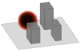
Refer to caption
Refer to caption
Refer to caption
Fig. 3: Volume renderings of the time evolution of u𝑢u for the three-dimensional model problem. The initial condition m𝑚m is shown in the left, and the middle and right images correspond to snapshots at times t=1𝑡1t=1 and t=2𝑡2t=2.

The observation operator \mathcal{B} then extracts the values of u𝑢u on a set of sensor locations {𝒙1,,𝒙Ns}𝒟subscript𝒙1subscript𝒙subscript𝑁𝑠𝒟\{{\mathchoice{\mbox{\boldmath$\displaystyle{x}$}}{\mbox{\boldmath$\textstyle{x}$}}{\mbox{\boldmath$\scriptstyle{x}$}}{\mbox{\boldmath$\scriptscriptstyle{x}$}}}_{1},\ldots,{\mathchoice{\mbox{\boldmath$\displaystyle{x}$}}{\mbox{\boldmath$\textstyle{x}$}}{\mbox{\boldmath$\scriptstyle{x}$}}{\mbox{\boldmath$\scriptscriptstyle{x}$}}}_{N_{s}}\}\subset\mathcal{D} at times {τ1,,τNτ}[0,T]subscript𝜏1subscript𝜏subscript𝑁𝜏0𝑇\{\tau_{1},\ldots,\tau_{N_{\tau}}\}\subset[0,T]. To summarize, the infinite-dimensional linear parameter-to-observable map \mathcal{F} maps the initial condition m𝑚m to q=NsNτ𝑞subscript𝑁𝑠subscript𝑁𝜏q={N_{s}}{N_{\tau}} observations as follows: First, we solve the time-dependent advection-diffusion equation (24), resulting in the space-time solution u=u(m)𝑢𝑢𝑚u=u(m). Then, the observation operator extracts point values from u𝑢u at the measurement locations and times, i.e., evaluates u𝑢\mathcal{B}u. The corresponding discrete parameter-to-observable map 𝐅𝐅\mathbf{F} is obtained by discretizing m𝑚m and u𝑢u using, for instance, finite elements.

5.2 The Bayesian inverse problem

Following the Bayesian setup in Section 2.1, we utilize a Gaussian prior measure μ0=𝒩(m0,𝒞0)subscript𝜇0𝒩subscript𝑚0subscript𝒞0\mu_{0}=\mathcal{N}\left(m_{0},\mathcal{C}_{0}\right), with 𝒞0=𝒜2subscript𝒞0superscript𝒜2\mathcal{C}_{0}=\mathcal{A}^{-2} where 𝒜𝒜\mathcal{A} is an elliptic differential operator as described in Section 2.1, and use an additive Gaussian noise model. Therefore, the solution of the Bayesian inverse problem is the posterior measure, μpost=𝒩(mpost,𝒞post)subscript𝜇post𝒩subscript𝑚postsubscript𝒞post\mu_{\rm{post}}=\mathcal{N}\left(m_{\text{post}},\mathcal{C}_{\text{post}}\right) with mpostsubscript𝑚postm_{\text{post}} and 𝒞postsubscript𝒞post\mathcal{C}_{\text{post}} as given in (5). The posterior mean mpostsubscript𝑚postm_{\text{post}} is characterized as the minimizer of

𝒥(m):=12u(m)𝒅Γnoise12+12𝒜(mm0)L2(𝒟)2,assign𝒥𝑚12subscriptsuperscriptnorm𝑢𝑚𝒅2subscriptsuperscriptΓ1noise12subscriptsuperscriptnorm𝒜𝑚subscript𝑚02superscript𝐿2𝒟\displaystyle\mathcal{J}(m):=\frac{1}{2}\left\|\mathcal{B}u(m)-{\mathchoice{\mbox{\boldmath$\displaystyle{d}$}}{\mbox{\boldmath$\textstyle{d}$}}{\mbox{\boldmath$\scriptstyle{d}$}}{\mbox{\boldmath$\scriptscriptstyle{d}$}}}\right\|^{2}_{\Gamma^{-1}_{\mathrm{noise}}}+\frac{1}{2}\left\|\mathcal{A}(m-m_{0}\right)\|^{2}_{L^{2}(\mathcal{D})},

which can also be interpreted as the regularized functional to be minimized in deterministic inversion. Next, we specify the action of the adjoint superscript\mathcal{F}^{*} of the parameter-to-observable map. Given an observation vector 𝒅¯qbold-¯𝒅superscript𝑞{\mathchoice{\mbox{\boldmath$\displaystyle{\bar{d}}$}}{\mbox{\boldmath$\textstyle{\bar{d}}$}}{\mbox{\boldmath$\scriptstyle{\bar{d}}$}}{\mbox{\boldmath$\scriptscriptstyle{\bar{d}}$}}}\in\mathbb{R}^{q} as defined in (13), 𝒅¯superscriptbold-¯𝒅\mathcal{F}^{*}{\mathchoice{\mbox{\boldmath$\displaystyle{\bar{d}}$}}{\mbox{\boldmath$\textstyle{\bar{d}}$}}{\mbox{\boldmath$\scriptstyle{\bar{d}}$}}{\mbox{\boldmath$\scriptscriptstyle{\bar{d}}$}}} is computed by solving the adjoint equation (see [1, 14, 29]) for the adjoint variable p=p(𝒙,t)𝑝𝑝𝒙𝑡p=p({\mathchoice{\mbox{\boldmath$\displaystyle{x}$}}{\mbox{\boldmath$\textstyle{x}$}}{\mbox{\boldmath$\scriptstyle{x}$}}{\mbox{\boldmath$\scriptscriptstyle{x}$}}},t),

pt(p𝒗)κΔpsubscript𝑝𝑡𝑝𝒗𝜅Δ𝑝\displaystyle-p_{t}-\nabla\cdot(p{\mathchoice{\mbox{\boldmath$\displaystyle{v}$}}{\mbox{\boldmath$\textstyle{v}$}}{\mbox{\boldmath$\scriptstyle{v}$}}{\mbox{\boldmath$\scriptscriptstyle{v}$}}})-\kappa\Delta p =𝒅¯absentsuperscriptbold-¯𝒅\displaystyle=-\mathcal{B}^{*}{\mathchoice{\mbox{\boldmath$\displaystyle{\bar{d}}$}}{\mbox{\boldmath$\textstyle{\bar{d}}$}}{\mbox{\boldmath$\scriptstyle{\bar{d}}$}}{\mbox{\boldmath$\scriptscriptstyle{\bar{d}}$}}} in 𝒟×(0,T),in 𝒟0𝑇\displaystyle\text{ in }\mathcal{D}\times(0,T), (26)
p(,T)𝑝𝑇\displaystyle p(\cdot,T) =0absent0\displaystyle=0 in 𝒟,in 𝒟\displaystyle\text{ in }\mathcal{D},
(𝒗p+κp)𝒏𝒗𝑝𝜅𝑝𝒏\displaystyle({\mathchoice{\mbox{\boldmath$\displaystyle{v}$}}{\mbox{\boldmath$\textstyle{v}$}}{\mbox{\boldmath$\scriptstyle{v}$}}{\mbox{\boldmath$\scriptscriptstyle{v}$}}}p+\kappa\nabla p)\cdot{\mathchoice{\mbox{\boldmath$\displaystyle{n}$}}{\mbox{\boldmath$\textstyle{n}$}}{\mbox{\boldmath$\scriptstyle{n}$}}{\mbox{\boldmath$\scriptscriptstyle{n}$}}} =0absent0\displaystyle=0 on 𝒟×(0,T),on 𝒟0𝑇\displaystyle\text{ on }\partial\mathcal{D}\times(0,T),

and setting 𝒅¯=p(,0)superscriptbold-¯𝒅𝑝0\mathcal{F}^{*}{\mathchoice{\mbox{\boldmath$\displaystyle{\bar{d}}$}}{\mbox{\boldmath$\textstyle{\bar{d}}$}}{\mbox{\boldmath$\scriptstyle{\bar{d}}$}}{\mbox{\boldmath$\scriptscriptstyle{\bar{d}}$}}}=p(\cdot,0). Note that (26) is a final value problem, which has to be solved backwards in time.

5.3 Discretization and solvers

The discretization of the forward and adjoint problems uses linear triangular/tetrahedral continuous Galerkin finite elements for two/three space dimensions, and the implicit Euler method in time. The discrete adjoint equation is obtained as the adjoint of the discretized forward equation, i.e., we follow a discretize-then-optimize approach. Due to the large diffusion parameter κ𝜅\kappa used, no stabilization of the advection-diffusion equation is needed. A factorization of the matrix in each implicit Euler time step is computed upfront, such that every time step (of the forward as well as the adjoint equation) only requires triangular solves.

The OED optimization problems are solved using Matlab’s built-in interior-point solver fmincon, to which we supply the OED objective function evaluation and its derivative, which we compute using the methods presented above. The optimization algorithm approximates second derivatives using the Broyden-Fletcher-Goldfarb-Shanno (BFGS) [27] method.

6 Numerical results

In this section, we summarize our numerical experiments. In Section 6.1, we provide a detailed numerical study of our method and compare different sparsifications for the two-dimensional model problem. Then, in Section 6.2, we use the three-dimensional model problem to test the scalability and performance of our OED method.

6.1 The two-dimensional model problem

This section contains numerical experiments for the two-dimensional model problem. We use Ns=122subscript𝑁𝑠122{N_{s}}=122 candidate locations for placing sensors as shown in Figure 2(b), and use 186418641864 triangles to discretize the domain. Linear finite elements are used for the parameter m𝑚m and the state variable u𝑢u resulting in n=1012𝑛1012{n}=1012 spatial degrees of freedom (and thus inversion parameters). The final time is T=4𝑇4T=4 and the time interval is discretized using Nt+1subscript𝑁𝑡1{N_{t}}+1 implicit Euler time steps; unless otherwise specified, Nt=64subscript𝑁𝑡64{N_{t}}=64. Observations at the sensor locations are taken at Nτ=19subscript𝑁𝜏19{N_{\tau}}=19 equally spaced points in the time interval [1,4]14[1,4]. The prior covariance is specified as described in Section 2.1 with α=8×10³𝛼8superscript103\alpha=8\times 10^{-3} and β=102𝛽superscript102\beta=10^{-2}; these values result in a Gaussian prior that is not overly restrictive or smoothing. Next, we study the low-rank approximations of the forward operator and the misfit Hessian.

6.1.1 Low-rank approximation of 𝐅𝐅\mathbf{F}, 𝐅~~𝐅\mathbf{\tilde{F}} and 𝐇misfitsubscript𝐇misfit\mathbf{H}_{\text{misfit}}

We use a randomized SVD to compute a low-rank surrogate for the parameter-to-observable map 𝐅:nq:𝐅superscript𝑛superscript𝑞\mathbf{F}:\mathbb{R}^{n}\to\mathbb{R}^{q} and its prior-preconditioned counterpart 𝐅~~𝐅\mathbf{\tilde{F}}, where q=Ns×Nτ𝑞subscript𝑁𝑠subscript𝑁𝜏q={N_{s}}\times{N_{\tau}}. This directly leads to a low-rank approximation of the prior-preconditioned misfit Hessian, 𝐇~misfit(𝒘)=𝐅~𝐖𝐅~subscript~𝐇misfit𝒘superscript~𝐅𝐖~𝐅\mathbf{\tilde{H}}_{\text{misfit}}({\mathchoice{\mbox{\boldmath$\displaystyle{w}$}}{\mbox{\boldmath$\textstyle{w}$}}{\mbox{\boldmath$\scriptstyle{w}$}}{\mbox{\boldmath$\scriptscriptstyle{w}$}}})=\mathbf{\tilde{F}}^{*}\mathbf{{W}}\mathbf{\tilde{F}}, where the diagonal weight matrix 𝐖𝐖\mathbf{{W}} depends on the design. Since the diagonal entries of 𝐖𝐖\mathbf{{W}} may vanish, the numerical rank of 𝐇~misfit(𝒘)subscript~𝐇misfit𝒘\mathbf{\tilde{H}}_{\text{misfit}}({\mathchoice{\mbox{\boldmath$\displaystyle{w}$}}{\mbox{\boldmath$\textstyle{w}$}}{\mbox{\boldmath$\scriptstyle{w}$}}{\mbox{\boldmath$\scriptscriptstyle{w}$}}}) is less than or equal than that of 𝐅~𝐅~superscript~𝐅~𝐅\mathbf{\tilde{F}}^{*}\mathbf{\tilde{F}}, which corresponds to assigning unit weights to all sensors; thus, it suffices to examine the accuracy of the approximation of 𝐇~misfit=𝐅~𝐅~subscript~𝐇misfitsuperscript~𝐅~𝐅\mathbf{\tilde{H}}_{\text{misfit}}=\mathbf{\tilde{F}}^{*}\mathbf{\tilde{F}} only.

First, we study the low-rank approximation of the (prior-preconditioned) parameter-to-observable map. In Figure 4 (left), we show the normalized singular values of 𝐅~~𝐅\mathbf{\tilde{F}} and of 𝐅𝐅{\mathbf{F}}. The eigenvalues decay rapidly and thus both mappings can be accurately approximated by low-rank matrices. Note the faster decay of the singular values of 𝐅~~𝐅\mathbf{\tilde{F}} compared to those of 𝐅𝐅{\mathbf{F}}, which shows that due to the preconditioning with 𝚪prior1/2superscriptsubscript𝚪prior12\boldsymbol{\Gamma}_{\rm{prior}}^{1/2}, 𝐅~~𝐅\mathbf{\tilde{F}} can be approximated more efficiently with a low-rank operator than 𝐅𝐅{\mathbf{F}}.

100superscript10010^{0}101superscript10110^{1}102superscript10210^{2}108superscript10810^{-8}105superscript10510^{-5}102superscript10210^{-2}101superscript10110^{1}k𝑘kσk/σ1subscript𝜎𝑘subscript𝜎1\sigma_{k}/\sigma_{1}spectrum of 𝐅𝐅\mathbf{F}spectrum of 𝐅~~𝐅\tilde{\mathbf{F}}
00505050100100100150150150200200200104superscript10410^{-4}100superscript10010^{0}104superscript10410^{4}108superscript10810^{8}k𝑘kλksubscript𝜆𝑘\lambda_{k}n=507,Nt=64formulae-sequence𝑛507subscript𝑁𝑡64n=507,N_{t}=64n=1012,Nt=64formulae-sequence𝑛1012subscript𝑁𝑡64n=1012,N_{t}=64n=1012,Nt=128formulae-sequence𝑛1012subscript𝑁𝑡128n=1012,N_{t}=128n=2036,Nt=64formulae-sequence𝑛2036subscript𝑁𝑡64n=2036,N_{t}=64
Fig. 4: Shown on the left are the normalized singular values of 𝐅~~𝐅\mathbf{\tilde{F}} and 𝐅𝐅\mathbf{F}. The right plot depicts the spectrum of the prior-preconditioned misfit Hessian with unit sensor weights 𝐇~misfit=𝐅~𝐅~subscript~𝐇misfitsuperscript~𝐅~𝐅\mathbf{\tilde{H}}_{\text{misfit}}=\mathbf{\tilde{F}}^{*}\mathbf{\tilde{F}} for discretizations with different numbers n𝑛n of spatial and Ntsubscript𝑁𝑡{N_{t}} of temporal unknowns. To compute these spectra, we used a rank r=500𝑟500r=500 approximation 𝐅~rsubscript~𝐅𝑟\mathbf{\tilde{F}}_{r} to diminish the influence of the low-rank approximation for 𝐅~~𝐅\mathbf{\tilde{F}}.

Next, we investigate the influence of spatial and temporal discretization on the prior-preconditioned misfit Hessian; the right plot in Figure 4 shows the eigenvalues of 𝐇~misfitsubscript~𝐇misfit\mathbf{\tilde{H}}_{\text{misfit}} for different spatial and temporal discretizations. Note that the spectra lie almost on top of each other. This indicates that the discretizations 𝐇~misfitsubscript~𝐇misfit\mathbf{\tilde{H}}_{\text{misfit}} converge to their infinite-dimensional counterpart, ~misfit:L2(𝒟)L2(𝒟):subscript~misfitsuperscript𝐿2𝒟superscript𝐿2𝒟\mathcal{\tilde{H}}_{\text{misfit}}:L^{2}(\mathcal{D})\to L^{2}(\mathcal{D}) and that all discretizations studied in Figure 4 resolve the dominant physics of the problem.

Finally, we study how the number of candidate sensor locations affects the spectral decay of 𝐅~~𝐅\mathbf{\tilde{F}}. Increasing the number of sensors has the potential to increases the information in the data and thus the numerical rank of 𝐅~~𝐅\mathbf{\tilde{F}}. In Figure 5, we plot the singular values of 𝐅~~𝐅\mathbf{\tilde{F}} for different sensor grids. We observe convergence of the singular value curves as the sensor grids are refined. This is a consequence of the correlation of the information that can be gained from neighboring sensors, which is due to the diffusion term in (24).

002002002004004004001010superscript101010^{-10}106superscript10610^{-6}102superscript10210^{-2}102superscript10210^{2}k𝑘kσksubscript𝜎𝑘\sigma_{k}Ns=33subscript𝑁𝑠33{N_{s}}=33Ns=58subscript𝑁𝑠58{N_{s}}=58Ns=85subscript𝑁𝑠85{N_{s}}=85Ns=122subscript𝑁𝑠122{N_{s}}=122Ns=216subscript𝑁𝑠216{N_{s}}=216Ns=407subscript𝑁𝑠407{N_{s}}=407
Fig. 5: Singular values of 𝐅~~𝐅\mathbf{\tilde{F}} for different values of Nssubscript𝑁𝑠{N_{s}}. The results correspond to a discretization of the problem with parameter dimension n=1012𝑛1012{n}=1012 and Nt=26subscript𝑁𝑡superscript26{N_{t}}=2^{6} time steps.

6.1.2 A-optimal designs with 1subscript1\ell_{1}-sparsification

We now apply our method to compute 1subscript1\ell_{1}-sparsified A-optimal designs. The weights 𝒘𝒘\textstyle{w} found with γ=6×101γ6superscript101\upgamma=6\times 10^{1} are shown in Figure 6 (left). As discussed in Section 4.5, sensors are then placed at locations corresponding to non-vanishing weights. To account for numerical errors introduced by the interior point method used to solve (12), non-vanishing weights are defined as weights wisubscript𝑤𝑖w_{i} that satisfy wi/jwj>4×103subscript𝑤𝑖subscript𝑗subscript𝑤𝑗4superscript103{w_{i}}/{\sum_{j}w_{j}}>4\times 10^{-3}; the resulting sensor locations are shown in Figure 6 (right). Next, we study the behavior of our method for computing 1subscript1\ell_{1}-sparsified designs.

Refer to captionRefer to captionx𝑥xy𝑦yx𝑥xy𝑦y
Fig. 6: Shown on the left are the weights found by solving the optimization problem (12) with 1subscript1\ell_{1}-sparsification. The right image shows the optimal sensor locations (black dots) obtained by placing sensors at locations with non-vanishing weights. Also shown is the advective flow field 𝒗𝒗\textstyle{v} (red arrows).

Since we rely on a low-rank surrogate 𝐅~rsubscript~𝐅𝑟\mathbf{\tilde{F}}_{r} for the prior-preconditioned parameter-to-observable map 𝐅~~𝐅\mathbf{\tilde{F}} to avoid repeated PDE solves in the OED method, we first examine the influence of this truncation on the optimal design. For that purpose, we fix γ=5×101γ5superscript101\upgamma=5\times 10^{1} and solve the A-optimal design problem using approximations 𝐅~rsubscript~𝐅𝑟\mathbf{\tilde{F}}_{r} with r=10,15,20,30,40,60,80𝑟10152030406080r=10,15,20,30,40,60,80. In Figure 7, we plot the optimal objective value Θ(𝒘opt)Θsubscript𝒘opt\Theta({\mathchoice{\mbox{\boldmath$\displaystyle{w}$}}{\mbox{\boldmath$\textstyle{w}$}}{\mbox{\boldmath$\scriptstyle{w}$}}{\mbox{\boldmath$\scriptscriptstyle{w}$}}}_{\text{opt}}) computed using low-rank surrogates 𝐅~rsubscript~𝐅𝑟\mathbf{\tilde{F}}_{r} with different r𝑟r. The convergence of the objective value shows that very similar results are found for low-rank surrogates 𝐅~rsubscript~𝐅𝑟\mathbf{\tilde{F}}_{r} with r40𝑟40r\geq 40. This shows that even a significant compression of the (preconditioned) parameter-to-observable map has little influence on the optimal design.

202020404040606060808080202020222222242424rank r𝑟r of surrogate 𝐅~rsubscript~𝐅𝑟\mathbf{\tilde{F}}_{r}Θ(𝒘opt)Θsubscript𝒘opt\Theta({\mathchoice{\mbox{\boldmath$\displaystyle{w}$}}{\mbox{\boldmath$\textstyle{w}$}}{\mbox{\boldmath$\scriptstyle{w}$}}{\mbox{\boldmath$\scriptscriptstyle{w}$}}}_{\text{opt}})
Param. dim. Iterations Func. eval.
517 82 153
1012 64 154
2036 77 165
3179 79 141
Fig. 7: Left: Value of Θ(𝒘opt)Θsubscript𝒘opt\Theta({\mathchoice{\mbox{\boldmath$\displaystyle{w}$}}{\mbox{\boldmath$\textstyle{w}$}}{\mbox{\boldmath$\scriptstyle{w}$}}{\mbox{\boldmath$\scriptscriptstyle{w}$}}}_{\text{opt}}) for an 1subscript1\ell_{1}-sparsified A-optimal design obtained with rank-r𝑟r approximations 𝐅~rsubscript~𝐅𝑟\mathbf{\tilde{F}}_{r}. Right: Number of interior-point quasi Newton iterations and function evaluations for different discretizations (and thus different parameter dimensions).

Next, we study the effect of increasing the parameter dimension (through mesh refinements) on the number of interior-point iterations required to solve the OED optimization problem (16). As observed in Section 6.1.1, increasing the parameter dimension does not increase the numerical rank of 𝐅~~𝐅\mathbf{\tilde{F}} once the mesh is sufficiently fine. This, and the use of a Newton-type optimization method results in a nearly constant number of interior-point iterations required to solve (16), as shown in the table in Figure 7.

Finally, we study how the performance of the numerical optimization encountered in our OED method is affected by increasing the number Nssubscript𝑁𝑠{N_{s}} of candidate sensor locations; note that Nssubscript𝑁𝑠{N_{s}} is also the dimension of the weight vector 𝒘𝒘\textstyle{w}, the unknown in the OED optimization problem (16). The results shown in Table 1 show that the number of interior-point quasi-Newton iterations and the number of evaluations of Θ()Θ\Theta(\cdot) do not increase significantly as the number of sensor candidate locations increases. We again attribute this to the use of a Newton-type method, since Newton’s method satisfies—under certain assumptions—a mesh independence property [12].

Table 1: Number of interior-point BFGS iterations and evaluations of Θ()Θ\Theta(\cdot) required for the solution of (16) with 1subscript1\ell_{1}-sparsification, for different numbers Nssubscript𝑁𝑠{N_{s}} of sensor candidate locations. The optimization iteration was terminated when the norm of the gradient was decreased by a factor of 104superscript10410^{4}.
Nssubscript𝑁𝑠{N_{s}} 333333 585858 858585 122122122 172172172 216216216 264264264 340340340
Iterations 585858 686868 686868 818181 585858 686868 757575 727272
Func. eval. 149149149 165165165 141141141 158158158 136136136 137137137 122122122 160160160

Regarding the complexity of our method with respect to the number Nssubscript𝑁𝑠{N_{s}} of candidate sensor locations, we draw the following conclusions from Figure 5 and Table 1: First, the number of PDE solves required to compute the low-rank surrogate 𝐅~rsubscript~𝐅𝑟\mathbf{\tilde{F}}_{r} is bounded with respect to Nssubscript𝑁𝑠{N_{s}}, and second, the number of optimization iterations to solve (16) is insensitive to the number of candidate sensor locations, and thus the dimension of the weight vector 𝒘𝒘\textstyle{w}.

6.1.3 A-optimal designs with ΦεsubscriptΦ𝜀\Phi_{\varepsilon}-sparsification

Next, we present ΦεsubscriptΦ𝜀\Phi_{\varepsilon}-sparsified designs obtained by a continuation procedure with respect to ε𝜀\varepsilon. Optimal designs for γ=0.05γ0.05\upgamma=0.05 and γ=0.06γ0.06\upgamma=0.06 are shown on the left in Figure 8. Note that the optimal sensor locations obtained with γ=0.06γ0.06\upgamma=0.06 is not a subset of the locations obtained with γ=0.05γ0.05\upgamma=0.05, i.e., the designs are not nested.

For the continuation procedure, we use the values εi=(2/3)isubscript𝜀𝑖superscript23𝑖\varepsilon_{i}=(2/3)^{i}, i=1,,10𝑖110i=1,\ldots,10. To elucidate the convergence of the weights to the desired binary structure, the weights corresponding to several values of εisubscript𝜀𝑖\varepsilon_{i} are shown on the right in Figure 8. Note that the behavior of the weights is not monotone as ε𝜀\varepsilon is decreased. A possible explanation for this behavior is that, as ε𝜀\varepsilon decreases, weights at neighboring locations can get merged into a single weight at a new location.
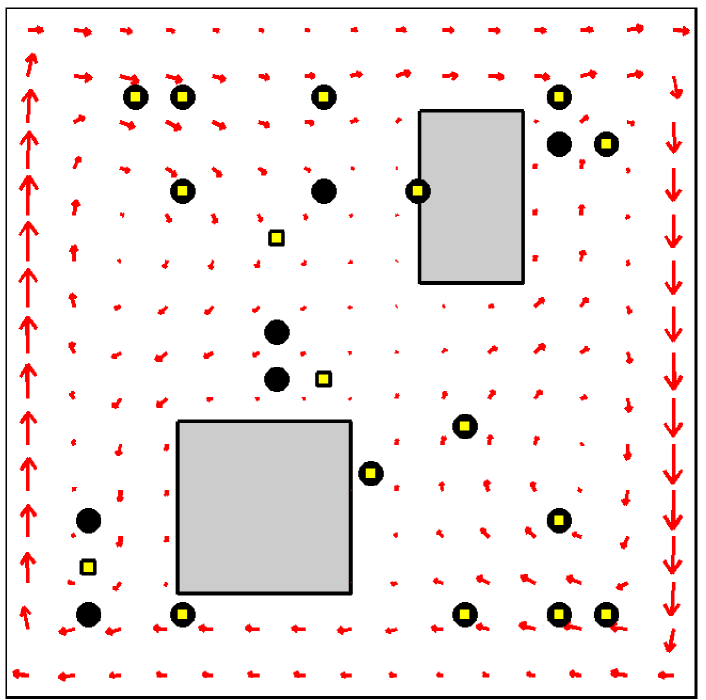
Refer to caption
505050100100100000.50.50.5111j𝑗jws(j)subscript𝑤𝑠𝑗w_{s(j)}ε1subscript𝜀1\varepsilon_{1}ε2subscript𝜀2\varepsilon_{2}ε4subscript𝜀4\varepsilon_{4}ε10subscript𝜀10\varepsilon_{10}
Fig. 8: Left: Sensor locations using ΦεsubscriptΦ𝜀\Phi_{\varepsilon}-sparsified A-optimal design for γ=0.05γ0.05\upgamma=0.05 (black dots) and for γ=0.06γ0.06\upgamma=0.06 (yellow squares). Right: Convergence of the weights to a 0–1 structure as ε0𝜀0\varepsilon\to 0. The weights are ordered based on the values obtained with ε1subscript𝜀1\varepsilon_{1}, and shown is the evolution of the weights as ε𝜀\varepsilon decreases. Here, s(j)𝑠𝑗s(j) denotes the descending ordering obtained with ε1subscript𝜀1\varepsilon_{1}.

To illustrate the decreased variance for A-optimal designs, in Figure 9 we compare the pointwise posterior standard deviation obtained with γ=0.05γ0.05\upgamma=0.05 with a uniform and two randomly generated designs employing the same number of sensors. This comparison shows that the A-optimal design provides a notable reduction in the standard deviation (and thus the variance) fields. Next, we compare the performance of sensor placements obtained with 1subscript1\ell_{1}- and ΦεsubscriptΦ𝜀\Phi_{\varepsilon}-sparsification.

Refer to caption
Refer to caption
Refer to caption
Refer to caption

(a) (b) (c) (d)             .

Fig. 9: Shown is the pointwise standard deviation of the posterior for a ΦεsubscriptΦ𝜀\Phi_{\varepsilon}-sparsified A-optimal design with 20 sensors (a), for a manually chosen uniform design (b), and two randomly generated designs with the same number of sensors (c), (d). The white dots indicate the sensor locations. Red and blue correspond to regions with large and small standard deviation, respectively. We find that compared to the optimal design, the uniform design and the two random designs result in 7%percent77\%, 36%percent3636\% and 26%percent2626\% increase in the average variance, respectively.

6.1.4 Comparing 1subscript1\ell_{1}- and ΦεsubscriptΦ𝜀\Phi_{\varepsilon}-sparsifications

We observe that 1subscript1\ell_{1}- and ΦεsubscriptΦ𝜀\Phi_{\varepsilon}-sparsifications lead to different designs for the same number of sensors. Thus, a naturally arising question is (1) which sparsification results in the better placement of sensors? Moreover, (2) how much do optimal designs improve over randomly chosen designs? To answer these questions, we compute optimal designs based on different sparsification strategies and compare with randomly generated designs. We use trace estimators with 100100100 Gaussian random vectors chosen differently in each OED problem, but report the exact value of 𝗍𝗋(𝚪post(𝒘))=𝗍𝗋(𝐇(𝒘)1)𝗍𝗋subscript𝚪post𝒘𝗍𝗋𝐇superscript𝒘1\mathsf{tr}(\mathbf{\Gamma}_{\text{post}}({\mathchoice{\mbox{\boldmath$\displaystyle{w}$}}{\mbox{\boldmath$\textstyle{w}$}}{\mbox{\boldmath$\scriptstyle{w}$}}{\mbox{\boldmath$\scriptscriptstyle{w}$}}}))=\mathsf{tr}(\mathbf{H}({\mathchoice{\mbox{\boldmath$\displaystyle{w}$}}{\mbox{\boldmath$\textstyle{w}$}}{\mbox{\boldmath$\scriptstyle{w}$}}{\mbox{\boldmath$\scriptscriptstyle{w}$}}})^{-1}).

Our results are summarized in Figure 11. We compute 1subscript1\ell_{1}-sparsified designs for various values of γγ\upgamma and report the value of 𝗍𝗋(𝐇(𝒘)1)𝗍𝗋𝐇superscript𝒘1\mathsf{tr}(\mathbf{H}({\mathchoice{\mbox{\boldmath$\displaystyle{w}$}}{\mbox{\boldmath$\textstyle{w}$}}{\mbox{\boldmath$\scriptstyle{w}$}}{\mbox{\boldmath$\scriptscriptstyle{w}$}}})^{-1}). Similarly, we report 𝗍𝗋(𝐇(𝒘)1)𝗍𝗋𝐇superscript𝒘1\mathsf{tr}(\mathbf{H}({\mathchoice{\mbox{\boldmath$\displaystyle{w}$}}{\mbox{\boldmath$\textstyle{w}$}}{\mbox{\boldmath$\scriptstyle{w}$}}{\mbox{\boldmath$\scriptscriptstyle{w}$}}})^{-1}) for 0–1 optimal designs computed via ΦεsubscriptΦ𝜀\Phi_{\varepsilon}-sparsification. Additionally, we compute 𝗍𝗋(𝐇(𝒘)1)𝗍𝗋𝐇superscript𝒘1\mathsf{tr}(\mathbf{H}({\mathchoice{\mbox{\boldmath$\displaystyle{w}$}}{\mbox{\boldmath$\textstyle{w}$}}{\mbox{\boldmath$\scriptstyle{w}$}}{\mbox{\boldmath$\scriptscriptstyle{w}$}}})^{-1}) for a collection of random sensor configurations. We find that ΦεsubscriptΦ𝜀\Phi_{\varepsilon}-sparsified designs consistently outperform 1subscript1\ell_{1}-sparsified designs and that both improve significantly over randomly chosen designs. Another observation from Figure 11 is the diminishing returns as the number of sensors is increased; using more than 202020 sensors only results in negligible decrease of the OED objective function value.

6.1.5 Influence of trace estimation

To assess the accuracy of randomized trace estimation for a typical posterior covariance matrix, we compare the exact trace with results from randomized trace estimation with different numbers of random vectors. We find that trace estimators based on 1, 5, 10, 20, 100 vectors estimate the exact trace with an average error of about 15%, 7%, 5%, 2% and 1.5%, respectively. This is consistent with the experiments reported in [3] showing that randomized trace estimation is reasonably accurate with a small number of random vectors, but that many random vectors may be needed to obtain very accurate approximations.

A more relevant question in the context of OED is how the use of trace estimators to compute optimal sensor locations influences the resulting designs. To study this issue, we compute optimal designs with fixed γγ\upgamma, but different trace estimators. The results are shown in Figure 10. Note that trace estimation in the OED objective function does have an influence on the designs. More accurate trace estimation decreases the variation in both the number of sensors of the designs and the value of the trace of the posterior covariance. However, as can be seen from Figure 11 optimal designs computed using trace estimation (based on 100 random vectors) consistently improve over random designs with respect to reducing the exact trace of the posterior covariance. We thus conclude that the use of trace estimation does not have a significant impact on the quality of the optimal designs.
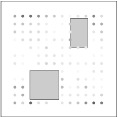
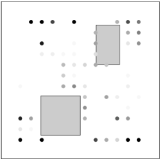
Refer to caption
Refer to caption
121212141414161616181818202020222222444555666777Number of sensors𝗍𝗋(𝚪post(𝒘))𝗍𝗋subscript𝚪post𝒘\mathsf{tr}(\boldsymbol{\Gamma}_{\rm{post}}({\mathchoice{\mbox{\boldmath$\displaystyle{w}$}}{\mbox{\boldmath$\textstyle{w}$}}{\mbox{\boldmath$\scriptstyle{w}$}}{\mbox{\boldmath$\scriptscriptstyle{w}$}}}))N𝗍𝗋=1subscript𝑁𝗍𝗋1{N_{{\mathsf{tr}}}}=1N𝗍𝗋=100subscript𝑁𝗍𝗋100{N_{{\mathsf{tr}}}}=100
Fig. 10: Sensitivity of ΦεsubscriptΦ𝜀\Phi_{\varepsilon}-sparsified designs with respect to the trace estimator with fixed γ=0.05γ0.05\upgamma=0.05. The left and the middle image visualize the frequency of a candidate location being part of the optimal design with a trace estimator based on a single random vector (left) and 100 random vectors (middle). The results are based on 30 different realizations of the respective trace estimators. The darker the candidate location, the more often the corresponding sensor was part of the optimal design. Note the decreased variation in the designs in the middle plot, which is due to the increased accuracy of the trace estimator. The right plot depicts the number of sensors and the value of the trace of the posterior covariance for 30 different trace estimators with a single random vector (empty dots) and with 100 random vectors (filled dots). Note that the number of sensors varies for the different realizations and that the more accurate trace estimator results in less scattering with respect to the number of sensors and the value of the trace.
00101010202020303030404040505050606060444666888101010121212Number of sensorstr(𝚪post(𝒘)subscript𝚪post𝒘\mathbf{\Gamma}_{\text{post}}({\mbox{\boldmath$\displaystyle{w}$}}))Random designs1subscript1\ell_{1}-sparsified designsΦεsubscriptΦ𝜀\Phi_{\varepsilon}-sparsified designs
Fig. 11: Comparison of performance for different designs. Shown is the value of 𝗍𝗋(𝐇1)𝗍𝗋superscript𝐇1\mathsf{tr}(\mathbf{H}^{-1}) versus the number of sensors for random designs (red dots), 1subscript1\ell_{1}-sparsified designs (cyan dots) and ΦεsubscriptΦ𝜀\Phi_{\varepsilon}-sparsified designs (black dots).

6.2 The three-dimensional model problem

The main target of this three dimensional model problem is to study the applicability of our OED method to large-scale inverse problems. The computational domain used is depicted in Figure 2(c), where 101101101 candidate sensor locations are shown as black dots. Note that we allow sensors on the ground and on the sides of the buildings. Observations are collected at Nτ=12subscript𝑁𝜏12{N_{\tau}}=12 equally spaced points in the time interval [1,T]1𝑇[1,T], where T=4𝑇4T=4. The parameter and the state variable u𝑢u in the advection-diffusion equation are discretized using linear finite elements on a tetrahedral mesh with 10,6521065210{,}652 spatial degrees of freedom, and 646464 implicit Euler time steps are used for the time integration. Thus, the dimension of the inversion parameter is n=10,652𝑛10652{n}=10{,}652.

Refer to caption
Refer to caption
Refer to caption
Refer to caption
Fig. 12: Top row: Sensor locations (black dots) obtained with A-optimal design with ΦεsubscriptΦ𝜀\Phi_{\varepsilon}-sparsification (left) and with random design (right). Bottom row: Standard deviation fields of the posterior for an A-optimal design with ΦεsubscriptΦ𝜀\Phi_{\varepsilon}-sparsification (left) and random design (right). Here, red indicates regions with large standard deviation, and blue corresponds to regions with small standard deviation.

In our computations, we found a rank-100100100 SVD surrogate for the prior-preconditioned parameter-to-observable map adequate since the 100100100th singular value of 𝐅~~𝐅\mathbf{\tilde{F}} is about four orders of magnitude smaller than the largest singular value. This translates to eight orders of magnitude difference between the first and the 100100100th eigenvalue of 𝐇~misfitsubscript~𝐇misfit\mathbf{\tilde{H}}_{\text{misfit}}. Due to the large parameter space dimension we do not compute 𝐌1/2superscript𝐌12{\mathbf{M}}^{-1/2} explicitly, but use the algorithm for the iterative application of 𝐌1/2superscript𝐌12{\mathbf{M}}^{-1/2} to vectors from [11]; see also Section 4.4. We observe that the algorithm is well converged after 101010 applications of 𝐌~~𝐌\tilde{{\mathbf{M}}}—the relative difference between the iterative application of 𝐌~1/2superscript~𝐌12\tilde{{\mathbf{M}}}^{-1/2} based on 101010 applications of 𝐌~~𝐌\tilde{{\mathbf{M}}} compared with that based on 500500500 applications of 𝐌~~𝐌\tilde{{\mathbf{M}}} is approximately 8×1068superscript1068\times 10^{-6}. For the solution of the OED optimization problem with γ=1.2×101γ1.2superscript101\upgamma=1.2\times 10^{-1} and ΦεsubscriptΦ𝜀\Phi_{\varepsilon}-sparsification, the continuation procedure presented in Section 6.1.2 is used. To compute the initial 1subscript1\ell_{1}-sparsified weight vector 𝒘0superscript𝒘0{\mathchoice{\mbox{\boldmath$\displaystyle{w}$}}{\mbox{\boldmath$\textstyle{w}$}}{\mbox{\boldmath$\scriptstyle{w}$}}{\mbox{\boldmath$\scriptscriptstyle{w}$}}}^{0}, 18 interior-point iterations were necessary. This initialization was followed by 10 continuation steps using the penalties ΦεisubscriptΦsubscript𝜀𝑖\Phi_{\varepsilon_{i}}, with εi=(2/3)isubscript𝜀𝑖superscript23𝑖\varepsilon_{i}=(2/3)^{i}; each step required the solution of an auxiliary OED problem, which amounted to a total of 554554554 interior-point quasi-Newton iterations to arrive at a 0–1 design vector. The iteration for each of these auxiliary OED problems was terminated when the relative residual dropped below 104superscript10410^{-4} or a maximum of 150 iterations was reached. The number of quasi-Newton iterations in the continuation procedure can likely be decreased by incorporating the continuation procedure into the interior-point algorithm rather than solving an independent interior point problem for each εisubscript𝜀𝑖\varepsilon_{i}.

The resulting optimal design is shown in top left image of Figure 12; note that several sensors are placed on the top of buildings; these sensors help reduce the variance in the upper parts of the domain. To illustrate the effectiveness of the optimal design to reduce the variance, in Figure 12 we show a volume rendering of the pointwise posterior standard deviation obtained with the optimal design, and compare it with a rendering obtained with a randomly generated design that has the same number of sensors.

7 Concluding remarks

We have developed a structure-exploiting efficient numerical method for computing A-optimal experimental designs in infinite-dimensional Bayesian linear inverse problems governed by PDEs. Numerical experiments for the inversion of the initial condition in an advection-diffusion equation indicate that an optimal design can be computed at a cost, measured in forward PDE solves, that is independent of the parameter and candidate sensor dimensions. Moreover, we find that experimental designs obtained with regularized 0subscript0\ell_{0}-sparsification are consistently superior to designs obtained with 1subscript1\ell_{1}-sparsification, and significantly improve over uniform and random designs.

One limitation of the OED method we have presented is that it relies on linearity of the parameter-to-observable map and assumes Gaussian prior and noise distributions. However, the methods presented here are also applicable in situations where a nonlinear parameter-to-observable map can be well approximated by a linearization over the set of parameters that have significant posterior probability. Moreover, using Gaussian noise and prior distributions is common, particularly in infinite-dimensional inference problems. The computational efficiency of our methods depends on low-rank approximations of the preconditioned parameter-to-observable map, which rely on properties of the associated forward and observation operators. As a consequence of ill-posedness, many parameter-to-observable operators admit such low-rank approximations. Finally, our relaxation of the design problem using a continuous weight vector in combination with sparsification provides just indirect control of the number of sensors through the value of γγ\upgamma. However, this approach makes the combinatorial OED problem of optimal sensor placement computationally tractable.

Possible extensions of the present work include consideration of (1) alternative optimal experimental design criteria that are meaningful in infinite dimensions and (2) nonlinear parameter-to-observable maps. OED with nonlinear parameter-to-observable maps is particularly challenging as, in general, the posterior is non-Gaussian, the (linearization of the) parameter-to-observable map in general depends on the state, parameter, and data variables and thus its low-rank approximation cannot be computed a priori, optimal designs might not be unique even if the sparsifying penalty is convex, and the misfit Hessian depends on (usually unavailable) observations.

Acknowledgments

We would like to thank James Martin for providing us with an implementation of the algorithm in [11], which was used to compute the application of the inverse square root of the mass matrix.

Appendix A The mass-weighted trace estimator

The following basic result justifies the form of the randomized trace estimator for an 𝐌𝐌{\mathbf{M}}-symmetric matrix as defined in section 2.2. The proof given below adapts the arguments given in [3] regarding Gaussian trace estimators for symmetric linear mappings on the standard Euclidean inner product space.

Proposition 1.

Let 𝐀𝐀{\mathbf{A}} be an 𝐌𝐌{\mathbf{M}}-symmetric linear mapping on 𝐌nsubscriptsuperscript𝑛𝐌\mathbb{R}^{n}_{\mathbf{M}}, n1𝑛1n\geq 1. Suppose 𝐲𝐲\textstyle{y} is a random n𝑛n-vector with i.i.d. 𝒩(0,1)𝒩01\mathcal{N}\left(0,1\right)-entries, and let 𝐳=𝐌1/2𝐲𝐳superscript𝐌12𝐲{\mathchoice{\mbox{\boldmath$\displaystyle{z}$}}{\mbox{\boldmath$\textstyle{z}$}}{\mbox{\boldmath$\scriptstyle{z}$}}{\mbox{\boldmath$\scriptscriptstyle{z}$}}}={\mathbf{M}}^{-1/2}{\mathchoice{\mbox{\boldmath$\displaystyle{y}$}}{\mbox{\boldmath$\textstyle{y}$}}{\mbox{\boldmath$\scriptstyle{y}$}}{\mbox{\boldmath$\scriptscriptstyle{y}$}}}. Then, T(𝐀):=𝐳,𝐀𝐳Massign𝑇𝐀subscript𝐳𝐀𝐳MT({\mathbf{A}}):=\left\langle{{\mathchoice{\mbox{\boldmath$\displaystyle{z}$}}{\mbox{\boldmath$\textstyle{z}$}}{\mbox{\boldmath$\scriptstyle{z}$}}{\mbox{\boldmath$\scriptscriptstyle{z}$}}}},{{\mathbf{A}}{\mathchoice{\mbox{\boldmath$\displaystyle{z}$}}{\mbox{\boldmath$\textstyle{z}$}}{\mbox{\boldmath$\scriptstyle{z}$}}{\mbox{\boldmath$\scriptscriptstyle{z}$}}}}\right\rangle_{\!\scriptscriptstyle{\text{M}}} is an unbiased estimator for 𝗍𝗋(𝐀)𝗍𝗋𝐀\mathsf{tr}({\mathbf{A}}); that is, 𝖤{T(𝐀)}=𝗍𝗋(𝐀)𝖤𝑇𝐀𝗍𝗋𝐀\mathsf{E}\left\{{T({\mathbf{A}})}\right\}=\mathsf{tr}({\mathbf{A}}).

Proof.

Since 𝐀𝐀{\mathbf{A}} is 𝐌𝐌{\mathbf{M}}-symmetric, it admits a spectral decomposition, 𝐀=𝐕𝚲𝐕𝐀𝐕𝚲superscript𝐕{\mathbf{A}}={\mathbf{V}}\mathbf{\Lambda}{\mathbf{V}}^{*}, with 𝐕𝐕{\mathbf{V}} a matrix with 𝐌𝐌{\mathbf{M}}-orthogonal eigenvectors of 𝐀𝐀{\mathbf{A}} as its columns (i.e., 𝐕T𝐌𝐕=𝐈superscript𝐕𝑇𝐌𝐕𝐈{\mathbf{V}}^{T}{\mathbf{M}}{\mathbf{V}}={\mathbf{I}}) and 𝚲𝚲\mathbf{\Lambda} a diagonal matrix with real eigenvalues {λi}i=1nsuperscriptsubscriptsubscript𝜆𝑖𝑖1𝑛\{\lambda_{i}\}_{i=1}^{n} of 𝐀𝐀{\mathbf{A}} on its diagonal. Then,

𝖤{T(𝐀)}=𝖤{𝒛T𝐌𝐕𝚲𝐕𝒛}=𝖤{𝒚T𝐌1/2𝐕𝚲𝐕T𝐌1/2𝒚}=𝖤{𝒒T𝚲𝒒},𝖤𝑇𝐀𝖤superscript𝒛𝑇𝐌𝐕𝚲superscript𝐕𝒛𝖤superscript𝒚𝑇superscript𝐌12𝐕𝚲superscript𝐕𝑇superscript𝐌12𝒚𝖤superscript𝒒𝑇𝚲𝒒\displaystyle\mathsf{E}\left\{{T({\mathbf{A}})}\right\}=\mathsf{E}\left\{{{\mathchoice{\mbox{\boldmath$\displaystyle{z}$}}{\mbox{\boldmath$\textstyle{z}$}}{\mbox{\boldmath$\scriptstyle{z}$}}{\mbox{\boldmath$\scriptscriptstyle{z}$}}}^{T}{\mathbf{M}}{\mathbf{V}}\mathbf{\Lambda}{\mathbf{V}}^{*}{\mathchoice{\mbox{\boldmath$\displaystyle{z}$}}{\mbox{\boldmath$\textstyle{z}$}}{\mbox{\boldmath$\scriptstyle{z}$}}{\mbox{\boldmath$\scriptscriptstyle{z}$}}}}\right\}=\mathsf{E}\left\{{{\mathchoice{\mbox{\boldmath$\displaystyle{y}$}}{\mbox{\boldmath$\textstyle{y}$}}{\mbox{\boldmath$\scriptstyle{y}$}}{\mbox{\boldmath$\scriptscriptstyle{y}$}}}^{T}{\mathbf{M}}^{1/2}{\mathbf{V}}\mathbf{\Lambda}{\mathbf{V}}^{T}{\mathbf{M}}^{1/2}{\mathchoice{\mbox{\boldmath$\displaystyle{y}$}}{\mbox{\boldmath$\textstyle{y}$}}{\mbox{\boldmath$\scriptstyle{y}$}}{\mbox{\boldmath$\scriptscriptstyle{y}$}}}}\right\}=\mathsf{E}\left\{{{\mathchoice{\mbox{\boldmath$\displaystyle{q}$}}{\mbox{\boldmath$\textstyle{q}$}}{\mbox{\boldmath$\scriptstyle{q}$}}{\mbox{\boldmath$\scriptscriptstyle{q}$}}}^{T}\mathbf{\Lambda}{\mathchoice{\mbox{\boldmath$\displaystyle{q}$}}{\mbox{\boldmath$\textstyle{q}$}}{\mbox{\boldmath$\scriptstyle{q}$}}{\mbox{\boldmath$\scriptscriptstyle{q}$}}}}\right\},

with 𝒒=𝐕T𝐌1/2𝒚𝒒superscript𝐕𝑇superscript𝐌12𝒚{\mathchoice{\mbox{\boldmath$\displaystyle{q}$}}{\mbox{\boldmath$\textstyle{q}$}}{\mbox{\boldmath$\scriptstyle{q}$}}{\mbox{\boldmath$\scriptscriptstyle{q}$}}}={\mathbf{V}}^{T}{\mathbf{M}}^{1/2}{\mathchoice{\mbox{\boldmath$\displaystyle{y}$}}{\mbox{\boldmath$\textstyle{y}$}}{\mbox{\boldmath$\scriptstyle{y}$}}{\mbox{\boldmath$\scriptscriptstyle{y}$}}}; note that above we also used 𝐕=𝐕T𝐌superscript𝐕superscript𝐕𝑇𝐌{\mathbf{V}}^{*}={\mathbf{V}}^{T}{\mathbf{M}}. It is straightforward to show that 𝒒𝒩(𝟎,𝐈)similar-to𝒒𝒩0𝐈{\mathchoice{\mbox{\boldmath$\displaystyle{q}$}}{\mbox{\boldmath$\textstyle{q}$}}{\mbox{\boldmath$\scriptstyle{q}$}}{\mbox{\boldmath$\scriptscriptstyle{q}$}}}\sim\mathcal{N}\left({\mathchoice{\mbox{\boldmath$\displaystyle{0}$}}{\mbox{\boldmath$\textstyle{0}$}}{\mbox{\boldmath$\scriptstyle{0}$}}{\mbox{\boldmath$\scriptscriptstyle{0}$}}},{\mathbf{I}}\right). Therefore,

𝖤{T(𝐀)}=𝖤{𝒒T𝚲𝒒}=i=1nλi𝖤{qi2}=i=1nλi=𝗍𝗋(𝐀),𝖤𝑇𝐀𝖤superscript𝒒𝑇𝚲𝒒superscriptsubscript𝑖1𝑛subscript𝜆𝑖𝖤superscriptsubscript𝑞𝑖2superscriptsubscript𝑖1𝑛subscript𝜆𝑖𝗍𝗋𝐀\mathsf{E}\left\{{T({\mathbf{A}})}\right\}=\mathsf{E}\left\{{{\mathchoice{\mbox{\boldmath$\displaystyle{q}$}}{\mbox{\boldmath$\textstyle{q}$}}{\mbox{\boldmath$\scriptstyle{q}$}}{\mbox{\boldmath$\scriptscriptstyle{q}$}}}^{T}\mathbf{\Lambda}{\mathchoice{\mbox{\boldmath$\displaystyle{q}$}}{\mbox{\boldmath$\textstyle{q}$}}{\mbox{\boldmath$\scriptstyle{q}$}}{\mbox{\boldmath$\scriptscriptstyle{q}$}}}}\right\}=\sum_{i=1}^{n}\lambda_{i}\mathsf{E}\left\{{q_{i}^{2}}\right\}=\sum_{i=1}^{n}\lambda_{i}=\mathsf{tr}({\mathbf{A}}),

where the penultimate equality follows from the fact that 𝖤{qi2}=1𝖤superscriptsubscript𝑞𝑖21\mathsf{E}\left\{{q_{i}^{2}}\right\}=1, which is the case because qi2superscriptsubscript𝑞𝑖2q_{i}^{2} is the square of standard normal random variable and is thus χ2superscript𝜒2\chi^{2} distributed with one degree of freedom. ∎

Appendix B Relation between the trace of posterior covariance and the expected MSE of the posterior mean

Here, we show that

nq𝒎post𝒅𝒎𝐌2𝑑μ𝒅|𝒎(𝒅)𝑑μ0(𝒎)=𝗍𝗋(𝚪post),subscriptsuperscript𝑛subscriptsuperscript𝑞subscriptsuperscriptnormsuperscriptsubscript𝒎post𝒅𝒎2𝐌differential-dsubscript𝜇conditional𝒅𝒎𝒅differential-dsubscript𝜇0𝒎𝗍𝗋subscript𝚪post\int_{\mathbb{R}^{n}}\int_{\mathbb{R}^{q}}\left\|{{\mathchoice{\mbox{\boldmath$\displaystyle{m}$}}{\mbox{\boldmath$\textstyle{m}$}}{\mbox{\boldmath$\scriptstyle{m}$}}{\mbox{\boldmath$\scriptscriptstyle{m}$}}}_{\text{post}}^{\mathchoice{\mbox{\boldmath$\displaystyle{d}$}}{\mbox{\boldmath$\textstyle{d}$}}{\mbox{\boldmath$\scriptstyle{d}$}}{\mbox{\boldmath$\scriptscriptstyle{d}$}}}-{\mathchoice{\mbox{\boldmath$\displaystyle{m}$}}{\mbox{\boldmath$\textstyle{m}$}}{\mbox{\boldmath$\scriptstyle{m}$}}{\mbox{\boldmath$\scriptscriptstyle{m}$}}}}\right\|^{2}_{\mathbf{M}}\,d\mu_{{\mathchoice{\mbox{\boldmath$\displaystyle{d}$}}{\mbox{\boldmath$\textstyle{d}$}}{\mbox{\boldmath$\scriptstyle{d}$}}{\mbox{\boldmath$\scriptscriptstyle{d}$}}}|{\mathchoice{\mbox{\boldmath$\displaystyle{m}$}}{\mbox{\boldmath$\textstyle{m}$}}{\mbox{\boldmath$\scriptstyle{m}$}}{\mbox{\boldmath$\scriptscriptstyle{m}$}}}}({\mathchoice{\mbox{\boldmath$\displaystyle{d}$}}{\mbox{\boldmath$\textstyle{d}$}}{\mbox{\boldmath$\scriptstyle{d}$}}{\mbox{\boldmath$\scriptscriptstyle{d}$}}})\,d\mu_{0}({\mathchoice{\mbox{\boldmath$\displaystyle{m}$}}{\mbox{\boldmath$\textstyle{m}$}}{\mbox{\boldmath$\scriptstyle{m}$}}{\mbox{\boldmath$\scriptscriptstyle{m}$}}})=\mathsf{tr}(\boldsymbol{\Gamma}_{\rm{post}}), (27)

where, according to our choice of the noise model, μ𝒅|𝒎=𝒩(𝐅𝒎,𝚪noise)subscript𝜇conditional𝒅𝒎𝒩𝐅𝒎subscript𝚪noise\mu_{{\mathchoice{\mbox{\boldmath$\displaystyle{d}$}}{\mbox{\boldmath$\textstyle{d}$}}{\mbox{\boldmath$\scriptstyle{d}$}}{\mbox{\boldmath$\scriptscriptstyle{d}$}}}|{\mathchoice{\mbox{\boldmath$\displaystyle{m}$}}{\mbox{\boldmath$\textstyle{m}$}}{\mbox{\boldmath$\scriptstyle{m}$}}{\mbox{\boldmath$\scriptscriptstyle{m}$}}}}=\mathcal{N}\left(\mathbf{F}{\mathchoice{\mbox{\boldmath$\displaystyle{m}$}}{\mbox{\boldmath$\textstyle{m}$}}{\mbox{\boldmath$\scriptstyle{m}$}}{\mbox{\boldmath$\scriptscriptstyle{m}$}}},\boldsymbol{\Gamma}_{\rm{noise}}\right) and μ0subscript𝜇0\mu_{0} is the (discretized) prior measure over 𝐌nsubscriptsuperscript𝑛𝐌\mathbb{R}^{n}_{\mathbf{M}}, μ0=𝒩(𝒎0,𝚪prior)subscript𝜇0𝒩subscript𝒎0subscript𝚪prior\mu_{0}=\mathcal{N}\left({\mathchoice{\mbox{\boldmath$\displaystyle{m}$}}{\mbox{\boldmath$\textstyle{m}$}}{\mbox{\boldmath$\scriptstyle{m}$}}{\mbox{\boldmath$\scriptscriptstyle{m}$}}}_{0},\boldsymbol{\Gamma}_{\rm{prior}}\right). While (27) is known [10] in the context of inference problems in n𝑛n-dimensional Euclidean space, below we include a proof of this result adjusted to our choice of mass-weighted inner product, which results from a consistent discretization of the infinite-dimensional Bayesian inverse problem. We use the notation 𝒎post=𝒎post𝒅subscript𝒎postsuperscriptsubscript𝒎post𝒅{\mathchoice{\mbox{\boldmath$\displaystyle{m}$}}{\mbox{\boldmath$\textstyle{m}$}}{\mbox{\boldmath$\scriptstyle{m}$}}{\mbox{\boldmath$\scriptscriptstyle{m}$}}}_{\text{post}}={\mathchoice{\mbox{\boldmath$\displaystyle{m}$}}{\mbox{\boldmath$\textstyle{m}$}}{\mbox{\boldmath$\scriptstyle{m}$}}{\mbox{\boldmath$\scriptscriptstyle{m}$}}}_{\text{post}}^{\mathchoice{\mbox{\boldmath$\displaystyle{d}$}}{\mbox{\boldmath$\textstyle{d}$}}{\mbox{\boldmath$\scriptstyle{d}$}}{\mbox{\boldmath$\scriptscriptstyle{d}$}}} to make the dependence of the posterior mean to data explicit. For brevity, we write (27) as

𝖤μ0{𝖤𝒅|𝒎{𝒎post𝒅𝒎𝐌2}}=𝗍𝗋(𝚪post).subscript𝖤subscript𝜇0subscript𝖤conditional𝒅𝒎subscriptsuperscriptnormsuperscriptsubscript𝒎post𝒅𝒎2𝐌𝗍𝗋subscript𝚪post\mathsf{E}_{\mu_{0}}\left\{{\mathsf{E}_{{\mathchoice{\mbox{\boldmath$\displaystyle{d}$}}{\mbox{\boldmath$\textstyle{d}$}}{\mbox{\boldmath$\scriptstyle{d}$}}{\mbox{\boldmath$\scriptscriptstyle{d}$}}}|{\mathchoice{\mbox{\boldmath$\displaystyle{m}$}}{\mbox{\boldmath$\textstyle{m}$}}{\mbox{\boldmath$\scriptstyle{m}$}}{\mbox{\boldmath$\scriptscriptstyle{m}$}}}}\left\{{\left\|{{\mathchoice{\mbox{\boldmath$\displaystyle{m}$}}{\mbox{\boldmath$\textstyle{m}$}}{\mbox{\boldmath$\scriptstyle{m}$}}{\mbox{\boldmath$\scriptscriptstyle{m}$}}}_{\text{post}}^{\mathchoice{\mbox{\boldmath$\displaystyle{d}$}}{\mbox{\boldmath$\textstyle{d}$}}{\mbox{\boldmath$\scriptstyle{d}$}}{\mbox{\boldmath$\scriptscriptstyle{d}$}}}-{\mathchoice{\mbox{\boldmath$\displaystyle{m}$}}{\mbox{\boldmath$\textstyle{m}$}}{\mbox{\boldmath$\scriptstyle{m}$}}{\mbox{\boldmath$\scriptscriptstyle{m}$}}}}\right\|^{2}_{\mathbf{M}}}\right\}}\right\}=\mathsf{tr}(\boldsymbol{\Gamma}_{\rm{post}}). (28)

Suppose μ𝜇\mu is a Gaussian measure with mean 𝒛0subscript𝒛0{\mathchoice{\mbox{\boldmath$\displaystyle{z}$}}{\mbox{\boldmath$\textstyle{z}$}}{\mbox{\boldmath$\scriptstyle{z}$}}{\mbox{\boldmath$\scriptscriptstyle{z}$}}}_{0} and covariance 𝐐𝐐\mathbf{{Q}} defined on a Hilbert space V𝑉V. In the proof of the following result we use the fact that V𝝃2𝑑μ(𝝃)=𝗍𝗋(𝐐)+𝒛02subscript𝑉superscriptnorm𝝃2differential-d𝜇𝝃𝗍𝗋𝐐superscriptnormsubscript𝒛02\int_{V}\left\|{{\mathchoice{\mbox{\boldmath$\displaystyle{\xi}$}}{\mbox{\boldmath$\textstyle{\xi}$}}{\mbox{\boldmath$\scriptstyle{\xi}$}}{\mbox{\boldmath$\scriptscriptstyle{\xi}$}}}}\right\|^{2}\,d\mu({\mathchoice{\mbox{\boldmath$\displaystyle{\xi}$}}{\mbox{\boldmath$\textstyle{\xi}$}}{\mbox{\boldmath$\scriptstyle{\xi}$}}{\mbox{\boldmath$\scriptscriptstyle{\xi}$}}})=\mathsf{tr}(\mathbf{{Q}})+\left\|{{\mathchoice{\mbox{\boldmath$\displaystyle{z}$}}{\mbox{\boldmath$\textstyle{z}$}}{\mbox{\boldmath$\scriptstyle{z}$}}{\mbox{\boldmath$\scriptscriptstyle{z}$}}}_{0}}\right\|^{2}. Moreover if 𝒛𝒛\textstyle{z} is Gaussian random variable with probability law μ𝜇\mu and 𝐀:VW:𝐀𝑉𝑊\mathbf{{A}}:V\to W is a linear transformation with W𝑊W a Hilbert space, then 𝐀𝒛+𝒃𝐀𝒛𝒃\mathbf{{A}}{\mathchoice{\mbox{\boldmath$\displaystyle{z}$}}{\mbox{\boldmath$\textstyle{z}$}}{\mbox{\boldmath$\scriptstyle{z}$}}{\mbox{\boldmath$\scriptscriptstyle{z}$}}}+{\mathchoice{\mbox{\boldmath$\displaystyle{b}$}}{\mbox{\boldmath$\textstyle{b}$}}{\mbox{\boldmath$\scriptstyle{b}$}}{\mbox{\boldmath$\scriptscriptstyle{b}$}}} is also Gaussian with law 𝒩(𝐀𝒛0+𝒃,𝐀𝐐𝐀)𝒩𝐀subscript𝒛0𝒃superscript𝐀𝐐𝐀\mathcal{N}\left(\mathbf{{A}}{\mathchoice{\mbox{\boldmath$\displaystyle{z}$}}{\mbox{\boldmath$\textstyle{z}$}}{\mbox{\boldmath$\scriptstyle{z}$}}{\mbox{\boldmath$\scriptscriptstyle{z}$}}}_{0}+{\mathchoice{\mbox{\boldmath$\displaystyle{b}$}}{\mbox{\boldmath$\textstyle{b}$}}{\mbox{\boldmath$\scriptstyle{b}$}}{\mbox{\boldmath$\scriptscriptstyle{b}$}}},\mathbf{{A}}\mathbf{{Q}}\mathbf{{A}}^{*}\right), where 𝐀superscript𝐀\mathbf{{A}}^{*} is the adjoint of 𝐀𝐀\mathbf{{A}}.

Proposition 2.

Consider a Bayesian linear inverse problem with a Gaussian prior μ0=𝒩(𝐦0,𝚪prior)subscript𝜇0𝒩subscript𝐦0subscript𝚪prior\mu_{0}=\mathcal{N}\left({\mathchoice{\mbox{\boldmath$\displaystyle{m}$}}{\mbox{\boldmath$\textstyle{m}$}}{\mbox{\boldmath$\scriptstyle{m}$}}{\mbox{\boldmath$\scriptscriptstyle{m}$}}}_{0},\boldsymbol{\Gamma}_{\rm{prior}}\right) on 𝐌nsubscriptsuperscript𝑛𝐌\mathbb{R}^{n}_{\mathbf{M}} with additive Gaussian noise model as described above. Then, (28) holds.

Proof.

An elementary calculation shows that,

𝖤𝒅|𝒎{𝒎post𝒅𝒎𝐌2}=𝖤𝒅|𝒎{𝒎post𝒅𝖤𝒅|𝒎{𝒎post𝒅}𝐌2}+𝖤𝒅|𝒎{𝒎post𝒅}𝒎𝐌2,subscript𝖤conditional𝒅𝒎subscriptsuperscriptdelimited-∥∥superscriptsubscript𝒎post𝒅𝒎2𝐌subscript𝖤conditional𝒅𝒎subscriptsuperscriptdelimited-∥∥superscriptsubscript𝒎post𝒅subscript𝖤conditional𝒅𝒎superscriptsubscript𝒎post𝒅2𝐌subscriptsuperscriptdelimited-∥∥subscript𝖤conditional𝒅𝒎superscriptsubscript𝒎post𝒅𝒎2𝐌\mathsf{E}_{{\mathchoice{\mbox{\boldmath$\displaystyle{d}$}}{\mbox{\boldmath$\textstyle{d}$}}{\mbox{\boldmath$\scriptstyle{d}$}}{\mbox{\boldmath$\scriptscriptstyle{d}$}}}|{\mathchoice{\mbox{\boldmath$\displaystyle{m}$}}{\mbox{\boldmath$\textstyle{m}$}}{\mbox{\boldmath$\scriptstyle{m}$}}{\mbox{\boldmath$\scriptscriptstyle{m}$}}}}\left\{{\left\|{{\mathchoice{\mbox{\boldmath$\displaystyle{m}$}}{\mbox{\boldmath$\textstyle{m}$}}{\mbox{\boldmath$\scriptstyle{m}$}}{\mbox{\boldmath$\scriptscriptstyle{m}$}}}_{\text{post}}^{\mathchoice{\mbox{\boldmath$\displaystyle{d}$}}{\mbox{\boldmath$\textstyle{d}$}}{\mbox{\boldmath$\scriptstyle{d}$}}{\mbox{\boldmath$\scriptscriptstyle{d}$}}}-{\mathchoice{\mbox{\boldmath$\displaystyle{m}$}}{\mbox{\boldmath$\textstyle{m}$}}{\mbox{\boldmath$\scriptstyle{m}$}}{\mbox{\boldmath$\scriptscriptstyle{m}$}}}}\right\|^{2}_{\mathbf{M}}}\right\}=\\ \mathsf{E}_{{\mathchoice{\mbox{\boldmath$\displaystyle{d}$}}{\mbox{\boldmath$\textstyle{d}$}}{\mbox{\boldmath$\scriptstyle{d}$}}{\mbox{\boldmath$\scriptscriptstyle{d}$}}}|{\mathchoice{\mbox{\boldmath$\displaystyle{m}$}}{\mbox{\boldmath$\textstyle{m}$}}{\mbox{\boldmath$\scriptstyle{m}$}}{\mbox{\boldmath$\scriptscriptstyle{m}$}}}}\left\{{\left\|{{\mathchoice{\mbox{\boldmath$\displaystyle{m}$}}{\mbox{\boldmath$\textstyle{m}$}}{\mbox{\boldmath$\scriptstyle{m}$}}{\mbox{\boldmath$\scriptscriptstyle{m}$}}}_{\text{post}}^{\mathchoice{\mbox{\boldmath$\displaystyle{d}$}}{\mbox{\boldmath$\textstyle{d}$}}{\mbox{\boldmath$\scriptstyle{d}$}}{\mbox{\boldmath$\scriptscriptstyle{d}$}}}-\mathsf{E}_{{\mathchoice{\mbox{\boldmath$\displaystyle{d}$}}{\mbox{\boldmath$\textstyle{d}$}}{\mbox{\boldmath$\scriptstyle{d}$}}{\mbox{\boldmath$\scriptscriptstyle{d}$}}}|{\mathchoice{\mbox{\boldmath$\displaystyle{m}$}}{\mbox{\boldmath$\textstyle{m}$}}{\mbox{\boldmath$\scriptstyle{m}$}}{\mbox{\boldmath$\scriptscriptstyle{m}$}}}}\left\{{{\mathchoice{\mbox{\boldmath$\displaystyle{m}$}}{\mbox{\boldmath$\textstyle{m}$}}{\mbox{\boldmath$\scriptstyle{m}$}}{\mbox{\boldmath$\scriptscriptstyle{m}$}}}_{\text{post}}^{\mathchoice{\mbox{\boldmath$\displaystyle{d}$}}{\mbox{\boldmath$\textstyle{d}$}}{\mbox{\boldmath$\scriptstyle{d}$}}{\mbox{\boldmath$\scriptscriptstyle{d}$}}}}\right\}}\right\|^{2}_{\mathbf{M}}}\right\}+\left\|{\mathsf{E}_{{\mathchoice{\mbox{\boldmath$\displaystyle{d}$}}{\mbox{\boldmath$\textstyle{d}$}}{\mbox{\boldmath$\scriptstyle{d}$}}{\mbox{\boldmath$\scriptscriptstyle{d}$}}}|{\mathchoice{\mbox{\boldmath$\displaystyle{m}$}}{\mbox{\boldmath$\textstyle{m}$}}{\mbox{\boldmath$\scriptstyle{m}$}}{\mbox{\boldmath$\scriptscriptstyle{m}$}}}}\left\{{{\mathchoice{\mbox{\boldmath$\displaystyle{m}$}}{\mbox{\boldmath$\textstyle{m}$}}{\mbox{\boldmath$\scriptstyle{m}$}}{\mbox{\boldmath$\scriptscriptstyle{m}$}}}_{\text{post}}^{\mathchoice{\mbox{\boldmath$\displaystyle{d}$}}{\mbox{\boldmath$\textstyle{d}$}}{\mbox{\boldmath$\scriptstyle{d}$}}{\mbox{\boldmath$\scriptscriptstyle{d}$}}}}\right\}-{\mathchoice{\mbox{\boldmath$\displaystyle{m}$}}{\mbox{\boldmath$\textstyle{m}$}}{\mbox{\boldmath$\scriptstyle{m}$}}{\mbox{\boldmath$\scriptscriptstyle{m}$}}}}\right\|^{2}_{\mathbf{M}}, (29)

Let us consider the first term on the right-hand-side of (29); denote S𝒅=𝒎post𝒅𝖤𝒅|𝒎{𝒎post𝒅}𝑆𝒅superscriptsubscript𝒎post𝒅subscript𝖤conditional𝒅𝒎superscriptsubscript𝒎post𝒅S{\mathchoice{\mbox{\boldmath$\displaystyle{d}$}}{\mbox{\boldmath$\textstyle{d}$}}{\mbox{\boldmath$\scriptstyle{d}$}}{\mbox{\boldmath$\scriptscriptstyle{d}$}}}={\mathchoice{\mbox{\boldmath$\displaystyle{m}$}}{\mbox{\boldmath$\textstyle{m}$}}{\mbox{\boldmath$\scriptstyle{m}$}}{\mbox{\boldmath$\scriptscriptstyle{m}$}}}_{\text{post}}^{\mathchoice{\mbox{\boldmath$\displaystyle{d}$}}{\mbox{\boldmath$\textstyle{d}$}}{\mbox{\boldmath$\scriptstyle{d}$}}{\mbox{\boldmath$\scriptscriptstyle{d}$}}}-\mathsf{E}_{{\mathchoice{\mbox{\boldmath$\displaystyle{d}$}}{\mbox{\boldmath$\textstyle{d}$}}{\mbox{\boldmath$\scriptstyle{d}$}}{\mbox{\boldmath$\scriptscriptstyle{d}$}}}|{\mathchoice{\mbox{\boldmath$\displaystyle{m}$}}{\mbox{\boldmath$\textstyle{m}$}}{\mbox{\boldmath$\scriptstyle{m}$}}{\mbox{\boldmath$\scriptscriptstyle{m}$}}}}\left\{{{\mathchoice{\mbox{\boldmath$\displaystyle{m}$}}{\mbox{\boldmath$\textstyle{m}$}}{\mbox{\boldmath$\scriptstyle{m}$}}{\mbox{\boldmath$\scriptscriptstyle{m}$}}}_{\text{post}}^{\mathchoice{\mbox{\boldmath$\displaystyle{d}$}}{\mbox{\boldmath$\textstyle{d}$}}{\mbox{\boldmath$\scriptstyle{d}$}}{\mbox{\boldmath$\scriptscriptstyle{d}$}}}}\right\}. Recalling that 𝒅|𝒎𝒩(𝐅𝒎,𝚪noise)similar-toconditional𝒅𝒎𝒩𝐅𝒎subscript𝚪noise{\mathchoice{\mbox{\boldmath$\displaystyle{d}$}}{\mbox{\boldmath$\textstyle{d}$}}{\mbox{\boldmath$\scriptstyle{d}$}}{\mbox{\boldmath$\scriptscriptstyle{d}$}}}|{\mathchoice{\mbox{\boldmath$\displaystyle{m}$}}{\mbox{\boldmath$\textstyle{m}$}}{\mbox{\boldmath$\scriptstyle{m}$}}{\mbox{\boldmath$\scriptscriptstyle{m}$}}}\sim\mathcal{N}\left(\mathbf{F}{\mathchoice{\mbox{\boldmath$\displaystyle{m}$}}{\mbox{\boldmath$\textstyle{m}$}}{\mbox{\boldmath$\scriptstyle{m}$}}{\mbox{\boldmath$\scriptscriptstyle{m}$}}},\boldsymbol{\Gamma}_{\rm{noise}}\right), we note that for any fixed 𝒎𝒎\textstyle{m}, we have S𝒅=𝚪post𝐅𝚪noise1(𝒅𝐅𝒎)𝑆𝒅subscript𝚪postsuperscript𝐅superscriptsubscript𝚪noise1𝒅𝐅𝒎S{\mathchoice{\mbox{\boldmath$\displaystyle{d}$}}{\mbox{\boldmath$\textstyle{d}$}}{\mbox{\boldmath$\scriptstyle{d}$}}{\mbox{\boldmath$\scriptscriptstyle{d}$}}}=\boldsymbol{\Gamma}_{\rm{post}}\mathbf{F}^{*}\boldsymbol{\Gamma}_{\rm{noise}}^{-1}({\mathchoice{\mbox{\boldmath$\displaystyle{d}$}}{\mbox{\boldmath$\textstyle{d}$}}{\mbox{\boldmath$\scriptstyle{d}$}}{\mbox{\boldmath$\scriptscriptstyle{d}$}}}-\mathbf{F}{\mathchoice{\mbox{\boldmath$\displaystyle{m}$}}{\mbox{\boldmath$\textstyle{m}$}}{\mbox{\boldmath$\scriptstyle{m}$}}{\mbox{\boldmath$\scriptscriptstyle{m}$}}}). Therefore, the law of the random variable S:(q,μ𝒅|𝒎)𝐌n:𝑆superscript𝑞subscript𝜇conditional𝒅𝒎subscriptsuperscript𝑛𝐌S:(\mathbb{R}^{q},\mu_{{\mathchoice{\mbox{\boldmath$\displaystyle{d}$}}{\mbox{\boldmath$\textstyle{d}$}}{\mbox{\boldmath$\scriptstyle{d}$}}{\mbox{\boldmath$\scriptscriptstyle{d}$}}}|{\mathchoice{\mbox{\boldmath$\displaystyle{m}$}}{\mbox{\boldmath$\textstyle{m}$}}{\mbox{\boldmath$\scriptstyle{m}$}}{\mbox{\boldmath$\scriptscriptstyle{m}$}}}})\to\mathbb{R}^{n}_{\mathbf{M}} is μS=𝒩(𝟎,𝚪post𝐇misfit𝚪post)subscript𝜇𝑆𝒩0subscript𝚪postsubscript𝐇misfitsubscript𝚪post\mu_{S}=\mathcal{N}\left({\mathchoice{\mbox{\boldmath$\displaystyle{0}$}}{\mbox{\boldmath$\textstyle{0}$}}{\mbox{\boldmath$\scriptstyle{0}$}}{\mbox{\boldmath$\scriptscriptstyle{0}$}}},\boldsymbol{\Gamma}_{\rm{post}}\mathbf{H}_{\text{misfit}}\boldsymbol{\Gamma}_{\rm{post}}\right), where 𝐇misfit=𝐅𝚪noise1𝐅subscript𝐇misfitsuperscript𝐅superscriptsubscript𝚪noise1𝐅\mathbf{H}_{\text{misfit}}=\mathbf{F}^{*}\boldsymbol{\Gamma}_{\rm{noise}}^{-1}\mathbf{F}. Therefore,

𝖤𝒅|𝒎{𝒎post𝒅𝖤𝒅|𝒎{𝒎post𝒅}𝐌2}=n𝝃𝐌2𝑑μS(𝝃)=𝗍𝗋(𝚪post2𝐇misfit),subscript𝖤conditional𝒅𝒎subscriptsuperscriptnormsuperscriptsubscript𝒎post𝒅subscript𝖤conditional𝒅𝒎superscriptsubscript𝒎post𝒅2𝐌subscriptsuperscript𝑛subscriptsuperscriptnorm𝝃2𝐌differential-dsubscript𝜇𝑆𝝃𝗍𝗋superscriptsubscript𝚪post2subscript𝐇misfit\mathsf{E}_{{\mathchoice{\mbox{\boldmath$\displaystyle{d}$}}{\mbox{\boldmath$\textstyle{d}$}}{\mbox{\boldmath$\scriptstyle{d}$}}{\mbox{\boldmath$\scriptscriptstyle{d}$}}}|{\mathchoice{\mbox{\boldmath$\displaystyle{m}$}}{\mbox{\boldmath$\textstyle{m}$}}{\mbox{\boldmath$\scriptstyle{m}$}}{\mbox{\boldmath$\scriptscriptstyle{m}$}}}}\left\{{\left\|{{\mathchoice{\mbox{\boldmath$\displaystyle{m}$}}{\mbox{\boldmath$\textstyle{m}$}}{\mbox{\boldmath$\scriptstyle{m}$}}{\mbox{\boldmath$\scriptscriptstyle{m}$}}}_{\text{post}}^{\mathchoice{\mbox{\boldmath$\displaystyle{d}$}}{\mbox{\boldmath$\textstyle{d}$}}{\mbox{\boldmath$\scriptstyle{d}$}}{\mbox{\boldmath$\scriptscriptstyle{d}$}}}-\mathsf{E}_{{\mathchoice{\mbox{\boldmath$\displaystyle{d}$}}{\mbox{\boldmath$\textstyle{d}$}}{\mbox{\boldmath$\scriptstyle{d}$}}{\mbox{\boldmath$\scriptscriptstyle{d}$}}}|{\mathchoice{\mbox{\boldmath$\displaystyle{m}$}}{\mbox{\boldmath$\textstyle{m}$}}{\mbox{\boldmath$\scriptstyle{m}$}}{\mbox{\boldmath$\scriptscriptstyle{m}$}}}}\left\{{{\mathchoice{\mbox{\boldmath$\displaystyle{m}$}}{\mbox{\boldmath$\textstyle{m}$}}{\mbox{\boldmath$\scriptstyle{m}$}}{\mbox{\boldmath$\scriptscriptstyle{m}$}}}_{\text{post}}^{\mathchoice{\mbox{\boldmath$\displaystyle{d}$}}{\mbox{\boldmath$\textstyle{d}$}}{\mbox{\boldmath$\scriptstyle{d}$}}{\mbox{\boldmath$\scriptscriptstyle{d}$}}}}\right\}}\right\|^{2}_{\mathbf{M}}}\right\}=\int_{\mathbb{R}^{n}}\left\|{{\mathchoice{\mbox{\boldmath$\displaystyle{\xi}$}}{\mbox{\boldmath$\textstyle{\xi}$}}{\mbox{\boldmath$\scriptstyle{\xi}$}}{\mbox{\boldmath$\scriptscriptstyle{\xi}$}}}}\right\|^{2}_{\mathbf{M}}\,d\mu_{S}({\mathchoice{\mbox{\boldmath$\displaystyle{\xi}$}}{\mbox{\boldmath$\textstyle{\xi}$}}{\mbox{\boldmath$\scriptstyle{\xi}$}}{\mbox{\boldmath$\scriptscriptstyle{\xi}$}}})=\mathsf{tr}(\boldsymbol{\Gamma}_{\rm{post}}^{2}\mathbf{H}_{\text{misfit}}), (30)

where we used that 𝗍𝗋(𝚪post𝐇misfit𝚪post)=𝗍𝗋(𝚪post2𝐇misfit)𝗍𝗋subscript𝚪postsubscript𝐇misfitsubscript𝚪post𝗍𝗋superscriptsubscript𝚪post2subscript𝐇misfit\mathsf{tr}(\boldsymbol{\Gamma}_{\rm{post}}\mathbf{H}_{\text{misfit}}\boldsymbol{\Gamma}_{\rm{post}})=\mathsf{tr}(\boldsymbol{\Gamma}_{\rm{post}}^{2}\mathbf{H}_{\text{misfit}}). Next, we consider the expectation over μ0subscript𝜇0\mu_{0} of the second term in (29). We let T:(𝐌n,μ0)𝐌n:𝑇subscriptsuperscript𝑛𝐌subscript𝜇0subscriptsuperscript𝑛𝐌T:(\mathbb{R}^{n}_{\mathbf{M}},\mu_{0})\to\mathbb{R}^{n}_{\mathbf{M}} be defined by T𝒎=𝒎𝖤𝒅|𝒎{𝒎post𝒅}𝑇𝒎𝒎subscript𝖤conditional𝒅𝒎superscriptsubscript𝒎post𝒅T{\mathchoice{\mbox{\boldmath$\displaystyle{m}$}}{\mbox{\boldmath$\textstyle{m}$}}{\mbox{\boldmath$\scriptstyle{m}$}}{\mbox{\boldmath$\scriptscriptstyle{m}$}}}={\mathchoice{\mbox{\boldmath$\displaystyle{m}$}}{\mbox{\boldmath$\textstyle{m}$}}{\mbox{\boldmath$\scriptstyle{m}$}}{\mbox{\boldmath$\scriptscriptstyle{m}$}}}-\mathsf{E}_{{\mathchoice{\mbox{\boldmath$\displaystyle{d}$}}{\mbox{\boldmath$\textstyle{d}$}}{\mbox{\boldmath$\scriptstyle{d}$}}{\mbox{\boldmath$\scriptscriptstyle{d}$}}}|{\mathchoice{\mbox{\boldmath$\displaystyle{m}$}}{\mbox{\boldmath$\textstyle{m}$}}{\mbox{\boldmath$\scriptstyle{m}$}}{\mbox{\boldmath$\scriptscriptstyle{m}$}}}}\left\{{{\mathchoice{\mbox{\boldmath$\displaystyle{m}$}}{\mbox{\boldmath$\textstyle{m}$}}{\mbox{\boldmath$\scriptstyle{m}$}}{\mbox{\boldmath$\scriptscriptstyle{m}$}}}_{\text{post}}^{\mathchoice{\mbox{\boldmath$\displaystyle{d}$}}{\mbox{\boldmath$\textstyle{d}$}}{\mbox{\boldmath$\scriptstyle{d}$}}{\mbox{\boldmath$\scriptscriptstyle{d}$}}}}\right\}. Then,

T𝒎=𝚪post(𝚪post1𝐇misfit)𝒎𝚪post𝚪prior1𝒎0=𝚪post𝚪prior1(𝒎𝒎0).𝑇𝒎subscript𝚪postsuperscriptsubscript𝚪post1subscript𝐇misfit𝒎subscript𝚪postsuperscriptsubscript𝚪prior1subscript𝒎0subscript𝚪postsuperscriptsubscript𝚪prior1𝒎subscript𝒎0T{\mathchoice{\mbox{\boldmath$\displaystyle{m}$}}{\mbox{\boldmath$\textstyle{m}$}}{\mbox{\boldmath$\scriptstyle{m}$}}{\mbox{\boldmath$\scriptscriptstyle{m}$}}}=\boldsymbol{\Gamma}_{\rm{post}}(\boldsymbol{\Gamma}_{\rm{post}}^{-1}-\mathbf{H}_{\text{misfit}}){\mathchoice{\mbox{\boldmath$\displaystyle{m}$}}{\mbox{\boldmath$\textstyle{m}$}}{\mbox{\boldmath$\scriptstyle{m}$}}{\mbox{\boldmath$\scriptscriptstyle{m}$}}}-\boldsymbol{\Gamma}_{\rm{post}}\boldsymbol{\Gamma}_{\rm{prior}}^{-1}{\mathchoice{\mbox{\boldmath$\displaystyle{m}$}}{\mbox{\boldmath$\textstyle{m}$}}{\mbox{\boldmath$\scriptstyle{m}$}}{\mbox{\boldmath$\scriptscriptstyle{m}$}}}_{0}=\boldsymbol{\Gamma}_{\rm{post}}\boldsymbol{\Gamma}_{\rm{prior}}^{-1}({\mathchoice{\mbox{\boldmath$\displaystyle{m}$}}{\mbox{\boldmath$\textstyle{m}$}}{\mbox{\boldmath$\scriptstyle{m}$}}{\mbox{\boldmath$\scriptscriptstyle{m}$}}}-{\mathchoice{\mbox{\boldmath$\displaystyle{m}$}}{\mbox{\boldmath$\textstyle{m}$}}{\mbox{\boldmath$\scriptstyle{m}$}}{\mbox{\boldmath$\scriptscriptstyle{m}$}}}_{0}). (31)

Hence, the law of T𝑇T is given by μT=𝒩(𝟎,𝐂)subscript𝜇𝑇𝒩0𝐂\mu_{T}=\mathcal{N}\left({\mathchoice{\mbox{\boldmath$\displaystyle{0}$}}{\mbox{\boldmath$\textstyle{0}$}}{\mbox{\boldmath$\scriptstyle{0}$}}{\mbox{\boldmath$\scriptscriptstyle{0}$}}},\mathbf{{C}}\right) with 𝐂=(𝚪post𝚪prior1)𝚪prior(𝚪post𝚪prior1)=𝚪post𝚪prior1𝚪post𝐂subscript𝚪postsuperscriptsubscript𝚪prior1subscript𝚪priorsuperscriptsubscript𝚪postsuperscriptsubscript𝚪prior1subscript𝚪postsuperscriptsubscript𝚪prior1subscript𝚪post\mathbf{{C}}=(\boldsymbol{\Gamma}_{\rm{post}}\boldsymbol{\Gamma}_{\rm{prior}}^{-1})\boldsymbol{\Gamma}_{\rm{prior}}(\boldsymbol{\Gamma}_{\rm{post}}\boldsymbol{\Gamma}_{\rm{prior}}^{-1})^{*}=\boldsymbol{\Gamma}_{\rm{post}}\boldsymbol{\Gamma}_{\rm{prior}}^{-1}\boldsymbol{\Gamma}_{\rm{post}}. Therefore,

𝖤μ0{𝖤𝒅|𝒎{𝒎post𝒅}𝒎𝐌2}=n𝝃𝐌2𝑑μT(𝝃)=𝗍𝗋(𝚪post2𝚪prior1).subscript𝖤subscript𝜇0subscriptsuperscriptnormsubscript𝖤conditional𝒅𝒎superscriptsubscript𝒎post𝒅𝒎2𝐌subscriptsuperscript𝑛subscriptsuperscriptnorm𝝃2𝐌differential-dsubscript𝜇𝑇𝝃𝗍𝗋superscriptsubscript𝚪post2superscriptsubscript𝚪prior1\mathsf{E}_{\mu_{0}}\left\{{\left\|{\mathsf{E}_{{\mathchoice{\mbox{\boldmath$\displaystyle{d}$}}{\mbox{\boldmath$\textstyle{d}$}}{\mbox{\boldmath$\scriptstyle{d}$}}{\mbox{\boldmath$\scriptscriptstyle{d}$}}}|{\mathchoice{\mbox{\boldmath$\displaystyle{m}$}}{\mbox{\boldmath$\textstyle{m}$}}{\mbox{\boldmath$\scriptstyle{m}$}}{\mbox{\boldmath$\scriptscriptstyle{m}$}}}}\left\{{{\mathchoice{\mbox{\boldmath$\displaystyle{m}$}}{\mbox{\boldmath$\textstyle{m}$}}{\mbox{\boldmath$\scriptstyle{m}$}}{\mbox{\boldmath$\scriptscriptstyle{m}$}}}_{\text{post}}^{\mathchoice{\mbox{\boldmath$\displaystyle{d}$}}{\mbox{\boldmath$\textstyle{d}$}}{\mbox{\boldmath$\scriptstyle{d}$}}{\mbox{\boldmath$\scriptscriptstyle{d}$}}}}\right\}-{\mathchoice{\mbox{\boldmath$\displaystyle{m}$}}{\mbox{\boldmath$\textstyle{m}$}}{\mbox{\boldmath$\scriptstyle{m}$}}{\mbox{\boldmath$\scriptscriptstyle{m}$}}}}\right\|^{2}_{\mathbf{M}}}\right\}=\int_{\mathbb{R}^{n}}\left\|{{\mathchoice{\mbox{\boldmath$\displaystyle{\xi}$}}{\mbox{\boldmath$\textstyle{\xi}$}}{\mbox{\boldmath$\scriptstyle{\xi}$}}{\mbox{\boldmath$\scriptscriptstyle{\xi}$}}}}\right\|^{2}_{\mathbf{M}}\,d\mu_{T}({\mathchoice{\mbox{\boldmath$\displaystyle{\xi}$}}{\mbox{\boldmath$\textstyle{\xi}$}}{\mbox{\boldmath$\scriptstyle{\xi}$}}{\mbox{\boldmath$\scriptscriptstyle{\xi}$}}})=\mathsf{tr}(\boldsymbol{\Gamma}_{\rm{post}}^{2}\boldsymbol{\Gamma}_{\rm{prior}}^{-1}). (32)

Hence, using (29), (30), and (32), we have

𝖤𝒅|𝒎{𝒎post𝒅𝒎𝐌2}=𝗍𝗋(𝚪post2𝐇misfit)+𝗍𝗋(𝚪post2𝚪prior1)=𝗍𝗋(𝚪post2(𝐇misfit+𝚪prior1))=𝗍𝗋(𝚪post),subscript𝖤conditional𝒅𝒎subscriptsuperscriptdelimited-∥∥superscriptsubscript𝒎post𝒅𝒎2𝐌𝗍𝗋superscriptsubscript𝚪post2subscript𝐇misfit𝗍𝗋superscriptsubscript𝚪post2superscriptsubscript𝚪prior1𝗍𝗋superscriptsubscript𝚪post2subscript𝐇misfitsuperscriptsubscript𝚪prior1𝗍𝗋subscript𝚪post\mathsf{E}_{{\mathchoice{\mbox{\boldmath$\displaystyle{d}$}}{\mbox{\boldmath$\textstyle{d}$}}{\mbox{\boldmath$\scriptstyle{d}$}}{\mbox{\boldmath$\scriptscriptstyle{d}$}}}|{\mathchoice{\mbox{\boldmath$\displaystyle{m}$}}{\mbox{\boldmath$\textstyle{m}$}}{\mbox{\boldmath$\scriptstyle{m}$}}{\mbox{\boldmath$\scriptscriptstyle{m}$}}}}\left\{{\left\|{{\mathchoice{\mbox{\boldmath$\displaystyle{m}$}}{\mbox{\boldmath$\textstyle{m}$}}{\mbox{\boldmath$\scriptstyle{m}$}}{\mbox{\boldmath$\scriptscriptstyle{m}$}}}_{\text{post}}^{\mathchoice{\mbox{\boldmath$\displaystyle{d}$}}{\mbox{\boldmath$\textstyle{d}$}}{\mbox{\boldmath$\scriptstyle{d}$}}{\mbox{\boldmath$\scriptscriptstyle{d}$}}}-{\mathchoice{\mbox{\boldmath$\displaystyle{m}$}}{\mbox{\boldmath$\textstyle{m}$}}{\mbox{\boldmath$\scriptstyle{m}$}}{\mbox{\boldmath$\scriptscriptstyle{m}$}}}}\right\|^{2}_{\mathbf{M}}}\right\}=\mathsf{tr}(\boldsymbol{\Gamma}_{\rm{post}}^{2}\mathbf{H}_{\text{misfit}})+\mathsf{tr}(\boldsymbol{\Gamma}_{\rm{post}}^{2}\boldsymbol{\Gamma}_{\rm{prior}}^{-1})\\ =\mathsf{tr}\big{(}\boldsymbol{\Gamma}_{\rm{post}}^{2}(\mathbf{H}_{\text{misfit}}+\boldsymbol{\Gamma}_{\rm{prior}}^{-1})\big{)}=\mathsf{tr}(\boldsymbol{\Gamma}_{\rm{post}}),

where, for the last equality we used 𝐇misfit+𝚪prior1=𝚪post1subscript𝐇misfitsuperscriptsubscript𝚪prior1superscriptsubscript𝚪post1\mathbf{H}_{\text{misfit}}+\boldsymbol{\Gamma}_{\rm{prior}}^{-1}=\boldsymbol{\Gamma}_{\rm{post}}^{-1}. ∎

References

  • [1] Volkan Akçelik, George Biros, Andrei Draganescu, Omar Ghattas, Judith Hill, and Bart van Bloeman Waanders, Dynamic data-driven inversion for terascale simulations: Real-time identification of airborne contaminants, in Proceedings of SC2005, Seattle, 2005.
  • [2] Anthony C. Atkinson and Alexander N. Donev, Optimum Experimental Designs, Oxford, 1992.
  • [3] Haim Avron and Sivan Toledo, Randomized algorithms for estimating the trace of an implicit symmetric positive semi-definite matrix, Journal of the ACM (JACM), 58 (2011), p. 17.
  • [4] Martin P. Bendsøe, Optimization of structural topology, shape and material, Springer Verlag, Berlin, Heidelberg, New York, 1995.
  • [5] Martin P. Bendsøe and Ole Sigmund, Topology Optimization. Theory, methods and Applicatons, Springer Verlag, Berlin, Heidelberg, New York, 2003.
  • [6] Hans Georg Bock, Stefan Körkel, and Johannes P. Schlöder, Parameter estimation and optimum experimental design for differential equation models, in Model Based Parameter Estimation, Hans Georg Bock, Thomas Carraro, Willi Jäger, Stefan Körkel, Rolf Rannacher, and Johannes P. Schlöder, eds., vol. 4 of Contributions in Mathematical and Computational Sciences, Springer Berlin Heidelberg, 2013, pp. 1–30.
  • [7] Tan Bui-Thanh, Carsten Burstedde, Omar Ghattas, James Martin, Georg Stadler, and Lucas C. Wilcox, Extreme-scale UQ for Bayesian inverse problems governed by PDEs, in SC12: Proceedings of the International Conference for High Performance Computing, Networking, Storage and Analysis, 2012.
  • [8] Tan Bui-Thanh, Omar Ghattas, James Martin, and Georg Stadler, A computational framework for infinite-dimensional Bayesian inverse problems Part I: The linearized case, with application to global seismic inversion, SIAM Journal on Scientific Computing, 35 (2013), pp. A2494–A2523.
  • [9] Emmanuel J. Candès, Justin Romberg, and Terence Tao, Stable signal recovery from incomplete and inaccurate measurements, Communications on Pure and Applied Mathematics, 59 (2006), pp. 1207–1223.
  • [10] Kathryn Chaloner and Isabella Verdinelli, Bayesian experimental design: A review, Statistical Science, 10 (1995), pp. 273–304.
  • [11] Jie Chen, Mihai Anitescu, and Yousef Saad, Computing f(A)b𝑓𝐴𝑏f(A)b via least squares polynomial approximations, SIAM Journal on Scientific Computing, 33 (2011), pp. 195–222.
  • [12] Peter Deuflhard, Newton methods for nonlinear problems, vol. 35 of Springer Series in Computational Mathematics, Springer-Verlag, Berlin, 2004.
  • [13] David L. Donoho, Compressed sensing, IEEE. Transactions on Information Theory, 52 (2006), pp. 1289–1306.
  • [14] H. Pearl Flath, Lucas C. Wilcox, Volkan Akçelik, Judy Hill, Bart van Bloemen Waanders, and Omar Ghattas, Fast algorithms for Bayesian uncertainty quantification in large-scale linear inverse problems based on low-rank partial Hessian approximations, SIAM Journal on Scientific Computing, 33 (2011), pp. 407–432.
  • [15] Gene H. Golub and Charles F. Van Loan, Matrix Computations, Johns Hopkins Studies in the Mathematical Sciences, Johns Hopkins University Press, Baltimore, MD, third ed., 1996.
  • [16] Eldad Haber, Lior Horesh, and Luis Tenorio, Numerical methods for experimental design of large-scale linear ill-posed inverse problems, Inverse Problems, 24 (2008), pp. 125–137.
  • [17] Eldad Haber, Lior Horesh, and Luis Tenorio, Numerical methods for the design of large-scale nonlinear discrete ill-posed inverse problems, Inverse Problems, 26 (2010), p. 025002.
  • [18] Eldad Haber, Zhuojun Magnant, Christian Lucero, and Luis Tenorio, Numerical methods for A-optimal designs with a sparsity constraint for ill-posed inverse problems, Computational Optimization and Applications, (2012), pp. 1–22.
  • [19] Nathan Halko, Per-Gunnar Martinsson, and Joel A. Tropp, Finding structure with randomness: Probabilistic algorithms for constructing approximate matrix decompositions, SIAM Review, 53 (2011), pp. 217–288.
  • [20] Lior Horesh, Eldad Haber, and Luis Tenorio, Optimal experimental design for the large-scale nonlinear ill-posed problem of impedance imaging, Large-Scale Inverse Problems and Quantification of Uncertainty, (2010), pp. 273–290.
  • [21] Xun Huan and Youssef M. Marzouk, Simulation-based optimal Bayesian experimental design for nonlinear systems, Journal of Computational Physics, 232 (2013), pp. 288–317.
  • [22]  , Gradient-based stochastic optimization methods in Bayesian experimental design, International Journal for Uncertainty Quantification, (2014). to appear.
  • [23] Michael F. Hutchinson, A stochastic estimator of the trace of the influence matrix for laplacian smoothing splines, Communications in Statistics-Simulation and Computation, 19 (1990), pp. 433–450.
  • [24] Peter D. Lax, Functional Analysis, John Wiley & Sons, New-York, Chicester, Brisbane, Toronto, 2002.
  • [25] James Martin, Lucas C. Wilcox, Carsten Burstedde, and Omar Ghattas, A stochastic Newton MCMC method for large-scale statistical inverse problems with application to seismic inversion, SIAM Journal on Scientific Computing, 34 (2012), pp. A1460–A1487.
  • [26] James Mercer, Functions of positive and negative type, and their connection with the theory of integral equations, Philosophical Transactions of the Royal Society of London. Series A, Containing Papers of a Mathematical or Physical Character, (1909), pp. 415–446.
  • [27] Jorge Nocedal and Stephen J. Wright, Numerical Optimization, Springer Verlag, Berlin, Heidelberg, New York, second ed., 2006.
  • [28] Andrej Pázman, Foundations of Optimum Experimental Design, D. Reidel Publishing Co., 1986.
  • [29] Noemi Petra and Georg Stadler, Model variational inverse problems governed by partial differential equations, Tech. Report 11-05, The Institute for Computational Engineering and Sciences, The University of Texas at Austin, 2011.
  • [30] Friedrich Pukelsheim, Optimal Design of Experiments, John Wiley & Sons, New-York, 1993.
  • [31] Farbod Roosta-Khorasani and Uri Ascher, Improved bounds on sample size for implicit matrix trace estimators. Preprint, 2013.
  • [32] Andrew M. Stuart, Inverse problems: A Bayesian perspective, Acta Numerica, 19 (2010), pp. 451–559.
  • [33] Dariusz Uciński, Optimal measurement methods for distributed parameter system identification, CRC Press, Boca Raton, 2005.
  • [34] David Williams, Probability with Martingales, Cambridge University Press, 1991.