Absence of Dynamical Steps in the Exact Correlation Potential in Linear Response

Abstract

Recent work  EFRM12 showed that the exact exchange-correlation potential of time-dependent density-functional theory generically displays dynamical step structures. These have a spatially non-local and time-non-local dependence on the density in real time dynamics. The steps are missing in the usual approximations which consequently yield inaccurate dynamics. Yet these same approximations typically yield good linear response spectra. Here we investigate whether the steps appear in the linear response regime, when the response is calculated from a real-time dynamics simulation, by examining the exact correlation potential of model two-electron systems at various times. We find there are no step structures in regions where the system response is linear. Step structures appear in the correlation potential only in regions of space where the density response is non-linear; these regions, having exponentially small density, do not contribute to the observables measured in linear response.

I Introduction

Time-Dependent Density Functional Theory (TDDFT) is now a method of choice for the calculation of excitation spectra and response properties in materials science and quantum chemistry RG84 ; newTDDFTbook ; Carstenbook . It maps the system of interacting electrons into a fictitious one of non-interacting fermions, called the Kohn-Sham system, from which all properties of the original system may be exactly extracted in principle. Therefore large systems of relevance in biochemistry and nanoscience may be treated. The Kohn-Sham fermions evolve in a one-body potential, $v_{\scriptscriptstyle\rm S}({\bf r},t)$, which has the property that the exact one-body density of the system of interacting electrons is exactly reproduced by the non-interacting Kohn-Sham fermions. However, an essential component of this potential, the exchange-correlation (xc) potential, is unknown, and must be approximated, as a functional of the density, the interacting initial state $\Psi_{0}$ and non-interacting initial state $\Phi_{0}$: $v_{\scriptscriptstyle\rm XC}[n,\Psi_{0},\Phi_{0}]({\bf r},t)$. The vast majority of applications today use an adiabatic approximation, meaning one where the instantaneous density is input into a ground-state xc approximation: $v_{\scriptscriptstyle\rm XC}^{A}[n,\Psi_{0},\Phi_{0}]({\bf r},t)=v_{\scriptscriptstyle\rm XC}^{\rm g.s.}[n({\bf r},t)]$. All memory-dependence is neglected. The adiabatic approximation is behind the linear response results whose success has propelled TDDFT forward, and it is implicitly assumed in all the readily available codes today. Cases for which the adiabatic approximation fail are known (e.g. states of double-excitation character, long-range charge-transfer excitations between open-shell fragments, conical intersections), and users are generally aware to apply caution when interpreting the TDDFT results in these cases. Still, TDDFT has proven itself remarkably useful in its balance between accuracy and efficiency for spectra and response, and functional developments are on-going newTDDFTbook ; Carstenbook ; CH12 .

TDDFT is not limited to the linear response regime: indeed given the dearth of alternative practical methods of solving correlated electron dynamics in non-equilibrium situations, the non-linear regime is arguably more important for TDDFT. Moreover, due to the recent intense progress in attosecond technology, the control and study of electron dynamics, with concommitant control and study of nuclear dynamics, are becoming an experimental reality. However, for real-time non-equilibrium dynamics, much less is known about the accuracy of the usual functionals in TDDFT, and from comparisons with the few available exactly solvable systems, it appears that memory effects, missing in the usual adiabatic approximations, can be significant.

Recent work has shown the prevalence of dynamical step structures in the time-dependent exchange-correlation potential in far-from-equilibrium situations RG12 ; EFRM12 ; FERM13 . These step structures were found to arise in a variety of dynamics, from resonant Rabi oscillations in a model atom and molecule EFRM12 ; FERM13 , to dynamics under an arbitrary strong field EFRM12 , to quasiparticle propagation in a semiconducting wire RG12 . The steps were found to have a very non-local dependence on the density in both space and time; it was shown that even an adiabatically-exact approximation fails to capture them. Typical approximations in use today do not contain these structures, resulting in inaccurate dynamics, as shown in the examples in  EFRM12 ; FERM13 . Yet these same approximations do give good spectra for these systems. The question then arises: what happens to these steps in the linear response regime? In this paper, we show that the steps are in fact a nonlinear response phenomenon, and do not appear when the response of the system is linear. To show this, we calculate the time-dependent correlation potential in model two-electron systems under several linear response situations, including a weak field smoothly turned on and off, as well as evolution under a delta-kick. A non-adiabatic kernel has been shown to be essential to obtain excitations of double-excitation character MZCB04 ; THp , but we show here, that the non-adiabatic step of Ref. EFRM12 is an unrelated phenomenon.

The rest of the paper is organized as follows. In Section II, we first introduce the model systems used in our study. We then proceed to find the time-dependent correlation potential in linear response to a smoothly turned on weak field (Sec. II.1), and to a delta-kick (Sec. II.2). In Sec. III we find explicit expressions for the terms in the correlation potential that scale linearly with the system’s response, and finally Sec.IV contains our conclusions.

II Dynamics in the linear response regime

The system we will mostly focus on in this paper is a one-dimensional (1D) model of the He atom; the Hamitonian can be written as

$$\hat{H}=\hat{H}_{0}+\hat{H}_{1}(t)=\hat{T}+\hat{V}(t)+\hat{W},$$ (1)

where $\hat{T}=\sum_{i}-\frac{1}{2}\frac{{\partial}^{2}}{{\partial}x_{i}^{2}}$ is the kinetic energy, $\hat{V}(t)=\sum_{i}[-2/\sqrt{x_{i}^{2}+1}-x_{i}{\cal E}(t)]$ is the external potential, and $\hat{W}=1/\sqrt{(x_{1}-x_{2})^{2}+1}$ is the soft-Coulomb electron-electron interaction JES88 . The sums go over two fermions. (Atomic units $e^{2}=\hbar=m_{e}=1$) are used throughout the paper). This soft-Coulomb model is commonly used in analyzing functionals, since it is numerically straightforward to find the exact time-evolving wavefunction, and then extract the exact exchange and correlation potentials for comparison with approximations VIC96 ; BN02 ; KLEG01 ; LL98 ; WB06 ; TGK08 ; TK09 ; TMM09 ; FHTR11 . We will apply weak off-resonant fields, represented by ${\cal E}(t)$ above, to stimulate linear response of the system, as will be detailed below.

Since all double-excitations in the He atom lie in the continuum, we instead consider a model of a quantum dot to study this issue, taking $\hat{V}(t)=\sum_{i}[\frac{1}{2}x_{i}^{2}+x_{i}^{2}{\cal F}(t)]$. The time-dependent driving in this case is modified from the usual dipole form to a quadratic form, since linear dipole pertubation only couples to the first excited state which is predominantly a single excitation EM11 ; D94 .

For two electrons in a spin-singlet, choosing the initial KS state as a doubly-occupied spatial orbital, $\phi({\bf r},t)$, means that the exact KS potential for a given density evolution can be found easily (see e.g. Ref. HMB02 ; EFRM12 ): in 1D, we have

$$v_{\scriptscriptstyle\rm S}(x,t)=-\frac{(\partial_{x}n(x,t))^{2}}{8n^{2}(x,t)}+\frac{\partial^{2}_{x}n(x,t)}{4n(x,t)}-\frac{u^{2}(x,t)}{2}-\int^{x}\frac{\partial u(x^{\prime},t)}{\partial t}dx^{\prime}$$ (2)

where $u(x,t)=j(x,t)/n(x,t)$ is the local “velocity”, $n(x,t)$ is the one-body density, and $j(x,t)$ is the current-density. We numerically solve the exact time-dependent two-electron wavefunction, obtain the one-body density and current-density, and insert them into Eq. 2. The exchange-potential in this case is simply minus half the Hartree potential, $v_{\scriptscriptstyle\rm X}(x,t)=-v_{\scriptscriptstyle\rm H}(x,t)/2$, with $v_{\scriptscriptstyle\rm H}(x,t)=\int w(x^{\prime},x)n(x^{\prime},t)dx^{\prime}$, in terms of the two-particle interaction $w(x^{\prime},x)$. Therefore, we can directly extract the correlation potential using

$$v_{\scriptscriptstyle\rm C}(x,t)=v_{\scriptscriptstyle\rm S}(x,t)-v_{\rm ext}(x,t)-v_{\scriptscriptstyle\rm H}(x,t)/2\;,$$ (3)

where $v_{\rm ext}(x,t)$ is the external potential applied to the system.

Computational details: We use octopus octopus ; octopus2 to compute the exact wavefunction. The time-dependent Schrödinger equation is solved by first mapping the Hamiltonian of two interacting electrons in 1D onto the Hamiltonian of one electron in 2D. We use a grid of size $40.00$au and grid spacing of $0.1$au. The approximated enforced time-reversal symmetry method was used in the propagation, with a time-step of $0.001$au. The densities and current densities are then extracted and a standard finite-difference scheme is used get the time derivative of the velocity.

II.1 Dynamics in a Gaussian-Shaped Pulse

The examples in Ref. EFRM12 began in the ground state and either applied a weak resonant field or a strong arbitrary field to the system, or began in a superposition of a ground and excited state. None of these situations are the territory of linear response. Instead here, we apply a weak off-resonant field, but with an envelope such that a number of excitations fall under it. To this end, we apply a weak electric field ${\cal E}(t)$ with the following Gaussian envelope:

$${\cal E}(t)=\epsilon_{\alpha}\;e^{-\left[\frac{t-3T_{0}}{\sqrt{2}T_{0}}\right]^{2}}\cos(\Omega_{0}t)\;,$$ (4)

where $T_{0}=2\pi/\Omega_{0}$ is the period corresponding to the central frequency, and $\epsilon_{\alpha}$ is the peak field strength (see below). Figure 1 shows the power spectrum for strength $\epsilon_{1}$; excitations of the 1D He model of frequency $0.533,0.672,0.7125...$au lie in its bandwidth. Here we have chosen $\Omega_{0}=0.7au$, but our conclusions are independent of this value.

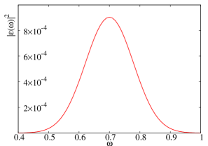
Figure 1: (color online). This plot shows the modulus square of the Fourier-transformed field of strength of $\epsilon_{1}=0.0067$au, which includes the first several excitation energies.

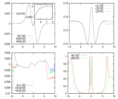
Figure 2: (color online). Densities and correlation potentials at time $t=22.440$au. The top-left shows the scaled density response $\delta n_{\alpha}(x,t)/\alpha$ for the three values of $\alpha$ indicated. The inset zooms in on the scaled density response in the outer region. The top-right shows the correlation potentials at different field strengths. The bottom-left panel plots the scaled correlation potential response, $\delta v_{c,\alpha}(x,t)/\alpha$. The steps of the correlation potentials occur where the density response is non-linear. The lower right panel plots the deviation from linearity, $M_{\alpha}$, of Eq. 5.

We choose a weak field strength $\epsilon_{1}=0.0067$au such that the predominant response of the system is linear. We then apply weaker fields, $\epsilon_{\alpha}$, of strengths: $\epsilon_{0.50}=\frac{\epsilon_{1}}{2}$ and $\epsilon_{0.25}=\frac{\epsilon_{1}}{4}$.

The top left panel of Figure 2 shows that the density response, defined as $\delta n_{\alpha}(x,t)=n_{\alpha}(x,t)-n(x,0)$, predominantly scales linearly with the field strength: plots of $\delta n_{\alpha}/\alpha$ lie essentially on top of each other. The correlation potential response, in the lower left panel, in region $\approx(-5,5)$ also scales linearly with the applied field but deviates from linearity outside this region, displaying step and peak structures; these are also evident in the full correlation potential plotted in the top right panel. Zooming into the tail regions of the densities (see e.g. inset of top panel), we see in fact the density response is not linear in these regions. The steps and peaks in the non-linear region do not scale with the field strength; we do not expect them to, as the response is not linear, and they also do not have any higher-order consistent scaling behavior with the field strength.

We have checked that the step features are not numerical artifacts: they are converged with respect to the size of the box and grid-spacing. Changing these parameters may change the details of the noise in the small oscillations visible in $\delta v_{\scriptscriptstyle\rm C}$ (much smaller scale than the scale of the step itself) but do not change the overall structure. This is true for all the graphs shown in the paper.

To quantify the deviation from linearity we next define a measure, which we plot in the lower right panel. Since the weakest strength is closest to the ideal linear response limit, we define the deviation relative to this strength, and define:

$$M_{\alpha}=\frac{|\delta n_{\alpha}-4\alpha\delta n_{0.25}|}{|\delta n_{\alpha}|+4\alpha|\delta n_{0.25}|}.$$ (5)

If the density response at field strength $\alpha$ was truly linear, the numerator would vanish (within the approximation that when $\alpha=0.25$ the system response is linear); and it is trivially zero when $\alpha=0.25$. The measure takes values from 0 to 1, growing as the degree of non-linearity grows. Note that when the signs of $\delta n_{\alpha}$ and $\delta n_{0.25}$ are opposite, the measure takes the value of 1. In the lower right panel in Figure  2, we see that, aside from a sharp peak structure near $x=0$, $M_{\alpha}$ is small in the region $x\approx(-5,5)$, then grows outside this region, peaking and remaining large after the peak. The sharp structure near $x=0$ occurs due to the density responses themselves going through zero near the origin. The step structures in the correlation potential appear only in the outer region, where the measure is appreciable, i.e. the density response is significantly non-linear.

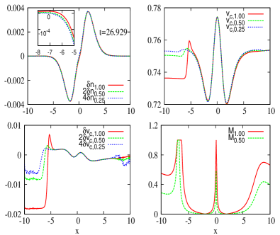
Figure 3: (color online). Densities and correlation potentials at time $t=26.929$au. See caption of Fig. 2 for details.

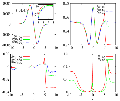
Figure 4: (color online). Densities and correlation potentials at time $t=31.417$au. See caption of Fig. 4 for details.

Figures 3 and 4 show the density responses and correlation potentials plotted in the same way, at two different times, $t=26.929$au and $t=31.417$au. The same conclusions can be drawn as for the earlier time, and in fact for all the different times throughout the time propagation that we analyzed: step structures appear only in regions where the system’s response is nonlinear. We did not find a single time at which steps occurred in a region where the density response is linear. The step structures do not scale in any consistent way with the field strength. (Where the system response is linear, the correlation potential response scales linearly with the field, as expected). There are times at which the step is abnormally large: this tends to happen in close-to-nodal structures of the density, and is likely a feature only of two-electron systems.

We note that regions of non-linear system response are typical in linear response calculations: essentially, the term representing the field in Hamiltonian $H_{0}+{\cal E}(t)x$ gets larger than the field-free term for large $x$, so a perturbative treatment of it in that region is no longer valid. However, such a calculation is still considered to be in the linear response regime, since these regions contribute negligibly to practical observables extracted from the system dynamics.

II.2 Dynamics under a “delta-kick”

A common way to obtain linear response spectra from real-time dynamics is to apply a “delta-kick” to the system at the initial time, and measure the subsequent free evolution YNIB96 . That is, ${\cal E}(t)=k\delta(t)$, so that we can write $\Psi(t=0^{+})=e^{ik\hat{x}}\Psi(t=0)$. For small enough kick strengths $k$, the system response is linear in $k$. Fourier transforming the time-dependent dipole moment yields the spectrum shown in Fig 5, where a value of $k=0.01$ was used. The peaks correspond to the singlet excited states of odd parity as these are dipole-allowed. The peak-frequencies shown can be confidently assigned to these states only up to about $\omega\sim 0.73$au, because the excited states of energies higher than this have spatial extent too large for the size of the box in our calculation (we have checked convergence with respect to box size for the lower excitations).

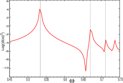
Figure 5: (color online). The dipole power spectrum obtained from solving the time-dependent Schrödinger equation. Vertical dashed lines indicate the dipole-allowed singlet transition energies, which agree with the energy spectrum. (Note the relative oscillator strengths are not accurate because the propagation time was not long enough.)

Now we consider the same analysis as in the previous case: we halve $k$ and study the response of the correlation potential and density, looking for the step feature. The main difference from the Gaussian pulse field is that now all the dipole-allowed singlet excited states are equally stimulated: the power spectrum for the delta-kick is uniform.

Figures 6 and 7 show the response densities and correlation potentials at two snapshots of time 400au and 1400au, respectively. Similar graphs appear at the other times we looked at. We again see steps and (sometimes large and oscillatory) peak-like structures, but, again, they appear only in the region of non-linear density-response; regions that contribute negligibly to the linear response observables. Once again, these structures are fully non-linear, in that there is no consistent scaling of their size with the field strength.

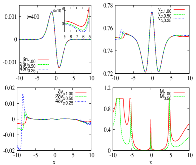
Figure 6: (color online). At time $400$au after the kick is applied, the response densities and correlation potentials are shown; please refer to Fig.1 for the details of the panels.

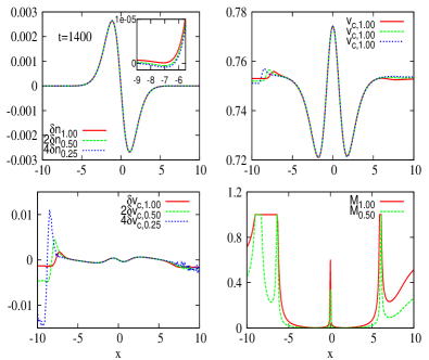
Figure 7: (color online). As in Figure 6 but for time 1400 au.

III Linear terms in $v_{\scriptscriptstyle\rm C}$ in field-free evolution of a perturbed ground-state

The dynamical step that was found in typical non-linear dynamics situations arises from the the fourth term of Eq. 2, as discussed in Ref. EFRM12 . Here we analyse that term, as well as the full correlation potential, in a linear response situation, by explicitly finding the terms that scale linearly with the deviation from the ground-state.

We consider field-free evolution of a perturbed ground state, for example, as would occur in the delta-kicked propagation of the previous section. We can then expand the wavefunction at time $t$ in terms of the eigenstates, $\Psi_{m}$, of the unperturbed system, as

$$\Psi(t)=e^{-iE_{0}t}\left(\Psi_{0}+\sum_{m}c_{m}e^{-i\omega_{m}t}\Psi_{m}\right)$$ (6)

where $\Psi_{0}$ is the ground-state, $\omega_{m}=E_{m}-E_{0}$ are excitation frequencies, and $c_{m}$ are expansion coefficients, to be considered the small parameter. For example, in the delta-kick of the previous section, $c_{m}=ik\langle\Psi_{0}|\hat{x}|\Psi_{m}\rangle$ (where, for the two electron case $\hat{x}=x_{1}+x_{2}$). (Note that in the general case, $c_{0}$ need not be zero). Then we may write, to first order in the $c_{m}$,

$$n(x,t)=n_{0}(x)-2i\sum_{m}c_{m}\sin(\omega_{m}t)n_{0m}(x)$$ (7)

where $n_{0}(x)$ is the ground-state density and $n_{0m}(x)=2\int dx^{\prime}\Psi_{0}(x,x^{\prime})\Psi_{m}(x,x^{\prime})$ is the $m$th transition density. Also, we have, to linear order in $c_{m}$,

$$j(x,t)=i\sum_{m}c_{m}\cos(\omega_{m}t)j_{0m},$$ (8)

where $j_{0m}(x)=2\int dx^{\prime}\left[\Psi_{m}{\partial}\Psi_{0}/{\partial}x-\Psi_{0}{\partial}\Psi_{m}/{\partial}x\right]$. So, to linear order in the $c_{m}$,

$$\int^{x}\partial_{t}u(x^{\prime},t)dx^{\prime}=-i\sum_{m\neq 0}c_{m}\omega_{m}\sin(\omega_{m}t)\int^{x}\frac{j_{0m}(x^{\prime})}{n_{0}(x^{\prime})}dx^{\prime}.$$ (9)

If there is any step in the correlation potential that appears at linear order, it must appear in this term. From computing just the excited state wavefunctions and their energies, the right hand side can easily be computed. Further, expanding all terms in Eq. (2) to linear order, and using Eq. (3), we get the response of the correlation potential to first order as:

$$\delta v_{\scriptscriptstyle\rm C}=\sum_{m\neq 0}ic_{m}\sin(\omega_{m}t)\left(\frac{({\partial}_{x}n_{0})^{2}}{2n_{0}^{2}}\left(\frac{{\partial}_{x}n_{0m}}{{\partial}_{x}n_{0}}-\frac{n_{0m}}{n_{0}}\right)-\frac{{\partial}_{x}^{2}n_{0}}{2n_{0}}\left(\frac{{\partial}_{x}^{2}n_{0m}}{{\partial}_{x}^{2}n_{0}}-\frac{n_{0m}}{n_{0}}\right)+\omega_{m}\int^{x}\frac{j_{0m}(x^{\prime})}{n_{0}(x^{\prime})}dx^{\prime}+\int\frac{n_{0m}(x^{\prime})}{\sqrt{(x-x^{\prime})^{2}+1}}dx^{\prime}\right).$$ (10)

(Note that the $c_{m}$ are pure imaginary, and the correlation potential is indeed purely real).

Plotting these terms for the delta-kicked soft-Coulomb well, where $c_{m}=2ikd_{0m}$, there is no step seen; as one moves out to larger x the terms can grow very large, but there is no step-structure. Figure 8 plots the response correlation potential arising from the lowest three dipole-accessible states (which are the first, third, and fifth excitations) in the sum of Eq. 10; the contributions from higher order terms decrease rapidly, due to the decreasing oscillator strength. Moreover, carrying out the expansion to second-order in $k$ there is also no evidence of step-like structure. This is consistent with results of previous section; the regions where there is a step are in fact where such an expansion does not hold, and the response of the system is fully non-linear.

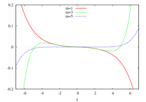
Figure 8: (color online). The correlation responses from first $3$ terms are plotted.

The results so far show that the dynamical step feature does not appear in linear response. That is, the lack of the non-adiabatic step feature in approximations does not affect the success of the approximations in predicting linear response, because this feature only appears in situations where the system response is non-linear. This conclusion has been based on the model 1D He atom, and we expect it to go through for the general three-dimensional $N$-electron case. A question might arise about systems that have states of multiple-excitation character in their linear response spectra: it is known that for TDDFT to capture such states the exchange-correlation kernel must have a frequency-dependence MZCB04 , indicating the underlying linear response exchange-correlation potential has an essentially non-adiabatic character. For the He atom (1D or 3D), such states however lie in the continuum and, although they can be accessed by the delta-kick perturbation TK09 , they contribute much less to the spectrum than the bound states and are outside the range of frequencies for which our dynamical simulations can be trusted. A better model to explore states of multiple-excitation character is a 1D model of a quantum dot: the Hooke’s atom, where two soft-coulomb interacting fermions live in a harmonic potential. The lowest singlet excitation is predominantly a single-excitation (excitation of the electronic center of mass coordinate), but the 2nd and 3rd excitations are (largely) mixtures of one single-excitation and one double-excitation EM11 ; MZCB04 ; one is the second excitation of the center of mass coordinate while the other is an excitation in the electronic relative coordinate. A dipole pertubation applied to such a system can only couple to the lowest excitation in linear response, a result that can be interpreted in terms of the harmonic potential theorem D94 . A quadratic kick however does excite the 2nd and 3rd excitations, and this is what we will consider now: we take

$$V(x,t)=\sum_{i=1}^{2}\frac{1}{2}\left(1+k\delta(t)\right)x_{i}^{2}$$ (11)

so that in Eq.6, $c_{m}=ik\langle\Psi_{0}|{\hat{x}}^{2}|\Psi_{m}\rangle$.

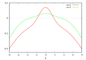
Figure 9: (color online). The correlation potential responses from double excitation contributions are plotted.

In Figure 9, we plot the contribution to the first-order correlation potential of Eq.10 of the two states of double-excitation character mentioned above. Once again, there is no step structure evident. The non-adiabaticity required to capture states of double-excitation in linear response is unrelated to the dynamical step feature uncovered in Ref. EFRM12 .

IV Summary

In this work, we studied the correlation potential of model two-electron systems in the linear response regime to investigate the role of the dynamical step feature found in recent studies of time-dynamics EFRM12 ; FERM13 . We applied a weak field to the soft-Coulomb helium atom for which we could extract the exact correlation potential. We found that step features in $v_{\scriptscriptstyle\rm C}$ only appear in regions far from the system, in the tails of the density, where the response of the system is in fact non-linear. These regions, by definition, do not contribute to the measured linear response of observables. These results therefore explicitly justify the expectation expressed in Ref. EFRM12 , that the non-adiabatic non-local step feature that was generically found there in the time-dependent correlation potential is a feature of non-linear dynamics, and is related to having appreciable population in excited states.

This explains why adiabatic approximations can usefully predict linear response spectra in general, while these same approximations may give incorrect time-dynamics in the non-perturbative regime EFRM12 ; FERM13 ; FHTR11 ; RG12 . The incorrect dynamics observed in the non-linear regime was due in part to the non-adiabatic non-local dynamical step found recently in these works, while the results here show that these are absent in the linear response regime. States of multiple-excitation character require a non-adiabatic approximation, but our analysis of the Hooke’s quantum dot model here has shown that this is unrelated to the appearance of the dynamical step: even in dynamics where double-excitations appear, the step still is absent in the linear response region.

Acknowledgments Financial support from the National Science Foundation CHE-1152784 (for K.L.), Department of Energy, Office of Basic Energy Sciences, Division of Chemical Sciences, Geosciences and Biosciences under Award DE-SC0008623 (N.T.M.), the European Communities FP7 through the CRONOS project Grant No. 280879 (PE), and a grant of computer time from the CUNY High Performance Computing Center under NSF Grants CNS-0855217 and CNS-0958379, are gratefully acknowledged.

References

- (1) P. Elliott, J. I. Fuks, A. Rubio, and N. T. Maitra, Phys. Rev. Lett. 109, 266404 (2012).
- (2) E. Runge and E.K.U. Gross, Phys. Rev. Lett. 52, 997 (1984).
- (3) Fundamentals of Time-Dependent Density Functional Theory, (Lecture Notes in Physics 837), eds. M.A.L. Marques, N.T. Maitra, F. Nogueira, E.K.U. Gross, and A. Rubio, (Springer-Verlag, Berlin, Heidelberg, 2012); and references therein.
- (4) Time-Dependent Density-Functional Theory: Concepts and Applications, C. A. Ullrich, (Oxford, 2012).
- (5) M. E. Casida and M. Huix-Rotllant, Annu. Rev. Phys. Chem. 63, 287, (2012).
- (6) J. D. Ramsden and R. W. Godby, Phys. Rev. Lett. 109, 036402 (2012).
- (7) J. I. Fuks, P. Elliott, A. Rubio, and N. T. Maitra, J. Phys. Chem. Lett. 4, 735 (2013).
- (8) N. T. Maitra, F. Zhang, R. Cave, K. Burke, J. Chem. Phys. 120, 5932 (2004).
- (9) D. Tozer and N. Handy, Phys. Chem. Chem. Phys. 2, 2117 (2000); M. E. Casida, J. Chem. Phys. 122, 054111 (2005); P. Romaniello et al, J. Chem. Phys. 130 044108 (2009); O. Gritsenko and E. J. Baerends, Phys. Chem. Chem. Phys. 11, 4640 (2009); M. Huix-Rotllant and M. E. Casida, http://arxiv.org/abs/1008.1478 (2010).
- (10) J. Javanainen, J.H. Eberly, Q. Su, Phys. Rev. A. 38, 3430 (1988).
- (11) D.M. Villeneuve, M.Yu. Ivanov, P.B. Corkum, Phys.Rev. A. 54, 736, (1996).
- (12) A.D. Bandrauk, N.H. Shon, Phys. Rev. A. 66, 031401, (2002).
- (13) T. Kreibich, M. Lein, V. Engel, E. K.U. Gross, Phys. Rev. Lett. 87, 103901 (2001).
- (14) D. G. Lappas and R. van Leeuwen, J. Phys. B: At. Mol. Opt. Phys. 31, L249 (1998).
- (15) F. Wilken and D. Bauer, Phys Rev Lett. 97, 203001 (2006).
- (16) M. Thiele, E.K.U. Gross, and S. Kümmel, Phys. Rev. Lett. 100, 153004 (2008).
- (17) M. Thiele and S. Kümmel, Phys. Chem. Chem. Phys. 11, 4630 (2009).
- (18) D. G. Tempel, N. T. Maitra, T. J. Martinez, J. Chem. Theory Comput. 5, 770 (2009).
- (19) J. I. Fuks, N. Helbig, I. V. Tokatly, A. Rubio, Phys. Rev. B. 84, 075107 (2011).
- (20) P. Elliott and N. T. Maitra, J. Chem. Phys. 135, 104110 (2011).
- (21) John F. Dobson, Phys. Rev. Lett. 73, 2244-7 (1994)
- (22) P. Hessler, N.T. Maitra, and K. Burke, J. Chem. Phys. 117, 72 (2002).
- (23) A. Castro et al., Phys. Stat. Sol. (b) 243, 2465 (2006).
- (24) M. A. L. Marques, A. Castro, G. F. Bertsch, and A. Rubio, Comp. Phys. Comm. 151, 60 (2003).
- (25) K. Yabana, T. Nakatsukasa, J.-I. Iwata and G. F. Bertsch, Phys. Stat. Sol. (b) 243, No. 5, 1121-1138 (2006)