Beam asymmetry $\Sigma$ for $\pi^{+}$ and $\pi^{0}$ photoproduction on the proton for photon energies from 1.102 to 1.862 GeV

Abstract

Beam asymmetries for the reactions $\gamma p\rightarrow p\pi^{0}$ and $\gamma p\rightarrow n\pi^{+}$ have been measured with the CEBAF Large Acceptance Spectrometer (CLAS) and a tagged, linearly polarized photon beam with energies from 1.102 to 1.862 GeV. A Fourier moment technique for extracting beam asymmetries from experimental data is described. The results reported here possess greater precision and finer energy resolution than previous measurements. Our data for both pion reactions appear to favor the SAID and Bonn-Gatchina scattering analyses over the older Mainz MAID predictions. After incorporating the present set of beam asymmetries into the world database, exploratory fits made with the SAID analysis indicate that the largest changes from previous fits are for properties of the $\Delta(1700)3/2^{-}$ and $\Delta(1905)5/2^{+}$ states.

I Introduction

The properties of the resonances for the non-strange baryons have been determined almost entirely from the results of pion-nucleon scattering analyses PDG . Other reactions have mainly served to fix branching ratios and photo-couplings. With the refinement of multi-channel fits and the availability of high-precision photoproduction data for both single- and double-meson production, identifications of some new states have emerged mainly due to evidence from reactions not involving single-pion-nucleon initial or final states PDG . However, beyond elastic pion-nucleon scattering, single-pion photoproduction remains the most studied source of resonance information.

Much of the effort aimed at providing complete or nearly-complete information for meson-nucleon photoproduction reactions has been directed to measuring double-polarization observables. However, often overlooked is that the data coverage for several single-polarization observables, also vital in determining the properties of the nucleon resonance spectrum, still remains incomplete. More complete datasets for those single-polarization observables can also offer important constraints on analyses of the photoproduction reaction.

In this work, using linearly-polarized photons and an unpolarized target, we provide a large set of beam asymmetry $\Sigma$ measurements from 1.102 to 1.862 GeV in laboratory photon energy, corresponding to a center-of-mass energy $W$ range of 1.7 to 2.1 GeV. As will be seen, this dataset greatly constrains multipole analyses above the second-resonance region in part simply due to the size of the dataset provided: with these new $\Sigma$ asymmetry data from the CEBAF Large Acceptance Spectrometer (CLAS) at Jefferson Lab in Hall B, the number of measurements in the world database for the processes $\gamma p\to\pi^{0}p$ and $\gamma p\to\pi^{+}n$ between 1100 and 1900 MeV for $E_{\gamma}$ is more than doubled. We will show here that there are unexpectedly large deviations between these data and some of the most extensive multipole analyses covering the resonance region. We have included these $\Sigma$ data in a new partial wave analysis and will compare that analysis with competing predictions in this paper.

The paper is organized in the following manner: We give a brief background of the experimental conditions for this study in Sec. II. An overview of the methods used to extract the beam asymmetry results reported here is given in Sec. III through Sec. VII, and the uncertainty estimates for the $\Sigma$ data obtained are given in Sec. VIII. The resulting data are summarized and described in Sec. IX. They are then are compared to various predictions and a new analysis presented here in Sec. X, where we also compare multipoles obtained with and without including the present data set. Conclusions are presented in Sec. XI.

II The running period

The beam asymmetries for the $\gamma\ p\rightarrow n\ \pi^{+}$ and $\gamma\ p\rightarrow p\ \pi^{0}$ reactions described in this paper were part of a set of experiments running at the same time with the same experimental configuration (cryogenic hydrogen target, bremsstrahlung photon tagger tag , and CLAS CLAS ) called the “g8b” run period. The “g8a” and “g8b” run periods were the first Jefferson Lab experiments to use the coherent bremsstahlung technique to produce polarized photons.

During the g8b running period, a bremsstrahlung photon beam with enhanced linear polarization was incident on a 40-cm-long liquid hydrogen target placed 20 cm upstream from the center of CLAS. The enhancement of linear polarization was accomplished through the coherent bremsstrahlung process by having the CEBAF electron beam, with an energy of 4.55 GeV, incident on a 50-$\mu$m-thick diamond radiator. The photon polarization plane (defined as the plane containing the electric-field vector) and the coherent edge energy of the enhanced polarization photon spectrum were controlled by adjusting the orientation of the diamond radiator using a remotely-controlled goniometer. The degrees of photon beam polarization are estimated via a bremsstrahlung calculation using knowledge of the goniometer orientation and the degree of collimation CBSA . Data with an unpolarized photon beam also were taken periodically using a graphite radiator (“amorphous runs”). For all data runs, the CLAS magnetic field was set to 50% of its maximum nominal field, with positive particles bending outward away from the axis determined by the incident photon beam. The event trigger required the coincidence of a post-bremsstrahlung electron passing through the focal plane of the photon tagger and at least one charged particle detected in CLAS.

The g8b run period was divided into intervals with different coherent edge energies, nominally set to 1.3, 1.5, 1.7, 1.9, and 2.1 GeV. In addition to the differing coherent edge energies (all measured at the same electron beam energy of 4.55 GeV), the data were further grouped into runs where the polarization plane was parallel to the floor (denoted as PARA) or perpendicular to the floor (denoted as PERP) or where the beam was unpolarized (amorphous). For the entire 1.9 GeV data set, the polarization plane was flipped between PARA and PERP automatically (“auto-flip”). Some of the 1.7 GeV data set was taken with auto-flip while for some runs, the polarization plane of the 1.7 GeV data was manually controlled (“manual”). For the 1.3 and 1.5 GeV data sets, all data used were of the manual type. (The 2.1 GeV data set was not utilized in the analysis.)

III Particle identification; kinematic variables

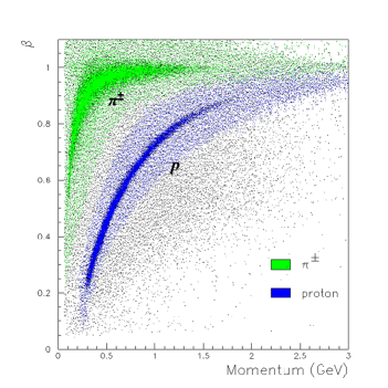
Figure 1: (Color online) Top panel: Velocity $\beta$ versus momentum $p$ for all charged particles passing through CLAS in this experiment. Bottom panel: Mass of charged particles passing through CLAS in this experiment as determined by $\beta$ and $p$. In each figure, pions and protons identified through the GPID algorithm are colored green and blue, respectively.

For experiments using the bremsstrahlung photon beam, the CLAS target region is surrounded by a scintillator array known as the “start counter”, which is used to establish the vertex time for the event startCounter . Particles then pass through drift chambers, which provide tracking information that yields momentum and angular information on charged particles passing through CLAS DC . Particles then pass through the time-of-flight scintillator array TOF , which, using the vertex time for the event, measures the time taken for the particle to pass from the start counter through the drift chambers. This time information determines the velocity of the charged particles passing through CLAS and, when coupled with the momentum information provided by the drift chambers, provides for determination of the mass and charge of the particle.

Figure 2: Top panel: Spectrum of squared missing mass $M_{X}^{2}$ from the reaction $\gamma\ p\rightarrow pX$. Bottom panel: Missing mass $M_{X}$ from the reaction $\gamma\ p\rightarrow\pi^{+}X$. The $\pi^{0}$, $\eta$, and neutron peaks are indicated on the plots.

Using the information obtained from the start counter, drift chambers, and TOF array for each particle scattered into CLAS, particle identification was performed with the GPID algorithm (described in gpid ). Plots showing $\beta$ versus $p$ and the mass distribution of the charged particles detected in CLAS, as determined by the GPID algorithm, are given in Fig. 1. As discussed in Ref. gpid , the GPID method uses the CLAS-measured momentum of the particle whose identity is to be determined, and calculates theoretical values of $\beta$ for the particle to be any one of all possible identities. Each one of the possible identities is tested by comparing the “theoretical” value of $\beta$ for a given particle type (using the reconstructed momentum information from CLAS) to the “measured” value of $\beta$ (as determined from time-of-flight information). The particle is assigned the identity that provides the closest expected value of $\beta$ to the empirically measured value of $\beta$. The identification for protons and pions is illustrated in Figure 1.

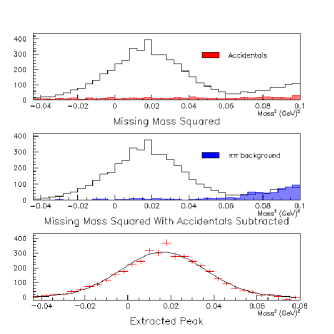
Figure 3: (Color online) Yield extraction examples from previously published g1c $\pi^{0}$ differential cross sections ASUpi0 . Shown are data for the $\pi^{0}$ yield extraction for $E_{\gamma}=1.425$ GeV and $\cos\theta^{p}_{\rm c.m.}$ = -0.45. The top panel is the missing mass yield for this bin, with the accidental contribution displayed in red. The accidental contribution is seen to be small and linear. The middle panel shows the missing mass distribution with the accidental contributions subtracted; the blue region indicates the 2-$\pi$ contribution determined. The bottom panel shows the extracted $\pi^{0}$ yield after contributions for accidentals and two-pion photoproduction have been subtracted from the missing mass distribution.

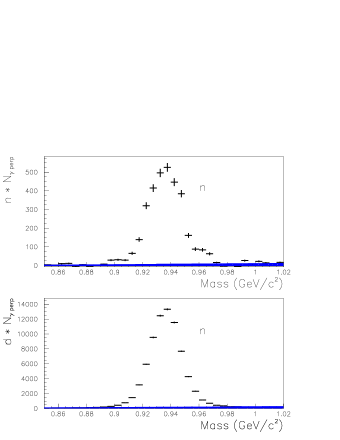
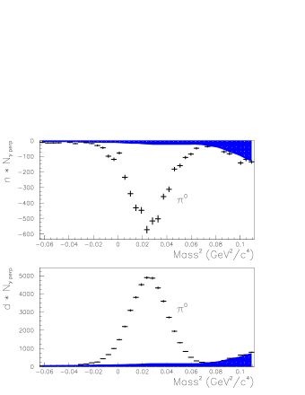
Figure 4: (Color online) Extraction of the quantities $n$ and $d$ (defined in Eqn. 20) for neutron (top two panels) and $\pi^{0}$ (bottom two panels) for the kinematic bin $\theta^{\pi}_{c.m.}=123^{\circ}$ and $E_{\gamma}=1229$ MeV. Top two panels: Reaction $\gamma p\rightarrow\pi^{+}n$. The $x$-axis is missing mass $M_{X}$ from the reaction $\gamma p\rightarrow\pi^{+}X$. Bottom two panels: Reaction $\gamma p\rightarrow p\pi^{0}$. The $x$-axis is squared missing mass $M_{X}^{2}$ from the reaction $\gamma p\rightarrow pX$. The blue shaded region in each plot represents contributions from background.

IV Missing mass reconstruction for $\mathbf{\pi}$ $\mathbf{N}$ final states

The kinematic quantities determined from the time-of-flight and drift chamber systems yield good momentum definition for the proton and $\pi^{+}$. The energy and momentum determined for each particle by CLAS were corrected for energy lost by that particle in passing through the material in both the target cell and the start counter in order to reconstruct the momentum at the vertex where the photoproduction reaction occurred using the standard CLAS algorithm for those corrections, ELOSS eloss . In addition to the energy loss correction, a CLAS momentum correction was used. The CLAS momentum correction optimized the momentum determination through kinematic fitting.

The scattering angle and momentum information for each particle was used to construct a missing mass $M_{X}$ based on the assumption that the reaction observed was $\gamma\ p\rightarrow\pi^{+}X$ or $\gamma\ p\rightarrow pX$, where $X$ is the other body in the two-body final state using the relation

$$M_{X}\!\!=\!\! \sqrt{m^{2}_{\pi^{+}}\!\!+m^{2}_{p}+2E_{\gamma}m_{p}\!\!-2E_{\pi^{+}}\!\!\left(m_{p}\!\!+E_{\gamma}\right)\!\!+\!\!2E_{\gamma}p_{z\pi^{+}}}$$

for the $\gamma\ p\rightarrow\pi^{+}X$ reaction, and

$$M_{X}\!\!=\!\!\sqrt{2m^{2}_{p}+2E_{\gamma}m_{p}-2E_{p}\left(m_{p}+E_{\gamma}\right)+2E_{\gamma}p_{zp}}$$

when the reaction is $\gamma\ p\rightarrow pX$, where $M_{X}$ is the mass of the missing particle, $E_{\gamma}$ is the incident photon energy, $m$ denotes mass, $p$ is the momentum, $p_{z}$ denotes the $z$-component of the momentum, and subscripts define the particle type.

Based on these assumptions, the missing mass spectrum for data in the full spectrometer acceptance for all photon energies within the 1.3 GeV coherent edge setting is shown in Fig. 2. The neutron and $\pi^{0}$ peaks are clearly seen.

V Fourier moment technique for extracting beam asymmetry $\Sigma$

Figure 5: Rough $\pi^{0}$ normalized yields for forward center-of-mass angles. Top panel shows the normalized yields for runs with the PERP polarization orientation, while the bottom shows the normalized yields for runs with the PARA orientation.

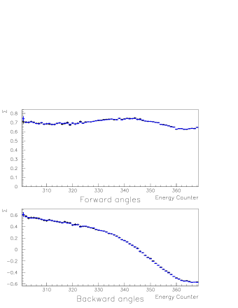
Figure 6: (Color online) Rough $\pi^{0}$ beam asymmetries $\Sigma$ for forward (top panel), and backward (bottom panel) center-of-mass angles determined for polarized photons associated with the indicated photon tagger energy counter. Blue points represent values of $\Sigma$ determined by the Fourier moment method, while black points represent values of $\Sigma$ determined by the $\phi$-bin method averaged over polarization orientations.

Traditionally, beam asymmetries have been extracted by breaking the azimuthal acceptance of the spectrometer into a very large number of bins, extracting the meson yields for those bins, and then fitting that distribution of yields with a linear-plus-cosine expression to determine $\Sigma$. As a more efficient procedure, the beam asymmetries for this experiment were extracted using a Fourier moment analysis of the polar and azimuthal scattering angle distributions of the particles detected in CLAS. An overview of the technique used to extract the beam asymmetries is presented here.

V.1 Definition of observables

Meson photoproduction differential cross sections may be written as

$$\frac{d^{2}{\sigma}}{d\Omega{dE}_{\gamma}},$$

where ${d}E_{\gamma}$ is the infinitesimal incident photon energy bin width and $d\Omega$ is the infinitesimal solid angle element in which the photoproduced meson is detected. (All quantities are center-of-mass quantities unless otherwise indicated.) Practically, however, the cross sections are measured in terms of finite kinematic bins in photon energy and scattering angle. Thus, what is measured is more accurately written

$$\Delta\sigma^{i,j,k}={\int_{E_{i-1}}^{E_{i}}}{\int_{\theta_{j-1}}^{\theta_{j}}}{\int_{\varphi_{k-1}}^{\varphi_{k}}}\frac{d^{2}{\sigma}}{d\cos(\theta){dE}_{\gamma}}{dE}_{\gamma}\sin(\theta)d\theta d\varphi,$$ (1)

where the indices $i,j,$ and $k$ denote the individual bin boundaries for incident photon energy $E_{\gamma}$, scattering polar angle $\theta$, and azimuthal scattering angle $\varphi$, respectively.

Experimentally, $\Delta\sigma^{i,j,k}$ in Eqn (1) is approximated by the relation

$$\Delta\sigma^{i,j,k}\approx\frac{Y^{i,j,k}}{N_{\gamma}^{i}\rho L\epsilon^{i,j,k}},$$ (2)

where $Y^{i,j,k}$ is the meson yield in kinematic bin $i,j,k$, $N_{\gamma}^{i}$ is the incident number of photons for bin $i$, $\rho$ is the target density, $L$ is the target length, and $\epsilon^{i,j,k}$ is the detector efficiency for kinematic bin $i,j,k$.

Figure 7: Frequency distribution for the rough $\pi^{0}$ data shown in Fig. 6 of the ratios of $\Sigma$ from the Fourier moment method divided by $\Sigma$ obtained from the $\phi$-bin method for each photon tagger energy counter. Top panel: Forward center-of-mass angles. Bottom panel: Backward center-of-mass angles. A Gaussian fit to each of these distributions is also shown.

As defined above, the photon beam polarization orientations used for the running period had either the electric field vector parallel to the Hall B floor (with the degree of polarization denoted by $P_{\|}$) or perpendicular to the floor (with the corresponding degree of polarization $P_{\bot}$). The differential cross sections for the various incident photon beam polarizations are labeled in the following fashion:

(a) for perpendicular beam polarization,

$$\frac{d{\sigma}_{\bot}}{d\Omega}=\frac{d{\sigma}_{a}}{d\Omega}[1+P_{\bot}\Sigma\cos(2\varphi)]$$ (3)

(b) for parallel beam polarization,

$$\frac{d{\sigma}_{\|}}{d\Omega}=\frac{d{\sigma}_{a}}{d\Omega}[1-P_{\|}\Sigma\cos(2\varphi)].$$ (4)

The unpolarized differential cross sections for a given reaction extracted from the amorphous carbon radiator is

$$\frac{d{\sigma}_{a}}{d\Omega}=\frac{1}{2}\left(\frac{d{\sigma}_{\bot}}{d\Omega}+\frac{d{\sigma}_{\|}}{d\Omega}\right).$$ (5)

V.2 Azimuthal moments for determining $\Sigma$

For this analysis, two additional $\varphi$-dependent quantities are defined:

$$f^{i,j}(\varphi)=\rho L{\int_{E_{i-1}}^{E_{i}}}{\int_{\theta_{j-1}}^{\theta_{j}}}\epsilon(E_{\gamma},\theta,\varphi)\frac{d^{2}{\sigma}}{d\Omega{dE}_{\gamma}}{dE}_{\gamma}\sin\theta d\theta$$

and

$$\tilde{Y}^{i,j}(\varphi)=\frac{Y^{i,j}(\varphi)}{N_{\gamma}^{i}},$$ (6)

where the former defines the normalized yield density with respect to azimuthal angle, and the latter is simply the normalized yield for a given $\varphi$ for bin $i,j$. These normalized yields may be further labeled by the photon beam polarization as $\tilde{Y}^{i,j}_{a}$, $\tilde{Y}^{i,j}_{\bot}$, and $\tilde{Y}^{i,j}_{\|}$, which would be the yield for the amorphous target, the yield with the perpendicularly polarized beam, and the yield with the parallel polarized beam, respectively.

Using the appropriate definitions given in Eqn (3), (4), and (5), the three normalized yields in Eqs. (6) may be written as

$$\tilde{Y}^{i,j}_{a}={\int_{0}^{2\pi}}f^{i,j}_{a}(\varphi)d\varphi$$ (7)

$$\tilde{Y}^{i,j}_{\bot}={\int_{0}^{2\pi}}f^{i,j}_{a}(\varphi)[1+P_{\bot}^{i}\Sigma^{i,j}\cos(2\varphi)]d\varphi$$ (8)

$$\tilde{Y}^{i,j}_{\|}={\int_{0}^{2\pi}}f^{i,j}_{a}(\varphi)[1-P_{\|}^{i}\Sigma^{i,j}\cos(2\varphi)]d\varphi.$$ (9)

With these definitions, all yields are now expressed in terms of various integrals involving the normalized yield density $f^{i,j}_{a}(\varphi)$, which is the normalized yield density for the amorphous carbon radiator. This function includes all physics effects modulated by the experimental acceptance $\epsilon^{i,j}$. The quantity $f^{i,j}_{a}(\varphi)$ is then expanded in a Fourier series as

$$f^{i,j}_{a}(\varphi)=a_{0}+\sum_{n=1}^{\infty}[a_{n}\cos(n\varphi)+b_{n}\sin(n\varphi)],$$ (10)

where each term of the series represents the $n^{\rm{th}}$ Fourier moment of $f^{i,j}_{a}$.

As usual, one can construct, event by event, a missing mass histogram for the reaction $\gamma p\rightarrow pX$ or $\gamma p\rightarrow\pi^{+}X$. In the approach used here, moment-$n$ histograms are constructed by taking each event in the $\gamma p\rightarrow pX$ or $\gamma p\rightarrow\pi^{+}X$ missing mass histogram and weighting each event by the value of $\cos(n\varphi)$ corresponding to that event for the various yields in (7)-(9).

Of particular importance are the moment-2 histograms

$$\tilde{Y}^{i,j}_{\bot 2} \equiv {\int_{0}^{2\pi}}f^{i,j}_{\bot}(\varphi)\cos(2\varphi)d\varphi$$ (11)

$$= {\int_{0}^{2\pi}}f^{i,j}_{a}(\varphi)\cos(2\varphi)d\varphi$$

$$+P_{\bot}\Sigma^{i,j}{\int_{0}^{2\pi}}f^{i,j}_{a}(\varphi)\cos^{2}(2\varphi)d\varphi$$

and

$$\tilde{Y}^{i,j}_{\|2} \equiv {\int_{0}^{2\pi}}f^{i,j}_{\|}(\varphi)\cos(2\varphi)d\varphi$$ (12)

$$= {\int_{0}^{2\pi}}f^{i,j}_{a}(\varphi)\cos(2\varphi)d\varphi$$

$$-P_{\|}\Sigma^{i,j}{\int_{0}^{2\pi}}f^{i,j}_{a}(\varphi)\cos^{2}(2\varphi)d\varphi.$$

Subtracting Eqn (12) from (11) yields

$$\tilde{Y}^{i,j}_{\Sigma} \equiv \tilde{Y}^{i,j}_{\bot 2}-\tilde{Y}^{i,j}_{\|2}$$

$$= (P_{\bot}^{i}+P_{\|}^{i})\Sigma^{i,j}{\int_{0}^{2\pi}}f^{i,j}_{a}(\varphi)\cos^{2}(2\varphi)d\varphi.$$

Using the double-angle relationship for the cosine of an angle, and keeping the Fourier series definition of $f^{i,j}_{a}(\varphi)$  from Eqn (10) in mind, this can be rewritten as

$$\tilde{Y}^{i,j}_{\Sigma} = \pi(P_{\bot}^{i}+P_{\|}^{i})\Sigma^{i,j}\left(a_{0}+\frac{a_{4}}{2}\right).$$ (14)

The polarization varies continuously during the course of a typical data run owing to fluctuations in the relative alignment of the incident electron beam and the diamond. Thus, the polarization must be determined continuously during a data run so that a photon-flux-weighted equivalent value of polarization for each run can be determined. The values of $P_{\|}$ and $P_{\bot}$ used in these equations are assumed to be these photon-flux-weighted values.

With these photon-flux-weighted equivalent values for the polarization $P_{\|}$ and $P_{\bot}$ and the histogram defined by Eqn (14), one only needs the Fourier coefficients $a_{0}$ and $a_{4}$ for $f^{i,j}_{a}(\varphi)$  to determine $\tilde{Y}^{i,j}_{\Sigma}$.

Figure 8: (Color online) Beam asymmetry $\Sigma$ for $\vec{\gamma}p\to\pi^{0}p$ at $E_{\gamma}=1102-1444$ MeV versus pion center-of-mass production angle. Photon energy is indicated by $E$, while the center-of-mass total energy is indicated by $W$. Solid (dash-dotted) lines correspond to the SAID DU13 (CM12 cm12 ) solution. Dashed (short-dashed) lines give the MAID07 Maid07 (BG2011-02 BnGa BnGa ) predictions. Experimental data are from the current (filled circles), Bonn CBELSA1 ; CBELSA2 (open circles), Yerevan Yerevan1 ; Yerevan2 ; Yerevan3 ; Yerevan4 ; Yerevan5 ; Yerevan6 (open triangle), GRAAL GRAAL1 (open square), CEA CEA (filled square), DNPL DNPL1 ; DNPL2 (cross), and LEPS LEPS (asterisk). Plotted uncertainties are statistical. The plotted points from previously published experimental data SAID are those data points within 3 MeV of the photon energy indicated on each panel.

Figure 9: (Color online) Beam asymmetry $\Sigma$ for $\vec{\gamma}p\to\pi^{0}p$ at $E_{\gamma}=1462-1862$ MeV versus pion center-of-mass production angle. The photon energy is shown as $E$. Notation as in Fig. 8.

Figure 10: (Color online) Beam asymmetry $\Sigma$ for $\vec{\gamma}p\to\pi^{+}n$ at $E_{\gamma}=1112-1862$ MeV versus pion center-of-mass production angle. The photon energy is shown as $E$. Solid (dash-dotted) lines correspond to the SAID DU13 (CM12 cm12 ) solution. Dashed (short-dashed) lines give the MAID07 Maid07 (BG2011-02 BnGa BnGa ) predictions. Experimental data are from the current (filled circles), GRAAL GRAAL2 (open square), Yerevan Yerevan7 (open triangle), CEA CEA (filled square), and DNPL DNPL2 (cross). Plotted uncertainties are statistical. The plotted points from previously published experimental data SAID are those data points within 3 MeV of the photon energy indicated on each panel.

Figure 11: (Color online) Fixed angle excitation functions of the beam asymmetry $\Sigma$ for $\vec{\gamma}p\to\pi^{0}p$. The pion center-of-mass production angle is shown. Notation as in Fig. 8.

Figure 12: (Color online) Fixed angle excitation functions of the beam asymmetry $\Sigma$ for $\vec{\gamma}p\to\pi^{+}n$. The pion center-of-mass production angle is shown. Notation as in Fig. 10.

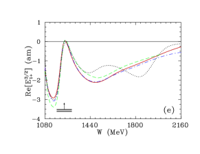
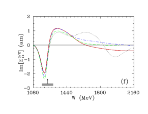
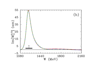
Figure 13: (Color online) Isospin $I$=3/2 multipole amplitudes from threshold to $W$ = 2.16 GeV ($E_{\gamma}$ = 2.02 GeV) for $l=0,1$. Solid (dash-dotted) lines correspond to the SAID DU13 (CM12 cm12 ) solution. Dashed (short-dashed) lines give MAID07 Maid07 , which terminates at $W$=2 GeV (BG2011-02 BnGa solution BnGa ). Vertical arrows indicate resonance energies $W_{R}$ and horizontal bars show full ($\Gamma$) and partial ($\Gamma_{\pi N}$) widths associated with the SAID $\pi N$ solution SP06 sp06 .

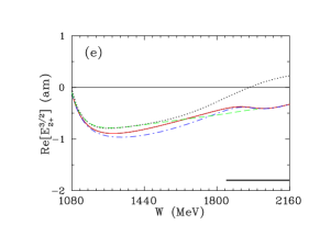
Figure 14: (Color online) Isospin $I$=3/2 multipole amplitudes from threshold to $W$ = 2.16 GeV ($E_{\gamma}$ = 2.02 GeV) for $l=2$. Notation as in Fig. 13.

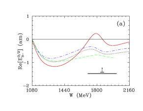
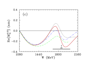
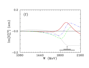
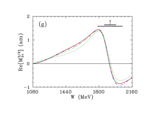
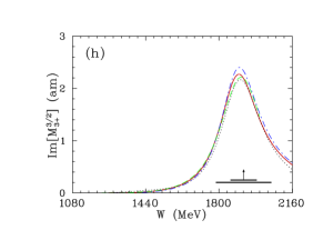
Figure 15: (Color online) Isospin $I$=3/2 multipole amplitudes from threshold to $W$ = 2.16 GeV ($E_{\gamma}$ = 2.02 GeV) for $l=3$. Notation as in Fig. 13.

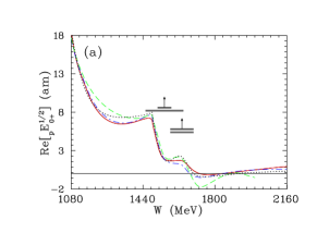
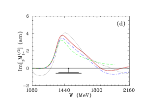
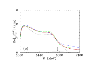
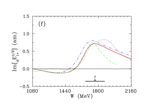
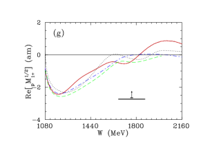
Figure 16: (Color online) Proton multipole $I$=1/2 amplitudes from threshold to $W$ = 2.16 GeV ($E_{\gamma}$ = 2.02 GeV) for $l=0,1$. Notation as in Fig. 13.

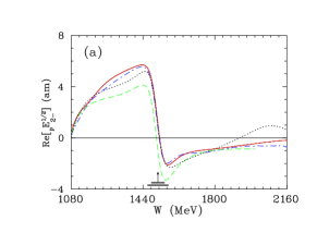
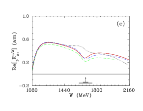
Figure 17: (Color online) Proton multipole $I$=1/2 amplitudes from threshold to $W$ = 2.16 GeV ($E_{\gamma}$ = 2.02 GeV) for $l=2$. Notation as in Fig. 13.

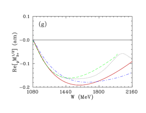
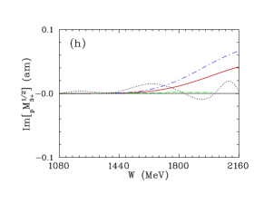
Figure 18: (Color online) Proton multipole $I$=1/2 amplitudes from threshold to $W$ = 2.16 GeV ($E_{\gamma}$ = 2.02 GeV) for $l=3$. Notation as in Fig. 13.

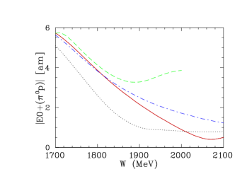
Figure 19: (Color online) Moduli of the $E_{0+}(\pi^{0}p)$ and $E_{0+}(\pi^{+}n)$ amplitudes. Notation is the same as in Fig. 13.

Obtaining the quantity $(a_{0}+\frac{a_{4}}{2})$ in Eqn (14) is straightforward using other moment-$n$ histograms. In a manner similar to that leading to Eqn (11) and (12), one obtains for the moment-0 histograms

$$\tilde{Y}^{i,j}_{\bot 0} = 2\pi a_{0}+P_{\bot}^{i}\Sigma^{i,j}\pi a_{2}$$

and

$$\tilde{Y}^{i,j}_{\|0} = 2\pi a_{0}-P_{\|}^{i}\Sigma^{i,j}\pi a_{2},$$

which gives

$$\tilde{Y}^{i,j}_{\bot 0}+\tilde{Y}^{i,j}_{\|0}\left(\frac{P_{\bot}^{i}}{P_{\|}^{i}}\right)=2\pi a_{0}\left(1+\frac{P_{\bot}^{i}}{P_{\|}^{i}}\right).$$ (15)

In a similar fashion, one obtains from the moment-4 histograms

$$\tilde{Y}^{i,j}_{\bot 4}+\tilde{Y}^{i,j}_{\|4}\left(\frac{P_{\bot}^{i}}{P_{\|}^{i}}\right)=\pi a_{4}\left(1+\frac{P_{\bot}^{i}}{P_{\|}^{i}}\right).$$ (16)

Finally, using the results of Eqs. (14), (15), and (16), one obtains

$$\tilde{Y}^{i,j}_{\Sigma}=\Sigma^{i,j}\left\{\frac{P_{\|}^{i}}{2}(\tilde{Y}^{i,j}_{\bot 0}+\tilde{Y}^{i,j}_{\bot 4})+\frac{P_{\bot}^{i}}{2}(\tilde{Y}^{i,j}_{\|0}+\tilde{Y}^{i,j}_{\|4})\right\}.$$ (17)

Combining Eqn (V.2) and (17), the beam asymmetry $\Sigma$ for kinematic bin $i$, $j$ is found to be

$$\Sigma^{i,j}=\frac{\tilde{Y}^{i,j}_{\bot 2}-\tilde{Y}^{i,j}_{\|2}}{\frac{P_{\|}^{i}}{2}(\tilde{Y}^{i,j}_{\bot 0}+\tilde{\ Y}^{i,j}_{\bot 4})+\frac{P_{\bot}^{i}}{2}(\tilde{Y}^{i,j}_{\|0}+\tilde{Y}^{i,j}_{\|4})}.$$ (18)

However, as it stands, the value of $\Sigma^{i,j}$ generated by the ratio in Eqn (18) is the beam asymmetry for whatever is in that particular kinematic bin, which will include not only the particular peak of interest but also any background within that particular kinematic bin. The interest here, instead, is the beam asymmetry associated with the photoproduction of a particular meson, which appears as a peak in the missing mass spectrum, and not the associated background beneath that peak. In practice, then, one extracts from the various histograms in the numerator and denominator in Eqn (18) the yield of the particular meson peak corresponding to the reaction of interest.

In order to simplify the notation below, the incident photon energy bin index $i$ and $\cos(\theta)$ bin index $j$ will be suppressed hereafter. The beam asymmetry is thus written as

$$\Sigma=\frac{\tilde{Y}_{\bot 2}-\tilde{Y}_{\|2}}{\frac{P_{\|}}{2}(\tilde{Y}_{\bot 0}+\tilde{Y}_{\bot 4})+\frac{P_{\bot}}{2}(\tilde{Y}_{\|0}+\tilde{Y}_{\|4})}.$$ (19)

Eqn (19) is the principal result for this method. With this approach, rather than partitioning the data for a given $E_{\gamma}$  and $\cos(\theta)$ into various $\varphi$ bins, all the data for a given $E_{\gamma}$   and $\cos(\theta)$ are used simultaneously to determine the beam asymmetry $\Sigma$ for the reaction of interest.

V.3 Statistical uncertainty

Because the various components of Eqn. (19) have non-vanishing covariances, the determination of statistical uncertainties, while straightforward, requires attention.

We begin by defining $w_{m,k,l}$ as the histogram weighting of the $l^{th}$ Poisson-distributed event, of the $m^{th}$ moment within the $k^{th}$ mass bin of a moment histogram $\tilde{Y}_{m}$. It then follows that the total occupancy $\tilde{Y}_{m,k}$ of the $k^{\rm{th}}$ bin within $\tilde{Y}_{m}$ is

$$\tilde{Y}_{m,k}=\frac{1}{N_{\gamma}}\sum_{l=1}^{Y_{0,k}}w_{m,k,l},$$

where $Y_{0,k}$ is the total number of events in bin $k$. For $m=0$ this is simply

$$\tilde{Y}_{0,k}=\frac{1}{N_{\gamma}}\sum_{l=1}^{Y_{0,k}}1=\frac{Y_{0,k}}{N_{\gamma}},$$

as expected. For all other moments

$$\tilde{Y}_{m,k}=\frac{1}{N_{\gamma}}\sum_{l=1}^{Y_{0,k}}\cos(m\varphi_{l}).$$

It now follows that the variance $\sigma^{2}_{\tilde{Y}_{m,k}}$ is given by

$$\sigma^{2}_{\tilde{Y}_{m,k}}=\frac{1}{(N_{\gamma})^{2}}\sum_{l=1}^{Y_{0,k}}\cos^{2}(m\varphi_{l}),$$

which for $m=0$, reduces to the familiar form for a Poisson distributed random variable divided by a constant term $N_{\gamma}$,

$$\sigma^{2}_{\tilde{Y}_{0,k}}=\frac{1}{(N_{\gamma})^{2}}\sum_{l=1}^{Y_{0,k}}1=\frac{1}{(N_{\gamma})^{2}}Y_{0,k}=\frac{1}{N_{\gamma}}\tilde{Y}_{0,k}.$$

It is useful to note that, by way of the double-angle relationship for the cosine of an angle, the variance of $\tilde{Y}_{m,k}$ can be written as

$$\sigma^{2}_{\tilde{Y}_{m,k}}=\frac{1}{2(N_{\gamma})^{2}}\sum_{l=1}^{Y_{0,k}}\left[1+\cos(2m\varphi_{l})\right]=\frac{1}{2N_{\gamma}}\left[\tilde{Y}_{0,k}+\tilde{Y}_{2m,k}\right].$$

The covariance of two variables $\tilde{Y}_{m1,k}$, and $\tilde{Y}_{m2,k}$, ${\rm{Cov}}(\tilde{Y}_{m_{1},k},\tilde{Y}_{m_{2},k})$, is given by

$${\rm{Cov}}(\tilde{Y}_{m_{1},k},\tilde{Y}_{m_{2},k}) = \frac{1}{(N_{\gamma})^{2}}\sum_{l=1}^{Y_{0,k}}\cos(m_{1}\varphi_{l})\cos(m_{2}\varphi_{l})$$

In what follows the identity

$${\rm{Cov}}(\tilde{Y}_{m,k},\tilde{Y}_{2m,k}) = \frac{1}{(N_{\gamma})^{2}}\sum_{l=1}^{Y_{0,k}}\cos(m\varphi_{l})\cos(2m\varphi_{l})$$

$$= \frac{1}{(N_{\gamma})^{2}}\sum_{l=1}^{Y_{0,k}}\frac{1}{2}(\cos(m\varphi_{l})+\cos(3m\varphi_{l}))$$

$$= \frac{1}{2(N_{\gamma})^{2}}(\tilde{Y}_{m,k}+\tilde{Y}_{3m,k})$$

will be of use, as well as

$${\rm{Cov}}(\tilde{Y}_{0,k},\tilde{Y}_{m,k}) = \frac{1}{N_{\gamma}}\tilde{Y}_{m,k}.$$

With these preliminaries, the statistical uncertainty for the beam asymmetry $\Sigma$ given by Eqn (19) can be determined.

By allowing the following definitions of the numerator and denominator of Eqn. (19),

$$n \equiv \tilde{Y}_{\bot 2}-\tilde{Y}_{\|2}$$

$$d \equiv \frac{P_{\|}^{i}}{2}(\tilde{Y}_{\bot 0}+\tilde{Y}_{\bot 4})+\frac{P_{\bot}^{i}}{2}(\tilde{Y}_{\|0}+\tilde{Y}_{\|4}),$$ (20)

we can then rewrite the beam asymmetry $\Sigma$ in the form

$$\Sigma=\frac{n}{d}.$$

The variance of $\Sigma$ is then

$$\sigma^{2}_{\Sigma}=\Sigma^{2}\left\{\frac{\sigma^{2}_{n}}{n^{2}}+\frac{\sigma^{2}_{d}}{d^{2}}-\frac{2{\rm{Cov}}(n,d)}{nd}.\right\}$$

We can now determine the variance of $n$, $d$, and the covariance of $n,d$. The variance of $n$ is

$$\sigma^{2}_{n} = \frac{1}{2N_{\gamma\bot}}(\tilde{Y}_{\bot 0}+\tilde{Y}_{\bot 4})+\frac{1}{2N_{\gamma\|}}(\tilde{Y}_{\|0}+\tilde{Y}_{\|4}),$$

where $N_{\gamma\bot}$ ($N_{\gamma\|}$) is the integrated photon flux for perpendicular (parallel) photon beam orientation. The variance of $d$ is

$$\sigma^{2}_{d} = \frac{P_{\|}^{2}}{4N_{\gamma\bot}}(\tilde{Y}_{\bot 0}+\frac{1}{2}(\tilde{Y}_{\bot 0}+\tilde{Y}_{\bot 8})+2\tilde{Y}_{\bot 4})$$

$$+ \frac{P_{\bot}^{2}}{4N_{\gamma\|}}(\tilde{Y}_{\|0}+\frac{1}{2}(\tilde{Y}_{\|0}+\tilde{Y}_{\|8})+2\tilde{Y}_{\|4})$$

and the covariance of $n$, $d$

$${\rm{Cov}}(n,d) = \frac{P_{\|}}{4N_{\gamma\bot}}(3\tilde{Y}_{\bot 2}+\tilde{Y}_{\bot 6})-\frac{P_{\bot}}{4N_{\gamma\|}}(3\tilde{Y}_{\|2}+\tilde{Y}_{\|6}).$$

All the necessary quantities needed to calculate $\Sigma$ and the associated uncertainty $\sigma_{\Sigma}$ have now been derived.

VI Yield determination for each kinematic bin

To determine the $\pi^{0}$ yields, a technique very similar to the one used for the g1c experiment of extracted differential cross sections for $\pi^{0}$ photoproduction off the proton ASUpi0 was employed. The g1c experiment utilized the same CLAS detector and bremsstrahlung photon tagger as the g8b experiment, but had an 18-cm-long liquid hydrogen target placed at the center of CLAS, and only used unpolarized incident photons.

Following the previous discussion, the beam asymmetries were determined for a particular photon energy and $\cos(\theta)$ bin, which we call a “kinematic bin”. For each missing mass spectrum within each kinematic bin, the $\pi^{0}$ yield was extracted by removing the background under the peak. It was assumed that the background in the missing mass spectra arises from two particular types of events:

• Events arising from accidental coincidences between CLAS and the photon tagger.

• Events arising from two-pion photoproduction via the reaction $\gamma p\rightarrow p\pi^{+}\pi^{-}$.

The spectrum for accidental coincidences can be determined by looking at events that fell outside the designated trigger window. From experience with the g1c experiment, the background coming from accidentals within the g8b data set was approximated as being linear in missing mass. Figure 3 shows an example of the background subtraction from the CLAS published g1c pion differential cross sections ASUpi0 , where the accidental contribution was determined by looking at events that fell outside the designated trigger window. As can be seen in Fig. 3 the assumption that the accidentals are well modeled by a linear function is reasonable.

To determine the two-pion background, data for the reaction $\gamma\ p\rightarrow p\ \pi^{+}\ \pi^{-}$ were selected by requiring that each particle in the final state had to be identified through normal particle ID procedures, that the same incident photon was chosen for each particle, and that the missing mass was consistent with zero; the criterion for consistency with zero mass was if the mass $m_{Y}^{2}$, in the reaction $\gamma\ p\rightarrow p\ \pi^{+}\ \pi^{-}\ Y$ was less than 0.005 GeV² and greater than -0.01 GeV. These selected data were used to determine the shape of the $\pi^{+}\pi^{-}$ component of the background for the $\gamma p\rightarrow p\pi^{0}$ reaction in each kinematic bin.

The background subtraction for the $\pi^{0}$ was then performed in the following manner:

• The spectrum of missing mass $M_{X}$ in the $\gamma p\to pX$ reaction was fit with a functional form that included the linear approximation of the accidentals and the shape determined for the charged background noted above. A total of 3 parameters were varied: two parameters for the accidental contribution (modelled by a linear function) and one parameter for the magnitude of the charged background.

• The backgrounds determined in the previous step were subtracted from the yield.

• The background subtracted yield was then fit with a Gaussian and the standard deviation and centroid of the peak were determined.

• The region of the histogram resulting from step 3 that was within three times the standard deviation of the peak centroid was then determined to be the $\gamma p\to p\pi^{0}$ yield in the extracted $\pi^{0}$ peak.

For the extraction of the yield of the neutron peak from the reaction $\gamma p\rightarrow\pi^{+}X$, it was found that the 2$\pi$ background was negligible, and the only significant background was from accidentals. For this reason, only a linear approximation of the accidentals was included in the background determination for the neutron.

An example of the background subtraction for both neutron and $\pi^{0}$ extraction can be seen in Fig. 4.

VII Relative Normalization

For the measurement of beam asymmetry, knowledge of the absolute number of incident photons is not required. Instead, only the relative photon normalization between PARA and PERP running conditions is necessary. In order to obtain the relative photon normalization of PARA to PERP, a “rough $\pi^{0}$” measurement was used, where “rough $\pi^{0}$” is defined as any event detected from $\gamma\ p\rightarrow pX$ with missing mass $M_{X}$ between 0.0 and 0.25 GeV and, in this instance, $0\leq\cos(\theta^{X}_{c.m.})\leq 1$, where $\cos(\theta^{X}_{c.m.})$ is the meson center-of-mass scattering angle.

For the determination of the relative normalization, the more conventional approach of binning the rough $\pi^{0}$ data into azimuthal angle bins was used. The data were binned in the same $E_{\gamma}$ bins as for the moment extraction method, and in addition, the data were binned further into 36 azimuthal bins.

Once the yield for $\pi^{0}$ mesons was determined for each the running conditions, two quantities for each {$E_{\gamma}$, $\varphi$} bin were formed,

$$g_{\bot}\equiv\frac{Y_{\bot}}{Y_{a}}$$

and

$$g_{\|}\equiv\frac{Y_{\|}}{Y_{a}}.$$

These were fit to

$$g_{\bot}=A_{\bot}[1+B\cos(2\varphi)]$$

and

$$g_{\|}=A_{\|}[1-B\cos(2\varphi)],$$

where $A_{\|}={N_{\bot}}/{N_{a}}$, $A_{\bot}={N_{\|}}/{N_{a}}$, $B=P\Sigma$, and $N_{\bot}$, $N_{\|}$, $N_{a}$ represent the number of incident photons for the PERP, PARA, and amorphous running conditions respectively.

The values of $A$ taken from the parallel polarized beam orientation were divided by the values derived from the perpendicular orientation. The fractional values of $A_{\|}/A_{\bot}$ were found for each energy to determine the value of $N_{\|\gamma}/N_{\bot\gamma}$ from the relation $A_{\|}/A_{\bot}=N_{\|\gamma}/N_{\bot\gamma}$.

VIII Uncertainties

The statistical uncertainties for $\Sigma$ were obtained using the expressions given in subsection V.3. Systematic uncertainties for $\Sigma$ are dominated by the systematics of the polarization and relative normalization since many of the experimental quantities cancel in the ratio $\Sigma$.

The relative normalization was primarily dependent upon the total number of $\gamma p\rightarrow pX$ events having a missing mass (mass $X$) between 0 and 0.25 GeV. The statistics for such events were quite good and we take the systematic uncertainty of the relative normalization as being negligible.

One possible systematic error could come from imperfect knowledge of the orientation of beam polarization. To study the orientation of the beam polarization we took rough $\pi^{0}$ measurements for each orientation of the beam polarization (PERP and PARA) and normalized each type by the rough $\pi^{0}$ results from the amorphous runs. Using the entire set of runs from the 1.3 GeV coherent edge setting, the resulting rough $\pi^{0}$ normalized yields were placed in 90 $\varphi$-bins, and 50 MeV wide photon energy bins. The resulting $\varphi$-distributions were then fit to the function $A(1+B\cos(2\varphi+2C))$, with $A$, $B$, and $C$ being fit parameters. From the fit we were able to extract the possible azimuthal offset by reading out parameter $C$. Figure 5 shows the resulting fit for both orientations at photon energy of 1275 MeV. (The figure also clearly shows the six sector structure of CLAS.) We performed the fitting procedure for five energy bins from the 1.3 GeV data, took the weighted average, and obtained a possible systematic error in the polarization orientation of 0.07 $\pm$ 0.04 degrees. Since the possible systematic error is so small, we have assumed that such an error has a negligible effect on the beam asymmetry measurements.

The overall accuracy of the estimated photon polarization is difficult to determine. However, the consistency of the bremsstrahlung calculation could be checked by comparing predicted and measured polarization ratios for adjacent coherent edge settings in regions where overlapping energies exist. After consistency corrections were applied pCor , the estimated value for the photon polarization was self-consistent to within 4%. Therefore, the estimated systematic uncertainty in the photon polarization is taken to be 4%.

To test the dependence of the Fourier moment method on the polarization values, rough $\pi^{0}$ beam asymmetries from the moment method were compared to the beam asymmetries obtained using the $\varphi$-bin method (averaged over polarization orientations). As in Section VII, a rough $\pi^{0}$ azimuthal distribution was extracted for each tagger energy counter (E-counter). This time, however, the rough $\pi^{0}$ extraction was performed for the backward center-of-mass pion-angles ($-1\leq\cos(\theta^{X}_{c.m.})\leq 0$), as well as the forward center-of-mass pion-angles ($0\leq\cos(\theta^{X}_{c.m.})\leq 1$).

For each case (forward and backward angle events), the polarized photon data were divided by the corresponding distribution from amorphous data. As done in Sec. VII, the ratios for the azimuthal distributions were then fit to the expression

$$A\left[1+B\cos(2\varphi)\right],$$ (21)

where $A$ and $B$ were parameters of the fit. The value of beam asymmetry was then determined by $\Sigma=B_{\perp}/P_{\perp}$ ($\Sigma=-B_{||}/P_{||}$).

The values of $\Sigma$ determined from the $\varphi$-bin for each polarization orientation were averaged to obtain an average $\Sigma$ value. The average $\Sigma$ value obtained from the $\varphi$-bin method is compared to the beam asymmetries determined by the moment method, as seen in Figure 6. The top panel of Fig. 6 shows the rough $\pi^{0}$ beam asymmetries as a function of energy counter for the forward center-of-mass angles, and the backward center-of-mass angles are shown on the bottom panel. In each panel of Fig. 6 the black points are $\Sigma$ determined by the $\varphi$-bin method and the blue points represent $\Sigma$ determined from the moment method. A visual inspection of the plots given in Fig. 6 shows that the $\varphi$-bin and moment methods give very similar results.

To quantify the level of agreement between the two methods, the $\Sigma$ results from the moment method were divided by those of the $\varphi$-bin method on an E-counter by E-counter basis. A frequency plot of the resulting $\Sigma$-fractions ($\Sigma$ from moment method divided by $\Sigma$ from $\varphi$-bin method) was created for forward and backward center-of-mass angles of the $\pi^{0}$. In the top panel of Fig. 7 the frequency of $\Sigma$-fractions for forward angles is shown, while the bottom panel is the frequency plot for backward angles. A Gaussian was fit to each distribution of Fig. 7 with the results shown in Table 1.

Table 1: Gaussian parameters of the fit to the ratios of the results for $\Sigma$ using the moment method to $\Sigma$ determined by the $\varphi$-bin method on an E-counter by E-counter basis.

Center-of-mass angles	Center	$\sigma$
Forward	0.9978(3)	0.0043(4)
Backward	1.003(2)	0.015(2)

Since the beam asymmetry results from the moment method are well within 1% of the beam asymmetry results coming from the average value (parallel and perpendicular orientations) determined by the $\varphi$-bin method, we can safely say that the systematic uncertainty of the moment method due to polarization is nearly identical to the systematics one obtains when simply averaging the beam asymmetry from each polarization orientation. Thus, the fractional uncertainty of each polarization systematic uncertainty (each estimated as 4%) is added in quadrature to obtain an estimate of the systematic uncertainty in the beam asymmetry of 6%.

IX Results

The CLAS beam asymmetries obtained here for $\vec{\gamma}p\rightarrow p\pi^{0}$ (700 data points represented as filled circles) are compared in Figs. 8$-$9 with previous data from Bonn CBELSA1 ; CBELSA2 (open circles), Yerevan Yerevan1 ; Yerevan2 ; Yerevan3 ; Yerevan4 ; Yerevan5 ; Yerevan6 (open triangle), GRAAL GRAAL1 (open squares), CEA CEA (filled squares), DNPL DNPL1 ; DNPL2 (crosses), and LEPS LEPS (asterisks). The results for the reaction $\gamma p\rightarrow n\pi^{+}$ CLAS beam asymmetries (386 data points shown as filled circles) are compared in Fig. 10 to previous data from GRAAL GRAAL2 (open squares), Yerevan Yerevan7 (open triangles), CEA CEA (filled squares), and DNPL DNPL2 (crosses). Only those world data that are within $\pm$3 MeV of the CLAS photon energies $E_{\gamma}$ are shown. In addition to the data, phenomenological curves are included in the above mentioned figures and will be discussed further below.

For the CLAS $\pi^{0}$ data obtained here, the Yerevan results agree well except for a few points at $E_{\gamma}=$1265, 1301, and 1337 MeV. The Bonn data are comprised of two separate experiments CBELSA1 ; CBELSA2 , one published in 2009 CBELSA1 and another published in 2010 CBELSA2 . Typically, the CLAS results agree within error bars of the Bonn data, and where there is disagreement, it is almost always with the earlier 2009 results. The data obtained here is in very good agreement with DNPL at $E_{\gamma}=1337$ MeV and tend to be within error bars for all other energies except for $E_{\gamma}=1301$ MeV, where several DNPL points are systematically larger than the CLAS results. In particular, the data obtained here confirm the magnitude of the sharp structure seen in the DNPL data near $60^{\circ}$ for photon energies greater than about $E_{\gamma}=$ 1600 MeV. The LEPS results ($E_{\gamma}$ = 1551 MeV, backward angles), as well as the GRAAL results look systematically smaller when compared to CLAS.

The $\pi^{+}$ data obtained here tend to agree well with the previous data except for a few points. Out of the 34 points from GRAAL, easily identifiable differences between GRAAL GRAAL2 and CLAS occur for four with $E_{\gamma}=1148$ MeV ($\theta=114^{\circ}$, $122^{\circ}$, $145^{\circ}$, and $150^{\circ}$), along with a single point at $E_{\gamma}=1400$ ($\theta=90^{\circ}$). The single CEA CEA point at $E_{\gamma}=1400$ MeV ($\theta=90^{\circ}$) is systematicaly low when compared to CLAS. For the single Yerevan measurment of beam asymmetry Yerevan7 , the agreement is good. Comparisons between CLAS and DNPL DNPL2 are mixed. The DNPL results were taken with two different sets of beam energies. There was a low energy data set from DNPL with photon energies ranging from 520 to 1650 MeV, and a high energy data set with energies between 1650 and 2250 MeV. Because the DNPL energy ranges overlap for $E_{\gamma}=1650$ MeV, they report two sets of beam asymmetries for that energy. The DNPL data from the low energy data set agrees well with CLAS except for a single point at $E_{\gamma}=1400$ MeV ($\theta=75^{\circ}$), while the agreement between CLAS and the DNPL high energy data set is sometimes poor. In particular, at $E_{\gamma}=1649$ MeV, the DNPL points that are systematicaly high (low) compared to CLAS occuring at $\theta=$ 30^∘, 40^∘, 75^∘ ($\theta=$ 105^∘, 115^∘) are all from the DNPL high energy data set, while the agreement between CLAS and DNPL at $E_{\gamma}=1649$ MeV from the low energy data set is in good agreement.

Briefly, then, the new CLAS measurements generally are in agreement with older results within uncertainties, but the results presented here are far more precise and provide finer energy resolution.

X Comparison to Fits and Predictions

X.1 Comparison to phenomenological models

In Figs. 8$-$10, the $\Sigma$ data are shown along with predictions from previous SAID cm12 , MAID Maid07 (up to its stated applicability limit at a center-of-mass energy $W=$ 2 GeV, corresponding to $E_{\gamma}$ = 1.66 GeV), and the Bonn-Gatchina (BnGa, BnGa ) multipole analyses. Also shown are the results of an updated SAID fit (DU13) which includes the new data reported here. In order to increase the influence of these new precise data, the CLAS data reported here were weighted by an arbitrary factor of 4 in the fit. Figs. 11 and 12 show fixed angle excitation functions for $\vec{\gamma}p\to\pi^{0}p$ and $\vec{\gamma}p\to\pi^{+}n$.

For energies below that of the data presented in this paper, the neutral-pion production data are well represented by predictions from the multipole analyses up to a center-of-mass energy of about 1500 MeV. Above this energy, large differences are seen at very forward angles. The data appear to favor the SAID and BnGa predictions, with large differences between the SAID and BnGa values mainly at angles more forward than are reached in the present experiment. Pronounced dips seen in Figs. 8 and 9 for the reaction $\gamma p\to\pi^{0}p$, are qualitatively predicted by the three multipole analyses. These dips develop at angles slightly above 60^∘ and slightly below 120^∘ (note that these angles are related by the space reflection transformation $\theta\to\pi-\theta$). Our data confirm this feature suggested by earlier measurements, however those previous data were not precise enough to establish the sharpness of the dips. The revised SAID fit (DU13) now has these sharp structures. Below we shall discuss in more detail a possible source of the dip structure seen in the data.

For the charged-pion reaction, the MAID predictions are surprisingly far from the data over most of the measured energy range, and particularly at more backward angles. Over much of this range the SAID, BnGa, and revised SAID curves are nearly overlapping.

The fit $\chi^{2}$ per data point $\chi^{2}/N_{p}$ for DU13 is significantly improved over that from the CM12 SAID prediction  cm12 . The comparison given in Table 2 shows that, for the new DU13 fit, $\chi^{2}/N_{p}$ for the $\pi^{0}p$ channel is 2.77 and $\chi^{2}/N_{p}$ for the $\pi^{+}n$ channel is 2.77, an improvement by over an order of magnitude for that $\chi^{2}/N_{p}$ statistic when compared with the CM12 prediction. While the fit $\chi^{2}$ per datum is 2.77 when solely compared to the new CLAS data reported here, Table 2 also indicates that the fit to the previously published $\Sigma$ data is actually improved slightly in DU13 versus CM12, decreasing to 3.67 from 3.99. This is due to the added weighting of the $\Sigma$ data reported here in the fit, and also provides additional statistical confirmation of the consistency of the overall present and prior measurements, despite the differences noted above.

Table 2: Comparison of $\chi^{2}$ per data point for the beam asymmetry $\Sigma$ for the $\pi^{0}p$ and $\pi^{+}n$ channels using the predictions of the CM12 SAID solution  cm12 and the results of a fit (DU13) to the CLAS data reported here. Comparisons are provided for the CLAS data, previously published data, and for a dataset containing both the CLAS data (weighted by a factor of 4) and the previously published data. The number of data points used in each comparison is indicated by $N_{p}$.

Data	Solution	$\Sigma(\pi^{0}p)$	$\Sigma(\pi^{+}n)$
		$\chi^{2}/N_{p}$	$\chi^{2}/N_{p}$
New CLAS	DU13	1940/700 = 2.77	1070/386 = 2.77
data only	CM12	53346/700 = 76.2	11795/386 = 30.6
Previous	DU13	1531/654 = 2.34	738/201 = 3.67
data only	CM12	1704/654 = 2.61	801/201 = 3.99
CLAS and	DU13	3471/1354 = 2.56	1808/587 = 3.08
previous data	CM12	55050/1354 = 40.7	12596/587 = 21.5

In Figs. 13 $-$ 18, we compare the dominant multipole contributions from SAID (CM12 and DU13), MAID, and BnGa. While the CM12 and DU13 solutions differ over the energy range of this experiment, the resonance couplings are fairly stable. The largest change is found for the $\Delta(1700)3/2^{-}$ and $\Delta(1905)5/2^{+}$ states (Table 3), for which the various analyses disagree significantly in terms of photo-decay amplitudes.

Table 3: $\Delta(1700)3/2^{-}$ and $\Delta(1905)5/2^{+}$ state Breit-Wigner parameters from SAID (DU13 and CM12 cm12 ), MAID Maid07 , BnGa BnGa , and PDG12 PDG .

$\Delta^{\ast}$	Solution	A1/2	A3/2
		(GeV${}^{1/2}\times 10^{-3}$)	(GeV${}^{1/2}\times 10^{-3}$)
$\Delta(1700)3/2^{-}$	CM12	105$\pm$ 5	92$\pm$ 4
	DU13	132$\pm$ 5	108$\pm$ 5
	BnGa	160$\pm$20	165$\pm$25
	MD07	226	210
	PDG12	104$\pm$15	85$\pm$22
$\Delta(1905)5/2^{+}$	CM12	19$\pm$ 2	$-$38$\pm$ 4
	DU13	20$\pm$ 2	$-$49$\pm$ 5
	BnGa	25$\pm$ 5	$-$49$\pm$ 4
	MD07	18	$-$28
	PDG12	26$\pm$11	$-$45$\pm$20

The reason that MAID better describes the neutral-pion data but misses the charged-pion data appears to be tied partly to the $E_{0+}^{1/2}$ and $E_{0+}^{3/2}$ multipoles. As can be seen in Figs. 13 $-$ 18, both MAID multipoles differ significantly from the SAID values. In Fig. 19, we plot for comparison the moduli of those linear combinations of isospin amplitudes producing the $E_{0+}^{\pi^{0}p}$ and $E_{0+}^{\pi^{+}n}$ amplitudes.

X.2 Associated Legendre function expansion

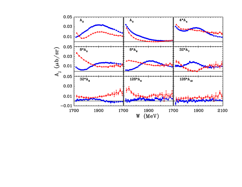
Figure 20: (Color online) Coefficients for associated Legendre functions of the second order for $\pi^{0}p$ (solid circles) and $\pi^{+}n$ (solid triangles). Solid lines are plotted to help guide the eye.

The photoproduction of a pseudoscalar meson is described by four independent helicity amplitudes which may be decomposed over Wigner harmonics $d^{j}_{\lambda\mu}(\theta)$. JW59 After Barker et al. BDS74 ; BDS75 , those amplitudes are commonly denoted $N$, $S_{1}$, $S_{2}$, and $D$, where $\mu=1/2$ and $\lambda=+1/2,-1/2,+3/2,-3/2$, respectively. The amplitude $N$ is the non-flip helicity amplitude, the $S$ amplitudes correspond to the single-flip helicity amplitudes, and the $D$ amplitude corresponds to the double-flip helicity amplitude. The beam asymmetry $\Sigma$ is related to these helicity amplitudes by the relation  BDS75

$$[\Sigma~{}d\sigma/d\Omega]\sim 2Re[S_{1}^{\ast}~{}S_{2}-N~{}D^{\ast}].$$ (22)

The first summand of this relation contains terms with products $d^{j_{1}}_{3/2,1/2}$ $d^{j_{2}}_{-1/2,1/2}$, while the second contains products $d^{j_{1}}_{1/2,1/2}$ $d^{j_{2}}_{-3/2,1/2}$. These products yield Clebsch-Gordan series over the associated second-order Legendre functions $P^{2}_{j}(\theta)$, with the degree $j$ given by $|j_{1}-j_{2}|\leq j\leq j_{1}+j_{2}$. JW59 The beam asymmetry as a whole, then, may be represented by an infinite series over these second-order associated Legendre functions of degree $j$, with the degree $j$ running from $j=$2 to infinity, after recalling that $j$ should not be less than 2.

We have used such a series to fit the data on the beam asymmetry $\Sigma$ reported here, supplemented by the fact that $\Sigma(0)$ = $\Sigma(\pi)$ = 0. The small statistical uncertainties of the data obtained here allow a correspondingly robust determination of the second-order associated Legendre function coefficients $A_{j}$; these coefficients were very difficult to determine unambiguously with previously published data of lower statistical accuracy. The results of our fits yield unprecedented detail on the energy dependence of the Legendre coefficients $A_{j}$, and should prove very useful in disentangling the helicity amplitudes associated with pion photoproduction for the present energy range.

As expected for such a fit using orthogonal polynomials, the Legendre coefficients $A_{j}$ decrease markedly for large $j$. At our energies and precision, a maximum value of $j$ = 10 was found to be sufficient to describe the data. Thus, we truncate the infinite series accordingly, using the relation

$$[\Sigma~{}d\sigma/d\Omega](\cos\theta)=\sum\limits_{j=2}^{10}(2j+1)~{}A_{j}~{}P^{2}_{j}(\cos\theta),$$

where the degree $j$ runs from 2 to 10.

In Fig. 20, we illustrate Legendre coefficients $A_{2}-A_{10}$ as a function of center-of-mass energy $W$ from the best fit of the product of the experimental CLAS $\Sigma$ data provided by this work and DU13 predictions for $d\sigma/d\Omega$. None of the coefficients show a narrow structure in the energy dependence. However, wide structures are clearly seen in the range W = 1.8 - 2.0 GeV, most likely attributable to contributions from one or more nucleon resonances known in this energy region with spins up to 7/2. PDG It is interesting that the coefficients $A_{3}$ for both final states have no energy structures at all; they are smooth functions throughout this energy region, with no evidence of the structures seen for the other coefficients.

For the $\pi^{+}n$ final state, the behavior of the $A_{j}$ is noticeably different for most of the coefficients than the behavior observed for the $\pi^{0}p$ final state. The energy dependence of the $A_{2}$ term for the $\pi^{+}n$ final state has a similar, though smaller, bump as seen in the neutral pion data. Likewise, the $A_{3}$ coefficients for both the $\pi^{+}n$ and $\pi^{0}p$ final states show similar energy behavior. The energy dependences of the $A_{4}$ - $A_{8}$ coefficients for the $\pi^{+}n$ final state are seen to lack the narrow structures seen for the $\pi^{0}p$ final state. Moreover, the $A_{8}$ coefficient for the neutral pion changes sign near W = 1950 MeV, while staying positive for the $\pi^{+}n$ case.

These pronounced differences between charged and neutral pion reactions reveal the essential role of the interferences between the photoproduction amplitudes for the two final states with isospin 1/2 and 3/2. Energy structures are less clear for the coefficients $A_{9}$ and $A_{10}$. The $A_{10}$ coefficients, especially for the neutral pion, are statistically consistent with zero, thus justifying our truncation of the Legendre series.

The pion production angles 60^∘ and 120^∘ are “mirror” angles which reveal dynamics associated with the interference of several amplitudes having different angular momenta. The sharpness of both dips seen in the $\Sigma$ data indicates that important contributions must come from partial waves with large $j$.

This analysis of the angular dependence of the beam asymmetry data in terms of associated Legendre functions reinforces the long-recognized complexity of the nucleon resonance spectrum in this energy region. That complexity underscores the point that an accurate interpretation of beam asymmetry in pion photoproduction will require a comprehensive account of the amplitude interference effects both in terms of angular momentum $j$ and isospin. The complicated interplay of the contributions from the different resonances demands further clarification through measurements of other polarization observables in order to isolate contributions to particular amplitudes. For example, the expression in equation 22 above for the beam asymmetry $\Sigma$ in terms of $N$, $S_{1}$, $S_{2}$, and $D$ from Ref. BDS75 may be compared to the expression from the same reference for the double-polarized observable $G$,

$$[G~{}d\sigma/d\Omega]\sim 2\rm{Im}[S_{1}^{\ast}~{}S_{2}-N~{}D^{\ast}].$$

Thus, the combination of $\Sigma$ and $G$ data greatly facilitate isolating the individual contributions of each helicity amplitude. New data on polarization observables have been taken (Ref. frostProp ) in Hall-B at Jefferson Laboratory using a polarized target (transverse and longitudinal) with polarized photon beams (circular and linear) that is currently undergoing analysis for the observables G, F, T, P. The information from these observables, coupled with the detailed results obtained here for $\Sigma$, will permit tremendous progress in deconvoluting the nucleon resonance spectrum.

XI Conclusion

An extensive and precise dataset (1086 data points) on the beam asymmetry $\Sigma$ for $\pi^{0}$ and $\pi^{+}$ photoproduction from the proton has been obtained, and a Fourier moment technique for extracting beam asymmetries from experimental data has been described. The measurements obtained here have been compared to existing data. The overall agreement is good, while the data provided here more than double the world database for both pion reactions, are more precise than previous measurements, and cover the reported energies with finer resolution.

The present data were found to favor the SAID and Bonn-Gatchina analyses over the older MAID predictions for both reactions. The present set of beam asymmetries has been incorporated into the SAID database, and exploratory fits have been made, resulting in a significant improvement in the fit chi-squared, and allowing for a much improved mapping of the sharp structure near $60^{\circ}$ and less sharp one near $120^{\circ}$ at photon energies greater than about 1600 MeV. Resonance couplings have been extracted and the largest change from previous fits was found to occur for the $\Delta(1700)3/2^{-}$ and $\Delta(1905)5/2^{+}$ states.

Beyond these phenomenological analyses, we performed an analysis of our beam asymmetry data using a series based on associated Legendre functions, coupled with predictions for the differential cross sections from SAID. This fit was made possible by the high statistical accuracy of the current data set. The analysis clearly shows the important role of interference contributions coming from the isospin 1/2 and 3/2 basis states to the $\pi^{0}$ and $\pi^{+}$ photoproduction reactions. When combined with future measurements of $G$, these data should greatly help attempts to disentangle the contributions of various resonances to the photoproduction process.