SSU-HEP-13/08 Relativistic corrections to the pair double heavy
diquark production in $e^{+}e^{-}$ annihilation

Abstract

On the basis of perturbative QCD and relativistic quark model we calculate relativistic and bound state corrections in the production processes of a pair of double heavy diquarks. Relativistic factors in the production amplitude connected with the relative motion of heavy quarks and the transformation law of the bound state wave function to the reference frame of the moving diquark $S$-wave bound states are taken into account. For the gluon and quark propagators entering the production vertex function we use a truncated expansion in the ratio of the relative quark momenta to the center-of-mass energy $s$ up to the second order. Relativistic corrections to the quark-quark bound state wave functions in the rest frame are considered by means of the Breit-like potential. It turns out that examined effects change essentially nonrelativistic results of the cross sections. The estimate of the yield of pairs of double heavy baryons $(ccq)$ at the B-factory is presented.

I Introduction

In last years the reactions of pair charmonium production in $e^{+}e^{-}$ annihilation have attracted considerable interest. A growth of the luminosity made it possible to observe experimentally at the Belle and BABAR Belle ; BaBar double $S$- and $P$-wave charmonium production. On the other hand, the defects of theoretical description of such processes on the basis of nonrelativistic QCD (NRQCD) were revealed and corrected BL1 ; bodwin ; Chao ; Qiao ; BLL ; EM2006 ; ji ; jia . Despite the evident successes achieved in this field on the basis of NRQCD BBL and potential quark models in correcting the discrepancy between the theory and experiment, the double charmonium production in $e^{+}e^{-}$ annihilation remains an interesting task. On the one hand, there are other production processes of orbitally excited charmonium states which can be investigated in the same way as the production of $S$-wave states. Several years ago the Belle and BABAR collaborations discovered new charmonium-like states in $e^{+}e^{-}$ annihilation pahlova ; brambilla-2011 . The nature of these numerous resonances remains unclear to the present. Some of them could be considered as a $D$-wave excitations in the system ($c\bar{c}$). On the other hand, the variety of the used approaches and model parameters in this problem raises a question about the comparison of obtained results that will lead to a better understanding of the quark-gluon dynamics and different mechanisms of double heavy quarkonium production. At last, the obtained luminosity on the meson B-factory ${\mathcal{L}}=10^{34}~{}cm^{-2}~{}c^{-1}$ allows to observe double heavy baryon $(ccq)$ production. In the threshold region of double heavy baryon production in $e^{+}e^{-}$ annihilation the double baryon production can give appreciable contribution to the cross section. For the estimate of such events yield in bkc it was performed a calculation of exclusive pair production of double heavy diquarks ($\bar{\cal D}$ and ${\cal D}$) in nonrelativistic approximation. It seems reasonably good guess that first stage of double heavy baryon production in $e^{+}e^{-}$ annihilation consists in the formation of the diquark nuclei $(Q_{1}Q_{2})$ and $(\bar{Q}_{1}\bar{Q}_{2})$ which are tightly bound, small size anti-triplet pairs. baryon_diquark ; gklo . In second stage the produced diquark and antidiquark join a light quark to produce the final baryons $(Q_{1}Q_{2}q)$ and $(\bar{Q}_{1}\bar{Q}_{2}\bar{q})$ if we neglect possible formation of ${\cal D}\bar{\cal D}$ bound states. Other baryon production mechanism in $e^{+}e^{-}$ annihilation connected with a production of $Q\bar{Q}$ pair and its subsequent fragmentation into the baryons was analyzed also in the literature brambilla-2011 ; baryon_diquark . So, the first stage of the process looks similar to the double charmonium production. It is clear that for it theoretical description we can use improved relativistic formalism as in the meson case EM2006 .

It is useful to remember that two sources of the change of nonrelativistic cross section for double charmonium production are revealed to the present: radiative corrections of order $O(\alpha_{s})$ and relative motion of $c$-quarks forming the bound states. An actual physical processes of charmonium production require a formation of hadronic particles in final states (bound states of a charm quark $c$ and a charm antiquark $\bar{c}$), for which perturbative quantum chromodynamics can not provide high precision description. In quark model a transition of free quarks to the mesons is described in terms of the bound state wave functions. Further investigation of exclusive heavy quark bound state production in $e^{+}e^{-}$ annihilation including relativistic effects by an example of diquarks can improve our understanding of a formation of quark bound states.

This work continues our study of the exclusive double charmonium production in $e^{+}e^{-}$ annihilation in the case of a diquark $(cc)$, $(bc)$ $S$-wave states on the basis of a relativistic quark model (RQM) EM2006 ; EFGM2009 ; EM2010 ; apm2005 ; rqm5 ; mt . Note that the term RQM specifies an approach in which the systematic account of corrections connected with relative motion of heavy quarks can be performed. Relativistic quark model provides a solution in many tasks of heavy quark physics. It uses a number of perturbative and nonperturbative parameters entering in the quark interaction operator. All observables can be expressed in terms of these parameters. In this way we can check the predictions of any quark model and draw a conclusion about its successfulness. At the same time the existence of a large number of different quark models which are sometimes very complicated for the practical use puts a question about the elaboration of the unified model containing generally accepted structural elements. Another approach to the heavy quark physics which does not contain the ambiguities of the quark models was formulated in BBL . As any other model of strong interactions of quarks and gluons the approach of NRQCD introduces in the theory a large number of matrix elements parameterizing nonperturbative dynamics of quarks and gluons bodwin ; BBL ; gremm . To a certain extent the microscopic picture of the quark-gluon interaction resident in quark models is changed by the global picture operating with the numerous nonperturbative matrix elements. The improved determination of color-singlet NRQCD matrix elements for $S$-wave charmonium is presented in bodwin . Their study evidently shows that the account of relative order $v^{2}$ corrections significantly increases the values of the matrix elements of leading order in $v$. The correspondence between parameters of quark models and NRQCD which can be established, opens the way for better understanding of quark-gluon interactions at small distances. In this sense both approaches complement each other and could reveal new aspects of color dynamics of quarks and gluons. Thus, the aim of this study consists in the extension of relativistic approach to the quarkonium production from Refs.EM2006 ; EFGM2009 ; EM2010 on the processes of exclusive pair diquark production $e^{+}+e^{-}\to{\mathcal{D}}+\bar{\mathcal{D}}$, investigation the role of relativistic corrections of order $v^{2}$ to the production amplitudes and cross sections and determination of the interrelationship with the predictions of NRQCD. Assuming that arising in $e^{+}e^{-}$ annihilation diquarks can fragment into double heavy baryons we use the obtained expressions of total cross sections for an estimate of the cross sections for the pair production of baryons.

II General formalism

In the ground state the diquarks are two-particle bound states of quarks in an antisymmetric color state with zero angular momentum, positive parity and definite flavor and spin. A diquark may be an axial vector (spin 1) or a scalar (spin 0). In the case of two identical quarks a diquark has a spin 1. The attractive forces between two quarks in antisymmetric color state lead to a formation of the bound system which can be described in quark model in a manner similar to the quark-antiquark states. A diquark constructed from two heavy quarks ($b$ and $c$) may be considered as a nucleus of double heavy baryon. The production of heavy quark bound states at different high energy reactions is an interesting physical process which is studied during many tenths of years brambilla-2011 ; braaten ; kramer ; brodsky2013 . It gives an opportunity to investigate the quark-gluon dynamics beginning from small distances where the perturbative QCD is applicable, to large distances where nonperturbative aspects of QCD become crucial. We investigate the exclusive diquark-antidiquark production in electron-positron annihilation in the lowest-order perturbative quantum chromodynamics. The final state consists of a pair of bound states $(bc)$ and $(\bar{b}\bar{c})$ with different spins in the case of different heavy quarks. The case of two identical quarks $(cc)$ or $(bb)$ leads to the production only a pair of axial vector diquarks. The diagrams that give contributions to the amplitude of a diquark pair production processes in leading order of the QCD coupling constant $\alpha_{s}$ are presented in Fig. 1. Two other diagrams can be obtained by corresponding permutations. There are two stages of double diquark production process. In the first stage, which is described by perturbative QCD, the virtual photon $\gamma^{\ast}$ and gluon $g^{\ast}$ produce two heavy quarks $(bc)$ and two heavy antiquarks $(\bar{b}\bar{c})$ with the following four-momenta:

Figure 1: The production amplitude of a pair of diquark states in $e^{+}e^{-}$ annihilation. ${\cal D}_{bc}$, $\bar{\cal D}_{\bar{b}\bar{c}}$ denote the diquark and antidiquark states composed from heavy quarks $b$ and $c$ and antiquark $\bar{b}$ and $\bar{c}$ correspondingly. Wavy line shows the virtual photon and dashed line corresponds to the gluon. $\Gamma$ is the production vertex function.

$$p_{1}=\eta_{11}P+p,~{}p_{2}=\eta_{12}P-p,~{}(p\cdot P)=0,~{}\eta_{1i}=\frac{M_{D_{bc}}^{2}\pm m_{1}^{2}\mp m_{2}^{2}}{2M_{D_{bc}}^{2}},$$ (1)

$$q_{1}=\eta_{21}Q+q,~{}q_{2}=\eta_{22}Q-q,~{}(q\cdot Q)=0,~{}\eta_{2i}=\frac{M_{\bar{D}_{\bar{b}\bar{c}}}^{2}\pm m_{1}^{2}\mp m_{2}^{2}}{2M_{\bar{D}_{\bar{b}\bar{c}}}^{2}}$$

where $M_{D_{bc}}$ is the mass of diquark consisting of quarks $b$ and $c$. $P(Q)$ are the total four-momenta, $p=L_{P}(0,{\bf p})$, $q=L_{P}(0,{\bf q})$ are the relative four-momenta obtained from the rest frame four-momenta $(0,{\bf p})$ and $(0,{\bf q})$ by the Lorentz transformation to the system moving with the momenta $P$, $Q$. The momenta $p_{1,2}$ of the heavy quarks $c$, $b$ and antiquarks $\bar{c}$, $\bar{b}$ are not on a mass shell: $p_{1,2}^{2}=\eta_{1i}^{2}P^{2}-{\bf p}^{2}=\eta_{1i}^{2}M_{D_{bc}}^{2}-{\bf p}^{2}\not=m_{1,2}^{2}$. An expressions (1) describe the symmetrical escape of heavy quarks and antiquarks from the mass shell. In the second nonperturbative stage, quark and antiquark pairs form double heavy diquarks.

Let consider the production amplitude of scalar and axial vector diquarks, which can be presented in the form rqm5 ; EM2006 ; EM2010 :

$${\cal M}(p_{-},p_{+},P,Q)=-\frac{8\pi^{2}\alpha}{3s^{2}}\sqrt{M_{D_{bc}}M_{\bar{D}_{\bar{b}\bar{c}}}}\bar{v}(p_{+})\gamma^{\beta}u(p_{-})\delta_{ij}\int\frac{d{\bf p}}{(2\pi)^{3}}\int\frac{d{\bf q}}{(2\pi)^{3}}\times$$ (2)

$$\times Sp\left\{\bar{\Psi}^{\cal S}_{D_{bc}}(p,P)\Gamma_{1}^{\beta\nu}(p,q,P,Q)\bar{\Psi}^{\cal AV}_{\bar{D}_{\bar{b}\bar{c}}}(q,Q)\gamma_{\nu}-\bar{\Psi}^{\cal S}_{D_{bc}}(-p,P)\Gamma_{2}^{\beta\nu}(p,q,P,Q)\bar{\Psi}^{\cal AV}_{\bar{D}_{\bar{b}\bar{c}}}(-q,Q)\gamma_{\nu}\right\},$$

where $s$ is the center-of-mass energy, a superscript ${\cal S}$ indicates a scalar diquark, a superscript ${\cal AV}$ indicates an axial vector diquark, $\alpha$ is the fine structure constant. $\Gamma_{1,2}$ are the vertex functions defined below. The transition of free quarks to diquark bound states is described by specific wave functions. Relativistic wave functions of scalar and axial vector diquarks accounting for the transformation from the rest frame to the moving one with four momenta $P$, $Q$ are

$$\bar{\Psi}^{\cal S}_{D_{bc}}(p,P) = \frac{\bar{\Psi}^{0}_{D_{bc}}({\bf p})}{\sqrt{\frac{\epsilon_{1}(p)}{m_{1}}\frac{(\epsilon_{1}(p)+m_{1})}{2m_{1}}\frac{\epsilon_{2}(p)}{m_{2}}\frac{(\epsilon_{2}(p)+m_{2})}{2m_{2}}}}\left[\frac{\hat{v}_{1}-1}{2}+\hat{v}_{1}\frac{{\bf p}^{2}}{2m_{2}(\epsilon_{2}(p)+m_{2})}-\frac{\hat{p}}{2m_{2}}\right]$$ (4)

$$\times\gamma_{5}(1+\hat{v}_{1})\left[\frac{\hat{v}_{1}+1}{2}+\hat{v}_{1}\frac{{\bf p}^{2}}{2m_{1}(\epsilon_{1}(p)+m_{1})}+\frac{\hat{p}}{2m_{1}}\right],$$

$$\bar{\Psi}^{\cal AV}_{\bar{D}_{\bar{b}\bar{c}}}(q,Q) = \frac{\bar{\Psi}^{0}_{\bar{D}_{\bar{b}\bar{c}}}({\bf q})}{\sqrt{\frac{\epsilon_{1}(q)}{m_{1}}\frac{(\epsilon_{1}(q)+m_{1})}{2m_{1}}\frac{\epsilon_{2}(q)}{m_{2}}\frac{(\epsilon_{2}(q)+m_{2})}{2m_{2}}}}\left[\frac{\hat{v}_{2}-1}{2}+\hat{v}_{2}\frac{{\bf q}^{2}}{2m_{1}(\epsilon_{1}(q)+m_{1})}+\frac{\hat{q}}{2m_{1}}\right]$$ (6)

$$\times\hat{\varepsilon}_{\cal AV}(Q,S_{z})(1+\hat{v}_{2})\left[\frac{\hat{v}_{2}+1}{2}+\hat{v}_{2}\frac{{\bf q}^{2}}{2m_{2}(\epsilon_{2}(q)+m_{2})}-\frac{\hat{q}}{2m_{2}}\right],$$

where the hat is a notation for the contraction of four vector with the Dirac matrices, $v_{1}=P/M_{D_{bc}}$, $v_{2}=Q/M_{\bar{D}_{\bar{b}\bar{c}}}$; $\varepsilon_{\cal AV}(Q,S_{z})$ is the polarization vector of the axial vector diquark, $\epsilon_{1,2}(p)=\sqrt{p^{2}+m_{1,2}^{2}}$ and $m_{1,2}$ are the masses of $c$ and $b$ quarks. The relativistic functions (4)-(6) and the vertex functions $\Gamma_{1,2}$ do not contain the $\delta({\bf p}^{2}-\eta_{1i}^{2}M_{D_{bc}}^{2}+m_{1,2}^{2})$. More complicated factor including the bound state wave function in the rest frame presented in Eqs. (4) and (6) plays the role of the $\delta$-function. This means that instead of the substitutions $M_{D_{bc}}=\epsilon_{1}({\bf p})+\epsilon_{2}({\bf p})$ and $M_{\bar{D}_{\bar{b}\bar{c}}}=\epsilon_{1}({\bf q})+\epsilon_{2}({\bf q})$ in the production amplitude we carry out the integration over the quark relative momenta ${\bf p}$ and ${\bf q}$. Color part of the diquark wave function in the amplitude (2) is taken as $\epsilon_{ijk}/\sqrt{2}$ (color indexes $i,j,k=1,2,3$), so that general color factor in (2) is equal to $\delta_{ij}$. Relativistic wave functions in Eqs. (4) and (6) are equal to the product of wave functions in the rest frame $\Psi^{0}_{D_{bc}}$ and spin projection operators that are accurate at all orders in $|{\bf p}|/m$ rqm5 ; EM2006 . An expression of spin projector in different form has been derived primarily in Bodwin2002 where spin projectors are written in terms of heavy quark momenta $p_{1,2}$ lying on the mass shell. Our derivation of relations (4) and (6) accounts for the transformation law of the bound state wave functions from the rest frame to the moving one with four momenta $P$ and $Q$. This transformation law was discussed in the Bethe-Salpeter approach in BP and in quasipotential method in F1973 . We use the last one and write necessary transformation as follows:

$$\Psi_{P}^{\rho\omega}({\bf p})=D_{1}^{1/2,~{}\rho\alpha}(R^{W}_{L_{P}})D_{2}^{1/2,~{}\omega\beta}(R^{W}_{L_{P}})\Psi_{0}^{\alpha\beta}({\bf p}),$$ (7)

$$\bar{\Psi}_{P}^{\lambda\sigma}({\bf p})=\bar{\Psi}^{\varepsilon\tau}_{0}({\bf p})D_{1}^{+~{}1/2,~{}\varepsilon\lambda}(R^{W}_{L_{P}})D_{2}^{+~{}1/2,~{}\tau\sigma}(R^{W}_{L_{P}}),$$

where $R^{W}$ is the Wigner rotation, $L_{P}$ is the Lorentz boost from the diquark rest frame to a moving one, and the rotation matrix $D^{1/2}(R)$ is defined by

$${1\ \ \,0\choose 0\ \ \,1}D^{1/2}_{1,2}(R^{W}_{L_{P}})=S^{-1}({\bf p}_{1,2})S({\bf P})S({\bf p}),$$ (8)

where explicit form for the Lorentz transformation matrix of four-spinor is

$$S({\bf p})=\sqrt{\frac{\epsilon(p)+m}{2m}}\left(1+\frac{(\bm{\alpha}{\bf p})}{\epsilon(p)+m}\right).$$ (9)

We omit here intermediate expressions giving rise to our final relations (2)-(6) EM2006 ; EFGM2009 . The presence of the $\delta(p\cdot P)$ function allows to make the integration over relative energy $p^{0}$ if we write the initial production amplitude as a convolution of the truncated amplitude with two Bethe-Salpeter (BS) diquark wave functions. In the rest frame of a bound state the condition $p^{0}=0$ allows to eliminate the relative energy from the BS wave function. The BS wave function satisfies a two-body bound state equation which is very complicated and has no known solution. A way to deal with this problem is to find a soluble lowest-order equation containing main physical properties of the exact equation and develop a perturbation theory. For this purpose we continue to work in three-dimensional quasipotential approach. In this framework the double diquark production amplitude (2) can be written initially as a product of the production vertex function $\Gamma_{1,2}$ projected onto the positive energy states by means of the Dirac bispinors (free quark wave functions) and a bound state quasipotential wave functions describing diquarks in the reference frames moving with four momenta $P,Q$. Further transformations include the known transformation law of the bound state wave functions to the rest frame (7). The physical interpretation of the double diquark production amplitude is the following: we have a complicated transition of two heavy quark and antiquark which are produced in $e^{+}e^{-}$-annihilation outside the mass shell and their subsequent evolution firstly on the mass shell (free Dirac bispinors) and then to the quark bound states. In the spin projectors we have ${\bf p}^{2}\not=\eta_{1i}^{2}M^{2}-m_{1,2}^{2}$ just the same as in the vertex production functions $\Gamma_{1,2}$. We can not say exactly whether heavy quarks are on-shell or not in the spin projectors (4)-(6) because we should consider these structures as a transition form factors for heavy quarks from free states to bound states. In the course of the ${\cal M}$ transformation we introduce symmetrical spin wave functions for vector and scalar diquarks baryon_diquark ; hussain :

$$u_{i}(0)u_{j}(0)=\left[\frac{(1+\gamma_{0})}{2\sqrt{2}}\hat{\varepsilon}_{\cal AV}(\gamma_{5})C\right]_{ij},~{}~{}~{}v_{i}(0)v_{j}(0)=\left[\frac{(1-\gamma_{0})}{2\sqrt{2}}\hat{\varepsilon}_{\cal AV}(\gamma_{5})C\right]_{ij},$$ (10)

where $C$ is the charge conjugation matrix. As the color wavefunction of identical quarks $(cc)$ or $(bb)$ is antisymmetric and the quarks are taken to be in the ground state $S$-wave, the spin wave function must be symmetric. So, the $(cc)$ or $(bb)$ pair can only form a spin 1 diquark.

At leading order in $\alpha_{s}$ the vertex functions $\Gamma_{1,2}^{\beta\nu}(p,P;q,Q)$ can be written as ($\Gamma_{2}^{\beta\nu}(p,P;q,Q)$ can be obtained from $\Gamma_{1}^{\beta\nu}(p,P;q,Q)$ by means of the replacement $p_{1}\leftrightarrow p_{2}$, $q_{1}\leftrightarrow q_{2}$, $\alpha_{b}\to\alpha_{c}$, $Q_{c}\to Q_{b}$)

$$\Gamma_{1}^{\beta\nu}(p,P;q,Q)=Q_{c}\alpha_{b}\left[\gamma_{\mu}\frac{(\hat{l}-\hat{q}_{1}+m_{1})}{(l-q_{1})^{2}-m_{1}^{2}+i\epsilon}\gamma_{\beta}D^{\mu\nu}(k_{2})+\gamma_{\beta}\frac{(\hat{p}_{1}-\hat{l}+m_{1})}{(p_{1}-l)^{2}-m_{1}^{2}+i\epsilon}\gamma_{\mu}D^{\mu\nu}(k_{2})\right],$$ (11)

$$\Gamma_{2}^{\beta\nu}(p,P;q,Q)=Q_{b}\alpha_{c}\left[\gamma_{\mu}\frac{(\hat{l}-\hat{q}_{2}+m_{2})}{(l-q_{2})^{2}-m_{2}^{2}+i\epsilon}\gamma_{\beta}D^{\mu\nu}(k_{1})+\gamma_{\beta}\frac{(\hat{p}_{2}-\hat{l}+m_{2})}{(p_{2}-l)^{2}-m_{2}^{2}+i\epsilon}\gamma_{\mu}D^{\mu\nu}(k_{1})\right],$$ (12)

where the gluon momenta are $k_{1}=p_{1}+q_{1}$, $k_{2}=p_{2}+q_{2}$ and $l^{2}=s^{2}=(P+Q)^{2}=(p_{-}+p_{+})^{2}$, $\alpha_{c,b}=\alpha_{s}\left(\frac{m_{1,2}^{2}}{M^{2}}s^{2}\right)$, $p_{-}$, $p_{+}$ are four momenta of the electron and positron. The dependence on the relative momenta of heavy quarks is presented both in the gluon propagator $D_{\mu\nu}(k)$ and quark propagator as well as in relativistic wave functions (4) and (6). Taking into account that the ratio of relative quark momenta $p$ and $q$ to the energy $s$ is small, we expand inverse denominators of quark and gluon propagators as follows:

$$\frac{1}{(l-q_{1,2})^{2}-m_{1,2}^{2}}=\frac{1}{r_{2,1}s^{2}}\left[1-\tilde{B}_{AV}\frac{(2r_{1,2}-1)}{r_{2,1}}-\frac{2r_{1,2}M^{2}}{s^{2}}(\tilde{B}_{S}-r_{1,2}\tilde{B}_{AV})-\frac{(q^{2}\mp 2lq)}{r_{2,1}s^{2}}+\cdots\right],$$ (13)

$$\frac{1}{(l-p_{1,2})^{2}-m_{1,2}^{2}}=\frac{1}{r_{2,1}s^{2}}\left[1-\tilde{B}_{S}\frac{(2r_{1,2}-1)}{r_{2,1}}-\frac{2r_{1,2}M^{2}}{r_{2,1}s^{2}}(\tilde{B}_{AV}-r_{1,2}\tilde{B}_{S})-\frac{(p^{2}\mp 2lp)}{r_{2,1}s^{2}}+\cdots\right],$$ (14)

$$\frac{1}{k_{1,2}^{2}}=\frac{1}{r_{2,1}^{2}s^{2}}\left[1-\frac{(1-2r_{2,1})}{r_{2,1}}(\tilde{B}_{S}+\tilde{B}_{AV})\pm\frac{2(pQ+qP)}{r_{2,1}s^{2}}-\frac{(p^{2}+q^{2}+2pq)}{r^{2}_{2,1}s^{2}}+\cdots\right],$$ (15)

where $B_{S}$ and $B_{AV}$ are the bound state energies of scalar and vector diquarks, $\tilde{B}_{S,AV}=B_{S,AV}/(m_{1}+m_{2})$, $M=m_{1}+m_{2}$, $r_{1,2}=m_{1,2}/M$. Substituting (13)-(15), (4)-(6) in (2) we preserve relativistic factors entering the denominators of relativistic wave functions (4) and (6), but in the numerator of the amplitude (2) we take into account corrections of second order in $|{\bf p}|/m_{1,2}$ and $|{\bf q}|/m_{1,2}$ relative to the leading order result. This provides the convergence of resulting momentum integrals. Calculating the trace in the amplitude (2) by means of the system FORM FORM , we find that relativistic amplitudes describing the production of diquark pairs have the following structure:

$${\cal M}_{SS}=-\frac{128\pi^{2}\alpha}{3s^{6}}\frac{M^{5}}{r_{1}^{2}r_{2}^{2}M_{D_{bc}}^{3}}(v_{2}-v_{1})^{\beta}\bar{v}(p_{+})\gamma_{\beta}u(p_{-})\delta_{ij}\bar{\Psi}^{0}_{SD_{bc}}(0)\bar{\Psi}^{0}_{S\bar{D}_{\bar{b}\bar{c}}}(0)\times$$ (16)

$$\left[\frac{Q_{c}\alpha_{s}(\frac{m_{2}^{2}}{M^{2}}s^{2})}{r_{2}^{3}}F_{1,S}+\frac{Q_{b}\alpha_{s}(\frac{m_{1}^{2}}{M^{2}}s^{2})}{r_{1}^{3}}F_{2,S}\right]$$

$${\cal M}_{SAV}=-\frac{128\pi^{2}\alpha}{3s^{6}}\frac{M^{5}}{M_{D_{bc}}^{3/2}M_{\bar{D}_{\bar{b}\bar{c}}}^{3/2}}\varepsilon_{\beta\alpha\sigma\lambda}\varepsilon_{\cal AV}^{\alpha}v_{1}^{\sigma}v_{2}^{\lambda}\bar{v}(p_{+})\gamma_{\beta}u(p_{-})\delta_{ij}\bar{\Psi}^{0}_{SD_{bc}}(0)\bar{\Psi}^{0}_{AV\bar{D}_{\bar{b}\bar{c}}}(0)\times$$ (17)

$$\left[\frac{Q_{c}\alpha_{s}(\frac{m_{2}^{2}}{M^{2}}s^{2})}{r_{2}^{3}}F_{1,SAV}-\frac{Q_{b}\alpha_{s}(\frac{m_{1}^{2}}{M^{2}}s^{2})}{r_{1}^{3}}F_{2,SAV}\right],$$

$${\cal M}_{AVAV}=-\frac{128\pi^{2}\alpha}{3s^{6}}\frac{M^{5}}{r_{1}^{2}r_{2}^{2}M_{D_{bc}}^{3}}\bar{v}(p_{+})\gamma_{\beta}u(p_{-})\delta_{ij}\bar{\Psi}^{0}_{AVD_{bc}}(0)\bar{\Psi}^{0}_{AV\bar{D}_{\bar{b}\bar{c}}}(0)\Bigl{[}F_{1,AV}(v_{2}-v_{1})^{\beta}(\varepsilon_{1,{\cal AV}}\cdot\varepsilon_{2,{\cal AV}})+$$

$$+F_{2,AV}(v_{2}-v_{1})^{\beta}(\varepsilon_{1,{\cal AV}}\cdot v_{2})(\varepsilon_{2,{\cal AV}}\cdot v_{1})+F_{3,AV}\left[(\varepsilon_{2,{\cal AV}}\cdot v_{1})\varepsilon^{\beta}_{1,{\cal AV}}-(\varepsilon_{1,{\cal AV}}\cdot v_{2})\varepsilon^{\beta}_{2,{\cal AV}}\right]\Bigr{]},$$ (18)

where $\varepsilon_{1,2,{\cal AV}}$ are the polarization vectors of spin 1 diquarks. The coefficient functions $F_{i,S}$, $F_{i,SAV}$, $F_{i,AV}$ can be presented as sums of terms containing specific relativistic factors $C_{ij}=[(m_{1}-\epsilon_{1}(p))/(m_{1}+\epsilon_{1}(p))]^{i}[(m_{2}-\epsilon_{2}(q))/(m_{2}+\epsilon_{2}(q))]^{j}$ with $i+j\leq 2$. Used analytical expressions for these functions are written explicitly in Appendix A. Introducing the scattering angle $\theta$ between the electron momentum ${\bf p}_{e}$ and momentum ${\bf P}$ of diquark $D_{bc}$, we can calculate the differential cross section $d\sigma/d\cos\theta$ and then the total cross section $\sigma$ as a function of center-of-mass energy $s$, masses of quarks and diquarks and relativistic parameters presented below. We find it useful to write double heavy diquark production differential cross sections in the following form:

$$\frac{d\sigma_{SS}}{d\cos\theta}=\frac{256\pi^{3}\alpha^{2}}{3s^{10}}\frac{M^{8}}{M_{D_{bc}}^{6}r_{1}^{4}r_{2}^{4}}|\bar{\Psi}^{0}_{SD_{bc}}(0)|^{2}|\bar{\Psi}_{{S\bar{D}}_{\bar{b}\bar{c}}}(0)|^{2}\left(1-\frac{4M^{2}_{D_{bc}}}{s^{2}}\right)^{3/2}\left(1-\cos^{2}\theta\right)\times$$ (19)

$$\left[\frac{Q_{c}\alpha_{s}(\frac{m_{2}^{2}}{M^{2}}s^{2})}{r_{2}^{3}}F_{1,S}+\frac{Q_{b}\alpha_{s}(\frac{m_{1}^{2}}{M^{2}}s^{2})}{r_{1}^{3}}F_{2,S}\right]^{2},$$

$$\frac{d\sigma_{SAV}}{d\cos\theta}=\frac{64\pi^{3}\alpha^{2}}{3s^{8}}\frac{M^{6}}{M_{D_{bc}}^{3}M_{\bar{D}_{\bar{b}\bar{c}}}^{3}}\left[\left(1-\frac{(M_{D_{bc}}+M_{\bar{D}_{\bar{b}\bar{c}}})^{2}}{s^{2}}\right)\left(1-\frac{(M_{D_{bc}}-M_{\bar{D}_{\bar{b}\bar{c}}})^{2}}{s^{2}}\right)\right]^{3/2}\times$$ (20)

$$|\bar{\Psi}^{0}_{SD_{bc}}(0)|^{2}|\bar{\Psi}_{{AV\bar{D}}_{\bar{b}\bar{c}}}(0)|^{2}\left[\frac{Q_{c}\alpha_{s}\left(\frac{m_{2}^{2}}{M^{2}}s^{2}\right)}{r_{2}^{3}}F_{1,SAV}-\frac{Q_{b}\alpha_{s}\left(\frac{m_{1}^{2}}{M^{2}}s^{2}\right)}{r_{1}^{3}}F_{2,SAV}\right]^{2}\left(2-\sin^{2}\theta\right),$$

$$\frac{d\sigma_{AVAV}}{d\cos\theta}=\frac{64\pi^{3}\alpha^{2}}{3s^{10}}\frac{M^{8}}{M_{D_{bc}}^{6}r_{1}^{4}r_{2}^{4}}|\bar{\Psi}^{0}_{AVD_{bc}}(0)|^{4}\left(1-\frac{4M^{2}_{D_{bc}}}{s^{2}}\right)^{3/2}\left(F_{A}-F_{B}\cdot\cos^{2}\theta\right),$$ (21)

$$F_{A}=F^{2}_{1,AV}(12-4\eta+\eta^{2})+F_{1,AV}F_{2,AV}(8\eta-6\eta^{2}+\eta^{3})+F_{1,AV}F_{3,AV}(4\eta-2\eta^{2})+$$

$$+F^{2}_{2,AV}(4\eta^{2}-2\eta^{3}+\frac{1}{4}\eta^{4})+F_{2,AV}F_{3,AV}(4\eta^{2}-\eta^{3})+F^{2}_{3,AV}(2\eta+\eta^{2}),$$

$$F_{B}=F^{2}_{1,AV}(12-4\eta+\eta^{2})+F_{1,AV}F_{2,AV}(8\eta-6\eta^{2}+\eta^{3})+F_{1,AV}F_{3,AV}(4\eta-2\eta^{2})+$$

$$+F^{2}_{2,AV}(4\eta^{2}-2\eta^{3}+\frac{1}{4}\eta^{4})+F_{2,AV}F_{3,AV}(4\eta^{2}-\eta^{3})+F^{2}_{3,AV}(-2\eta+\eta^{2}),$$

where $\eta=s^{2}/M^{2}_{D_{bc}}$, the values of wave function at the origin are equal

$$\Psi^{0}_{S,AVD_{bc}}(0)=\int\sqrt{\frac{(\epsilon_{1}(p)+m_{1})(\epsilon_{2}(p)+m_{2})}{2\epsilon_{1}(p)\cdot 2\epsilon_{2}(p)}}\Psi^{0}_{S,AVD_{bc}}({\bf p})\frac{d{\bf p}}{(2\pi)^{3}}.$$ (22)

This form of differential cross sections is very close to nonrelativistic form obtained in bkc . In nonrelativistic limit our results coincide with the calculations made in bkc excepting the cross section (21), which differs by the factor $1/8$ from bkc . The functions $F_{i,S}$, $F_{i,SAV}$ and $F_{i,AV}$ are obtained as series in $|{\bf p}|/m_{1,2}$ and $|{\bf q}|/m_{1,2}$ up to corrections of second order. Relativistic parameters $\omega^{S,AV}_{nk}$ entering in $F_{i,S}$, $F_{i,SAV}$ and $F_{i,AV}$ (see Appendix A) can be expressed in terms of momentum integrals $I_{nk}$ as follows:

$$I_{nk}^{S,AV}=\int_{0}^{\infty}q^{2}R^{S,AV}_{D_{bc}}(q)\sqrt{\frac{(\epsilon_{1}(q)+m_{1})(\epsilon_{2}(q)+m_{2})}{2\epsilon_{1}(q)\cdot 2\epsilon_{2}(q)}}\left(\frac{m_{1}-\epsilon_{1}(q)}{m_{1}+\epsilon_{1}(q)}\right)^{n}\left(\frac{m_{2}-\epsilon_{2}(q)}{m_{2}+\epsilon_{2}(q)}\right)^{k}dq,$$ (23)

$$\omega^{S,AV}_{10}=\frac{I^{S,AV}_{10}}{I^{S,AV}_{00}},~{}\omega^{S,AV}_{01}=\frac{I^{S,AV}_{01}}{I^{S,AV}_{00}},~{}\omega^{S,AV}_{11}=\frac{I^{S,AV}_{11}}{I^{S,AV}_{00}},~{}\omega^{S,AV}_{20}=\frac{I^{S,AV}_{20}}{I^{S,AV}_{00}},~{}\omega^{S,AV}_{02}=\frac{I^{S,AV}_{02}}{I^{S,AV}_{00}}.$$ (24)

On the one hand, in the potential quark model relativistic corrections, connected with relative motion of heavy quarks, enter the production amplitude (2) and the cross sections (19), (20) and (21) through the different relativistic factors. They are determined in final expressions by specific parameters $\omega^{S,AV}_{nk}$. The momentum integrals which determine the parameters $\omega^{S,AV}_{nk}$ are convergent and we can calculate them numerically, using the wave functions obtained by the numerical solution of the Schrödinger equation. Nevertheless, we introduce new cutoff parameter $\Lambda\approx m_{c}$ for momentum integrals $I_{nk}$ in (23) at high momenta $q$ because we don’t know exactly the bound state wave functions in the region of the relativistic momenta.

The exact form of the wave functions $\Psi^{0}_{SD_{bc}}({\bf q})$ and $\Psi^{0}_{AVD_{bc}}({\bf q})$ is important to improve an accuracy of the calculation of relativistic effects. In nonrelativistic approximation double diquark production cross sections (19), (20) and (21) contain fourth power of nonrelativistic wave function at the origin. Small changes of $\Psi^{0}_{S,AVD_{bc}}$ lead to substantial changes of final results. In the framework of NRQCD this problem is closely related to the determination of color-singlet matrix elements for heavy quarkonium BBL . Thus, on the other hand, there are relativistic corrections to the bound state wave functions of scalar and axial vector diquarks. In order to take them into account, we suppose that the dynamics of a $(bc)$-pair is determined by the QCD generalization of the standard Breit Hamiltonian in the center-of-mass reference frame repko1 ; pot1 ; pot3 ; capstick :

$$H=H_{0}+\Delta U_{1}+\Delta U_{2},~{}~{}~{}H_{0}=\sqrt{{\bf p}^{2}+m_{1}^{2}}+\sqrt{{\bf p}^{2}+m_{2}^{2}}-\frac{2\tilde{\alpha}_{s}}{3r}+\frac{1}{2}(Ar+B),$$ (25)

$$\Delta U_{1}(r)=-\frac{\alpha_{s}^{2}}{6\pi r}\left[2\beta_{0}\ln(\mu r)+a_{1}+2\gamma_{E}\beta_{0}\right],~{}~{}a_{1}=\frac{31}{3}-\frac{10}{9}n_{f},~{}~{}\beta_{0}=11-\frac{2}{3}n_{f},$$ (26)

$$\Delta U_{2}(r)=-\frac{\alpha_{s}}{3m_{1}m_{2}r}\left[{\bf p}^{2}+\frac{{\bf r}({\bf r}{\bf p}){\bf p}}{r^{2}}\right]+\frac{\pi\alpha_{s}}{3}\left(\frac{1}{m_{1}^{2}}+\frac{1}{m_{2}^{2}}\right)\delta({\bf r})+\frac{2\alpha_{s}}{3r^{3}}\left(\frac{1}{2m_{1}^{2}}+\frac{1}{m_{1}m_{2}}\right)({\bf S}_{1}{\bf L})+$$ (27)

$$+\frac{2\alpha_{s}}{3r^{3}}\left(\frac{1}{2m_{2}^{2}}+\frac{1}{m_{1}m_{2}}\right)({\bf S}_{2}{\bf L})+\frac{16\pi\alpha_{s}}{9m_{1}m_{2}}({\bf S}_{1}{\bf S}_{2})\delta({\bf r})+\frac{2\alpha_{s}}{m_{1}m_{2}r^{3}}\left[\frac{({\bf S}_{1}{\bf r})({\bf S}_{2}{\bf r})}{r^{2}}-\frac{1}{3}({\bf S}_{1}{\bf S}_{2})\right]-$$

$$-\frac{\alpha_{s}^{2}(m_{1}+m_{2})}{2m_{1}m_{2}r^{2}}\left[1-\frac{4m_{1}m_{2}}{9(m_{1}+m_{2})^{2}}\right],$$

where ${\bf L}=[{\bf r}\times{\bf p}]$, ${\bf S}_{1}$, ${\bf S}_{2}$ are spins of heavy quarks, $n_{f}$ is the number of flavors, $\gamma_{E}\approx 0.577216$ is the Euler constant. To describe the hyperfine splittings in $(b\bar{c})$ and $(c\bar{c})$ mesons (and $S$-wave diquark system) which could be in agreement with experimental data and other calculations in quark models we add to the standard Breit potential the spin confining potentials obtained in repko1 ; repko2 :

$$\Delta V^{hfs}_{conf}(r)=f_{V}\frac{A}{8r}\left\{\frac{1}{m_{1}^{2}}+\frac{1}{m_{2}^{2}}+\frac{16}{3m_{1}m_{2}}({\bf S}_{1}{\bf S}_{2})+\frac{4}{3m_{1}m_{2}}\left[3({\bf S}_{1}{\bf r})({\bf S}_{2}{\bf r})-({\bf S}_{1}{\bf S}_{2})\right]\right\},$$ (28)

where we take the parameter $f_{V}=0.9$. For the dependence of the QCD coupling constant $\tilde{\alpha}_{s}(\mu^{2})$ on the renormalization point $\mu^{2}$ in the pure Coulomb term in (25) we use the three-loop result kniehl1997

$$\tilde{\alpha}_{s}(\mu^{2})=\frac{4\pi}{\beta_{0}L}-\frac{16\pi b_{1}\ln L}{(\beta_{0}L)^{2}}+\frac{64\pi}{(\beta_{0}L)^{3}}\left[b_{1}^{2}(\ln^{2}L-\ln L-1)+b_{2}\right],\quad L=\ln(\mu^{2}/\Lambda^{2}),$$ (29)

whereas in other terms of the Hamiltonians (26) and (27) we take the leading order approximation. The typical momentum transfer scale in a quarkonium is of order of double reduced mass, so we set the renormalization scale $\mu=2m_{1}m_{2}/(m_{1}+m_{2})$ and $\Lambda=0.168$ GeV, which gives $\alpha_{s}=0.314$ for diquark $(cc)$, $\alpha_{s}=0.265$ for diquark $(bc)$. The coefficients $b_{i}$ are written explicitly in kniehl1997 . The parameters of the linear potential $A=0.18$ GeV² and $B=-0.16$ GeV have usual values of quark models.

Table 1: Numerical values of relativistic parameters (24) in double heavy diquark production cross sections (19), (20), (21).

Diquarks	$n^{2S+1}L_{J}$	$M_{D}$,	$\Psi^{0}_{S,AVD}(0)$,	$\omega^{S,AV}_{10}$	$\omega^{S,AV}_{01}$	$\omega^{S,AV}_{11}$	$\omega^{S,AV}_{02}$	$\omega^{S,AV}_{20}$
$(bc)$, $(cc)$,		GeV	GeV3/2
$SD_{bc}$	$1^{1}S_{0}$	6.349	0.148	-0.0454	-0.0054	0.00048	0.00006	0.0039
$AVD_{bc}$	$1^{3}S_{1}$	6.362	0.136	-0.0467	-0.0055	0.00048	0.00006	0.0039
$AVD_{cc}$	$1^{3}S_{1}$	3.339	0.114	-0.0431	-0.0431	0.0033	0.0033	0.0033

Table 2: The comparison of obtained results for the production cross sections with nonrelativistic calculation. In third column we present nonrelativistic result obtained in our model pointing out the Ref.bkc where nonrelativistic approximation of the cross sections was discussed for the first time.

Final state $D_{1}D_{2}$	Center-of-mass energy s	$\sigma_{NR}$, bkc	Our result $\sigma_{R}$
$SD_{bc}+S\bar{D}_{\bar{b}\bar{c}}$	15.0 GeV	0.0009 fb	0.0011 fb
$SD_{bc}+AV\bar{D}_{\bar{b}\bar{c}}$	16.0 GeV	0.070 fb	0.034 fb
$AVD_{bc}+AV\bar{D}_{\bar{b}\bar{c}}$	16.0 GeV	0.178 fb	0.072 fb
$AVD_{cc}+AV\bar{D}_{\bar{c}\bar{c}}$	7.6 GeV	0.378 fb	0.095 fb
$AVD_{cc}+AV\bar{D}_{\bar{c}\bar{c}}$	10.6 GeV	0.070 fb	0.025 fb

For the calculation of relativistic corrections in the bound state diquark wave functions $\Psi^{0}_{S,AVD_{bc}}({\bf p})$ we take the Breit potential (25) and construct the effective potential model as in EM2010 ; Lucha by means of the rationalization of kinetic energy operator. Using the program of numerical solution of the Schrödinger equation LS we obtain the values of all relativistic parameters entering the cross sections (19), (20) and (21) which are collected in Table 1. There is no free diquark to study the effective interaction between two heavy quarks. So, as a test calculation for our model we find the masses of charmonium states and $B_{c}$ mesons which are in good agreement with experimental data and other calculations in quark models. For example, in the case of low lying $(b\bar{c})$ mesons we obtain $M(B_{c}^{\pm})=M(1^{1}S_{0})=6.280$ GeV and $M(1^{3}S_{1})=6.322$ GeV. Numerical data related with charmonium states are discussed in EM2010 . Strictly speaking we can obtain the charmonium mass spectrum which agrees with experimental data with more than a per cent accuracy EM2010 ; PDG . Our masses of $S$-wave diquarks $(bc)$ and $(cc)$ in nonrelativistic approximation are 6.608 GeV and 3.328 GeV correspondingly. In gklo a diquark $(bc)$ ($1S$-state) has the mass 6.48 GeV and diquark $(cc)$ ($1S$-state) 3.16 GeV. The difference between gklo and our results amounts near 2 and 4 per cents and is related with the different value of $c$-quark mass in gklo . An account of relativistic corrections in our model leads to slightly different values: the mass of $(bc)$ diquark is 6.349 GeV ($S$=0-state), 6.362 GeV ($S$=1-state) and mass of $(cc)$ diquark is 3.339 GeV ($S$=1-state). The difference in $3\div 4$ per cents occurs in comparison with our results in baryon_diquark where different approach to the calculation of relativistic corrections is used. The values of diquark $(bc)$ and $(cc)$ wave functions at the origin in gklo $\Psi_{bc}(0)=0.205~{}GeV^{3/2}$ and $\Psi_{cc}(0)=0.150~{}GeV^{3/2}$ are in the agreement with our nonrelativistic results $\Psi^{0}_{D_{bc}}(0)=0.185~{}GeV^{3/2}$ and $\Psi^{0}_{D_{cc}}(0)=0.145~{}GeV^{3/2}$. Then we calculate the parameters of diquark states and production cross sections as functions of center-of-mass energy $s$. The total cross section plots for the production of diquarks $(bc)$ and $(cc)$ are presented in Fig. 2. In Table 2 we give numerical values of total production cross sections at certain center-of-mass energies $s$ and compare them with nonrelativistic result in our quark model. These numerical results could be considered as an estimate for the experimental search.

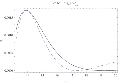
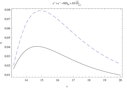
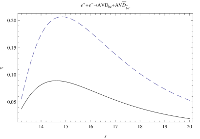
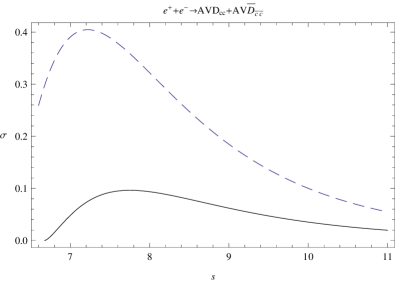
Figure 2: The cross section in fb of $e^{+}e^{-}$ annihilation into a pair of $S$-wave scalar and axial vector diquark states $(bc)$ and axial vector diquark state $(cc)$ as a function of the center-of-mass energy $s$ (solid line). The dashed line shows nonrelativistic result without bound state and relativistic corrections.

III Numerical results and discussion

In this paper we have investigated the role of relativistic and bound state effects in the production processes of a pair double heavy diquarks in the quark model. We calculate relativistic effects taking into account their important role in the exclusive pair production of charmonium states in $e^{+}e^{-}$ annihilation. By the construction of the production amplitude (2) we keep relativistic corrections of two types. The first type is determined by several functions depending on the relative quark momenta ${\bf p}$ and ${\bf q}$ arising from the gluon propagator, the quark propagator and the relativistic diquark wave functions. The second type of corrections originates from the perturbative and nonperturbative treatment of the quark-quark interaction operator which leads to the different wave functions $\Psi^{0}_{S,AVD_{bc}}({\bf p})$ and $\Psi^{0}_{S,AV\bar{D}_{\bar{b}\bar{c}}}({\bf q})$ for the diquark bound states. In addition, we systematically accounted for the bound state corrections working with the masses of diquark bound states or with the bound state energies $B_{S}$, $B_{AV}$. The calculated masses of diquark states agree well with previous theoretical results baryon_diquark . Note that basic parameters of the model are kept fixed from previous calculations of the meson mass spectra and decay widths rqm5 ; rqm1 ; brambilla-2011 ; QWG .

It follows from the results (19), (20), (21) that the total cross sections for the exclusive pair production of scalar, scalar+axial vector, axial vector diquarks in $e^{+}e^{-}$ annihilation can be presented in the form:

$$\sigma_{SS}=\frac{1024\pi^{3}\alpha^{2}}{9s^{10}}\frac{M^{8}}{r_{1}^{4}r_{2}^{4}M^{6}_{D_{bc}}}|\bar{\Psi}^{0}_{SD_{bc}}(0)|^{4}\left(1-\frac{4M^{2}_{D_{bc}}}{s^{2}}\right)^{3/2}\left[\frac{Q_{c}\alpha_{s}(\frac{m_{2}^{2}}{M^{2}}s^{2})}{r_{2}^{3}}F_{1,S}+\frac{Q_{b}\alpha_{s}(\frac{m_{1}^{2}}{M^{2}}s^{2})}{r_{1}^{3}}F_{2,S}\right]^{2},$$ (30)

$$\sigma_{SAV}=\frac{512\pi^{3}\alpha^{2}}{9s^{8}}\frac{M^{6}}{M_{D_{bc}}^{3}M_{\bar{D}_{\bar{b}\bar{c}}}^{3}}\left[\left(1-\frac{(M_{D_{bc}}+M_{\bar{D}_{\bar{b}\bar{c}}})^{2}}{s^{2}}\right)\left(1-\frac{(M_{D_{bc}}-M_{\bar{D}_{\bar{b}\bar{c}}})^{2}}{s^{2}}\right)\right]^{3/2}\times$$ (31)

$$|\bar{\Psi}^{0}_{SD_{bc}}(0)|^{2}|\bar{\Psi}_{{AV\bar{D}}_{\bar{b}\bar{c}}}(0)|^{2}\left[\frac{Q_{c}\alpha_{s}\left(\frac{m_{2}^{2}}{M^{2}}s^{2}\right)}{r_{2}^{3}}F_{1,SAV}-\frac{Q_{b}\alpha_{s}\left(\frac{m_{1}^{2}}{M^{2}}s^{2}\right)}{r_{1}^{3}}F_{2,SAV}\right]^{2},$$

$$\sigma_{AVAV}=\frac{128\pi^{3}\alpha^{2}}{9s^{10}}\frac{M^{8}}{r_{1}^{4}r_{2}^{4}M_{D_{bc}}^{6}}|\bar{\Psi}^{0}_{AVD_{bc}}(0)|^{4}\left(1-\frac{4M^{2}_{D_{bc}}}{s^{2}}\right)^{3/2}\left(3F_{A}-F_{B}\right).$$ (32)

Relativistic corrections to the bound state wave functions, relativistic corrections to the production amplitudes, bound state effects impact differently on the value of cross sections. In Fig. 2 we show the plots of total cross sections corresponding to the pairs of diquarks scalar+scalar, scalar+axial vector, axial vector+axial vector as functions of center-of-mass energy $s$. Some kind of experimental data regarding to such reactions are absent at present, so, these plots could serve only for the estimate of possible value of cross sections. Among discussed reactions there are maximal numerical values of the cross section in the case of a pair axial vector diquarks $(bc)$ and $(cc)$ production (this result qualitatively agrees with that one obtained in bkc ). So, this production process could be interested for us first of all because it can have the experimental perspective. Assuming that the luminosity at the B-factory ${\mathcal{L}}=10^{34}~{}cm^{-2}\cdot c^{-1}$ the yield of pairs of double heavy baryons $(ccq)$ can be near $30$ events per year at the center-of-mass energy $s=7.6~{}GeV$. This value is more then by an order of magnitude smaller then that given in bkc . As is mentioned in previous section the main difference is related with a factor $1/8$. Moreover, an accounting of relativistic and bound state corrections leads to additional decrease compared with nonrelativistic result. It is necessary to point out that we call nonrelativistic result that one which is obtained with pure nonrelativistic Hamiltonian when the bound state mass is taken to be $M_{D_{bc}}=m_{1}+m_{2}$. Essential decrease of relativistic cross section value in the case of pair axial diquarks production compared with nonrelativistic result (see Table II) complicates an observation of such events. There are several important factors which influence strongly on the total result when passing from nonrelativistic to relativistic theory. Relativistic corrections to the production amplitude increase nonrelativistic result. This is true for all cross sections. But another relativistic corrections to the bound state wave functions and bound state corrections have an opposite effect. They lead to essential decrease of the wave function at the origin and, as a result, to decrease of the production cross sections in the case of SD+AVD and AVD+AVD cross sections. So, for $(cc)$-diquark an account of spin-dependent relativistic corrections leads to a decrease of the cross section by a factor $\Psi^{0}_{D_{cc},ner}(0)/\Psi^{0}_{D_{cc}}(0)\approx 2.7$. A diquark is a more bulky object as compared with a meson so, decreasing factors become significantly stronger than in the meson case. Note that in the case of the production of a diquark with two identical quarks it is necessary to take into account the Pauli exclusion principle. This means that we should introduce in the production amplitude additional factor $1/2$ for each pair $(cc)$ and $(\bar{c}\bar{c})$.

Making the estimate of a pair of baryons production we suppose that a spin-1 diquark $(cc)$ can fragment either to a spin $J=1/2$ baryon $(ccq)$ containing light quark $u$, $d$, which we denote $\Xi_{cc}$ or to a spin $J=3/2$ baryon $(ccq)$ which we denote $\Xi_{cc}^{\ast}$ baryon. The production cross section for a pair baryon-antibaryon $(B\bar{B})$ is

$$d\sigma_{B\bar{B}}=\int_{0}^{1}dz_{1}\int_{0}^{1}dz_{2}\frac{d\sigma}{dz_{1}dz_{2}}(e^{+}e^{-}\to D\bar{D})\cdot D_{D\to B}(z_{1})\cdot D_{\bar{D}\to\bar{B}}(z_{2}),$$ (33)

where $z_{i}$ is the part of baryon momenta carried out by the diquark. The baryon has approximately the same momentum as a diquark, so we can present the diquark fragmentation function $D_{D\to B}(z)$ as follows falk :

$$D_{D\to B}(z)=P_{D\to B}\cdot\delta(1-z),$$ (34)

where $P_{D\to B}$ is the total fragmentation probability of a diquark to a baryon. This probability can be taken equal to unity for the diquark fragmentation to the baryon $(ccq)$: $\int_{0}^{1}D_{D\to B}(z)dz=1$. So, obtained above cross sections (30), (31), (32) can be used also for the estimate of a pair baryon-antibaryon production in $e^{+}e^{-}$ annihilation. It is important to note that at high energy $e^{+}e^{-}$ colliders the rate for the production of a pair of double heavy baryon $(ccq)$ -antibaryon $(\bar{c}\bar{c}\bar{q})$ is comparable with the production rates for $S$ and $P$-wave charmonium states some of which were observed experimentally.

We presented a treatment of relativistic effects in the $S$-wave double diquark production in $e^{+}e^{-}$ annihilation. Two different types of relativistic contributions to the production amplitudes (16), (17), (18) are singled out. The first type includes relativistic $v/c$ corrections to the wave functions and their relativistic transformations. The second type includes relativistic $p/s$ corrections appearing from the expansion of the quark and gluon propagators. The latter corrections are taken into account up to the second order. It is important to note that the expansion parameter $p/s$ is very small. In our analysis of the production amplitudes we correctly take into account relativistic contributions of order $O(v^{2}/c^{2})$ for the $S$-wave diquarks. Therefore the first basic theoretical uncertainty of our calculation is connected with omitted terms of order $O({\bf p}^{4}/m^{4})$. Since the calculation of masses of $S$-wave diquark states is sufficiently accurate in our model (a comparison with the meson masses is performed), we suppose that the uncertainty in the cross section calculation due to omitted relativistic corrections of order $O({\bf p}^{4}/m^{4})$ in the quark interaction operator (the Breit Hamiltonian) is also very small. Taking into account that the average value of the heavy quark velocity squared in the charmonium is $\langle v^{2}\rangle=0.3$, we expect that relativistic corrections of order $O({\bf p}^{4}/m^{4})$ to the cross sections (30), (31), (32), coming from the production amplitude should not exceed $30\%$ of the obtained relativistic result. Strictly speaking in the quasipotential approach we can not find precisely the bound state wave functions in the region of relativistic momenta $p\geq m$. Using indirect arguments related with the mass spectrum calculation we estimate in $10\%$ the uncertainty in the wave function determination. Larger value of the error will lead to the essential discrepancy between the experiment and theory in the calculation of the charmonium mass spectrum. Then the corresponding error in the cross sections  (30), (31), (32) is not exceeding $40\%$. Another important part of total theoretical error is related with radiative corrections of order $\alpha_{s}$ which were omitted in our analysis. Our approach to the calculation of the amplitude of double diquark production can be extended beyond the leading order in the strong coupling constant. Then the vertex functions in (2) will have more complicate structure including the integration over the loop momenta. Our calculation of the cross sections accounts for effectively only some part of one loop corrections by means of the Breit Hamiltonian. So, we assume that radiative corrections of order $O(\alpha_{s})$ can cause the $20\%$ modification of the production cross sections. We have neglected terms in the cross sections (30), (31), (32) containing the product of $I_{nk}$ with summary index $>2$ because their contribution has been found negligibly small. There are no another comparable uncertainties related to other parameters of the model, since their values were fixed from our previous consideration of meson and baryon properties rqm1 ; rqm5 . Our total maximum theoretical errors are estimated in $54\%$. To obtain this estimate we add the above mentioned uncertainties in quadrature.

Appendix A The coefficient functions $F_{i,S}$, $F_{i,SAV}$ and $F_{i,AV}$ entering in the production amplitudes (14)-(16)

General structure of the pair double heavy diquark production amplitudes studied in this work is the following:

$$\begin{gathered}\mathcal{M}=-\frac{8\pi^{2}\alpha}{3s}\sqrt{M_{D_{bc}}M_{\bar{D}_{\bar{b}\bar{c}}}}\,[\bar{v}(p_{+})\gamma_{\beta}u(p_{-})]\delta^{ij}\times\\ \int\!\frac{d\mathbf{p}}{(2\pi)^{3}}\int\!\frac{d\mathbf{q}}{(2\pi)^{3}}\frac{\bar{\Psi}^{0}_{D_{bc}}({\bf p})}{\sqrt{\frac{\epsilon_{1}(p)}{m_{1}}\frac{(\epsilon_{1}(p)+m_{1})}{2m_{1}}\frac{\epsilon_{2}(p)}{m_{2}}\frac{(\epsilon_{2}(p)+m_{2})}{2m_{2}}}}\frac{\bar{\Psi}^{0}_{\bar{D}_{\bar{b}\bar{c}}}({\bf q})}{\sqrt{\frac{\epsilon_{1}(q)}{m_{1}}\frac{(\epsilon_{1}(q)+m_{1})}{2m_{1}}\frac{\epsilon_{2}(q)}{m_{2}}\frac{(\epsilon_{2}(q)+m_{2})}{2m_{2}}}}\times\\ \mathrm{Tr}\bigl{\{}\mathcal{T}_{12}^{\beta}+\kappa\,\mathcal{T}_{34}^{\beta}\bigr{\}},\end{gathered}$$ (35)

$$\begin{gathered}\mathcal{T}_{12}^{\beta}=\mathcal{Q}_{c}\alpha_{b}\Bigl{[}\frac{\hat{v}_{1}-1}{2}+\hat{v}_{1}\frac{\mathbf{p}^{2}}{2m_{2}(\epsilon_{2}(p)+m_{2})}-\frac{\hat{p}}{2m_{2}}\Bigr{]}\Sigma^{1}_{S,AV}(1+\hat{v}_{1})\times\\ \Bigl{[}\frac{\hat{v}_{1}+1}{2}+\hat{v}_{1}\frac{\mathbf{p}^{2}}{2m_{1}(\epsilon_{1}(p)+m_{1})}+\frac{\hat{p}}{2m_{1}}\Bigr{]}\left[\gamma^{\beta}\frac{\hat{p}_{1}-\hat{l}+m_{1}}{(l-p_{1})^{2}-m_{1}^{2}}\,\gamma_{\mu}+\gamma_{\mu}\,\frac{\hat{l}-\hat{q}_{1}+m_{1}}{(l-q_{1})^{2}-m_{1}^{2}}\gamma^{\beta}\right]D^{\mu\nu}(k_{2})\times\\ \Bigl{[}\frac{\hat{v}_{2}-1}{2}+\hat{v}_{2}\frac{\mathbf{q}^{2}}{2m_{1}(\epsilon_{1}(q)+m_{1})}+\frac{\hat{q}}{2m_{1}}\Bigr{]}\Sigma^{2}_{S,AV}(1+\hat{v}_{2})\Bigl{[}\frac{\hat{v}_{2}+1}{2}+\hat{v}_{2}\frac{\mathbf{q}^{2}}{2m_{2}(\epsilon_{2}(q)+m_{2})}-\frac{\hat{q}}{2m_{2}}\Bigr{]}\gamma_{\nu},\end{gathered}$$ (36)

$$\begin{gathered}\mathcal{T}_{34}^{\beta}=\mathcal{Q}_{b}\alpha_{c}\Bigl{[}\frac{\hat{v}_{1}-1}{2}+\hat{v}_{1}\frac{\mathbf{p}^{2}}{2m_{1}(\epsilon_{1}(p)+m_{1})}+\frac{\hat{p}}{2m_{1}}\Bigr{]}\Sigma^{1}_{S,AV}(1+\hat{v}_{1})\times\\ \Bigl{[}\frac{\hat{v}_{1}+1}{2}+\hat{v}_{1}\frac{\mathbf{p}^{2}}{2m_{2}(\epsilon_{2}(p)+m_{2})}-\frac{\hat{p}}{2m_{2}}\Bigr{]}\left[\gamma^{\beta}\frac{\hat{p}_{2}-\hat{l}+m_{2}}{(l-p_{2})^{2}-m_{2}^{2}}\,\gamma_{\mu}+\gamma_{\mu}\frac{\hat{l}-\hat{q}_{2}+m_{2}}{(l-q_{2})^{2}-m_{2}^{2}}\,\gamma^{\beta}\right]D^{\mu\nu}(k_{1})\times\\ \Bigl{[}\frac{\hat{v}_{2}-1}{2}+\hat{v}_{2}\frac{\mathbf{q}^{2}}{2m_{2}(\epsilon_{2}(q)+m_{2})}-\frac{\hat{q}}{2m_{2}}\Bigr{]}\Sigma^{2}_{S,AV}(1+\hat{v}_{2})\Bigl{[}\frac{\hat{v}_{2}+1}{2}+\hat{v}_{2}\frac{\mathbf{q}^{2}}{2m_{1}(\epsilon_{1}(q)+m_{1})}+\frac{\hat{q}}{2m_{1}}\Bigr{]}\gamma_{\nu},\end{gathered}$$ (37)

where $\Sigma^{1,2}_{S,AV}$ is equal to $\gamma_{5}$ for $S=0$ diquark and $\hat{\varepsilon}_{\mathcal{AV}}$ for $S=1$; $\kappa=1$ for the $S-S$ or $AV-AV$ diquark pair and $\kappa=-1$ for $S-AV$ diquark pair. Calculating the trace in (35) we obtain amplitudes ${\cal M}_{SS}$, ${\cal M}_{SAV}$ and ${\cal M}_{AVAV}$ presented in Eqs. (16)-(18). Corresponding functions $F_{i,S}$, $F_{i,SAV}$ and $F_{i,AV}$ are written below in the used approximation.

$e^{+}+e^{-}\to SD_{bc}+S\bar{D}_{\bar{b}\bar{c}}$.

$$F_{1,S}=F_{1,S}^{(0)}+F_{1,S}^{(1)}\omega^{S}_{10}+F_{1,S}^{(2)}\omega^{S}_{11}+F_{1,S}^{(3)}\omega^{S}_{20}+F_{1,S}^{(4)}(\omega^{S}_{10})^{2}+F_{1,S}^{(5)}\tilde{B}_{S},$$ (38)

$$F_{1,S}^{(0)}=r_{2}^{2}(r_{2}-1)^{3}+(r_{2}-1)^{2}\frac{r_{2}^{3}}{2}\tilde{s}^{2},$$ (39)

$$F_{1,S}^{(1)}=\left(\frac{5\text{$r_{2}$}^{4}}{3}-7\text{$r_{2}$}^{3}+11\text{$r_{2}$}^{2}-\frac{23\text{$r_{2}$}}{3}+2\right)r_{2}\tilde{s}^{2}+\frac{-4\text{$r_{2}$}^{6}+12\text{$r_{2}$}^{5}-40\text{$r_{2}$}^{3}+60\text{$r_{2}$}^{2}-36\text{$r_{2}$}+8}{\tilde{s}^{2}}-$$ (40)

$$-2\text{$r_{2}$}^{6}+\frac{11\text{$r_{2}$}^{5}}{3}+\frac{13\text{$r_{2}$}^{4}}{3}-\frac{43\text{$r_{2}$}^{3}}{3}+\frac{31\text{$r_{2}$}^{2}}{3}-\frac{4\text{$r_{2}$}}{3}-\frac{2}{3},$$

$$F_{1,S}^{(2)}=\left(\frac{2\text{$r_{2}$}^{4}}{3}-5\text{$r_{2}$}^{3}+10\text{$r_{2}$}^{2}-\frac{23\text{$r_{2}$}}{3}+2\right)r_{2}\tilde{s}^{2}+\frac{-4\text{$r_{2}$}^{6}+12\text{$r_{2}$}^{5}-40\text{$r_{2}$}^{3}+60\text{$r_{2}$}^{2}-36\text{$r_{2}$}+8}{\tilde{s}^{2}}-$$ (41)

$$-2\text{$r_{2}$}^{6}+\frac{5\text{$r_{2}$}^{5}}{3}+\frac{31\text{$r_{2}$}^{4}}{3}-\frac{61\text{$r_{2}$}^{3}}{3}+\frac{37\text{$r_{2}$}^{2}}{3}-\frac{4\text{$r_{2}$}}{3}-\frac{2}{3},$$

$$F_{1,S}^{(3)}=-F_{1,S}^{(1)}=F_{1,S}^{(4)},$$ (42)

$$F_{1,S}^{(5)}=\text{$r_{2}$}^{6}+\frac{13\text{$r_{2}$}^{5}}{2}-29\text{$r_{2}$}^{4}+\frac{75\text{$r_{2}$}^{3}}{2}-19\text{$r_{2}$}^{2}+3\text{$r_{2}$}+$$ (43)

$$+\left(\frac{7\text{$r_{2}$}^{3}}{2}-8\text{$r_{2}$}^{2}+\frac{11\text{$r_{2}$}}{2}-1\right)r_{2}^{2}\tilde{s}^{2}+\frac{(2\text{$r_{2}$}^{4}-8\text{$r_{2}$}^{3}+12\text{$r_{2}$}^{2}-8\text{$r_{2}$}+2)r_{2}^{2}}{\tilde{s}^{2}},$$

where $\tilde{s}=s/M$. We specially violate the symmetry in quarks $c$ and $b$ making the substitution ${\bf p}^{2}=(\epsilon_{1}(p)-m_{1})(\epsilon_{1}(p)+m_{1})$ in order to decrease the size of final expression. The function $F_{2,S}$ can be obtained from $F_{1,S}$ changing $r_{2}\leftrightarrow r_{1}$, $m_{1}\leftrightarrow m_{2}$ and $\omega_{ij}\to\omega_{ji}$.

$e^{+}+e^{-}\to SD_{bc}+AV\bar{D}_{\bar{b}\bar{c}}$.

$$F_{1,SAV}=F_{1,SAV}^{(0)}+F_{1,SAV}^{(1)}\omega^{S}_{10}+F_{1,SAV}^{(2)}\omega^{AV}_{10}+F_{1,SAV}^{(3)}\omega^{S}_{01}+F_{1,SAV}^{(4)}\omega^{AV}_{01}+F_{1,SAV}^{(5)}\omega^{S}_{20}+F_{1,SAV}^{(6)}\omega^{AV}_{20}+$$ (44)

$$+F_{1,SAV}^{(7)}\omega^{S}_{11}+F_{1,SAV}^{(8)}\omega^{AV}_{11}+F_{1,SAV}^{(9)}\omega^{S}_{10}\omega^{AV}_{10}+F_{1,SAV}^{(10)}\tilde{B}_{S}+F_{1,SAV}^{(11)}\tilde{B}_{AV},$$

$$F_{1,SAV}^{(0)}=1,$$ (45)

$$F_{1,SAV}^{(1)}=\tilde{B}_{AV}\left(\frac{r_{2}-1}{\tilde{s}^{2}}+\frac{2r_{2}^{2}+5r_{2}-3}{2r_{2}}\right)+\tilde{B}_{S}\left(\frac{r_{2}-1}{\tilde{s}^{2}}+\frac{6r_{2}-3}{2r_{2}}\right)+$$ (46)

$$+\frac{5r_{2}^{2}-6r_{2}+1}{3r_{2}^{2}}-\frac{2r_{2}^{3}-6r_{2}+4}{r_{2}^{2}\tilde{s}^{2}},$$

$$F_{1,SAV}^{(2)}=\tilde{B}_{AV}\left(\frac{r_{2}-1}{\tilde{s}^{2}}+\frac{2r_{2}^{2}+5r_{2}-3}{2r_{2}}\right)+\tilde{B}_{S}\left(\frac{r_{2}-1}{\tilde{s}^{2}}+\frac{6r_{2}-3}{2r_{2}}\right)-$$ (47)

$$-\frac{2r_{2}^{3}-6r_{2}+4}{r_{2}^{2}\tilde{s}^{2}}-\frac{3r_{2}^{3}-12r_{2}^{2}+10r_{2}-1}{3r_{2}^{2}},$$

$$F_{1,SAV}^{(3)}=\tilde{B}_{AV}\left(\frac{r_{2}-1}{\tilde{s}^{2}}+\frac{2r_{2}^{2}+5r_{2}-3}{2r_{2}}\right)+\tilde{B}_{S}\left(\frac{r_{2}-1}{\tilde{s}^{2}}+\frac{6r_{2}-3}{2r_{2}}\right),$$ (48)

$$F_{1,SAV}^{(4)}=F_{1,SAV}^{(3)},$$ (49)

$$F_{1,SAV}^{(5)}=-\frac{5r_{2}^{2}-6r_{2}+1}{3r_{2}^{2}}+\frac{2r_{2}^{3}-6r_{2}+4}{r_{2}^{2}\tilde{s}^{2}},$$ (50)

$$F_{1,SAV}^{(6)}=\frac{2r_{2}^{3}-6r_{2}+4}{r_{2}^{2}\tilde{s}^{2}}+\frac{3r_{2}^{3}-12r_{2}^{2}+10r_{2}-1}{3r_{2}^{2}},$$ (51)

$$F_{1,SAV}^{(7)}=\tilde{B}_{AV}\left(\frac{r_{2}-1}{\tilde{s}^{2}}+\frac{3r_{2}^{2}-2r_{2}-3}{2r_{2}}\right)+\tilde{B}_{S}\left(\frac{r_{2}-1}{\tilde{s}^{2}}+\frac{2r_{2}-3}{2r_{2}}\right)+$$ (52)

$$+\frac{2r_{2}^{2}-6r_{2}+1}{3r_{2}^{2}}-\frac{2r_{2}^{3}-6r_{2}+4}{r_{2}^{2}\tilde{s}^{2}},$$

$$F_{1,SAV}^{(8)}=\tilde{B}_{AV}\left(\frac{r_{2}-1}{\tilde{s}^{2}}+\frac{3r_{2}^{2}-2r_{2}-3}{2r_{2}}\right)+\tilde{B}_{S}\left(\frac{r_{2}-1}{\tilde{s}^{2}}+\frac{2r_{2}-3}{2r_{2}}\right)+$$ (53)

$$-\frac{2r_{2}^{3}-6r_{2}+4}{r_{2}^{2}\tilde{s}^{2}}-\frac{3r_{2}^{3}-9r_{2}^{2}+10r_{2}-1}{3r_{2}^{2}},$$

$$F_{1,SAV}^{(9)}=-\frac{(1-r_{2})^{2}(40r_{2}^{2}-80r_{2}+27)}{9r_{2}^{4}\tilde{s}^{2}}-\frac{(1-r_{2})^{2}(3r_{2}^{3}-31r_{2}^{2}+34r_{2}-4)}{9r_{2}^{4}},$$ (54)

$$F_{1,SAV}^{(10)}=\frac{r_{2}-1}{\tilde{s}^{2}}+\frac{10r_{2}-3}{2r_{2}},$$ (55)

$$F_{1,SAV}^{(11)}=\frac{r_{2}-1}{\tilde{s}^{2}}+\frac{r_{2}^{2}+12r_{2}-3}{2r_{2}}.$$ (56)

In these functions we preserve several terms containing the product of parameters $\omega_{ij}^{S,AV}$ and bound energies $\tilde{B}_{S}$ and $\tilde{B}_{AV}$ in order to increase the accuracy of the calculation. Note again that the function $F_{2,AV}$ can be obtained from $F_{1,AV}$ by means of the replacement $m_{1}\leftrightarrow m_{2}$, $r_{2}\leftrightarrow r_{1}$ and $\omega_{ij}\to\omega_{ji}$.

$e^{+}+e^{-}\to AVD_{bc}+AV\bar{D}_{\bar{b}\bar{c}}$.

$$F_{i,AV}=\left[\frac{Q_{c}\alpha_{s}\left(\frac{m_{2}^{2}}{M^{2}}s^{2}\right)}{r_{2}^{3}}F_{i1,AV}+\frac{Q_{b}\alpha_{s}\left(\frac{m_{1}^{2}}{M^{2}}s^{2}\right)}{r_{1}^{3}}F_{i2,AV}\right],~{}~{}~{}i=1,2,3,$$ (57)

$$F_{11,AV}=F_{11,AV}^{(0)}+F_{11,AV}^{(1)}\omega^{AV}_{10}+F_{11,AV}^{(2)}\omega^{AV}_{11}+F_{11,AV}^{(3)}\omega^{AV}_{20}+F_{11,AV}^{(4)}(\omega^{AV}_{10})^{2}+F_{11,AV}^{(5)}\tilde{B}_{AV},$$ (58)

$$F_{11,AV}^{(0)}=(1-r_{2})^{3}r_{2}^{2},$$ (59)

$$F_{11,AV}^{(1)}=\frac{1}{3}(1-r_{2})^{3}\left(7r_{2}^{2}-10r_{2}+2\right)-\frac{4(1-r_{2})^{3}\left(r_{2}^{3}-3r_{2}+2\right)}{\tilde{s}^{2}},$$ (60)

$$F_{11,AV}^{(2)}=\frac{1}{3}(1-r_{2})^{3}\left(r_{2}^{2}-10r_{2}+2\right)-\frac{4(1-r_{2})^{3}\left(r_{2}^{3}-3r_{2}+2\right)}{\tilde{s}^{2}},$$ (61)

$$F_{11,AV}^{(3)}=-F_{11,AV}^{(1)},$$ (62)

$$F_{11,AV}^{(4)}=\frac{\left(10r_{2}^{3}-r_{2}^{2}-10r_{2}+4\right)(1-r_{2})^{4}}{9r_{2}^{2}}+\frac{4\left(3r_{2}^{4}-17r_{2}^{3}+16r_{2}^{2}+4r_{2}-6\right)(1-r_{2})^{4}}{9r_{2}^{2}\tilde{s}^{2}},$$ (63)

$$F_{11,AV}^{(5)}=-\frac{2r_{2}^{2}(1-r_{2})^{4}}{\tilde{s}^{2}}+\frac{1}{2}(1-r_{2})^{2}r_{2}\left(-19r_{2}^{2}+26r_{2}-6\right),$$ (64)

$$F_{21,AV}=F_{21,AV}^{(1)}\omega^{AV}_{10}+F_{21,AV}^{(2)}\omega^{AV}_{11}+F_{21,AV}^{(3)}\omega^{AV}_{20}+F_{21,AV}^{(4)}(\omega^{AV}_{10})^{2},$$ (65)

$$F_{21,AV}^{(1)}=-\frac{8(1-r_{2})^{4}r_{2}}{\tilde{s}^{2}},$$ (66)

$$F_{21,AV}^{(2)}=F_{21,AV}^{(1)}=-F_{21,AV}^{(3)},$$ (67)

$$F_{21,AV}^{(4)}=\frac{16(1-r_{2})^{4}\left(2r_{2}^{2}-3r_{2}+1\right)}{9r_{2}\tilde{s}^{2}},$$ (68)

$$F_{31,AV}=F_{31,AV}^{(0)}+F_{31,AV}^{(1)}\omega^{AV}_{10}+F_{31,AV}^{(2)}\omega^{AV}_{11}+F_{31,AV}^{(3)}\omega^{AV}_{20}+F_{31,AV}^{(4)}(\omega^{AV}_{10})^{2}+F_{31,AV}^{(5)}\tilde{B}_{AV},$$ (69)

$$F_{31,AV}^{(0)}=(1-r_{2})^{2}r_{2}^{2},$$ (70)

$$F_{31,AV}^{(1)}=\frac{4\left(r_{2}^{2}+r_{2}-2\right)(1-r_{2})^{3}}{\tilde{s}^{2}}+\frac{1}{3}\left(r_{2}^{2}-10r_{2}+2\right)(1-r_{2})^{3},$$ (71)

$$F_{31,AV}^{(2)}=-\frac{4\left(r_{2}^{3}-3r_{2}+2\right)(1-r_{2})^{2}}{\tilde{s}^{2}}-\frac{1}{3}\left(r_{2}^{3}-5r_{2}^{2}+12r_{2}-2\right)(1-r_{2})^{2},$$ (72)

$$F_{31,AV}^{(3)}=-F_{31,AV}^{(1)},$$ (73)

$$F_{31,AV}^{(4)}=-\frac{8\left(3r_{2}^{3}-2r_{2}^{2}-6r_{2}+3\right)(1-r_{2})^{4}}{9r_{2}^{2}\tilde{s}^{2}}-\frac{\left(5r_{2}^{3}-19r_{2}^{2}+18r_{2}-4\right)(1-r_{2})^{4}}{9r_{2}^{2}},$$ (74)

$$F_{31,AV}^{(5)}=-\frac{2(1-r_{2})^{3}r_{2}^{2}}{\tilde{s}^{2}}-\frac{1}{2}(1-r_{2})^{2}r_{2}\left(r_{2}^{2}-22r_{2}+6\right).$$ (75)

Other functions $F_{i2,AV}$ ($i=1,2,3$) can be obtained from $F_{i1,AV}$ using the replacement $m_{1}\leftrightarrow m_{2}$, $r_{2}\leftrightarrow r_{1}$ and $\omega_{ij}\to\omega_{ji}$.

References

• (1) K. Abe (Belle Collaboration) et al., Phys. Rev. D 70, 071102 (2004).
• (2) B. Aubert (BABAR Collaboration) et al., Phys. Rev. D 72, 031101 (2005).
• (3) E. Braaten and J. Lee, Phys. Rev. D 67, 054007 (2003); Phys. Rev. D 72, 099901(E) (2005).
• (4) G.T. Bodwin, D. Kang and J. Lee, Phys. Rev. D 74, 014014 (2006); G.T. Bodwin, D. Kang and J. Lee, Phys. Rev. D 74, 114028 (2006); G.T. Bodwin, H.S. Chung, D. Kang, J. Lee and Ch. Yu, Phys. Rev. D 77, 094017 (2008); G.T. Bodwin, J. Lee and Ch. Yu, Preprint ANL-HEP-PR-07-79, (2008).
• (5) K.-Y. Liu, Z.-G. He and K.-T. Chao, Phys. Lett. B 557, 45 (2003); Z.-G. He, Y. Fan and K.-T. Chao, Phys. Rev. D 75, 074011 (2007); K.-Y. Liu, Z.-G. He and K.-T. Chao, Phys. Rev. D 77, 014002 (2008); Y.-J. Zhang, Y.-Q. Ma and K.-T. Chao, Phys. Rev. D 78, 054006 (2008).
• (6) K. Hagiwara, E. Kou and C.-F. Qiao, Phys. Lett. B 570, 39 (2003).
• (7) V.V. Braguta, A.K. Likhoded and A.V. Luchinsky, Phys. Rev. D 72, 074019 (2005); V.V. Braguta, A.K. Likhoded and A.V. Luchinsky, Phys. Lett. B 635, 299 (2006); V.V. Braguta, A.K. Likhoded and A.V. Luchinsky, Phys. Atom. Nucl. 75, 97 (2012); A.V. Berezhnoy, V.V. Kiselev, and A.K. Likhoded, Phys. Atom. Nucl. 67, 815 (2004).
• (8) D. Ebert and A.P. Martynenko, Phys. Rev. D 74, 054008 (2006).
• (9) H.-M. Choi and Ch.-R. Ji, Phys. Rev. D 76, 094010 (2007).
• (10) H.-R. Dong, F. Feng and Y. Jia, Phys. Rev. D 85, 114018 (2012).
• (11) G.T. Bodwin, E. Braaten and G.P. Lepage, Phys. Rev. D 51, 1125 (1995).
• (12) G.V. Pakhlova, P.N. Pakhlov and S.I. Eidelman, Phys. Usp. 53, 219 (2010); E.S. Swanson, Phys. Rep. 429, 243 (2006).
• (13) N. Brambilla, S. Eidelman, B.K. Heltsley et al. Eur. Phys. J. C 71, 1534 (2011).
• (14) V.V. Braguta, V.V. Kiselev and A.E. Chalov, Phys. Atom. Nucl. 65, 1537 (2002).
• (15) M. Anselmino, E. Predazzi, S. Ekelin et al. Rev. Mod. Phys. 65, 1199 (1993); J.G. Körner, M. Krämer and D. Pirjol, Prog. Part. Nucl. Phys. 33, 787 (1994); V.V. Kiselev and A.K. Likhoded, Phys. Usp. 45, 455 (2002); D. Ebert, R.N. Faustov, V.O. Galkin, A.P. Martynenko and V.A. Saleev, Z. Physik C 76, 111 (1997); D. Ebert, R.N. Faustov, V.O. Galkin and A.P. Martynenko, Phys. Rev. D 66, 014008 (2002); D. Ebert, R.N. Faustov, V.O. Galkin and A.P. Martynenko, Phys. Atom. Nucl. 68, 784 (2005); A.P. Martynenko, Phys. Lett. B 663, 317 (2008).
• (16) S.S. Gershtein, V.V. Kiselev, A.K. Likhoded and A.I. Onishchenko, Phys. Rev. D 62, 054021 (2000).
• (17) D. Ebert, R.N. Faustov, V.O. Galkin and A.P. Martynenko, Phys. Lett. B 672, 264 (2009).
• (18) E.N. Elekina and A.P. Martynenko, Phys. Rev. D 81, 054006 (2010); Phys. Atom. Nucl. 74, 130 (2011); A.P. Martynenko and A.M. Trunin, PoS(QFTHEP2011) 051 (2011).
• (19) A.P. Martynenko, Phys. Rev. D 72, 074022 (2005); Phys. Atom. Nucl. 70, 1305 (2007).
• (20) D. Ebert, R.N. Faustov, V.O. Galkin and A.P. Martynenko, Phys. Rev. D 70, 014018 (2004).
• (21) A.P. Martynenko and A.M. Trunin, Phys. Rev. D 86, 094003 (2012); A.P. Martynenko and A.M. Trunin, Phys. Lett. B 723, 132 (2013).
• (22) M. Gremm and A. Kapustin, Phys. Lett. B 407, 323 (1997).
• (23) E. Braaten, S. Fleming, and T.C. Yuan, Annu. Rev. Nucl. Part. Sci. 46, 197 (1996).
• (24) M. Krämer, Prog. Part. Nucl. Phys. 47, 141 (2001); J.-P. Lansberg, Int. J. Mod. Phys. A 21, 3857 (2006).
• (25) S.J. Brodsky, F. Fleuret, C. Hadjidakis and J.P. Lansberg, Phys. Rep. 522, 239 (2013).
• (26) G.T. Bodwin and A. Petrelli, Phys. Rev. D 66, 094011 (2002); G.T. Bodwin and J. Lee, Phys. Rev. D 69, 054003 (2004).
• (27) S.J. Brodsky and J.R. Primack, Ann. Phys. 52, 315 (1969).
• (28) R.N. Faustov, Ann. Phys. 78, 176 (1973).
• (29) F. Hussain, G. Thompson and J.G. Körner, Preprint IC/93/314; MZ-TH/93-23; F. Hussain, D. Liu, M. Krämer, J.G. Körner and S. Tawfiq, Nucl. Phys. B 370, 259 (1992).
• (30) J.A.M. Vermaseren, FORM, arXiv:math-ph/0010025.
• (31) S.N. Gupta, S.F. Radford and W.W. Repko, Phys. Rev. D 26, 3305 (1982).
• (32) N. Brambilla, A. Pineda, J. Soto and A. Vairo, Rev. Mod. Phys. 77, 1423 (2005); N. Brambilla, A. Pineda, J. Soto and A. Vairo, Phys. Lett. B 470, 215 (1999).
• (33) K. Melnikov and A. Yelkhovsky, Phys. Rev. D 59, 114009 (1999).
• (34) S. Capstick and N. Isgur, Phys. Rev. D 34, 2809 (1986); S. Godfrey and N. Isgur, Phys. Rev. D 32, 189 (1985)
• (35) S.F. Radford and W.W. Repko, Phys. Rev. D 75, 074031 (2007); S.N. Gupta, Phys. Rev. D 35, 1736 (1987); S.N. Gupta, J.M. Johnson, W.W. Repko and C.J. Suchyta, Phys. Rev. D 49, 1551 (1994).
• (36) K.G. Chetyrkin, B.A. Kniehl and M. Steinhauser, Phys. Rev. Lett. 79, 2184 (1997).
• (37) W. Lucha, F.F. Schöberl and M. Moser, Preprint HEPHY-PUB 594/93.
• (38) W. Lucha and F.F. Schöberl, Int. J. Mod. Phys. C 10, 607 (1999); P. Falkensteiner, H. Grosse, F.F. Schöberl, and P. Hertel, Comp. Phys. Comm. 34, 287 (1985).
• (39) K. Nakamura et al. (Particle Data Group), J. Phys. G 37, 075021 (2010).
• (40) D. Ebert, R.N. Faustov and V.O. Galkin, Phys. Rev. D 67, 014027 (2003); Phys. Lett. B 537, 241 (2002); Mod. Phys. Lett. A 18 1597 (2003); Mod. Phys. Lett. A 18 601 (2003); Mod. Phys. Lett. A 17 803 (2002).
• (41) N. Brambilla et al. Heavy Quarkonium Physics, FERMILAB Report No. FERMILAB-FN-0779, CERN Yellow Report No. CERN-2005-005.
• (42) A. Falk, M. Luke, M.J. Savage, and M.B. Wise, Phys. Rev. D 49, 555 (1994).