Domain-wall free energy in Heisenberg ferromagnets

Abstract

We consider Gaussian fluctuations about domain walls embedded in one- or two-dimensional spin lattices. Analytic expressions for the free energy of one domain wall are obtained. From these, the temperature dependence of experimentally relevant spatial scales – i.e., the correlation length for spin chains and the size of magnetic domains for thin films magnetized out of plane – are deduced. Stability of chiral order inside domain walls against thermal fluctuations is also discussed.

I Introduction

The physics of magnetic domain walls (DWs) has experienced a sort of renaissance during the last decade. This was triggered by the perspective of employing DWs in spintronic devices Slonczewski_JMMM_96 ; Parkin_Science_08 ; Hayashi_Science_08 ; Allwood_Science_05 ; Allenspach_PRL08 and by the improvement in spatial resolution with which magnetic textures could be resolved Wu_PRL_2013 ; Fischer_Surf-Sci07 . A lot of theoretical work has been done to investigate divers physical properties of DWs in view of the novel applicative and experimental scenario Tatara_PRL04 ; Ar_Abanov_PRL_10a ; Ar_Abanov_PRL_10b ; Loss_PRL_12 ; Yuan_PRL_12 . However, the effect of thermal fluctuations within a DW as a single object – to our knowledge – has scarcely been investigated Nowak_PRB_09 ; Martinez_PRB ; Martinez_JPCM_12 . The basic theoretical formalism to tackle this problem analytically was developed between the 70s and the early 80s. Then, the thermodynamics of (not exactly solvable) one-dimensional (1d) classical-spin models was described through a dilute gas of non-interacting DWs, including their interplay with spin waves Fogedby84JPCSSP ; Leung_82 ; Nakamura_77 ; Nakamura_78 ; Schriffer_75 . Some results Winter_61 ; Mikeska_JPC_83 have been recently actualized in the context of magnonic applications Yan_11 ; Yan_12 ; Hertel-Kirschner_PRL04 ; Bayer_05 . Here we focus on the free energy of a single DW, with particular regard to its dependence on temperature and on the system size. We discuss the implications on the physics of molecular spin chains Miyasaka_review ; Coulon06Springer ; Bogani_JMC_08 ; Billoni_11 ; Gatteschi_Vindigni_13 , ferromagnetic films and nanowires Boulle_Mat_SEng_11 . Remarkably, the profile of DWs embedded in all these systems is commonly described by the very same model at zero temperature: we consider Gaussian fluctuations HB_Braun_PRB94 about this spin profile.

For the 1d case, the model is presented in Section II, where all the assumptions and analytic results are checked against numerical calculations on a discrete lattice (see also Appendices). The strategy followed to compute the DW free energy numerically is explained in details in Section III. In Section IV we extend the analytic part to 2d systems. A central result is that Gaussian fluctuations suffice to explain the floating of magnetic-domain patterns and the decrease of their characteristic period of modulation with increasing temperature, both facts being observed experimentally Oliver_PRL_06 ; Niculin_PRL_10 ; Ale_PRB_08 . Within the same approximation, we conjecture the absence of chiral order within DWs interposed between saturated magnetic domains.

II The model

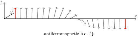
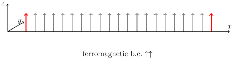
Figure 1: Sketch of the two boundary conditions considered in the manuscript with the corresponding minimum-energy profile $\vec{n}(x)$. For $\uparrow\uparrow$ b.c. we chose $\vec{n}(x)=(0,0,1)$, while for $\uparrow\downarrow$ b.c. $\vec{n}(x)$ is given by Eq. (19) – with arbitrary $x_{0}$ and $\varphi_{0}$ – and corresponds to the infinite-chain profile.

We consider the following classical Heisenberg Hamiltonian:

$$\mathcal{H}=-\sum_{i=0}^{L}\left[J\vec{S}_{i}\cdot\vec{S}_{i+1}+D(S_{i}^{z})^{2}\right]-D(S_{L+1}^{z})^{2}$$ (1)

where $D$ represents the anisotropy energy and $J$ the exchange coupling. Each spin variable $\vec{S}_{i}$ is a three-component unit vector associated with the $i$–th site of the lattice. The two spins at opposite boundaries are forced to lie along the easy anisotropy axis either parallel ($\uparrow\uparrow$) or antiparallel ($\uparrow\downarrow$) to each other (see the sketch in Fig 1). By computing the partition function for these two different boundary conditions (b.c.) the free-energy increase associated with the creation of a DW from a uniform ground state can be deduced. In this paper we will focus on broad DWs Billoni_11 , obtained for $J$ significantly larger than $D$, so that the micromagnetic limit for Hamiltonian (1) is meaningful:

$$\mathcal{H}=\int\limits_{0}^{L+1}\mathrm{d}x\,\left[\frac{J}{2}|\partial_{x}\vec{S}|^{2}-D\left(S^{z}(x)\right)^{2}\right]+\mathrm{const}\,,$$ (2)

(unitary lattice constant is assumed). Ferromagnetic b.c. ($\uparrow\uparrow$) are obtained setting $\vec{S}(x=0)=\vec{S}(x=L+1)=(0,0,1)$, while antiferromagnetic b.c. ($\uparrow\downarrow$) correspond to $\vec{S}(x=0)=(0,0,1)$ and $\vec{S}(x=L+1)=(0,0,-1)$. Following the procedure presented in Refs. Polyakov ; Politi_EPL_94 ; Billoni_11 , $\vec{S}(x)$ is decomposed in two vector fields

$$\vec{S}(x)=\vec{n}(x)\sqrt{1-\vec{\phi}^{2}}+\vec{\phi}(x)\,,$$ (3)

$\vec{\phi}(x)$ representing fluctuations and $\vec{n}(x)$ assumed to vary smoothly in space. If $|\vec{S}(x)|=1$ and $|\vec{n}(x)|=1$ are required, $\vec{n}(x)\cdot\vec{\phi}(x)=0$. Therefore, $\vec{\phi}(x)$ can be expressed on a local, two-dimensional basis orthogonal to $\vec{n}(x)$

$$\vec{\phi}(x)=\sum_{a}\phi_{a}\vec{e}_{a}\,,\qquad\mathrm{with}\quad|\vec{e}_{a}(x)|=1.$$ (4)

Through the decomposition given in Eq. (3), the Hamiltonian (2) can be expanded for small $\phi_{a}(x)$ up to quadratic terms, which makes it split in two contributions: $\mathcal{H}=\mathcal{H}[\vec{n}]+\mathcal{H}[\vec{\phi}]+\mathrm{const}$. $\mathcal{H}[\vec{n}]$ has the same form as Hamiltonian (2) provided that $\vec{S}(x)$ is substituted with $\vec{n}(x)$. The fluctuation Hamiltonian reads

$$\mathcal{H}[\vec{\phi}]=\sum_{a}\int\limits_{0}^{L+1}\mathrm{d}x\,\phi_{a}(x)\hat{H}_{a}\phi_{a}(x)\,,$$ (5)

in which $\hat{H}_{a}$ acts as a Schrödinger–like operator that takes a different form depending on the chosen slow-varying profile $\vec{n}(x)$. After having solved the eigenvalue problem

$$\hat{H}_{a}\psi(x)=\varepsilon\psi(x)\,,$$ (6)

each component (labeled by $a$) of the fluctuating field can be expanded on eigenfunctions of $\hat{H}_{a}$:

$$\phi_{a}(x)=\sum_{\nu}a_{a,\nu}\Psi_{a,\nu}(x)+\sum_{q}a_{a,q}\Phi_{a,q}(x)\,.$$ (7)

In our notation we associate the Greek index $\nu$ with (possible) bound states and $q$ with free states. By free states we mean functions which are delocalized throughout the spin chain, also when $L<\infty$. As a consequence of the finite size and of our choice of boundary conditions, such “free” states actually correspond to the wave functions of a free particle in a box when $\vec{n}(x)$ is assumed uniform (lower sketch in Fig. 1). In our vocabulary, there is no bound state in this case. When $\uparrow\downarrow$ b.c. are assumed, instead, Eq. (6) admits one bound state per component $a$. As it takes just one value, the label $\nu$ will be dropped henceforth from eigenfunctions $\Psi_{a,\nu}(x)$, coefficients $a_{a,\nu}$ and eigenvalues $\varepsilon_{a,\nu}$ (quantities associated with free states will still be denoted by the label $q$). If $\Psi_{a}(x)$ and $\Phi_{a,q}(x)$ are normalized properly, the expansion (7) allows rewriting the fluctuation Hamiltonian as

$$\mathcal{H}[\vec{\phi}]=\sum_{a}\left[\varepsilon_{a}|a_{a}|^{2}+\sum_{q}\varepsilon_{a,q}|a_{a,q}|^{2}\right]\,,$$ (8)

where $\varepsilon_{a}$ and $\varepsilon_{a,q}$ are the bound-state and free-state eigenvalues of Eq. (6), respectively.
A partition function that depends parametrically on the slow-varying field $\vec{n}(x)$ is obtained integrating over fluctuations, namely

$$\mathcal{Z}[\vec{n}]={\rm e}^{-\beta\mathcal{H}\left[\vec{n}\right]}\int\mathcal{D}[\vec{\phi}]\,\,{\rm e}^{-\beta\mathcal{H}\left[\vec{\phi}\right]}\,,$$ (9)

where $\int\mathcal{D}[\phi]$ stands for functional integral and $\beta=1/T$ ($k_{B}=1$ henceforth). This partition function can be rewritten as product of Gaussian integrals by making use of Eqs. (7) and (8):

$$\begin{split}\mathcal{Z}&[\vec{n}]={\rm e}^{-\beta\mathcal{H}\left[\vec{n}\right]}\times\left[\int{\underset{a}{\Pi}}\mathrm{d}a_{a}{\rm e}^{-\beta\varepsilon_{a}|a_{a}|^{2}}\right]^{n_{\rm dw}}\\ &\times\int{\underset{a,q}{\Pi}}\mathrm{d}a_{a,q}{\rm e}^{-\beta\varepsilon_{a,q}|a_{a,q}|^{2}}\,.\end{split}$$ (10)

For antiparallel b.c. ($\uparrow\downarrow$) $n_{\rm dw}=1$, meaning that one DW is present in the spin chain; while $n_{\rm dw}=0$ for parallel b.c. ($\uparrow\uparrow$). All the free states have positive energy, which makes their Gaussian integrals convergent. After this integration, Eq. (10) reads

$$\begin{split}\mathcal{Z}&[\vec{n}]={\rm e}^{-\beta\mathcal{H}\left[\vec{n}\right]}\times\left[\int{\underset{a}{\Pi}}\mathrm{d}a_{a}{\rm e}^{-\beta\varepsilon_{a}|a_{a}|^{2}}\right]^{n_{\rm dw}}\\ &\times\exp\left[-\frac{1}{2}\sum_{a,q}\log\left(\frac{\beta\varepsilon_{a,q}}{\pi}\right)\right]\,.\end{split}$$ (11)

The integration over bound-state amplitudes $\mathrm{d}a_{a}$ needs more care. We will see that bound states are associated with vanishing energy so that their contribution to the partition function cannot be evaluated through a standard Gaussian integration. The remedy to handle this divergence is presented in details in Ref. Leung_82, . As the explicit form of the bound-state eigenfunctions $\Psi_{a}(x)$ is required, we prefer to postpone this discussion. Further on, we will approximate the summation over free states $\sum_{a,q}$ in Eq. (11) with an integral. This approximation requires the knowledge of the density of states Currie_PRB_80 , which also needs to be determined previously by solving the eigenvalue problem in Eq. (6). From $\mathcal{Z}[\vec{n}]$ the free energy corresponding the to the b.c. $\uparrow\uparrow$ and $\uparrow\downarrow$ sketched in Fig. 1 can be computed. We will focus on the difference between those free energies $\Delta F=F_{\uparrow\downarrow}-F_{\uparrow\uparrow}=-T\log\left(Z_{\uparrow\downarrow}/Z_{\uparrow\uparrow}\right)$, which we identify with one DW free energy. Generally, choosing $\uparrow\uparrow$ boundary condition does not warrant the absence of DWs at finite temperatures. However, since we work with a finite system, we expect that DWs start forming spontaneously only when $\Delta F\lesssim 0$. So we can reasonably think that $\Delta F$ is a good estimate for one DW free energy as long as it is positive.

II.1 Schrödinger-like eigenvalue problem

Using the decomposition in Eq. (3), the terms entering Hamiltonian (2) can be expanded to second order in $\phi_{a}(x)$, which gives

$$\begin{split}(\partial_{x}\vec{S}(x))^{2}&=(1-\vec{\phi}^{2})(\partial_{x}\vec{n}(x))^{2}+\sum_{a}(\partial_{x}\phi_{a})^{2}+\sum_{a}c_{a}^{2}\phi_{a}^{2}\\ (S^{z}(x))^{2}&=(n^{z}(x))^{2}(1-\vec{\phi}^{2})+\sum_{a}\phi_{a}^{2}(e_{a}^{z})^{2}\,.\end{split}$$ (12)

$c_{a}$ are the components of $\partial_{x}\vec{n}$ on the basis $\vec{e}_{a}$ (remember that $|\vec{n}(x)|=1$ so that $\partial_{x}\vec{n}\perp\vec{n}$). The fluctuation Hamiltonian reads

$$\begin{split}&\hat{H}_{a}=-\frac{J}{2}\partial_{x}^{2}+V_{a}(x)\,,\qquad\mathrm{with}\\ &V_{a}(x)=\frac{J}{2}\left[c_{a}^{2}-(\partial_{x}\vec{n})^{2}\right]+D\left[(n^{z})^{2}-(e_{a}^{z})^{2}\right]\,.\end{split}$$ (13)

With our choice of boundaries, one has the equivalence

$$\int\limits_{0}^{L+1}\mathrm{d}x\,(\partial_{x}\phi)^{2}=-\int\limits_{0}^{L+1}\mathrm{d}x\,\phi\,\partial_{x}^{2}\phi\,,$$ (14)

which yields the second derivative in Eq. (13). The “potential” $V_{a}(x)$ will be specified by the choice of profile $\vec{n}(x)$. The latter will be chosen as the minimal-energy profile consistent with ferromagnetic and antiferromagnetic b.c.. These two cases are discussed separately in the following.

II.1.1 Uniform profile

When ferromagnetic ($\uparrow\uparrow$) b.c. are chosen the ground state is given by a uniform profile. Thus, we set $\vec{n}(x)=(0,0,1)$ or, equivalently, $\vec{n}=\vec{e}_{z}$ and $\vec{e}_{a}$ given by the two vectors $\vec{e}_{x,y}$ ($a=x,y$ for this case). Accordingly, the potential $V_{a}(x)$ takes the form

$$V_{a}=D+\begin{cases}0&x\in(0,L+1)\\ \infty&\mathrm{else}\end{cases}$$ (15)

so that the eigenvalue problem is formally equivalent to that of a particle in a box whose normalized eigenfunctions are given by

$$\Phi_{a,q}(x)=\sqrt{\frac{2}{L+1}}\sin(qx)\,,\qquad\mathrm{with}\quad a=x,y$$ (16)

with $q=l\,\pi/(L+1)$, $l=1,2,3,\ldots$ and eigenvalues

$$\varepsilon_{a,q}=\frac{J}{2}q^{2}+D\,.$$ (17)

II.1.2 Domain-wall profile

In the case of antiferromagnetic ($\uparrow\downarrow$) b.c., $\vec{n}$ is chosen to be

$$\begin{cases}n^{x}(x)&=\cos\varphi_{0}\,{\rm sech}(c(x-x_{0}))\\ n^{y}(x)&=\sin\varphi_{0}\,{\rm sech}(c(x-x_{0}))\\ n^{z}(x)&=-\tanh(c(x-x_{0}))\,,\end{cases}$$ (18)

where $c=\sqrt{2D/J}$ is the inverse DW width. Rigorously, the spin profile in Eq. (18) minimizes the energy of an infinite chain with $\uparrow\downarrow$ b.c., but here we will use it to build the Schrödinger–like equation for a finite chain (see Appendix D for further details). As we set no anisotropy in the hard plane ($xy$), nor we consider magnetostatic interaction, DWs parameterized by different angles $\varphi_{0}$ have the same energy (e.g., Bloch and Néel DWs). One of the two vectors $\vec{e}_{a}$ is the tangent vector $\vec{e}_{x_{0}}$

$$\begin{cases}e_{x_{0}}^{x}(x)&=\cos\varphi_{0}\tanh(c(x-x_{0}))\\ e_{x_{0}}^{y}(x)&=\sin\varphi_{0}\tanh(c(x-x_{0}))\\ e_{x_{0}}^{z}(x)&={\rm sech}(c(x-x_{0}))\end{cases}$$ (19)

that is proportional to $\partial_{x}\vec{n}$:

$$\begin{split}\partial_{x}\vec{n}&=-c\,{\rm sech}(c(x-x_{0}))\,\vec{e}_{x_{0}}\,,\qquad\mathrm{with}\\ c_{x_{0}}&=-c\,{\rm sech}\,(c(x-x_{0}))\,.\end{split}$$ (20)

The other one can be found from the vector product of $\vec{e}_{x_{0}}$ and $\vec{n}$: $\vec{e}_{\varphi_{0}}=\vec{e}_{x_{0}}\times\vec{n}=\left(-\sin{\varphi_{0}}\,,\,\cos{\varphi_{0}}\,,\,0\right)$ (note that $c_{\varphi_{0}}=0$). For our choice of profile and b.c., this vector coincides with the DW chirality B_Braun_AdvPhys_2012 , that is

$$\frac{1}{\pi}\int\limits_{0}^{L+1}\vec{n}\times\partial_{x}\vec{n}\,{\rm d}x=-\vec{e}_{\varphi_{0}}\,.$$ (21)

The motivation for labeling the vectors $\vec{e}_{a}$ with $a=x_{0},\,\varphi_{0}$ will be clear at the end of this paragraph and – we believe – will facilitate reading what follows. The components of the fluctuation field $\vec{\phi}(x)$ on the basis vectors $\vec{e}_{x_{0}}$ and $\vec{e}_{\varphi_{0}}$ will be labeled accordingly: $\phi_{x_{0}}$ and $\phi_{\varphi_{0}}$. The spatial dependence of $\vec{n}(x)$ and $\vec{e}_{x_{0}}(x)$ propagates to the potentials entering the Schrödinger-like equation associated with the two independent components of $\vec{\phi}(x)$:

$$V_{x_{0}}(x)=V_{\varphi_{0}}(x)=D\left[2\tanh^{2}(c(x-x_{0}))-1\right]\,.$$ (22)

In the general case in which an intermediate anisotropy axis is present, which breaks the $\varphi_{0}$ degeneracy in the $xy$ plane, the potentials $V_{x_{0}}(x)$ and $V_{\varphi_{0}}(x)$ are different. When the potentials in Eq. (22) are inserted into the eigenvalue problem (6), one obtains an equation which is a special case of the more general one:

$$\begin{split}&\hat{H}_{m}\psi(x)=\tilde{\varepsilon}\psi(x)\,,\qquad\mathrm{with}\\ &\hat{H}_{m}=-\partial_{\eta}^{2}+m(m+1)\tanh^{2}\eta\,,\end{split}$$ (23)

where the change of variable $\eta=c(x-x_{0})$ has been performed, the energy $\tilde{\varepsilon}$ is adimensional in units of $D$ and $m\in\mathbb{N}$. In terms of the lowering and raising operators

$$\begin{cases}&\hat{a}_{m}=\partial_{\eta}+m\tanh\eta\\ &\hat{a}^{\dagger}_{m}=-\partial_{\eta}+m\tanh\eta\,,\end{cases}$$ (24)

one has $\hat{H}_{m}=\hat{a}^{\dagger}_{m}\hat{a}_{m}+m$. In Appendix A we recall a demonstration HB_Braun_PRB94 that if $|\psi\rangle_{m}$ is an eigenstate of $\hat{H}_{m}$ then $\hat{a}^{\dagger}_{m+1}|\psi\rangle_{m}$ is an eigenstate of $\hat{H}_{m+1}$. This property allows us to construct the eigenstates of $\hat{H}_{1}$ – which corresponds to case treated in this paragraph ($\uparrow\downarrow$) – from the knowledge of the eigenstates of $\hat{H}_{0}=-\partial_{\eta}^{2}$. Operatively, this means that we can obtain the solution to the eigenvalue problem associated with the potentials in Eq. (22) by applying the raising operator $\hat{a}^{\dagger}_{1}$ to the eigenfunctions of a free-particle in a box $\psi_{0}(q,x)=A\cos(qx)+B\sin(qx)$, $A$ and $B$ being constants to be specified by b.c.. Details of the calculations are reported in Appendix B. To proceed in the derivation of the DW free energy we only need to know the density of states $\rho(q)$ and the eigenvalues $\varepsilon_{a,q}$. The last few have the same dependence on $q$ as in Eq. (17) but the allowed values of $q$ are different, which eventually yields a different $\rho(q)$ with respect to the case of ferromagnetic ($\uparrow\uparrow$) b.c.. In addition to these free states, the Schrödinger-like Eq. (6) (with the potentials given in Eq. (22)) also admits one bound state Fogedby84JPCSSP ; HB_Braun_PRB94 ; Winter_61 ; Yan_11 :

$$\Psi_{a}(x)=\sqrt{\frac{c}{2}}\,{\rm sech}(c(x-x_{0}))$$ (25)

with eigenvalue $\varepsilon_{a}=0$ (remember that we drop the index $\nu$ because there is just one bound state per component $a=x_{0},\,\varphi_{0}$). When an intermediate-anisotropy term $-D_{x}(S_{i}^{x})^{2}$ is added to Hamiltonian (1), the energy of the bound state $\Psi_{\varphi_{0}}(x)$ becomes positive. This suggests that the vanishing of $\varepsilon_{\varphi_{0}}$ be related to the degeneracy of the profile in Eq. (18) with respect to the angle $\varphi_{0}$, when $D_{x}=0$. In fact, $\partial_{\varphi_{0}}\vec{n}={\rm sech}(c(x-x_{0}))\,\vec{e}_{\varphi_{0}}$, meaning that the vector $\vec{e}_{\varphi_{0}}$ indicates the direction along which the minimum-energy profile is deformed in response to a variation $\delta\varphi_{0}$. In other words, any rotation on the $xy$ plane of the chiral (vector) degree of freedom – defined in Eq. (21) – does not affect the DW energy if $D_{x}=0$; while only reflections of the chirality vector, $\varphi_{0}\rightarrow\varphi_{0}+\pi$, leave the energy unchanged when $D_{x}\neq 0$ (e.g., left- and right-handed Bolch DWs are degenerate). On the contrary, the energy $\varepsilon_{x_{0}}$ remains zero also when an intermediate-anisotropy axis exists ($D_{x}\neq 0$). This is related to the degeneracy HB_Braun_PRB94 ; Leung_82 with respect to $x_{0}$, as confirmed by the equivalence $\partial_{x_{0}}\vec{n}=c\,{\rm sech}(c(x-x_{0}))\,\vec{e}_{x_{0}}$, obtained from Eq. (20) with the substitution $x\leftrightarrow x_{0}$.

II.2 Domain-wall free energy

In the case in which $\vec{n}(x)$ represents a DW profile ($\uparrow\downarrow$ b.c.), the considerations exposed above furnish a recipe to replace the integration over the amplitudes $\mathrm{d}a_{x_{0}}$ and $\mathrm{d}a_{\varphi_{0}}$ by integrals over the DW center $x_{0}$ and the angle $\varphi_{0}$, respectively. This makes it possible to evaluate the contribution of bound states to the partition function (11). From the relations between $\vec{e}_{x_{0},\varphi_{0}}$, $\partial_{x_{0}}\vec{n}$ and $\partial_{\varphi_{0}}\vec{n}$ the required Jacobian can be deduced Fogedby84JPCSSP ; Leung_82

$$\begin{split}&|\partial_{x_{0}}\vec{n}|\,\mathrm{d}x_{0}=\Psi_{x_{0}}(x)\mathrm{d}a_{x_{0}}\\ &|\partial_{\varphi_{0}}\vec{n}|\,\mathrm{d}\varphi_{0}=\Psi_{\varphi_{0}}(x)\mathrm{d}a_{\varphi_{0}}\end{split}\quad\Rightarrow\quad\begin{split}&\mathrm{d}a_{x_{0}}=\mathrm{d}x_{0}\sqrt{2c}\\ &\mathrm{d}a_{\varphi_{0}}=\mathrm{d}\varphi_{0}\sqrt{2/c}\,.\end{split}$$ (26)

The integrals we are interested in reduce to

$$\int{\underset{a=x_{0},\varphi_{0}}{\Pi}}\mathrm{d}a_{a}=2\int\limits_{0}^{L}\mathrm{d}x_{0}\int\limits_{0}^{2\pi}\mathrm{d}\varphi_{0}=4\pi L\,,$$ (27)

where the fact that $\varepsilon_{x_{0}}=\varepsilon_{\varphi_{0}}=0$ has been used and the factor 2 comes from the Jacobian deduced in Eq. (LABEL:eq25). Strictly speaking, it would be more appropriate to let the integral over $\mathrm{d}x_{0}$ range from $1/(2c)$ to $L+1-1/(2c)$. But, since this numerical factors do not affect the results significantly, we prefer to keep analytic expressions as simple as possible.
When a uniform $\vec{n}(x)$ is assumed ($\uparrow\uparrow$ b.c.), the eigenvalue problem in Eq. (6) does not admit bound-state solutions, thus we can formally set the integral in Eq. (27) equal to one. We approximate the remaining summation on the free states in Eq. (11) with an integral:

$$\sum_{q}\rightarrow\frac{1}{2}\int\limits_{-\infty}^{\infty}\,\rho(q)\,\mathrm{d}q\,.$$ (28)

The density of states has the form $\rho(q)=\rho_{\uparrow\uparrow}-\gamma(q)$, with

$$\gamma(q)=\frac{2c\tanh(c(L+1)/2)}{\pi(c^{2}\tanh^{2}(c(L+1)/2)+q^{2})}$$ (29)

and $\rho_{\uparrow\uparrow}=(L+1)/\pi$. The density of states for these linear excitations superimposed to a DW profile $\vec{n}(x)$ is derived in Appendix B. As defined in Eq. (29), $\gamma(q)$ corresponds to placing one DW in the middle of the chain ($x_{0}=(L+1)/2$). The general formula would depend parametrically on the coordinate of the DW center (see Eq. (91)), which renders the calculation of the partition function unusefully complicated. Eventually, the accuracy of all these approximations will be checked comparing analytic and numerical results (details about the numerical method will be given in Section III). Within these assumptions, the partition functions for the two b.c. sketched in Fig. 1 read:

$$\begin{split}\mathcal{Z}_{\uparrow\uparrow}&=\exp\left[-\frac{1}{2}\int\limits_{-\infty}^{\infty}\,\log\left(\frac{\beta\varepsilon_{a,q}}{\pi}\right)\rho_{\uparrow\uparrow}\,\mathrm{d}q\right]\\ \mathcal{Z}_{\uparrow\downarrow}&=4\pi L\,\mathrm{e}^{-\beta\mathcal{E}_{\rm dw}}\\ &\times\exp\left[-\frac{1}{2}\int\limits_{-\infty}^{\infty}\,\log\left(\frac{\beta\varepsilon_{a,q}}{\pi}\right)\left(\rho_{\uparrow\uparrow}-\gamma(q)\right)\mathrm{d}q\right]\,,\end{split}$$ (30)

where $\mathcal{E}_{\rm dw}=2\sqrt{2JD}$ represents the DW energy with respect to the uniform ground state, while $\varepsilon_{a,q}=Jq^{2}/2+D$ consistently with Eqs. (84) and (16). Equations (30) are obtained from Eq. (11) by setting $n_{\rm dw}=0,1$ for $\uparrow\uparrow$ and $\uparrow\downarrow$ b.c., respectively. We are now in the position to give an expression for the DW free energy:

$$\begin{split}\Delta F&=-T\log\left(Z_{\uparrow\downarrow}/Z_{\uparrow\uparrow}\right)=\mathcal{E}_{\rm dw}-T\log(4\pi L)\\ &-\frac{T}{2}\int\limits_{-\infty}^{\infty}\,\log\left(\frac{\beta J}{2\pi}(q^{2}+c^{2})\right)\gamma(q)\mathrm{d}q\,.\end{split}$$ (31)

Using the fact that

$$\int\limits_{-\infty}^{\infty}\,\frac{\log(q^{2}+c^{2})}{q^{2}+c_{L}^{2}}\mathrm{d}q=\frac{2\pi}{c_{L}}\log(c+c_{L})$$ (32)

with $c_{L}=c\tanh(c(L+1)/2)$, after some algebra, one obtains

$$\Delta F=\mathcal{E}_{\rm dw}-T\log\left[4\beta DL\left(1+\tanh(c(L+1)/2)\right)^{2}\right]\,.$$ (33)

Note that $\tanh(c(L+1)/2)$ approaches one in the limit $L\gg 1/c$.

II.3 Polyakov renormalization

When ferromagnetic b.c. are considered, the expansion in Eq. (7) involves only free states $\Phi_{a,q}(x)$, those given in Eq. (16). Thermal averages of the coefficients $a_{a,q}$ and their products are momenta of the Gaussian integrals entering the partition function $\mathcal{Z}[\vec{n}]$ and, therefore, fulfill the relations

$$\begin{split}&\langle a_{a,q}\rangle=0\\ &\langle a_{a,q}\,a_{a,q^{\prime}}\rangle=\frac{T}{2\,\varepsilon_{a,q}}\,\delta_{q,q^{\prime}}\end{split}$$ (34)

(equipartition theorem). From this it follows that thermal averages of the fluctuation-field components read

$$\begin{split}\langle\phi_{a}^{2}\rangle_{\uparrow\uparrow}&=\frac{T}{L+1}\sum_{q}\frac{\sin^{2}(qx)}{\varepsilon_{a,q}}\simeq\frac{T}{2(L+1)}\int\limits_{-\infty}^{\infty}\frac{\sin^{2}(qx)}{\varepsilon_{a,q}}\rho_{\uparrow\uparrow}\,\mathrm{d}q\\ &=\frac{T}{2\pi J}\int\limits_{-\infty}^{\infty}\frac{1-\cos(2qx)}{q^{2}+c^{2}}\mathrm{d}q\\ &=\frac{T}{\mathcal{E}_{\rm dw}}\left[1-\mathrm{e}^{-2cx}-\mathrm{e}^{-2c(L+1-x)}\right]\,;\end{split}$$ (35)

the first two terms of the last line come directly from integration on the complex plane, while the third one has been added by hand for symmetry with respect to the boundaries $x=0$ and $x=L+1$. This contribution is lost when the summation $\sum_{q}$ is approximated with an integral (first line).

Figure 2: (Color online). $\langle(S^{z}(x))^{2}\rangle$ obtained for $\uparrow\uparrow$ b.c.: Transfer-matrix calculation (symbols, T.M. in the legend) and analytic result (line) obtained combining Eq. (35) with Eq. (36): $\langle(S^{z}(x))^{2}\rangle=1-2\langle\phi_{a}^{2}\rangle_{\uparrow\uparrow}$. Calculation parameters: $D/J=0.01$, $T/J=0.02$, $L=100$ spins.

Starting from Eq. (12), it can be shown Billoni_11 ; Politi_EPL_94 that the following relations hold for thermal averages:

$$\begin{cases}\langle(\partial_{x}\vec{S})^{2}\rangle&=\left(1-\langle\phi_{a}^{2}\rangle_{\uparrow\uparrow}\right)\left(\partial_{x}\vec{n}\right)^{2}+\sum_{a}\langle\left(\partial_{x}\phi_{a}\right)^{2}\rangle_{\uparrow\uparrow}\\ \langle\left(S^{z}(x)\right)^{2}\rangle&=\left(1-3\langle\phi_{a}^{2}\rangle_{\uparrow\uparrow}\right)\left(n^{z}\right)^{2}+\langle\phi_{a}^{2}\rangle_{\uparrow\uparrow}\,.\end{cases}$$ (36)

In Fig. 2 we compare $\langle\left(S^{z}(x)\right)^{2}\rangle$ obtained by inserting the analytic formula for $\langle\phi_{a}^{2}\rangle_{\uparrow\uparrow}$ given in Eq. (35) with numerical results on a discrete lattice (see Section III for details). The Gaussian approximation agrees very well with numerics at low temperature. For an infinite system, the Gaussian approximation would give $\langle\phi_{a}^{2}\rangle_{\infty}=T/\mathcal{E}_{\rm dw}$, which is indeed recovered away from the boundaries (not shown). The more refined, Polyakov approach consists in integrating the free-state degrees of freedom progressively, starting from fluctuations associated with shorter spatial scales. Consistently with Eq. (36), this leads to renormalization of the spin-Hamiltonian parameters Polyakov ; Politi_EPL_94

$$\begin{cases}J\rightarrow&J\left(1-\langle\phi_{a}^{2}\rangle_{\mathrm{d}q}\right)\\ D\rightarrow&D\left(1-3\langle\phi_{a}^{2}\rangle_{\mathrm{d}q}\right)\end{cases}$$ (37)

with

$$\langle\phi_{a}^{2}\rangle_{\mathrm{d}q}=\frac{T}{2\pi J}\frac{1}{q^{2}+c^{2}}\mathrm{d}q\,.$$ (38)

The term $c^{2}$ at the denominator is usually neglected to facilitate the analytic treatment; the error due to this approximation will be compensated by a proper choice of cut-off at which the renormalization procedure stops.

Figure 3: (Color online). Domain-wall free energy $\Delta F$ as a function of temperature for different system sizes $L$ and $D/J=0.1$. Symbols (crosses $L=100$ and squares $L=20$) are numerical values obtained by means of transfer-matrix calculations (T.M. in the legend). Lines represent the prediction of Eq. (33), either using bare constants $D$ and $c$ or renormalized ones $D(\lambda_{\rm c})$ and $c(\lambda_{\rm c})$ (ren. in the legend), as described in the main text.

It is convenient to pass to the real space through the substitution $\lambda=1/q$ so that the renormalization flux takes the form

$$\begin{cases}&J(\lambda+\mathrm{d}\lambda)=J(\lambda)\left(1-\frac{T}{2\pi J(\lambda)}\mathrm{d}\lambda\right)\\ &D(\lambda+\mathrm{d}\lambda)=D(\lambda)\left(1-3\frac{T}{2\pi J(\lambda)}\mathrm{d}\lambda\right)\,.\end{cases}$$ (39)

The integration of the first differential equation is straightforward and gives $J(\lambda)=JZ(\lambda)$, with $Z(\lambda)=1-T\lambda/(2\pi J)$ and $J$ being the original, bare exchange constant appearing in Hamiltonian (1). Taking into account that $\mathrm{d}Z(\lambda)=-T\mathrm{d}\lambda/(2\pi J)$, the second equation takes the form

$$\frac{\mathrm{d}D(\lambda)}{D(\lambda)}=3\frac{\mathrm{d}Z(\lambda)}{Z(\lambda)}\quad\Rightarrow\quad D(\lambda)=DZ^{3}(\lambda)\,,$$ (40)

where, again, $D$ is the original, bare anisotropy constant and $D(\lambda)$ the renormalized one. The cut-off $\lambda_{\rm c}$ at which the renormalization stops can be chosen in order that the Gaussian result – consistent with $\langle\phi_{a}^{2}\rangle_{\infty}=T/\mathcal{E}_{\rm dw}$ – is recovered at low temperature, namely $\lambda_{\rm c}=2\pi J/\mathcal{E}_{\rm dw}=\pi/c$. The whole renormalization is meaningful as long as $Z(\lambda_{\rm c})>0$, that is for $T<\mathcal{E}_{\rm dw}$. This is not a problem because the requirement that the DW free energy be positive, $\Delta F\gtrsim 0$, is generally more strict.
In Fig. 3, the free-energy difference $\Delta F$ computed numerically with the transfer-matrix technique (see Section III) is compared with theoretical predictions. Two possible system sizes were considered $L=20,\,100$. The theoretical curve given in Eq. (33) and numerical points literally overlap at low temperature. At intermediate temperatures it turns out that a better agreement is achieved when $D$ is replaced by $D(\lambda_{\rm c})$ and $c$ by $c(\lambda_{\rm c})=c\,Z(\lambda_{\rm c})$ only in the argument of the logarithm. By increasing $L$, the temperature at which $\Delta F\simeq 0$ systematically lowers, as expected from the logarithmic dependence on $L$ in Eq. (33). For this reason the renormalization effects are less severe and already the Gaussian approximation works very well for $L=100$. However, for $L=20$ the prediction of Eq. (33) with bare constants (labeled with “Eq. (33)” the figure legend) deviates more significantly from the exact numerical results. In particular, the transfer-matrix calculation displays a concavity not shown by the theoretical curve obtained with bare values of $c$ and $D$. The concavity is, instead, reproduced at intermediate temperatures by Eq. (33) if renormalized constants $D(\lambda_{\rm c})$ and $c(\lambda_{\rm c})$ are used (labeled with “Eq. (33) ren.” in the figure legend).

II.4 Susceptibility and correlation length

In an infinite spin chain pair-spin correlations decay with the distance as $\langle S^{\alpha}(x+r)S^{\alpha}(x)\rangle=\langle\left(S^{\alpha}(x)\right)^{2}\rangle\,\mathrm{e}^{-|r|/\xi}$, where $\xi$ is the correlation length and $\alpha=x,y,z$. Henceforth, we will focus on their $z$ component and on the magnetic susceptibility along the easy axis, to which they are related through the equation

$$\begin{split}\chi&=-\frac{1}{L}\frac{\partial^{2}F}{\partial B_{z}^{2}}=\frac{(g\mu_{\rm B})^{2}}{T}\langle\left(S^{z}(x)\right)^{2}\rangle\sum_{r=-\infty}^{+\infty}\mathrm{e}^{-|r|/\xi}\\ &=\frac{(g\mu_{\rm B})^{2}}{T}\langle\left(S^{z}(x)\right)^{2}\rangle\coth\left(\frac{1}{2\xi}\right)\end{split}$$ (41)

with $\mu_{\rm B}$ Bohr magneton and $g$ Landé factor ($k_{B}=1$). In the high-temperature limit $\xi$ vanishes and $\langle\left(S^{\alpha}(x)\right)^{2}\rangle$ becomes independent of $\alpha=x,y,z$ so that the Curie law is recovered (with the substitution $\langle\left(S^{z}(x)\right)^{2}\rangle\rightarrow S(S+1)/3$). In the low-temperature limit $\langle\left(S^{z}(x)\right)^{2}\rangle\rightarrow S^{2}$, $\xi\gg 1$ and $\chi\,T\sim\xi$. The last relation is normally employed to extract information about the spin-Hamiltonian parameters directly from experimental susceptibility data. For the Ising chain $\xi\sim\mathrm{e}^{\beta\mathcal{E}_{\rm dw}}$ throughout a wide range of temperatures. Therefore, it is generally believed that the thermodynamics of anisotropic spin chains may be described with the Ising model just fitting the exchange interaction to the barrier that controls the exponential divergence of $\chi\,T$ ($\Delta_{\xi}$ in the literature). In a previous work Billoni_11 we showed that this is not appropriate for the model described by Hamiltonian (1) when DWs extend over several lattice units. This is the regime we address in the present work (the use of Hamiltonian (2) is legitimate only in this limit, $c\ll 1$). Existing expansions of $\xi$ often disagree among them and their applicability is limited to some undefined low-temperature region. Here we would like to give an analytic expression for $\xi$, based on the interplay between DWs and spin waves, and check it against numerics to establish its actual range of validity.
Figure 3 indicates that Eq. (33) combined with Polyakov renormalization provides a reasonable estimate for the DW free energy in a finite system. Among other applications, this formula can be used to evaluate the behavior of the correlation length $\xi$ as a function of temperature. Let us fix the temperature and define $\bar{L}$ as the critical length of the spin chain for which $\Delta F=0$. Apart from prefactors, the correlation length is expected to depend on temperature and on the spin-Hamiltonian parameters in the same way as $\bar{L}$.

Figure 4: (Color online). Correlation length in units of DW width, $c\,\xi$, computed for $D/J=0.1$. Symbols are obtained with the transfer-matrix algorithm for an infinite chain (T.M. in the legend). Lines represent analytic expressions given in the literature, Eqs. (43)–(44), and obtained by us. The dash-dotted (light-blue) curve (Eq. (46) in the legend) is obtained by continuing Eq. (45) with Eq. (46) for $\mathcal{E}_{\rm dw}/T<4.262$. The different theoretical curves have been rescaled by constant factors to match the numerical points at low temperatures.

It is convenient to express $\bar{L}$ in units of DW width. The implicit equation can be solved with the fixed-point method (see Appendix C for details). However, it turns out that the first iteration is accurate within 1.4% for any $D/J>0.1$. We will, thus, reasonably assume

$$c\bar{L}=\frac{\mathrm{e}^{\beta\mathcal{E}_{\rm dw}}}{4\beta\mathcal{E}_{\rm dw}Z(\lambda_{\rm c})}$$ (42)

as the solution. Note that the right-hand side of this equation only depends on $\beta\mathcal{E}_{\rm dw}$. In Ref. Billoni_11, it was shown that the correlation length in units of DW width is a universal function of the same variable. As anticipated, we expect the product $c\,\xi$ to scale like $c\bar{L}$. In Fig. 4, numerical results obtained with the transfer-matrix technique are compared with the prediction of Eq. (42) and other two expansions reported in the literature. More specifically, in Ref. Nakamura_77, ; Nakamura_78, it was proposed

$$\xi\sim\frac{1}{c}\,\mathrm{e}^{\beta\mathcal{E}_{\rm dw}}\,,$$ (43)

which differs by a temperature-dependent prefactor from the result obtained in Ref. Fogedby84JPCSSP, :

$$\xi\sim\frac{1}{c\,\beta\mathcal{E}_{\rm dw}}\,\mathrm{e}^{\beta\mathcal{E}_{\rm dw}}\,.$$ (44)

In Fig. 4, all analytic results have been rescaled by a constant in order to overlap the numerical points at low temperature. Equation (42) needs to be divided by a factor very close to the Euler constant. Our phenomenological treatment is summarized in the low-temperature expansion

$$\xi\simeq\frac{1}{4\,\mathrm{e}\,c\,\beta\mathcal{E}_{\rm dw}}\frac{\mathrm{e}^{\beta\mathcal{E}_{\rm dw}}}{Z(\lambda_{\rm c})}\,,$$ (45)

which corresponds to the short-dashed (blue) curve in Fig. 4. Compared with the other two low-temperature expansions, Eq. (45) reproduces the numerical points up to higher temperatures, but it fails as well for $T>\mathcal{E}_{\rm dw}/4$. More dramatic is the divergence of Eq. (45) as $T$ approaches $\mathcal{E}_{\rm dw}$, associated with the vanishing of $Z(\lambda_{\rm c})$. We understand this spurious effect as due to the fact that the cut-off $\lambda_{\rm c}$ at which renormalization stops becomes of the order of the system size, $\bar{L}$. Tentatively, we tried to tune this artifact by assuming that the contributions arising from spin waves (including Polyakov renormalization) somehow freeze when $\lambda_{\rm c}$ becomes of the order of the actual number of spins aligned along the same direction: $\bar{L}/2-3/2c$. This number is evaluated placing, ideally, the DW in the middle of a segment of length $\bar{L}$; the contribution of $1/c$ misaligned spins lying roughly on half DW is subtracted as well as that of $1/(2c)$ “blocked” spins at one boundary (consistently with Eq. (35)). One finds that $\lambda_{\rm c}=\bar{L}/2-3/2c$ when $\beta\mathcal{E}_{\rm dw}=4.262$. For higher temperatures, these considerations suggest to replace Eq. (45) by

$$\xi=\frac{A_{0}}{c}\,\mathrm{e}^{b\beta\mathcal{E}_{\rm dw}}\,,$$ (46)

with constants $A_{0}=0.3282$ and $b=0.5496$ determined by requiring the continuity of $\xi$ and its derivative with respect to $\beta\mathcal{E}_{\rm dw}$. The phenomenological curve obtained using Eq. (45) for $\beta\mathcal{E}_{\rm dw}>4.262$ and Eq. (46) otherwise is plotted with a dash-dotted (light-blue) line in Fig. 4. Though it is not fully justified on rigorous footing, this curve reproduces well the universal behavior of $c\,\xi$ versus $\beta\mathcal{E}_{\rm dw}$ till the correlation length becomes of the order of the DW width ($c\,\xi\simeq 1$). At such short scales the notion of correlation length itself becomes somewhat meaningless. A compact, analytic expression for the correlation length is provided by Eq. (110) in Appendix C.

Nowadays, the magnetic susceptibility of the model considered here can be obtained numerically essentially with negligible computational effort. However, the search for an accurate expansion of $\xi$ has attracted a remarkable interest in the community of Single-Chain Magnets. It should be kept in mind that in real systems defects and impurities limit the chain size to $10^{2}-10^{4}$ consecutive, interacting spins. For typical values of $J$ and $D$ one has $c\simeq 0.1$. Therefore, the behavior of the correlation length can be studied experimentally only for $T>\mathcal{E}_{\rm dw}/6$, for the purest spin chains, or $T>\mathcal{E}_{\rm dw}/4$, in worst cases. When the latter scenario occurs, Eq. (46) suggests that the barrier $\Delta_{\xi}$, defined as $\xi\sim\mathrm{e}^{\beta\Delta_{\xi}}$, should approach half of the DW energy $\mathcal{E}_{\rm dw}$. Indeed, this has been observed in Mn(III)-TCNE molecular spin chains Ishikawa_12 ; Balanda_06 , whose main thermodynamic features should be captured by the model Hamiltonian (1). In a recently published review article Zhang_RSC_2013 it was pointed out that Eq. (43) does not succeed in reproducing the measured susceptibility of this family of spin chains (though Eq. (43) was implicitly attributed to Ref. Billoni_11, instead of Ref. Nakamura_78, ).

The temperature dependence of $\langle\left(S^{z}(x)\right)^{2}\rangle$ can also affect the magnetic susceptibility at intermediate temperatures, $T>\mathcal{E}_{\rm dw}/4$ (see Eq. (41)). According to Eq. (36) and following ones, also this quantity should depend – to a large extent – only on $\beta\mathcal{E}_{\rm dw}$. In passing, we note that within our classical model the correct Curie constant cannot be recovered at high temperature: a fully quantum-mechanical calculation would be needed. Though worth mentioning, this question lies beyond the scope of the present work.

III Numerical checks

In this Section we describe and critically comment the numerical calculations that were made in order to check robustness and limitations of our analytic results.

The derivation of Eq. (33) strongly relies on the solution to Eq. (6) and on the correctness of the density of states $\rho(q)$ given in Eq (29). All these intermediate passages were checked diagonalizing the equivalent discrete-lattice problem, as explained in details in Appendix B.

The transfer-matrix algorithm and how finite size constrains the minimal-energy spin profile will be discussed in separate subsections.

III.1 Finite-size transfer matrix

The thermodynamic properties of the model described by Hamiltonian (1) and – more generally – of any classical-spin chain with nearest-neighbor interactions can be computed with the transfer-matrix technique. This approach has been largely used to derive analytic Nakamura_77 ; Nakamura_78 ; Scalapino_75 and numerical results Blume75PRB ; Tannous for infinite chains. Less frequently it has been employed to study finite systems Vindigni06APA , for which more flexible methods, e.g. Metropolis Monte-Carlo, exist. However, for our specific problem of computing the free-energy difference between the configurations sketched in Fig. 1, the transfer-matrix approach turned out to be extremely efficient. Let us separate the bulk interactions from those characterizing the spins at boundaries

$$\mathcal{H}=-\sum^{L-1}_{i=1}V_{\rm bulk}(\vec{S}_{i},\,\vec{S}_{i+1})-V_{\rm bc}(\vec{S}_{1})-V_{\rm bc}(\vec{S}_{L})\,.$$ (47)

Defining

$$\begin{split}&V_{\rm exch}(\vec{S}_{i},\,\vec{S}_{i+1})=J\vec{S}_{i}\cdot\vec{S}_{i+1}\\ &V_{\rm ss}(\vec{S}_{i})=D\left(S^{z}_{i}\right)^{2}\end{split}$$ (48)

we have

$$\begin{split}&V_{\rm bulk}(\vec{S}_{i},\,\vec{S}_{i+1})=V_{\rm exch}(\vec{S}_{i},\,\vec{S}_{i+1})\\ &\qquad+\frac{1}{2}\left(V_{\rm ss}(\vec{S}_{i})+V_{\rm ss}(\vec{S}_{i+1})\right)\\ &V_{\rm bc}(\vec{S}_{1})=\frac{1}{2}V_{\rm ss}(\vec{S}_{1})+J{S}^{z}_{1}\\ &V_{\rm bc}(\vec{S}_{L})=\frac{1}{2}V_{\rm ss}(\vec{S}_{L})\pm J{S}^{z}_{L}\,,\end{split}$$ (49)

the last term being plus for $\uparrow\uparrow$ b.c. and minus for $\uparrow\downarrow$ b.c.. $V_{\rm exch}$ can possibly describe anisotropic exchange, Dzyaloshinskii-Moriya interaction, etc., and $V_{\rm ss}$ any type of single-spin interaction (other anisotropy terms, Zeeman energy, etc.). With these conventions, the transfer-matrix kernel Wyld takes the form

$$\mathcal{K}_{\rm TM}(\vec{S}_{i},\,\vec{S}_{i+1})=\exp\left[\beta V_{\rm bulk}(\vec{S}_{i},\,\vec{S}_{i+1})\right]\,.$$ (50)

The latter defines the following eigenvalue problem:

$$\int\mathcal{K}_{\rm TM}(\vec{S}_{i},\,\vec{S}_{i+1})W_{m}(\vec{S}_{i+1})d\Omega_{i+1}=\lambda_{m}W_{m}(\vec{S}_{i})$$ (51)

whose eigenvalues may typically be ordered from the largest to the smallest one:

$$\lambda_{0}>\lambda_{1}>\lambda_{2}>\ldots$$

The eigenvalue problem (51) can be solved analytically only in few fortunate cases Fisher . Generally, it can be converted into a linear-algebra problem and solved numerically by discretizing the unitary sphere Stroud ; McLaren ; Abramowitz . For each temperature, the number of points used to sample the solid angle was increased until the desired precision in the free-energy calculation was reached. Once that eigenvalues and eigenvectors are known, the partition function is given by

$$\begin{split}&\mathcal{Z}_{\rm TM}=\sum_{m}\lambda_{m}^{L-1}w_{m}^{1}w_{m}^{L}\,\,\,\,\,\,\,\,\,\,\,\,\,\,\,\,\,\text{with}\\ &w_{m}^{1}=\int\exp\left[\frac{1}{2}\beta V_{\rm bc}(\vec{S}_{1})\right]W_{m}(\vec{S}_{1})d\Omega_{1}\\ &w_{m}^{L}=\int\exp\left[\frac{1}{2}\beta V_{\rm bc}(\vec{S}_{L})\right]W_{m}(\vec{S}_{L})d\Omega_{L}\,.\end{split}$$ (52)

The calculation of $Z_{\uparrow\downarrow}$ and $Z_{\uparrow\uparrow}$ just requires to change one sign in the definition of $V_{\rm bc}(\vec{S}_{L})$ given in Eq. (LABEL:TM_V_FS). In this way $\Delta F=-T\log\left(Z_{\uparrow\downarrow}/Z_{\uparrow\uparrow}\right)$ was computed also numerically to check the validity of Eq. (33). Results are plotted in Fig. 3. Further details concerning the calculation of $\langle(S^{z}(x))^{2}\rangle$ shown in Fig. 2 may be found in Ref. Vindigni06APA, , while details about how to compute the correlation length for the infinite chain (Fig. 4) are given in Ref. Billoni_11, .

III.2 General spin profile

The whole theoretical treatment developed in the previous and in the next Sections strongly depends on the profile $\vec{n}(x)$ assumed in Eq. (18). Strictly speaking, this profile minimizes the DW energy of an infinite chain when the micromagnetic limit is legitimate (i.e., for $c\ll 1$). Still working with broad DWs, analytic expressions can be derived for the case of $L<\infty$, which are recalled for the reader’s convenience in Appendix D. The accuracy of those analytic results was – in turn – checked against a discrete-lattice calculation based on non-linear maps trallori:94 ; rettori:95 ; trallori:96 . The most remarkable fact is that when the DW width becomes of the order of the system size ($L$) the dependence of $n^{z}(x)$ on the spatial coordinate crosses over from hyperbolic tangent to cosine (see Fig. 7). This imposes a natural range of validity to our model, which depends on the size of the characteristic length involved in a specific calculation. For the correlation length, e.g., meaningful analytic results can be derived only as long as $\xi\gtrsim 1/c$. We already commented on this while deriving Eq. (46). In the next Section we will discuss the temperature dependence of the period of modulation of 2d striped domain patterns. Also in this case, our considerations are expected to hold as long as the separation between two successive DWs is much larger than $1/c$. Since the period of modulation is found to decrease with increasing temperature, this self-consistency requirement eventually sets a high-temperature threshold above which our theory cannot be applied. Remarkably, the mean-field approach prescribes the low-temperature stripe phase to evolve into a single-cosine modulation at the mean-field Curie temperature Ale_PRB_08 ; Pighin_PRE_12 . However, since the mean-field approximation is known to overestimate the Curie temperature, in realistic systems it may happen that long-range magnetic order is lost before single-cosine modulation is attained. Summarizing, if for some reason the period of modulation is constrained to be of the order of $1/c$, a single-cosine modulation is expected. Whether this is necessarily the case when the true Curie temperature of a magnetic film is approached remains – to the best of our knowledge – not clear.

IV Domain walls in thin films

The same treatment presented up to now can be extended to DWs described by the spin profile in Eq. (18) embedded in 2d or 3d magnetic lattices. Here we focus on 2d systems, realized in thin ferromagnetic films or (flat) nanowires. More concretely, we address systems whose thickness, $\tau$, (defined along the $z$ direction) is smaller than the DW width: $\tau<1/c$. The generalization of Hamiltonian (2) to two dimensions reads

$$\mathcal{H}=\int\limits_{0}^{L_{y}+1}\mathrm{d}y\int\limits_{0}^{L_{x}+1}\left[\frac{J}{2}|\nabla\vec{S}|^{2}-D\left(S^{z}\right)^{2}\right]\mathrm{d}x\,,$$ (53)

where $L_{x}$ and $L_{y}$ denote the lateral extensions – in lattice units – of the system along $x$ and $y$ direction, respectively. Exchange and anisotropy constants are related to the atomic counterparts by the thickness: $J=\tau J_{\rm atom}$ and $D=\tau D_{\rm atom}$ ($\tau$ being the number of monolayers in the film). The vector field defining the local spin direction is a function of two spatial variables $\vec{S}=\vec{S}(x,y)$, but it can still be decomposed as in Eq. (3). The major difference is that the fluctuation field becomes a function of $x$ and $y$, $\vec{\phi}(x,y)$, while $\vec{n}(x)$ is assumed to depend only on $x$. Strictly speaking, the assumption of a DW profile being described by Eq. (18) does not allow considering complex magnetic-domain patterns, such as bubbles or labyrinths. Those patterns are not really the focus of the present paper, which rather deals with thermal properties of DWs. Being fully determined by $\vec{n}(x)$, the same basis set $\vec{e}_{a}$ defined for the 1d case can be employed to study Gaussian fluctuations about a DW hosted in a 2d lattice. Generally, the corresponding Schrödinger–like operator is obtained by adding a free-particle term, acting along the $y$ direction, to the operators $\hat{H}_{a}$ defined previously:

$$\hat{H}_{a}^{\rm 2d}=-\frac{J}{2}\partial_{y}^{2}+\hat{H}_{a}\,.$$ (54)

For the uniform case, $\vec{n}=\vec{e}_{z}$, the eigenfunctions of $\hat{H}_{a}^{\rm 2d}$ are the same as those of a free particle in a box:

$$\Phi_{a,q_{x},q_{y}}(x,y)=\frac{2\,\sin(q_{x}x)\sin(q_{y}y)}{\sqrt{(L_{x}+1)(L_{y}+1)}}\,,$$ (55)

with $q_{\alpha}=l_{\alpha}\,\pi/(L_{\alpha}+1)$, $l_{\alpha}=1,2,3,\ldots$ ($\alpha=x,y$) and eigenvalues

$$\varepsilon_{a,q_{x},q_{y}}=\frac{J}{2}\left(q_{x}^{2}+q_{y}^{2}\right)+D\,.$$ (56)

When $\vec{n}(x)$ is chosen as in Eq. (18), the free-state eigenfunctions are given by

$$\Phi_{a,q_{x},q_{y}}(x,y)=\sqrt{\frac{2}{L_{y}+1}}\sin(q_{y}y)\Phi_{a,q_{x}}(x)\,,$$ (57)

with the same eigenvalues as in Eq. (56), $\Phi_{a,q_{x}}(x)$ being the eigenfunctions defined in Appendix B. The bound-state contribution reads

$$\Psi_{a,q_{y}}(x,y)=\sqrt{\frac{2}{L_{y}+1}}\sin(q_{y}y)\Psi_{a}(x)\,,$$ (58)

with $\Psi_{a}(x)$ defined in Eq. (25) and eigenvalues $\varepsilon_{a,q_{y}}=Jq_{y}^{2}/2$ (for both components $a=x_{0},\varphi_{0}$). By analogy with the 1d case, each component of the fluctuating field $\vec{\phi}(x,y)$ can be expanded on eigenfunctions of the operator $\hat{H}_{a}^{\rm 2d}$ defined in Eq. (54). Finally, the fluctuation Hamiltonian can be written as

$$\mathcal{H}[\vec{\phi}]=\sum_{a}\left[\sum_{q_{y}}\varepsilon_{a,q_{y}}|b_{a,q_{y}}|^{2}+\sum_{q_{x},q_{y}}\varepsilon_{a,q_{x},q_{y}}|b_{a,q_{x},q_{y}}|^{2}\right],$$ (59)

where $b_{a,q_{y}}$ and $b_{a,q_{x},q_{y}}$ are the projections of a generic $\phi_{a}(x,y)$ on the basis functions $\Psi_{a,q_{y}}(x,y)$ and $\Phi_{a,q_{x},q_{y}}(x,y)$, respectively. Using the same conventions as in Eq. (11), the partition function is now given by

$$\begin{split}\mathcal{Z}&[\vec{n}]={\rm e}^{-\beta\mathcal{H}\left[\vec{n}\right]}\times\left[\int{\underset{a,q_{y}}{\Pi}}\mathrm{d}b_{a,q_{y}}{\rm e}^{-\beta\varepsilon_{a,q_{y}}|b_{a,q_{y}}|^{2}}\right]^{n_{\rm dw}}\\ &\times\exp\left[-\frac{1}{2}\sum_{a,q_{x},q_{y}}\log\left(\frac{\beta\varepsilon_{a,q_{x},q_{y}}}{\pi}\right)\right]\end{split}$$ (60)

(the label $\nu$ has been dropped because it takes just one value for each component $a$).

Let us consider first the contribution of the bound state associated with translation invariance of DW centers, $x_{0}$. We can formally use the substitution defined in Eq. (LABEL:eq25) and replace each amplitude variable by the corresponding coordinate of DW center $b_{x_{0},q_{y}}=x_{0}(q_{y})\sqrt{2c}$ so that

$$\begin{split}\mathcal{Z}_{x_{0}}&=\int{\underset{x_{0},q_{y}}{\Pi}}\mathrm{d}b_{x_{0},q_{y}}{\rm e}^{-\beta\varepsilon_{x_{0},q_{y}}|b_{x_{0},q_{y}}|^{2}}\\ &=(2c)^{L_{y}/2}\int{\underset{q_{y}}{\Pi}}\mathrm{d}x_{0}(q_{y})\exp{\left[-\frac{\beta\mathcal{E}_{\rm dw}}{2}q_{y}^{2}|x_{0}(q_{y})|^{2}\right]}\,,\end{split}$$ (61)

where the equivalence $\mathcal{E}_{\rm dw}=2Jc$ has been used. The dependence on $q_{y}$ in $x_{0}(q_{y})$ is better understood by thinking that in the ground state the DW develops as a straight line along $y$. Therefore, $x_{0}(q_{y})$ actually describes the displacement field associated with a corrugation of the DW induced by thermal fluctuations. In fact, a 1d Hamiltonian for elastic displacements (with “stiffness” $\mathcal{E}_{\rm dw}$)

$$\mathcal{H}_{\rm el}=\frac{\mathcal{E}_{\rm dw}}{2}\sum_{y}\left(x_{0}(y+1)-x_{0}(y)\right)^{2}$$ (62)

would yield a partition function equal to Eq. (61) for $q_{y}\sim 0$, namely in the continuum-limit formalism. However, if the lattice discreteness is reintroduced, undesired divergences are avoided. From textbooks it is known that Hamiltonian (62) reads

$$\mathcal{H}_{\rm el}=2\mathcal{E}_{\rm dw}\sum_{q_{y}}\sin^{2}\left(\frac{q_{y}}{2}\right)|x_{0}(q_{y})|^{2}$$ (63)

in the appropriate Fourier space with $q_{y}=l_{y}\,\pi/(L_{y}+1)$ and $1\leq l_{y}\leq L_{y}$. When the Boltzmann weights in Eq. (61) are replaced with $\beta\mathcal{H}_{\rm el}$, after Gaussian integrations with respect to $\mathrm{d}x_{0}$, one obtains

$$\mathcal{Z}_{x_{0}}=(2c)^{L_{y}/2}\exp{\left\{-\frac{1}{2}\sum_{q_{y}}\log\left[\frac{2\beta\mathcal{E}_{\rm dw}}{\pi}\sin^{2}\left(\frac{q_{y}}{2}\right)\right]\right\}}\,.$$ (64)

For $L_{y}\gg 1$, one has

$$\begin{split}\sum_{q_{y}}\log\left[\sin\left(\frac{q_{y}}{2}\right)\right]&\simeq\frac{L_{y}+1}{\pi}\int\limits^{\pi}_{0}\log\left[\sin\left(\frac{q_{y}}{2}\right)\right]{\rm d}q_{y}\\ &=-(L_{y}+1)\log 2\end{split}$$ (65)

which leads to

$$\mathcal{Z}_{x_{0}}=\left(\frac{2\pi}{\beta J}\right)^{L_{y}/2}\,.$$ (66)

(within the present approximation $L_{y}+1\simeq L_{y}$).

With a similar strategy, the contribution due to the bound state with vanishing energy associated with degeneracy in $\varphi_{0}$ can be evaluated. Still from Eq. (LABEL:eq25) it follows that $b_{\varphi_{0},q_{y}}=\varphi_{0}(q_{y})\sqrt{2/c}$. The corresponding factor in the partition function is transformed accordingly

$$\begin{split}\mathcal{Z}_{\varphi_{0}}&=\int{\underset{\varphi_{0},q_{y}}{\Pi}}\mathrm{d}b_{\varphi_{0},q_{y}}{\rm e}^{-\beta\varepsilon_{\varphi_{0},q_{y}}|b_{\varphi_{0},q_{y}}|^{2}}\\ &=\left(\frac{2}{c}\right)^{L_{y}/2}\int{\underset{q_{y}}{\Pi}}\mathrm{d}\varphi_{0}(q_{y})\exp{\left[-\frac{\beta J}{c}q_{y}^{2}|\varphi_{0}(q_{y})|^{2}\right]}\,.\end{split}$$ (67)

Establishing the same analogy as before, with a “stiffness” $2J/c$, a contribution equivalent to Eq. (66) is recovered, i.e. $\mathcal{Z}_{\varphi_{0}}=\mathcal{Z}_{x_{0}}$. On a more physical basis, the Boltzmann weight in Eq. (67) may be thought of as arising from an XY-model Hamiltonian

$$\begin{split}\mathcal{H}_{\rm xy}&=-\frac{2J}{c}\sum_{y}\cos\left[\varphi_{0}(y+1)-\varphi_{0}(y)\right]+\frac{2J}{c}L_{y}\\ &=-\frac{2J}{c}\sum_{y}\vec{e}_{\varphi_{0}}(y+1)\cdot\vec{e}_{\varphi_{0}}(y)+\frac{2J}{c}L_{y}\end{split}$$ (68)

involving the $\varphi_{0}$ angles of different arrays of spins, labeled by $y$. From the second line it is clear that $\mathcal{H}_{\rm xy}$ describes the effective coupling between chirality vectors of neighboring chains. Along this line, Eq. (67) can equivalently be written as

$$\begin{split}\mathcal{Z}_{\varphi_{0}}&\simeq\left(\sqrt{\frac{2}{c}}\,{\rm e}^{-2\beta J/c}\right)^{L_{y}}\int\limits_{-\pi}^{\pi}\mathrm{d}\varphi_{0}(1)\dots\mathrm{d}\varphi_{0}(L_{y})\\ &\exp{\left[\frac{2\beta J}{c}\sum_{y}\cos\left(\varphi_{0}(y+1)-\varphi_{0}(y)\right)\right]}\,.\end{split}$$ (69)

In terms of relative angles $\delta_{y}=\varphi_{0}(y+1)-\varphi_{0}(y)$ (and assuming $L_{y}+1\simeq L_{y}$) the above expression takes the form

$$\begin{split}\mathcal{Z}_{\varphi_{0}}&=\left(\sqrt{\frac{2}{c}}\,{\rm e}^{-2\beta J/c}\right)^{L_{y}}\left[\int\limits_{-\pi}^{\pi}\mathrm{d}\delta_{y}{\rm e}^{\frac{2\beta J}{c}\cos\left(\delta_{y}\right)}\right]^{L_{y}}\\ &=\left[2\pi\sqrt{\frac{2}{c}}\,{\rm e}^{-2\beta J/c}\,\mathcal{I}_{0}\left(\frac{2\beta J}{c}\right)\right]^{L_{y}}\end{split}$$ (70)

where $\mathcal{I}_{0}(\kappa)$ is the modified Bessel function of the first kind. For $2\beta J/c\gg 1$ (low temperatures) it is $\mathcal{I}_{0}(\kappa)\simeq\mathrm{e}^{\kappa}/\sqrt{2\pi\kappa}$ and $\mathcal{Z}_{\varphi_{0}}=\mathcal{Z}_{x_{0}}$ is recovered again.

As for 1d case, we focus on the ratio between the partition functions obtained for $\uparrow\downarrow$ and $\uparrow\uparrow$ b.c.. For one DW embedded in a thin film that is

$$\begin{split}&\frac{\mathcal{Z}_{\uparrow\downarrow}}{\mathcal{Z}_{\uparrow\uparrow}}=\mathrm{e}^{-\beta L_{y}\mathcal{E}_{\rm dw}}\mathcal{Z}_{x_{0}}\mathcal{Z}_{\varphi_{0}}\\ &\times\exp\left[\frac{1}{2}\sum_{q_{y}}\int\limits_{-\infty}^{\infty}\log\left(\frac{\beta J(q_{x}^{2}+q_{y}^{2}+c^{2})}{2\pi}\right)\gamma(q_{x})\,{\rm d}q_{x}\right].\end{split}$$ (71)

Note that only the summation over the $q_{x}$ label has been substituted with an integral (following the same conventions as in Eqs. (28) and (29)). Moreover, the fact that the energies $\varepsilon_{a,q_{x},q_{y}}$ in Eq. (56) actually do not depend on the label $a$ has been used. Exploiting again Eq. (32), the argument of the exponential in Eq. (71) can be approximated as

$$\begin{split}&\sum_{q_{y}}\left[\log\left(\frac{\beta J}{2\pi}\right)+2\log\left(c_{L}+\sqrt{q_{y}^{2}+c^{2}}\right)\right]\\ &\simeq L_{y}\log\left(\frac{\beta Jc_{L}^{2}}{2\pi}\right)\\ &+\frac{2(L_{y}+1)}{\pi}\int\limits_{0}^{\pi}\log\left[1+\sqrt{\left(\frac{q_{y}}{c_{L}}\right)^{2}+\left(\frac{c}{c_{L}}\right)^{2}}\right]\mathrm{d}q_{y}\end{split}$$ (72)

where we considered $L_{y}\gg 1$ and $c_{L}=c\tanh(c(L_{x}+1)/2)$ now. The integral in the last line of Eq. (LABEL:eq65) can be solved analytically

$$\begin{split}&\int\limits_{0}^{\pi}\dots\mathrm{d}q_{y}=\pi\,\left[\log\left(1+\tilde{c}\,\cosh t\right)\right]+c_{L}\,t-\pi\\ &-2c_{L}\sqrt{\tilde{c}^{2}-1}\,\arctan\left[\sqrt{\frac{\tilde{c}-1}{\tilde{c}+1}}\tanh\left(\frac{t}{2}\right)\right]\\ &{\overset{L_{x}\gg 1}{=}}\pi\,\log\left(1+\sqrt{1+\left(\frac{\pi}{c}\right)^{2}}\right)+c\,{\rm arcsinh}\left(\frac{\pi}{c}\right)-\pi\end{split}$$ (73)

with $\sinh t=\pi/c$ and $\tilde{c}=c/c_{L}$. The latter approaches one when $L_{x}\gg 1$ is considered. To the leading order, the free energy per unit length of a DW embedded in a thin film, whose linear dimensions are much larger than the lattice spacing, reads

$$\begin{split}\mathcal{F}_{\rm dw}&=-\frac{T}{L_{y}}\log\left(Z_{\uparrow\downarrow}/Z_{\uparrow\uparrow}\right)\\ &=\mathcal{E}_{\rm dw}-2\,T\left(\frac{c}{\pi}\,{\rm arcsinh}\left(\frac{\pi}{c}\right)-1\right)\\ &-2\,T\,\log\left[c\left(1+\sqrt{1+\left(\frac{\pi}{c}\right)^{2}}\right)\right]-\frac{T}{L_{y}}\log(4\pi L_{x})\end{split}$$ (74)

in which $\mathcal{Z}_{\varphi_{0}}=\mathcal{Z}_{x_{0}}$ has been assumed for the sake of simplicity. The last entropic term arises from two contributions neglected in $\mathcal{Z}_{x_{0}}$ and $\mathcal{Z}_{\varphi_{0}}$, namely a rigid translation of the DW as a whole and a rigid rotation of the chirality vectors. Those contributions have been already computed for the 1d case in Eq. (27), for which $y$ takes just one value. Even if this entropic term practically does not affect the free energy for $L_{x},L_{y}\gg 1$, it is important in relation to the underlying degeneracies with respect to $x_{0}$ and $\varphi_{0}$. In fact, these degeneracies eventually determine the i) floating of magnetic-domain patterns and ii) the vanishing of critical current for DW motion in nanowires with no intermediate anisotropy ($D_{x}=0$).

IV.1 Positional order of domain walls

The fact that both $\mathcal{Z}_{\varphi_{0}}$ and $\mathcal{Z}_{x_{0}}$ arise from elastic-like Hamiltonians has important implications which deserve some further comment. As already pointed out, $\mathcal{Z}_{x_{0}}$ is associated with corrugation of the DW as a function of $y$ (see the sketch in Fig. 5). In the ideal case considered here, this instability destroys positional order (defined by the profile $\vec{n}$) at finite temperatures. In real films positional order may be stabilized by some substrate anisotropy, pinning or dipolar interaction. The last one is responsible for the emergence of magnetic-domain patterns in films magnetized out of plane. In this context, Eq. (74) may be applied to study the temperature dependence of the optimal period of modulation for a stripe pattern, known to be the ground state Whitehead_PRB_95 ; Pighin_JMMM_10 ; Giuliani_PRB_07 ; Giuliani_PRB_11 (gray and white domains in Fig. 5). At zero temperature, a modulated phase results from the competition between magnetostatic energy (which favors in this case antiparallel alignment of spin pairs) and the energy cost to cerate DWs. Several approaches lead to the same scaling of the characteristic period of modulation Whitehead_PRB_95 ; Pighin_JMMM_10 ; Oliver_PRB_10 : $L_{\rm stripes}\sim{\rm e}^{\mathcal{E}_{\rm dw}/(4\Omega\tau^{2})}$, with $\Omega=\mu_{0}M_{\rm s}^{2}\mathfrak{a}^{3}/4\pi$ being the strength of dipolar interaction, $\tau$ the adimensional film thickness, $\mathfrak{a}$ the dimensional lattice constant and $M_{\rm s}$ the saturation magnetization. (remember that in this Section it is $\mathcal{E}_{\rm dw}=2\tau\sqrt{2J_{\rm atom}D_{\rm atom}}$). A first-order estimate of thermal effects is obtained by replacing $\mathcal{E}_{\rm dw}$ in the expression of $L_{\rm stripes}$ with $\mathcal{F}_{\rm dw}$ defined in Eq. (74): $L_{\rm stripes}\sim{\rm e}^{\mathcal{F}_{\rm dw}/(4\Omega\tau^{2})}$. The latter is consistent with a decrease of the period of modulation with increasing temperature, as observed in experiments Oliver_PRL_06 ; Niculin_PRL_10 and predicted by mean-field approach Ale_PRB_08 ; Oliver_PRB_10 . Note that in deducing the DW free energy $\mathcal{F}_{\rm dw}$ dipolar interaction was totally overlooked. For instance, this interaction is known to produce an effective intermediate anisotropy that stabilizes Bloch type of DWs in films magnetized out of plane. Strictly speaking, since we assumed $D_{x}=0$, our treatment should not apply to stripped patterns emerging in those films. A more accurate study of this specific phenomenon – which we intend to address in a forthcoming paper – shall possibly produce a different entropic contribution to the DW free energy. Nevertheless, the main message of this paragraph is expected to hold true: Gaussian fluctuations around a DW profile suffice to account for a decrease of $L_{\rm stripes}$ with increasing temperatures.

Still referring to domain patterns in films with dominant out-of-plane anisotropy, elastic deviations from the ideal stripe phase are known to yield anisotropic decay of correlations Ar_Abanov_PRB_95 along $x$ and $y$. In the naive description of the stripe pattern given above, we ideally froze the elastic modes associated with compression along $x$. Yet, some disorder is expected to arise from the corrugation modes, developing along $y$ and associated with $\mathcal{Z}_{x_{0}}$. Without entering the details, this fact already suggests the decay of spatial correlations to be more severe along $y$ rather than along $x$. Consistently with this picture, several theoretical works Ar_Abanov_PRB_95 ; Kashuba_PRB_93 ; Barci_PRE_13 ; Sergio_PRB_06 predict that the stripped ground state should evolve into a 2d smectic or nematic phase Nelson_PRB_81 at finite temperature.
The degeneracy with respect to $x_{0}$ of a single DW embedded in a thin film propagates to more complex patterns and leads to the floating-solid description (the specific choice of $\vec{n}(x)$ being dependent on $x$ only does not allow for rotational invariance on the $xy$ plane, which in physical systems also occurs).
Usually, in real films all these effects are hindered by pinning. As related to the latter, the assumption – stated by Hamiltonian (62) – that DWs behave as elastic interfaces is the staring point for describing depinning and creep dynamics Brazovskii-Nattermann_AdvPhys_04 ; Giamarchi_PRL_98 ; Kim-Lee_Nature_09 . However, at relatively high temperatures, pinning may become negligible, thus restoring the idealized theoretical picture sketched above. The observation of stripe mobility in Fe/Cu(001) films, indeed, supports this scenario Oliver_PRL_06 .

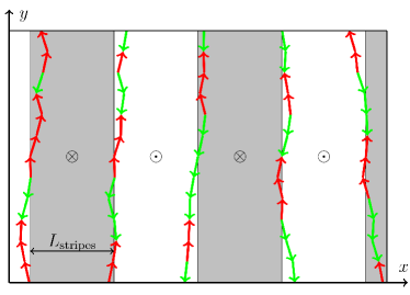
Figure 5: Schematic view of stripe pattern in a film with out-of-plane anisotropy. Gray and white areas represent domains with opposite magnetization in the ground state. Colored (online) arrows give a pictorial representation of DW corrugation and short-range chiral order at finite temperature. Note that Bloch DWs have been assumed and disorder in the arrows direction ($\varphi_{0}(y)$ variable) has been exaggerated to help visualization.

IV.2 Chiral order of domain walls

The instability with respect to $\varphi_{0}$ is, instead, related to DW chirality. As already pointed out, $\mathcal{Z}_{\varphi_{0}}$ may be thought of as arising from the 1d XY Hamiltonian given in Eq. (68) in the limit of small misalignment between neighboring chirality vectors $\vec{e}_{\varphi_{0}}(y)$. It is well-known that the 1d XY model – with nearest-neighbor interactions – can only sustain short-range order. Therefore, our picture suggests that just short-range chiral order should develop along the $y$ direction when only uniaxial anisotropy and exchange interaction are considered. An intermediate anisotropy $D_{x}\neq 0$ – for instance of magnetostatic origin – stabilizes two possible values of $\varphi_{0}$. Eventually, this drives the original XY Hamiltonian $\mathcal{H}_{\rm xy}$ in Eq. (68), which describes the effective coupling between chirality vectors, towards the Ising universality class. Neither in this case long-range chiral order along $y$ is expected to be stable. From a snapshot taken at finite temperature we would rather expect domains of opposite chirality to alternate randomly along, e.g., a Bloch DW (for which $\vec{e}_{\varphi_{0}}=(\pm 1,\,0,\,0)$). This phenomenon was recently observed on Fe/Ni/Cu(001) films Wu_PRL_2013 , consisting of 10 monolayers of Ni and 1.3 of Fe. Our conjecture is sketched pictorially in Fig. 5. Arrows represent the alternating magnetization direction along DWs, instead of the $\vec{e}_{\varphi_{0}}$ vectors, to facilitate the comparison with experiments reported in Ref. Wu_PRL_2013, . A scenario consistent with chiral order of DWs requires either a significant film thickness (so that dimensional crossover may occur) or the presence of a Dzyaloshinskii-Moriya interaction Wiesendanger_Nature_07 . The latter, still in Ref. Wu_PRL_2013, , was observed to stabilize homochiral Néel type of DWs, with $\vec{e}_{\varphi_{0}}=(0,\,1,\,0)$, in samples with thinner Ni interlayer.

Our considerations about short-range chiral order of DWs seem in striking contrast with Villain’s conjecture Villain_conj_78 (confirmed by experiments on Gd-based spin chains Cinti_PRL_08 ). This prescribes that in spin chains that develop short-range chiral order and are packed in a 3d crystal long-range chiral order should set in at higher temperature than magnetic ordering. In our mindset, the “information” about chirality of DWs in a 2d stripe-domain pattern cannot propagate along $x$, from one DW to the next because they are separated by regions in which all spins are aligned along the easy axis. Some misalignment between neighboring spins is, instead, needed to have a finite chiral order parameter. This ceases to hold true, e.g., close to the spin-reorientation transition where a canted-stripe phase was recently observed in 2d simulations Whitehead_PRB_08 ; Pighin_PRE_12 .

One should not forget that the arguments provided here strictly rely on thermodynamic equilibrium. Homochirality of DWs may be observed in experiments Niculin_PRB_10 ; Venus_PRB_10 ; Venus_PRB_11 and simulations as a result of slow dynamics Ana_PRE_13 ; Cannas_PRB_03 ; Kivelson_Phys_A_95 , similarly to what happens in superparamagnetic nanoparticles Brown63PR ; Brown79IEEE ; Cheng06PRL , for which long-range ferromagnetic order would be forbidden by equilibrium thermodynamics.

Chirality is also related to adiabatic spin transfer torque (STT), through which an electric current may displace a DW hosted in a ferromagnetic nanowire. Translation of the DW, i.e. a variation of the $x_{0}$ parameter, is in this case necessarily accompanied by a precession of the $\varphi_{0}$ angle, which produces a periodic change of the DW structure between Bloch and Néel type. The corresponding Landau-Lifshitz-Gilbert equation reads

$$\frac{{\rm d}\vec{S}}{{\rm d}t}=\gamma_{0}\vec{H}_{\rm eff}\times\vec{S}+\alpha_{\rm G}\vec{S}\times\frac{{\rm d}\vec{S}}{{\rm d}t}-u\,\partial_{x}\vec{S}$$ (75)

where the effective field is defined from the Hamiltonian $\mathcal{H}$ in Eq. (53) (possibly modified to include the magnetostatic energy or an intermediate anisotropy) as

$$\vec{H}_{\rm eff}=-\frac{1}{g\mu_{\rm B}}\frac{\delta\mathcal{H}}{\delta\vec{S}}\,,$$ (76)

$\gamma_{0}$ is the gyromagnetic ratio, $\alpha_{\rm G}$ the Gilbert damping and the last term accounts for the adiabatic STT with

$$u=\frac{g\mu_{\rm B}J_{\rm e}P}{2eM_{\rm s}\mathfrak{a}}\,;$$ (77)

in the equation above $J_{\rm e}$ represents the electrical current density and $P$ the polarization factor of the current (the lattice unit $\mathfrak{a}$ has been added because the derivative in Eq. (75) is considered dimensionless). In fact, the adiabatic STT contribution to the Landau-Lifshitz-Gilbert equation may be derived directly form the functional derivative in Eq. (76) if a contribution

$$\mathcal{H}_{\rm STT}=-\int\limits_{0}^{L_{y}+1}\mathrm{d}y\int\limits_{0}^{L_{x}+1}\vec{\Gamma}_{\rm STT}\cdot\left(\vec{S}\times\partial_{x}\vec{S}\right)\mathrm{d}x$$ (78)

is added to the Hamiltonian in Eq. (53). By analogy with standard Zeeman energy, Hamiltonian (78) alone would describe a precession of the local chirality vector B_Braun_AdvPhys_2012 $\vec{S}\times\partial_{x}\vec{S}$ about and effective “field” $\vec{\Gamma}_{\rm STT}=\tau u\vec{S}$. Due to its close relation with chirality, we believe that reconsidering adiabatic STT in the perspective of short-range chiral order may contribute to shed some light on the puzzling scenario of DW motion induced by electric currents. For instance, adiabatic STT seems to catch the main physics of Co/Ni nanowires magnetized out of plane Koyama_Nat_Mat_11 ; Koyama_IEEE_11 , while it largely fails for prototypical Permalloy nanowires (magnetized in plane) Thiaville_JAP_04 ; Thiaville_EPL_05 ; Yang_PRB_08 ; the critical current for DW motion is observed to depend strongly on temperature Malinowski_JPD_10 ; Curiale_PRL_12 in some samples and not in others Tanigawa_AppPhys_Ex_11 . Even if the extension to 2d of the sketch in Fig. 1 naturally leads to films or nanowires magnetized out-of-plane, our calculation can be adapted to samples magnetized in plane by a permutation of coordinates A_Mougin_EPL_07 ; Boulle_Mat_SEng_11 . Within our picture, the ratio between the correlation length characterizing short-range chiral order ($\xi_{\varphi_{0}}$) and the actual transverse size of a sample ($L_{y}$) should discriminate two regimes: for $\xi_{\varphi_{0}}\ll L_{y}$ the response of a DW to adiabatic STT is expected to depend strongly on temperature; for $\xi_{\varphi_{0}}\gg L_{y}$ this dependence should be much less dramatic. Also in this context, it is worth remarking that thermally-assisted DW depinning Burrowes_NatPhys_10 ; Martinez_JPCM_12 and possible non-homogeneous mechanisms of precession Zinoni_PRL_11 have been neglected in our considerations.

V Conclusions

We considered the effect of thermalized linear excitations about a DW profile. Expressions for the free energy of a DW embedded in 1d or 2d lattices were derived as a function of temperature and the system size. This was achieved by rephrasing in the language of Polyakov renormalization Polyakov ; Politi_EPL_94 ; Billoni_11 some known results, obtained from linearization of the Landau-Lifshitz equation Winter_61 ; Mikeska_JPC_83 ; Yan_11 ; Yan_12 ; Hertel-Kirschner_PRL04 ; Bayer_05 . Our approach is equivalent to the steepest-descent approximation of functional integrals Fogedby84JPCSSP . It has, in our opinion, the advantage of allowing for an easier generalization to 2d. Moreover, it provides a better insight on the role of fast- and slow-varying degrees of freedom, while keeping track of the non-homogeneity within the fluctuation field. For instance, it is straightforward to realize that fluctuations associated with bound states shall be localized at the DW center. This information might be relevant to the aim of accounting efficiently for thermal fluctuations in the Landau-Lifshitz-Gilbert equation wang_11 , beyond the mean-field level (Landau-Lifshitz-Bloch equation Nowak_PRB_09 ).

From the knowledge of the DW free energy, we provided a phenomenological expansion for the correlation length that may be used to fit the susceptibility of Single-Chain Magnets (slow-relaxing spin chains Miyasaka_review ; Coulon06Springer ; Bogani_JMC_08 ; Billoni_11 ; Gatteschi_Vindigni_13 ). The last ones are often realized by creating a preferential path for the exchange interaction between anisotropic magnetic units – consisting of transition metals or rare earths – through an organic radical. Thus, to some extent, Eq. (1) can be considered a reference Hamiltonian for Single-Chain Magnets in general Billoni_11 ; Gatteschi_Vindigni_13 .

In a previous work Ale_PRB_08 , we explained the shrinking of magnetic domains, observed in films with out-of-plane anisotropy, within a mean-field approach and assuming a non-homogeneous spin profile. Retaining the last feature for the unperturbed profile, in this paper we showed that Gaussian fluctuations also lead to a qualitatively similar result.

As a further implication, our model suggests that long-range chiral order cannot occur within DWs interposed between saturated domains. The robustness of this conjecture certainly deserves to be checked beyond the Gaussian approximation. Yet, it seems consistent with recent experiments on Fe/Ni/Cu(001) films Wu_PRL_2013 . This softening of chiral order may acquire some relevance also in view of DW manipulations by means of spin-transfer torque.

Appendix A Lowering and raising operators

In the next two Appendices we provide some details about the solution of the eigenvalue problem (6) in the presence of $\uparrow\downarrow$ b.c.. In terms of the lowering and raising operators

$$\begin{cases}&\hat{a}_{m}=\partial_{\eta}+m\tanh\eta\\ &\hat{a}^{\dagger}_{m}=-\partial_{\eta}+m\tanh\eta\,,\end{cases}$$ (79)

the generalized fluctuation Hamiltonian given in Eq. (23) reads $\hat{H}_{m}=\hat{a}^{\dagger}_{m}\hat{a}_{m}+m$. Using the commutator relation

$$[\hat{a}^{\dagger}_{m},\hat{a}_{m}]=-\frac{2m}{\cosh^{2}\eta}\,,$$ (80)

one finds the alternative representation $\hat{H}_{m}=\hat{a}_{m+1}\hat{a}^{\dagger}_{m+1}-(m+1)$. We now show that if $|\psi\rangle_{m}$ is an eigenstate of $\hat{H}_{m}$ then $\hat{a}^{\dagger}_{m+1}|\psi\rangle_{m}$ is an eigenstate of $\hat{H}_{m+1}$. Let $|\psi\rangle_{m}$ be an eigenstate of $\hat{a}_{m+1}\hat{a}^{\dagger}_{m+1}$ with eigenvalue $\lambda_{m}$, i.e. $\hat{a}_{m+1}\hat{a}^{\dagger}_{m+1}|\psi\rangle_{m}=\lambda_{m}|\psi\rangle_{m}$, then

$$\hat{a}^{\dagger}_{m+1}(\hat{a}_{m+1}\hat{a}^{\dagger}_{m+1}|\psi\rangle_{m}) =\hat{a}^{\dagger}_{m+1}\hat{a}_{m+1}(\hat{a}^{\dagger}_{m+1}|\psi\rangle_{m})$$ (81)

$$=\lambda_{m}(\hat{a}^{\dagger}_{m+1}|\psi\rangle_{m})\,,$$ (82)

which means that $\hat{a}^{\dagger}_{m+1}|\psi\rangle_{m}$ is an eigenstate of $\hat{a}^{\dagger}_{m+1}\hat{a}_{m+1}$ with the same eigenvalue $\lambda_{m}$. With the above representations of $\hat{H}_{m}$ and $\hat{H}_{m+1}$, it can easily be checked that if $|\psi\rangle_{m}$ is an eigenstate of $\hat{H}_{m}$ with eigenvalue $\mathcal{E}_{m}$ then $\hat{a}^{\dagger}_{m+1}|\psi\rangle_{m}$ is an eigenstate of $\hat{H}_{m+1}$ with eigenvalue $\mathcal{E}_{m}+2(m+1)$. Thus, the Hamiltonians $\hat{H}_{m}$ and $\hat{H}_{m+1}$ share the same spectrum, except for the fact that $\hat{H}_{m+1}$ has the additional eigenstate $|0\rangle_{m+1}$, defined by $\hat{a}_{m+1}|0\rangle_{m+1}=0$, which is not present in the spectrum of $\hat{H}_{m}$. This property allows constructing eigenstates of the Hamilton operator $\hat{H}_{m}$ recursively. For the case of our interest, we stop the iteration at the first step $m=1$, namely we just apply $\hat{a}^{\dagger}_{1}$ to the free-particle eigenstates (see the following Appendix for the explicit calculation). The missing vacuum state $|0\rangle_{1}$ is nothing but the bound state represented through Eq. (25) in real space.

Appendix B Derivation of the density of states

In the finite system, the solutions of the free–particle Hamiltonian are $\psi_{0}(q,x)=A\cos(qx)+B\sin(qx)$, where $A\,,B$ are constants to be determined from the boundary and normalization conditions. The free–state solutions of the Schrödinger–like Eq. (6) obtained for antiperiodicity b.c. (namely when $\vec{n}(x)$ describes a DW profile) can be obtained by applying the raising operator $\hat{a}^{\dagger}_{1}$ defined in Eq. (24) to $\psi_{0}(q,x)$:

$$\begin{split}\Phi_{a,q}(x)=&A\left[q\sin(qx)/c+\tanh(c(x-x_{0}))\cos(qx)\right]\\ &+B\left[\tanh(c(x-x_{0}))\sin(qx)-q\cos(qx)/c\right]\,,\end{split}$$ (83)

with $a=x_{0},\varphi_{0}$. Independently of the determination of $A$ and $B$, it is straightforward to show that $\Phi_{a,q}(x)$ are solutions of the Schrödinger-like Eq. (6) with eigenvalues

$$\varepsilon_{a,q}=\frac{J}{2}q^{2}+D\,,$$ (84)

formally equal to those obtained starting from a uniform profile ($\uparrow\uparrow$ b.c.). We show in the following that the allowed values of $q$ are not the same, which affects the density of states.
The constants $A$ and $B$ in Eq. (83) have to be determined from the boundary conditions $\Phi_{a,q}(0)=\Phi_{a,q}(L+1)=0$ and the normalization condition

$$\int\limits_{0}^{L+1}\mathrm{d}x\,|\Phi_{a,q}(x)|^{2}=1\,.$$ (85)

Though deriving an analytic expression for $A$ and $B$ is computationally demanding, the density of states can easily be obtained. Non-trivial solutions ($A\neq 0$ and $B\neq 0$) exist only if the determinant of the system defined by the boundary conditions $\Phi_{a,q}(0)=\Phi_{a,q}(L+1)=0$ vanishes:

$$\begin{split}&\tanh(cx_{0})\tanh\left(c(L+1-x_{0})\right)\tan{q(L+1)}\\ &-q\tanh(cx_{0})/c-q^{2}\tan{c(L+1-x_{0})}/c^{2}\\ &-q\tanh\left(c(L+1-x_{0})\right)/c=0\,,\end{split}$$ (86)

which gives the following transcendental equation for the determination of the possible $q$ values

$$\tan{q(L+1)}=\frac{q\left(\tanh(cx_{0})+\tanh\left(c(L+1-x_{0})\right)\right)}{c\left(\tanh(cx_{0})\tanh\left(c(L+1-x_{0})\right)-q^{2}/c^{2}\right)}\,.$$ (87)

This equation can be solved using, e.g., graphical methods. More significantly, it allows deriving an analytic expression for the density of states. To this purpose, let us set

$$\tan{\alpha}=\frac{q\left(\tanh(cx_{0})+\tanh\left(c(L+1-x_{0})\right)\right)}{c\left(\tanh(cx_{0})\tanh\left(c(L+1-x_{0})\right)-q^{2}/c^{2}\right)}\,.$$ (88)

The solution of Eq. (87) is

$$\begin{cases}&q(L+1)=\alpha+p\pi\qquad\mathrm{with}\quad p\in\mathbb{Z}\\ &\alpha=\arctan\left[\frac{q\left(\tanh(cx_{0})+\tanh\left(c(L+1-x_{0})\right)\right)}{c\left(\tanh(cx_{0})\tanh\left(c(L+1-x_{0})\right)-q^{2}/c^{2}\right)}\right]\end{cases}$$ (89)

which can be solved for $p$ to obtain

$$\begin{split}&p=\frac{q(L+1)}{\pi}\\ &-\frac{1}{\pi}\arctan\left[\frac{q\left(\tanh(cx_{0})+\tanh\left(c(L+1-x_{0})\right)\right)}{c\left(\tanh(cx_{0})\tanh\left(c(L+1-x_{0})\right)-q^{2}/c^{2}\right)}\right]\,.\end{split}$$ (90)

The density of states Currie_PRB_80 is defined as

$$\begin{split}\rho(q)&=\frac{{\rm d}p}{{\rm d}q}=\frac{L+1}{\pi}-\frac{c}{\pi}\left[\tanh(cx_{0})\tanh\left(c(L+1-x_{0})\right)+\frac{q^{2}}{c^{2}}\right]\\ &\times\frac{\tanh(cx_{0})+\tanh\left(c(L+1-x_{0})\right)}{\Delta(q,x_{0})}\,,\qquad\mathrm{with}\\ &\Delta(q,x_{0})=c^{2}\left(\tanh(cx_{0})\tanh\left(c(L+1-x_{0})\right)-\frac{q^{2}}{c^{2}}\right)^{2}\\ &+q^{2}\left[\tanh(cx_{0})+\tanh\left(c(L+1-x_{0})\right)\right]^{2}\,.\end{split}$$ (91)

In order to compute the DW free energy analytically, we assume the DW to be centered in the system, i.e., $x_{0}=(L+1)/2$. In this case, Eq. (87) reads

$$\tan[q(L+1)]=\frac{2q\tanh\left(c(L+1)/2\right)}{c\left(\tanh^{2}(c(L+1)/2)-q^{2}/c^{2}\right)}\,.$$ (92)

Setting $\tan\alpha=q/c\tanh(c(L+1)/2)$, Eq. (92) takes the form

$$\tan[q(L+1)]=\tan(2\alpha)\,.$$ (93)

The density of states simplifies to

$$\rho(q)=\frac{L+1}{\pi}-\frac{2c\tanh(c(L+1)/2)}{\pi(c^{2}\tanh^{2}(c(L+1)/2)+q^{2})}\,,$$ (94)

and for $L\gg 1/c$, $\tanh^{2}(c(L+1)/2)\approx 1$,

$$\rho(q)=\frac{L+1}{\pi}-\frac{2c}{\pi(c^{2}+q^{2})}\,.$$ (95)

In order to check the validity of Eq. (94), we performed a numerical diagonalization of Eq. (6) for a finite, discrete lattice (the excellent agreement is summarized in Fig. 6).

Diagonalization of the discrete eigenvalue problem
The discrete version of Eq. (6) is given by

$$\sum_{j,k}\psi(j)\left[-\frac{J}{2}\Delta_{j,k}+V(k)\delta_{j,k}\right]\psi(k)=\varepsilon\,,$$ (96)

where $\Delta_{j,k}$ is the discrete Laplace operator

$$\Delta_{j,k}=\begin{cases}-2&j=k\\ 1&k=j\pm 1\\ 0&\mathrm{else}\end{cases}\,,$$ (97)

the potential is

$$\begin{cases}V(k)=D\left(2\cos^{2}(\theta_{k})-1\right)&\quad{\rm for}\quad\uparrow\downarrow\,{\rm b.c.}\\ V(k)=D&\quad{\rm for}\quad\uparrow\uparrow\,{\rm b.c.}\,,\end{cases}$$ (98)

and $\theta_{k}$ corresponds to the discrete profile computed, e.g., with the non-linear map method (see Appendix D). A complete orthonormal system fulfilling the boundary conditions $\psi(0)=\psi(L+1)=0$ is

$$u_{n}(j)=\sqrt{\frac{2}{L+1}}\sin(q_{n}j)\qquad\qquad q_{n}=\frac{\pi}{L+1}n$$ (99)

with $0\leq j\leq L+1$ and $1\leq n\leq L$. The functions $\psi$ are expanded in this basis

$$\psi(j)=\sum_{n}w_{n}u_{n}(j)$$ (100)

and inserted into Eq. (96) to get

$$\sum_{n,m}w_{n}\left[J(1-\cos(q_{n}))\delta_{n,m}+M_{n,m}\right]w_{m}=\varepsilon\,,$$ (101)

with

$$M_{n,m}=\sum_{j}u_{n}(j)V(j)u_{m}(j)\,.$$ (102)

This is equivalent to solving the eigenvalue problem

$$\sum_{m}\left[J(1-\cos(q_{m}))\delta_{n,m}+M_{n,m}\right]w_{m}=\varepsilon_{n}w_{n}\,.$$ (103)

It is worth noting that in a finite discrete system the possible number of eigenfunctions $L$ is finite. As a consequence, every time a domain wall is added, a free state is “lost” and a bound state is “gained”. However, this procedure is correct only when the distance between DWs is large enough to treat them independently. In our case we just considered one or no DW in the system. When no DW is present, i.e. for $\uparrow\uparrow$ b.c., $u_{n}(j)$ are solutions to the eigenvalue problem in Eq. (96) with eigenvalues

$$\varepsilon_{\uparrow\uparrow,n}=J(1-\cos(q_{n}))+D\,.$$ (104)

As already mentioned, the dispersion relation is expected to depend on $q$ in the same way for both choices of b.c., but the allowed values of $q$ may – generally – be different. The spectrum in Eq. (104) was compared with that obtained by solving the eigenvalue problem (103) numerically: $\varepsilon_{n}$ obtained in both cases were plotted against the eigenvalue index $n$. Indeed, the two dispersion relations turned out to overlap. Therefore, the “shifted” $q_{\uparrow\downarrow,n}$, corresponding to $\uparrow\downarrow$ b.c., could be deduced through the following formula:

$$q_{\uparrow\downarrow,n}=\arccos\left(\frac{J+D-\varepsilon_{\uparrow\downarrow,n}}{J}\right)\,.$$ (105)

Eventually, the density of states was obtained with the discrete derivative

$$\rho(q)=\frac{\partial n}{\partial q}\simeq\frac{1}{q_{\uparrow\downarrow,n+1}-q_{\uparrow\downarrow,n}}\,.$$ (106)

Figure 6: (Color online). Density of states $\rho(q)=\partial n/\partial q$ for $D/J=0.01$ and $L=99$. For small values of $q$ the density is decreased with respect to $\rho_{\uparrow\uparrow}=100/\pi$, expected for a uniform $\vec{n}$, due to DW–spin wave interaction.

Symbols in Fig. 6 represent the resulting density of states. Analytic results are drawn with lines: the (blue) short-dashed line corresponds to Eq. (95) while the (green) solid line to $\rho_{\uparrow\uparrow}=(L+1)/\pi$. Indeed, Eq. (95) agrees very well with the numerical calculation.

Appendix C Scaling of the correlation length

In this Appendix we describe the way in which a semi-analytical expression for the correlation length was deduced. As mentioned in the main text and shown in Fig. 3, a better agreement between $\Delta F$ given in Eq. (33) and numerical results is obtained by introducing the renormalized parameters $D(\lambda_{\rm c})$ and $c(\lambda_{\rm c})$ only in the argument of the logarithm. Considering that $D(\lambda_{\rm c})=D\,Z^{3}(\lambda_{\rm c})$ and $c(\lambda_{\rm c})=c\,Z(\lambda_{\rm c})$, after this substitution, the DW free energy takes the form

$$\Delta F=\mathcal{E}_{\rm dw}-T\log\left\{\beta\mathcal{E}_{\rm dw}cLZ^{3}\left[1+\tanh(cZ(L+1)/2)\right]^{2}\right\}\,.$$ (107)

We are interested in the value of $L=\bar{L}$ for which $\Delta F(\bar{L})=0$. Let us set $\tilde{\xi}=c\bar{L}$ and $\zeta=\beta\mathcal{E}_{\rm dw}$ so that our problem reduces to an implicit equation in the variables $\tilde{\xi}$ and $\zeta$. Then consider the following map in the $\tilde{\xi}$ variable

$$\begin{split}&\Xi_{it}=\frac{Z(\zeta)}{2}(\tilde{\xi}_{it}+c)\\ &\tilde{\xi}_{it+1}=\frac{{\rm e}^{\zeta}}{\zeta Z^{3}(\zeta)}\left[1+\tanh(\Xi_{it})\right]^{-2}\end{split}$$ (108)

parametrically dependent on $\zeta$, with $it=1,2,\dots$ representing the iteration index. From its definition it follows that $Z(\lambda_{\rm c})=Z(\zeta)=1-1/\zeta$. The initial condition of the map (108) is set to

$$\tilde{\xi}_{1}=\frac{{\rm e}^{\zeta}}{4\zeta Z^{3}(\zeta)}\,.$$ (109)

The fixed point $\tilde{\xi}_{\infty}$ gives the sought for solution $\Delta F(\bar{L})=0$. For $\tilde{\xi}_{1}\gg 1$, it is $\Xi_{1}\gg 1$ and $\tanh(\Xi_{1})\simeq 1$, consequently. In this case the map converges already at the first iteration, namely $\tilde{\xi}_{1}\simeq\tilde{\xi}_{\infty}$. Numerically one finds that the latter equivalence holds within 1.4% for any $D/J>0.1$.
To extend the validity of Eq. (109) to high temperatures we used the trick – not fully justified – that Polyakov renormalization somehow stops when $\lambda_{\rm c}=\bar{L}/2-3/2c$. In terms of the reduced variable entering the map (108), this happens when $\tilde{\xi}_{\infty}=2\pi+3$, which occurs at $\zeta=4.262$. We are now in the position to give an expression for the scaling function $f(\zeta)$ describing the universal behavior of the product $c\,\xi$ as a function of the scaling variable $\zeta=\beta\mathcal{E}_{\rm dw}$:

$$f(\zeta)=\begin{cases}\frac{{\rm e}^{\zeta}}{4\zeta Z^{3}(\zeta)}&\quad{\rm for}\,\,\,\zeta>4.262\\ &\\ A_{0}\,{\rm e}^{b\zeta+1}&\quad{\rm otherwise}\end{cases}$$ (110)

with constants $A_{0}=0.3282$ and $b=0.5496$ determined by requiring the continuity of $\tilde{\xi}_{1}$ and its derivative with respect to $\zeta$. The exact relation between the scaling function $f(\zeta)$ and $\xi$ computed numerically can only be obtained by fitting a constant prefactor (see Fig. 3); we already pointed out that this is of the order of the Euler constant so that we can reasonably set the equivalence $c\,\xi\simeq f(\zeta)/{\rm e}$.

Appendix D Spin profile in laterally constrained domain walls

Here we repropose an analytic derivation of the DW profile for finite systems B_Braun_AdvPhys_2012 ; B_Braun_JAP_2006 – which employs a continuum formalism – and check its results against numerical calculations on a discrete lattice.
We first consider the DW profile for an infinite chain with $\uparrow\downarrow$ b.c.. Since for $T=0$ one has $\vec{n}(x)=\vec{S}(x)$, the minimum-energy profile given in Eq. (18) can be obtained from Hamiltonian (2). The latter in polar coordinates $\vec{S}\equiv(\sin\theta\cos\varphi,\sin\theta\sin\varphi,\cos\theta)$ reads

$$\begin{split}\mathcal{H}&=\int\frac{J}{2}\left[\left(\partial_{x}\theta\right)^{2}+\sin^{2}(\theta)\left(\partial_{x}\varphi\right)^{2}\right]\,\mathrm{d}x\\ &-\int\left[D\cos^{2}(\theta)+D_{x}\sin^{2}(\theta)\cos^{2}(\varphi)\right]\,\mathrm{d}x+\mathrm{const}\,.\end{split}$$ (111)

The intermediate anisotropy $D_{x}$ such that $0<|D_{x}|<|D|$ has been introduced for the sake of generality. The profile which minimizes the functional in Eq. (111) with respect to $\theta(x)$ and $\varphi(x)$ is the solution to the following Euler–Lagrange equations

$$\begin{split}&\bullet\quad J\partial_{x}^{2}\theta=J\sin\theta\cos\theta\left(\partial_{x}\varphi\right)^{2}+2\tilde{D}\cos\theta\sin\theta\\ &\bullet\quad J\sin^{2}(\theta)\partial_{x}^{2}\varphi+2J\sin\theta\cos\theta\partial_{x}\theta\partial_{x}\phi\\ &\quad\quad=2D_{x}\sin^{2}(\theta)\sin\varphi\cos\varphi\end{split}$$ (112)

(where $\tilde{D}=D-D_{x}\cos^{2}(\varphi)$) compatible with $\uparrow\downarrow$ b.c., that is

$$\begin{split}&\cos\left(\theta(x)\right)=-\tanh(c(x-x_{0}))\\ &\varphi(x)=\varphi_{0}=0,\frac{\pi}{2},\pi,\frac{3\pi}{2}\,,\end{split}$$ (113)

with the more general $c=\sqrt{2\tilde{D}/J}$ than in the main text. The choice of $\varphi_{0}$ depends on the sign of the intermediate anisotropy. For $D_{x}>0$ one has $\varphi_{0}=0,\pi$ (Néel DW), while for $D_{x}<0$ it is $\varphi_{0}=\pi/2,3\pi/2$ (Bloch DW). Note that in both cases there exist two degenerate solutions which correspond to opposite chirality of the DW B_Braun_AdvPhys_2012 . The energy associated with the profile (113) – with respect to a uniform ground state – is $\mathcal{E}_{\rm dw}=2\sqrt{2\tilde{D}J}-D_{x}$.

A helpful, well-established Leung_82 analogy consists in interpreting $x$ as “time” and $\theta$ as “spatial coordinate”. Then the first Euler–Lagrange equation in (LABEL:eq:219) describes the motion of a classical particle of “mass” $J$ moving in a potential $V(\theta)=D\cos^{2}(\theta)+D_{x}\sin^{2}(\theta)\cos^{2}(\varphi_{0})$ ($\varphi=\varphi_{0}$ has been assumed). The “particle energy”

$$\varepsilon=\frac{J}{2}(\partial_{x}\theta)^{2}+\frac{\tilde{D}}{2}\cos(2\theta)$$ (114)

is a constant of integration and it is univocally defined by the b.c.

$$\begin{cases}&\theta(0)=0\\ &\theta(L+1)=\pi\,,\end{cases}$$ (115)

consistent with Fig. 1. For the infinite chain $\theta(-\infty)=0$ and $\theta(\infty)=\pi$, which yields $\varepsilon=D/2$, namely $\partial_{x}\theta=0$ at the boundaries. For finite chains, instead, one expects $\varepsilon>D/2$, i.e., a non-vanishing derivative at the boundaries. We will see that this condition is necessary to develop a continuum model for finite chains (it guarantees the convergence of the elliptic integrals in Eqs. (116)–(117)). Integration of Eq. (114) gives the following implicit equation for the DW profile

$$x=\sqrt{\frac{J}{\tilde{D}}}\int\limits_{0}^{\theta}\,\frac{\mathrm{d}\theta^{\prime}}{\sqrt{\frac{2\varepsilon}{\tilde{D}}-\cos(2\theta^{\prime})}}$$ (116)

where the b.c. $\theta(0)=0$ has been used. The second b.c. in Eq. (115) implies

$$L+1=2\sqrt{\frac{J}{2\varepsilon+\tilde{D}}}\,\,\mathcal{K}\left(\sqrt{\frac{2\tilde{D}}{2\varepsilon+\tilde{D}}}\right)\,,$$ (117)

$\mathcal{K}$ being the complete elliptic integral of the first kind. This equation can be solved numerically to deduce $\varepsilon$. The whole model holds for broad DWs, $c\ll 1$, when the continuum limit is appropriate. Numerical instabilities are expected for $\varepsilon\simeq\tilde{D}/2$, when integrals diverge. Assuming that the DW is centered at $(L+1)/2$ with $\theta((L+1)/2)=\pi/2$, the spin profile can also be computed as

$$x=\frac{L+1}{2}-\sqrt{\frac{J}{\tilde{D}}}\int\limits_{\theta}^{\pi/2}\,\frac{\mathrm{d}\theta^{\prime}}{\sqrt{\frac{2\varepsilon}{\tilde{D}}-\cos(2\theta^{\prime})}}$$ (118)

which solves the possible numerical divergence at the boundaries. Though Eq. (118) only applies to $x\leq(L+1)/2$, the other half of the profile can be deduced from the property $\theta(L+1-x)=\pi-\theta(x)$. For very short chains the constant of integration is approximately $\varepsilon=J(\partial_{x}\theta)^{2}/2$ (meaning that in Eq. (114) the derivative dominates over the cosine term also at boundaries). As a consequence, the condition (117) takes the form

$$L+1=\sqrt{\frac{J}{2\varepsilon}}\int\limits_{0}^{\pi}\mathrm{d}\theta\,,$$ (119)

which gives $\varepsilon=J(\pi/(L+1))^{2}/2$, i.e., the derivative $\partial_{x}\theta$ is constant over the whole chain and takes the value of the smallest wave-vector $q$ allowed in the reciprocal space. The spin profile can be computed analytically

$$\theta(x)=\frac{\pi}{L+1}x\quad\Rightarrow\quad S^{z}(x)=\cos\left(\frac{\pi}{L+1}x\right)\,.$$ (120)

The above profile corresponds to a single harmonic. In Figure 7, the spin profile obtained with different methods (at $T=0$) for two different chain lengths is shown. The harmonic approximation is satisfactory for $L=6$ but – as expected – does not reproduce the discrete-lattice calculation for $L=150$ (not shown).

Figure 7: (Color online). DW spin profile obtained with different methods for $D/J=0.05$, yielding $c^{-1}\approx 3.16$. Non–linear map and continuum approach produce the same spin profile for both $L=6,\,150$. For $L=6$, the harmonic approximation given by Eq. (120) is also accurate.

Discrete-lattice calculation
In the case of a discrete chain, a recursion formula (non–linear map) for the computation of the spin profile was proposed in Refs. trallori:94, ; rettori:95, ; trallori:96, . The starting point is the DW Hamiltonian

$$\mathcal{H}_{\rm dw}=J\sum_{i=0}^{L}\left(1-\cos\left(\theta_{i+1}-\theta_{i}\right)\right)+\sum_{i=0}^{L+1}D\sin^{2}(\theta_{i})\,,$$ (121)

where the decomposition

$$\vec{S}_{i}\cdot\vec{S}_{j}=\cos(\theta_{i})\cos(\theta_{j})+\sin(\theta_{i})\sin(\theta_{j})\cos(\varphi_{i}-\varphi_{j})$$ (122)

with $\varphi_{i}=\varphi_{0}$ was used. To find the profile, $\mathcal{H}_{\rm dw}$ has to be minimized

$$\frac{\partial\mathcal{H}_{\rm dw}}{\partial\theta_{i}}=0\,,\qquad\qquad 0<i<L+1$$ (123)

which yields

$$J\sin(\theta_{i}-\theta_{i-1})-J\sin(\theta_{i+1}-\theta_{i})+D\sin(2\theta_{i})=0\,.$$ (124)

The non-linear map is built as follows

$$\tilde{s}_{i+1}=\sin(\theta_{i+1}-\theta_{i})\,,$$ (125)

so that

$$\tilde{s}_{i+1}=\tilde{s}_{i}+\frac{D}{J}\sin(2\theta_{i})\,,$$ (126)

and

$$\theta_{i+1}=\theta_{i}+\arcsin(\tilde{s}_{i+1})\,.$$ (127)

The procedure gives a unique solution, when the boundary conditions are inserted

$$\theta_{0}=0\qquad\qquad\qquad\theta_{L+1}=\pi\,,$$ (128)

and the first step is given, $\theta_{L}=\pi-\delta$. The difficulty of the procedure is to find the correct value of $\delta$ which satisfies the boundary conditions (128). In practice, one tries different values of $\delta$ until $|\theta_{0}|$ is smaller than a preset threshold. However, this procedure gets numerically unstable for long chains. For $L$ odd, one can circumvent the problem by letting the iteration start at the DW center, where $\theta_{(L+1)/2}=\pi/2$ and $\theta_{(L+3)/2}=\pi/2+\delta$. The more dramatic misalignment between two adjacent spins occurs at the DW center. Therefore here the iteration step $\delta$ can be defined more easily. After a certain iteration $\bar{i}$, all the spins characterized by a lattice index $i>\bar{i}$ are assumed to point along the same direction as the boundary, $\theta_{i}=\pi$. The configuration of spins lying on the other side of the DW one has is obtained from the condition

$$\theta_{L+1-i}=\pi-\theta_{i}\qquad(L+1)/2<i\leq L+1$$ (129)

Figure 7 shows that the results obtained with the non-linear map (for a discrete lattice) and those computed with the continuum formalism (by means of Eqs. (117) and (118)) are not distinguishable.

References

- (1) J. C. Slonczewski, J. Magn. Magn. Mater. 159, L1 (1996)
- (2) S. S. P. Parkin, M. Hayashi, and L. Thomas, Science 320, 190 (2008)
- (3) M. Hayashi, L. Thomas, R. Moriya, C. Rettner, and S. S. P. Parkin, Science 320, 209 (2008)
- (4) D. A. Allwood, G. Xiong, C. C. Faulkner, D. Atkinson, D. Petit, and R. P. Cowburn, Science 309, 1688 (2005)
- (5) A. Vanhaverbeke, A. Bischof, and R. Allenspach, Phys. Rev. Lett. 101, 107202 (2008)
- (6) G. Chen, J. Zhu, A. Quesada, J. Li, A. T. N’Diaye, Y. Huo, T. P. Ma, Y. Chen, H. Y. Kwon, C. Won, Z. Q. Qiu, A. K. Schmid, and Y. Z. Wu, Phys. Rev. Lett. 110, 177204 (2013)
- (7) P. Fischer, D.-H. Kim, B. L. Mesler, W. Chao, A. E. Sakdinawat, and E. H. Anderson, Surf. Sci. 601, 4680 (2007)
- (8) G. Tatara and H. Kohno, Phys. Rev. Lett. 92, 086601 (2004)
- (9) O. A. Tretiakov and A. Abanov, Phys. Rev. Lett. 105, 157201 (2010)
- (10) O. A. Tretiakov, Y. Liu, and A. Abanov, Phys. Rev. Lett. 105, 217203 (2010)
- (11) Y. Tserkovnyak and D. Loss, Phys. Rev. Lett. 108, 187201 (2012)
- (12) Z. Yuan, Y. Liu, A. A. Starikov, P. J. Kelly, and A. Brataas, Phys. Rev. Lett. 109, 267201 (2012)
- (13) C. Schieback, D. Hinzke, M. Kläui, U. Nowak, and P. Nielaba, Phys. Rev. B 80, 214403 (2009)
- (14) E. Martinez, L. Lopez-Diaz, O. Alejos, L. Torres, and M. Carpentieri, Phys. Rev. B 79, 094430 (2009)
- (15) E. Martinez, J. Phys.: Condens. Matter 24, 024206 (2012)
- (16) H. C. Fogedby, P. Hedegard, and A. Svane, J. Phys. C: Solid State Phys. 17, 3475 (1984)
- (17) K. M. Leung, Phys. Rev. B 26, 226 (1982)
- (18) K. Nakamura and T. Sasada, Solid St. Commun. 21, 891 (1977)
- (19) K. Nakamura and T. Sasada, J. Phys. C: Solid State Phys. 11, 331 (1978)
- (20) J. A. Krumhansl and J. R. Schrieffer, Phys. Rev. B 11, 3535 (1975)
- (21) J. M. Winter, Phys. Rev. 124, 452 (1961)
- (22) C. Etrich and H. J. Mikeska, J. Phys. C: Solid State Phys. 16, 4889 (1983)
- (23) P. Yan, X. S. Wang, and X. R. Wang, Phys. Rev. Lett. 107, 177207 (2011)
- (24) P. Yan and G. E. W. Bauer, Phys. Rev. Lett. 109, 087202 (2011)
- (25) R. Hertel, W. Wulfhekel, and J. Kirschner, Phys. Rev. Lett. 93, 257202 (2004)
- (26) C. Bayer, H. Schultheiss, B. Hillebrands, and R. L. Stamps, IEEE Trans. Magn. 10, 3094 (2005)
- (27) H. Miyasaka, M. Julve, M. Yamashita, and R. Clérac, Inorg. Chem. 48, 3420 (2009)
- (28) C. Coulon, H. Miyasaka, and R. Clérac, Struct. Bond. 122, 163 (2006)
- (29) L. Bogani, A. Vindigni, R. Sessoli, and D. Gatteschi, J. Mater. Chem. 18, 4750 (2008)
- (30) O. V., Billoni, V. Pianet, D. Pescia, and A. Vindigni, Phys. Rev. B 84, 064415 (2011)
- (31) D. Gatteschi and A. Vindigni, (2013), arXiv:1303.3731
- (32) O. Boulle, G. Malinowski, and M. Kläui, Mater. Sci. Eng. R 72, 159 (2011)
- (33) H.-B. Braun, Phys. Rev. B 50, 16485 (1994)
- (34) O. Portmann, A. Vaterlaus, and D. Pescia, Phys. Rev. Lett. 96, 047212 (2006)
- (35) N. Saratz, A. Lichtenberger, O. Portmann, U. Ramsperger, A. Vindigni, and D. Pescia, Phys. Rev. Lett. 104, 077203 (2010)
- (36) A. Vindigni, N. Saratz, O. Portmann, D. Pescia, and P. Politi, Phys. Rev. B 77, 092414 (2008)
- (37) A. M. Polyakov, Phys. Lett. B 59, 79 (1975)
- (38) P. Politi, A. Rettori, M. G. Pini, and D. Pescia, Europhys. Lett. 28, 71 (1994)
- (39) J. F. Currie, J. A. Krumhansl, A. R. Bishop, and S. E. Trullinger, Phys. Rev. B 22, 447 (1980)
- (40) H.-B. Braun, Adv. Phys. 61, 1 (2012)
- (41) R. Ishikawa, K. Katoh, B. K. Breedlove, and M. Yamashita, Inorg. Chem. 51, 9123 (2012)
- (42) M. Balanda, M. Rams, S. K. Nayak, Z. Tomkowicz, W. Haase, K. Tomala, and J. V. Yakhmi, Phys. Rev. B 74, 224421 (2006)
- (43) W.-X. Zhang, R. Ishikawa, B. Breedlove, and M. Yamashita, RSC Adv. 3, 3772 (2013)
- (44) A. R. McGurn and D. J. Scalapino, Phys. Rev. B 11, 2552 (1975)
- (45) M. Blume, P. Heller, and N. A. Lurie, Phys. Rev. B 11, 4483 (1975)
- (46) R. Pandit and C. Tannous, Phys. Rev. B 28, 281 (1983)
- (47) A. Vindigni, A. Rettori, M. Pini, C. Carbone, and P. Gambardella, Appl. Phys. A 82, 385 (Feb. 2006)
- (48) H. W. Wyld, Mathematical Methods of Physics (Benjamin, Massachusetts, USA, 1976)
- (49) M. E. Fisher, Am. J. Phys. 32, 343 (1964)
- (50) A. H. Stroud, Approximate Calculation of Multiple Integrals (Prentice-Hall, Englewood Cliffs, New Jersey, USA, 1971)
- (51) A. D. McLaren, Math. Comp. 17, 361 (1963)
- (52) M. Abramowitz and I. E. Stegum, Handbook of mathematical functions (Dover, New York, USA, 1970)
- (53) L. Trallori, P. Politi, A. Rettori, M. G. Pini, and J. Villain, Phys. Rev. Lett. 72, 1925 (1994)
- (54) A. Rettori, L. Trallori, P. Politi, M. G. Pini, and M. Macciò, J. Mag. Mag. Mater. 140–144, 639 (1995)
- (55) L. Trallori, M. G. Pini, A. Rettori, M. Macciò, and P. Politi, Int. J. Mod. Phys. B 10, 1935 (1996)
- (56) S. A. Pighin, O. V. Billoni, and S. A. Cannas, Phys. Rev. E 86, 051119 (2012)
- (57) A. B. MacIsaac, J. P. Whitehead, M. C. Robinson, and K. De’Bell, Phys. Rev. B 51, 16033 (1995)
- (58) S. A. Pighin, O. V. Billoni, D. A. Stariolo, and S. A. Cannas, Phys. Rev. E 322, 3889 (2010)
- (59) A. Giuliani, J. L. Lebowitz, and E. H. Lieb, Phys. Rev. B 76, 184426 (2007)
- (60) A. Giuliani, J. L. Lebowitz, and E. H. Lieb, Phys. Rev. B 84, 064205 (2011)
- (61) O. Portmann, A. Gölzer, N. Saratz, O. V. Billoni, D. Pescia, and A. Vindigni, Phys. Rev. B 82, 184409 (2010)
- (62) A. Abanov, V. Kalatsky, V. L. Pokrovsky, and W. M. Saslow, Phys. Rev. B 51, 1023 (1995)
- (63) A. B. Kashuba and V. L. Pokrovsky, Phys. Rev. B 48, 10335 (1993)
- (64) D. G. Barci, L. Ribeiro, and D. A. Stariolo, Phys. Rev. E 87, 062119 (2013)
- (65) S. A. Cannas, M. F. Michelon, D. A. Stariolo, and F. A. Tamarit, Phys. Rev. B 73, 184425 (2006)
- (66) J. Toner and D. R. Nelson, Phys. Rev. B 23, 316 (1981)
- (67) S. Brazovskii and T. Nattermann, Adv. Phys. 53, 177 (2004)
- (68) S. Lemerle, J. Ferré, C. Chappert, V. Mathet, T. Giamarchi, and P. Le Doussal, Phys. Rev. Lett. 80, 849 (1998)
- (69) K.-J. Kim, J.-C. Lee, S.-M. Ahn, K.-S. Lee, C.-W. Lee, Y. J. Cho, S. Seo, K.-H. Shin, S.-B. Choe, and H.-W. Lee, Nature 458, 740 (2009)
- (70) M. Bode, M. Heide, K. von Bergmann, P. Ferriani, S. Heinze, G. Bihlmayer, A. Kubetzka, O. Pietzsch, S. Blügel, and R. Wiesendanger, Nature 447, 190 (2007)
- (71) J. Villain, in Proceedings of the 13th IUPAP Conference on Statistical Physics[Ann. Isr. Phys. Soc. 2, 565 (1978)](1978)
- (72) F. Cinti, A. Rettori, M. G. Pini, M. Mariani, E. Micotti, A. Lascialfari, N. Papinutto, A. Amato, A. Caneschi, D. Gatteschi, and M. Affronte, Phys. Rev. Lett. 100, 057203 (2008)
- (73) J. P. Whitehead, A. B. MacIsaac, and K. De’Bell, Phys. Rev. B 77, 174415 (2008)
- (74) N. Saratz, U. Ramsperger, A. Vindigni, and D. Pescia, Phys. Rev. B 82, 184416 (2010)
- (75) N. Abu-Libdeh and D. Venus, Phys. Rev. B 81, 195416 (2010)
- (76) N. Abu-Libdeh and D. Venus, Phys. Rev. B 84, 094428 (2011)
- (77) A. C. Ribeiro Teixeira, D. A. Stariolo, and D. G. Barci, Phys. Rev. E 87, 062121 (2013)
- (78) P. M. Gleiser, F. A. Tamarit, S. A. Cannas, and M. A. Montemurro, Phys. Rev. B 68, 134401 (2003)
- (79) D. Kivelson, S. A. Kivelson, X. Zhao, Z. Nussinov, and T. G., Phys. A 219, 27 (1995)
- (80) J. William Fuller Brown, Phys. Rev. 130, 1677 (1963)
- (81) J. William Fuller Brown, IEEE Transactions on Magnetism 15, 1196 (1979)
- (82) W. T. Cheng, M. B. A. Jalil, H. K. Lee, and Y. Okabe, Phys. Rev. Lett. 96, 067208 (2006)
- (83) T. Koyama, D. Chiba, K. Ueda, K. Kondou, H. Tanigawa, T. Fukami, S. Suzuki, N. Ohshima, N. Ishiwata, Y. Nakatani, K. Kobayashi, and T. Ono, Nat. Mater. 10, 194 (2011)
- (84) T. Koyama, D. Chiba, K. Ueda, H. Tanigawa, T. Fukami, S. Suzuki, N. Ohshima, N. Ishiwata, Y. Nakatani, and T. Ono, IEEE Trans. Magn. 47, 3089 (2011)
- (85) A. Thiaville, Y. Nakatani, J. Miltat, and N. Vernier, J. Appl. Phys. 95, 7049 (2004)
- (86) A. Thiaville, Y. Nakatani, J. Miltat, and Y. Suzuki, Europhys. Lett. 69, 990 (2005)
- (87) J. Yang, C. Nistor, G. S. D. Beach, and J. L. Erskine, Phys. Rev. B 77, 014413 (2008)
- (88) G. Malinowski, A. Lörincz, S. Krzyk, P. Möhrke, D. Bedau, O. Boulle, J. Rhensius, L. J. Heyderman, Y. J. Cho, S. Seo, and M. Kläui, J. Phys. D: Appl. Phys. 43, 045003 (2010)
- (89) L. Curiale, A. Lemaître, C. Ulysse, G. Faini, and V. Jeudy, Phys. Rev. Lett. 108, 076604 (2012)
- (90) H. Tanigawa, K. Suemitsu, S. Fukami, N. Ohshima, T. Suzuki, E. Kariyada, and N. Ishiwata, Appl. Phys. Express 4, 013007 (2011)
- (91) A. Mougin, M. Cormier, J. P. Adam, P. J. Metaxas, and F. J., Europhys. Lett. 78, 5707 (2007)
- (92) C. Burrowes, A. P. Mihai, D. Ravelosona, J.-V. Kim, C. Chappert, L. Vila, A. Marty, Y. Samson, F. Garcia-Sanchez, L. D. Buda-Prejbeanu, I. Tudosa, E. E. Fullerton, and J.-P. Attané, Nat. Phys. 6, 17 (2010)
- (93) C. Zinoni, A. Vanhaverbeke, P. Eib, G. Salis, and A. R., Phys. Rev. Lett. 107, 207204 (2011)
- (94) X. Wang, K. Gao, and M. Seigler, IEEE Trans. Magn. 47, 2676 (2011)
- (95) H.-B. Braun, J. App. Phys. 99, 08F908 (2006)