Pulsar scattering in space and time

Abstract:

We report on a recent global VLBI experiment in which we study the scatter broadening of pulsars in the spatial and time domain simultaneously. Depending on the distribution of scattering screen(s), geometry predicts that the less spatially broadened parts of the signal arrive earlier than the more broadened parts. This means that over one pulse period the size of the scattering disk should grow from pointlike to the maximum size. An equivalent description is that the pulse profile shows less temporal broadening on the longer baselines. This contribution presents first results that are consistent with the expected expanding rings. We also briefly discuss how the autocorrelations can be used for amplitude calibration. This requires a thorough investigation of the digitisation and the sampler statistics and is not fully solved yet.

1 Introduction

Any radiation we observe from pulsars or other sources has to pass the interstellar medium (ISM), which can have a variety of effects. Most important in our context is the fact that an ionised medium increases the phase speed and reduces the group speed of the passing radiation. As long as the density varies smoothly, this introduces refraction. More important than this refraction are the effects of density fluctuations in turbulent media. Small-scale variations of the propagation speed lead to phase fluctuations, producing local extrema of the light-travel time. According to Fermat’s theorem, sub-images (speckles) are formed at these local extrema. Whenever there are many sub-images, they can be described as being randomly distributed, with random phase differences. The observer cannot resolve the individual images and sees the background source scatter-broadened, provided that the intrinsic size is sufficiently small. This is generally the case for pulsars, often for maser sources, and sometimes for AGN cores.

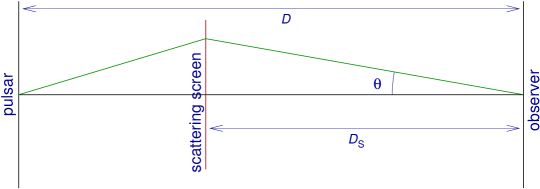
Figure 1: Interstellar scattering geometry. A particular sub-image is deflected by an apparent angle $\theta$.

As result of the effective deflection of the individual speckle, the geometrical path is increased, which results in a scattering delay (Fig. 1). This is similar to the situation in gravitational lensing, with the difference that in lensing the Shapiro (potential) delay contributes significantly to the total delay. In the case of interstellar scattering, the direct delay caused by the ISM is generally negligible.

For distances of the scattering medium and background source of $D_{\text{s}}$ and $D$, the delay for small deflections $\theta$ can be derived from the geometry in Fig. 1 as

$$\tau =\frac{1}{2}\theta^{2}D^{\prime}\quad\text{,} D^{\prime} =\frac{DD_{\text{s}}}{D-D_{\text{s}}}\quad\text{,}$$ (1)

where the effective distance $D^{\prime}$ is proportional to $D$ for a given $D_{\text{s}}/D$. For a canonical situation in which the scattering medium is in the middle between the background source and the observer ($D_{\text{s}}=D/2$), we have $D^{\prime}=D$.

Because different speckles have different deflections and delays, the signal is broadened angularly and temporally. The observed brightness depends on the relative phases of all speckles, which become decorrelated over bandwidths larger than the reciprocal scattering time. This scintillation can thus only be observed if the spectral resolution is finer than $1/\tau$.

For Kolmogorov turbulence, we expect and generally observe a wavelength dependence of

$$\theta\propto\lambda^{2.2}\quad\text{,}\qquad\tau\propto\lambda^{4.4}\quad\text{.}$$ (2)

This conference contribution is about utilising the relation $\tau\propto\theta^{2}$ not only for average scattering times $\tau$ and sizes $\theta$, but also for individual speckles within one source.

2 Scatter broadening in pulsars

The intrinsic sizes of pulsars are much smaller than their scattering sizes, so that the latter is not smeared out. In our study we use pulsars because of the unique feature to offer timing information in their radiation in the form of very regular and often narrow pulses. It is this feature that allows us to measure the scattering delays $\tau$ in a very direct way (Fig. 2).

Figure 2: Scatter-broadened profile of the pulsar B1815–15 at 1.4 GHz [1]. The intrinsic pulse-width is sufficiently small to reveal the exponential scattering tail that is expected for a thin scattering screen. This is also the target for which we show preliminary results in this contribution.

3 Comparing angular and temporal broadening

A comparison of characteristic scattering times $\tau$ and sizes $\theta$ can be used to determine the mean distance of the scattering screen(s) via Eq. (1). Fig. 3 shows this for a number of sources. This comparison does already provide interesting information, but it completely disregards the relation of $\tau$ vs. $\theta$ for different speckles in the same system. Because of this, it can, e.g., not distinguish between one scattering screen or many scattering screens with the same mean distance.

Figure 3: Comparison of measured scattering size (vertical axis) with temporal broadening, shown horizontally as predicted scattering size as derived from $\tau$ via the equivalent of Eq. (1) for a uniform distribution of scattering material [2, observations at 326 MHz]. The diagonal band marks equality within errors.

4 Secondary spectrum

An alternative way of studying the relation between $\tau$ and $\theta$ is provided by the secondary spectrum. To compute the secondary spectrum, one starts with the power in a dynamic spectrum (intensity as function of time and frequency) and then applies a second two-dimensional Fourier transform that converts the frequency axis into a delay axis and the time axis into a fringe-frequency axis (Fig. 4).

The delay corresponds to delays between different speckles, while the fringe-frequency measures the change with time due to proper motion (equivalent to a projected Doppler effect). The parabolic arcs (including the inverted arcs) that are generally seen in the secondary spectra can be explained as resulting from transverse motion (changing $\theta$) and the relation $\tau\propto\theta^{2}$. This approach provides a wealth of information, and can even be extended to interferometric observations [3]. However, it is model-dependent to some degree, because it uses the Doppler effect as proxy for $\theta$ and is only sensitive to a one-dimensional projection of $\theta$.

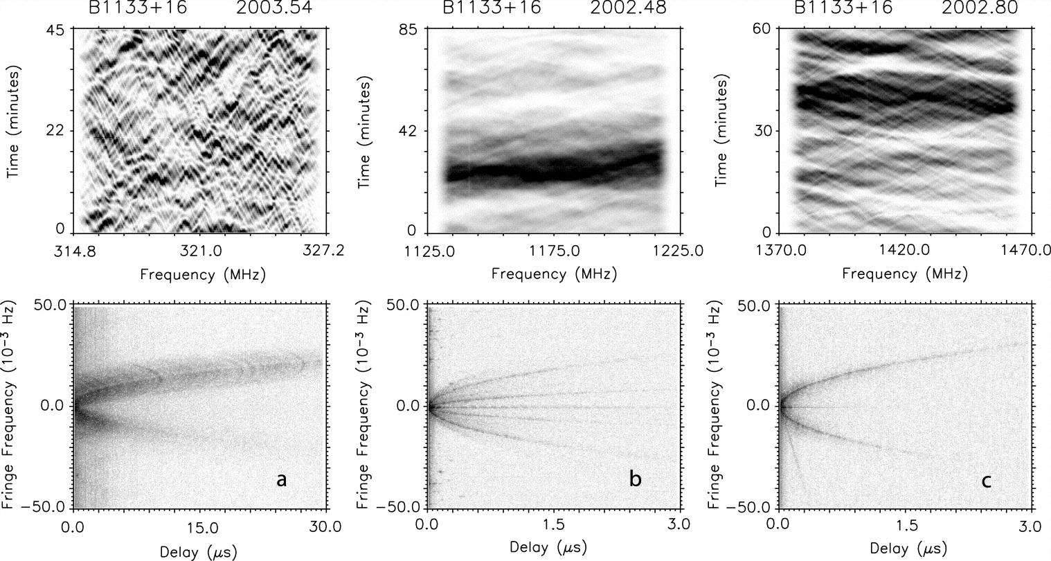
Figure 4: Dynamic spectra (top) and secondary spectra (bottom) for three pulsars [4]. The parabolas are an indirect result of the quadratic relation $\tau\propto\theta^{2}$.

5 Combined temporal and angular scattering study

Neither of the methods discussed so far utilise all the available information. The comparison of mean scattering times with sizes does not use the full profiles, while the secondary spectrum does not use the timing information provided by the pulsed emission. As one possible way of combining the advantages of both methods, we do not only want to study the temporal and spatial profiles independently but measure the signal strength as function of $\tau$ and $\theta$, where the deflection angle is even two-dimensional. The full three-dimensional profile can potentially provide much more information than the temporal and spatial profiles alone.

Fig. 5 shows expected profiles as function of $\tau$, $\theta$, and $\tau$ and $\theta$ combined, as well as expected visibility amplitudes. We immediately see that a combined measurement can distinguish between different distributions of scattering material even if the temporal and spatial profiles are almost unchanged.

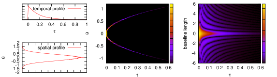
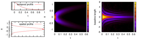
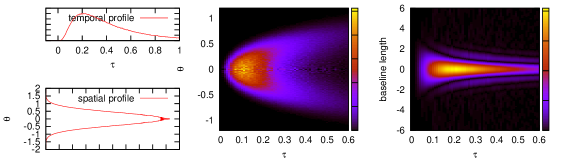
Figure 5: Simulated profiles for one screen (top), two screens (middle) and for a continuous scattering medium (bottom). Each panel shows the temporal and spatial profiles, the combined profile as function of $\tau$ and $\theta$ and the expected visibility amplitudes as function of $\tau$ and baseline length.

How can we measure the three-dimensional profile in practice? One option is to produce interferometric images as function of scattering delay $\tau$. In the case of a single scattering screen we expect to see a point that grows into an expanding ring, the radius of which goes with the square root of time (measured via apparent pulse phase). For several scattering screens or a continuous medium we would see an expanding fuzzy ring or blob instead. Alternatively, and more appropriate for sparse uv coverage, we can study the pulse profile as function of baseline length, where we would expect to see less scattered profiles on longer baselines.

6 Observations and analysis

We decided to observe eight bright pulsars with global VLBI at 1.4 GHz and 327/610 MHz. The targets were selected according to brightness and scattering parameters that allow us to resolve the temporal and angular scattering. This project (GW022A/B) was observed in June 2011 using the VLBA, five EVN stations and Arecibo. In the following we only discuss very preliminary results for the pulsar B1815–14 at 1.4 GHz. The baseband data were correlated in Bonn using DiFX (with incoherent de-dispersion) running on computer clusters at the MPIfR and AIfA. We first produced profiles from autocorrelations in order to create matched filters. These filters were then used for a gated correlation that was calibrated in AIPS. Amplitudes were taken from unscattered control pulsars, while the phases are determined from the targets. We then used these solutions to calibrate a third correlation that was binned into 400 slots per period. Images have not been produced yet, but (complex) profiles of calibrated visibilities.

Fig. 6 shows example profiles. We learn that the profiles on longer baselines are indeed less scattered. In addition, we already see that the angular scattering is inconsistent with growing Gaussians, because the baseline profiles have negative tails. These negative tails correspond to the negative visibilities expected for expanding rings.

A full quantitative analysis that can constrain the distribution of scattering material and measure its distance still has to be done.

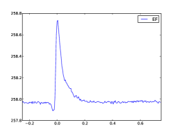
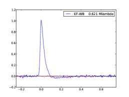
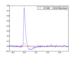
Figure 6: Pulse profiles in autocorrelation (EF, left) and in two baselines (centre and right, 0.621 k$\lambda$ and 0.918 k$\lambda$) for one scan of about 15 min. The real part is shown in solid blue, the imaginary part in dotted red. The negative pre-pulse dip in the left plot results from digitisation non-linearities and dispersion.

7 Outlook

There is a chance to improve the essential amplitude calibration by using information from the autocorrelations. In non-pulsar observations this is not possible, because the autocorrelations are generally dominated by system noise and not the target signal. For folded pulsar data, the noise can be subtracted easily, which opens this route for amplitude calibration. However, the data were digitised with 2 bits per sample, which introduces significant digitisation non-linearities. This can be taken into account, provided that the sampler statistics are known. In our case this is made more difficult by the switched power and (even more) by the pulse-calibration signals that distort the statistics on a 1 $\mu$sec period. This effect is most significant for Arecibo where the occupation numbers are completely skewed for certain pulse-cal period bins. Using an extended version of DiFX we are able to derive amplitudes with about 10 % accuracy, but this still has to be improved for the final calibration.

For some of the targets we will produce ‘movies’ as function of scattering delay that may show the expected expanding rings or blobs. The quantitative analysis will provide information about the distribution and distance of the scattering material in front of our target pulsars. Similar experiments are planned with LOFAR, which samples a different part of parameter space.

8 Acknowledgements

The author wants to thank Joris Verbiest (MPIfR) for providing the pulsar ephemerides.

References

- Löhmer et al. [2001] O. Löhmer, M. Kramer, D. Mitra, D. R. Lorimer, and A. G. Lyne. ApJ, 562:L157, 2001.
- Gwinn et al. [1993] C. R. Gwinn, N. Bartel, and J. M. Cordes. Astrophys. J. missing (missing) missing, 410:673, 1993.
- Brisken et al. [2010] W. F. Brisken et al. Astrophys. J. missing (missing) missing, 708:232, 2010.
- Cordes et al. [2006] J. M. Cordes, B. J. Rickett, D. R. Stinebring, and W. A. Coles. Astrophys. J. missing (missing) missing, 637:346, 2006.