Thermal Width of Quarkonium from Holography
Kazem Bitaghsir Fadafan, Seyed Kamal Tabatabaei

Physics Department, Shahrood University, Shahrood, Iran

From the AdS/CFT correspondence, the effects of charge and finite ’t Hooft coupling correction on the thermal width of a heavy quarkonium are investigated. To study the charge effect, we consider Maxwell charge which is interpreted as quark medium. In the case of finite ’t Hooft coupling corrections, $\mathcal{R}^{4}$ terms and Gauss-Bonnet gravity have been considered, respectively. It is shown that these corrections affect the thermal width. It is also argued that by decreasing the ’t Hooft coupling, the thermal width becomes effectively smaller. Interestingly, this is similar to analogous calculations in weakly coupled plasma.

1 Introduction

The experiments of Relativistic Heavy Ion Collisions (RHIC) have produced a strongly coupled quark$-$gluon plasma (QGP)(see review [1]). At a qualitative level, the data indicate that the QGP produced at the LHC is comparably strongly coupled and it is expected to be better approximated as conformal than is the case at RHIC [2]. There are no known quantitative methods to study strong coupling phenomena in QCD which are not visible in perturbation theory (except by lattice simulations). A new method for studying different aspects of QGP is the $AdS/CFT$ correspondence [1, 3, 4, 5, 6]. This method has yielded many important insights into the dynamics of strongly coupled gauge theories. It has been used to study hydrodynamical transport quantities at equilibrium and real time process in non-equilibrium [7]. Methods based on $AdS/CFT$ relate gravity in $AdS_{5}$ space to the conformal field theory on the four-dimensional boundary [5]. It was shown that an $AdS$ space with a black brane is dual to a conformal field theory at finite temperature [6].

In heavy ion collisions at the LHC, heavy quark related observables are becoming increasingly important [8]. In these collisions, one of the main experimental signatures of QGP formation is melting of quarkonium systems, like $J/\psi$ and excited states, in the medium [9]. They are also useful probes for QCD phenomenology [10]. The thermal width of these systems is an important subject in QGP [11]. This quantity emerges from the imaginary part of the heavy quark potential, which is related to quarkonium decay processes in the QGP [12]. In the effective field theory framework, thermal decay widths have been studied in [13, 14]. It was shown that at leading order, two different mechanisms contribute to the decay width, namely Landau damping and singlet-to-octet thermal breakup. As long as the Debye screening mass is larger than the binding energy, the former mechanism dominates over the latter. Also from the elementary process point of view, the Landau-damping mechanism corresponds to dissociation by inelastic parton scattering and the singlet-to-octet thermal breakup corresponds to gluon dissociation [15]. Beyond leading order, these two mechanisms would be the same.

The analytic estimate of the imaginary part of the binding energy and the resultant decay width were studied in [16]. The peak position and its width in the spectral function of heavy quarkonium can be translated into the real and imaginary part of the potential [17]. Using the soft-wall AdS/QCD model the finite-temperature effects on the spectral function in the vector channel have been studied and a similar behavior to lattice QCD results was found for the in-medium mass shift and the width broadening of the vector meson [18].

The effect of the imaginary part of the potential on the thermal widths of the states in both isotropic and anisotropic plasmas has been studied in [19, 20]. This study has been done by considering the modifications to the Coulombic wave function of the imaginary part of the potential for $J/\psi,\Upsilon$ and $\chi_{b}$ for both an isotropic and anisotropic QGP. The expectation value of the imaginary part of the quarkonium potential gives the thermal width, which was obtained analytically in the case of an isotropic plasma in [16]. For the case of $\Upsilon$ it is on the order of 20-100 MeV, which is comparable to the decay width of $\Upsilon\rightarrow e^{+}e^{-}$.

The thermal width of heavy quarkonium in a hot strongly coupled isotropic plasma was, from a holographic point of view, initially studied in [21]. In this approach, the thermal width of heavy quarkonium states originates from the effect of thermal fluctuations due to the interactions between the heavy quarks and the strongly coupled medium. This is described holographically by integrating out thermal long wavelength fluctuations in the path integral of the Nambu-Goto action in a curved background spacetime. This study was extended to the case of anisotropic plasma in [22, 23] and imaginary potential formula in a general curved background was obtained. It was also shown that the thermal width is decreased in the presence of anisotropy and a larger decrease happens along the transverse plane. This method was revisited in [24] and general conditions for the existence of an imaginary part for the heavy quark potential were obtained. In the context of AdS/CFT, there are other approaches which can lead to a complex static potential [26, 27]. In [26], the extended range of the radial distance $u$ was studied in such a way that the string world-sheet solutions of the Wilson loop corresponding to the static, potential become complex, and therefore the corresponding static potential develops an imaginary part. The method in [27] is based on the spectral decomposition of the Euclidean Wilson loop and its analytic continuation to the real time. The imaginary potential in this method grows linearly with temperature, which is qualitatively consistent with that obtained in [21, 26].

In this paper, we study different effects on the thermal width by considering the effects of the charge and the finite ’t Hooft coupling correction on the hot plasma. To study the charge effect, we consider a Maxwell charge which can be interpreted as a quark medium. Therefore on the gravity side, we consider the non-extremal Reissner-Nordstrom AdS $(RNAdS)$ black hole. The finite ’t Hooft coupling corrections also correspond to $\mathcal{R}^{4}$ corrections and Gauss-Bonnet terms, respectively. An understanding of how the imaginary part of the potential and thermal width of heavy quarkonium are affected by these corrections may be essential for theoretical predictions.

Melting of a heavy meson like $J/\psi$ and excited states like $\chi_{c}$ and $\psi^{\prime}$ in the quark medium have been investigated in [47]. It was shown that the excited states melt at higher temperatures. Heavy quarks in the presence of higher derivative corrections have been studied in [31, 32]. Now we continue with considering these effects on the thermal width of quarkonium.

This paper is organized as follows. In the next section, we will present an example for the connection between the imaginary part of the potential and confinement. This example confirms that the imaginary potential is zero in the confinement phase. We give the general expressions to study the thermal width in section 3. Also in this section, we use the general formulas and investigate the thermal width behavior at finite coupling and in the presence of a dense medium. In the last section we summarize our results.

2 Imaginary potential and confinement

As was argued in [24], the presence of a black brane is necessary in order to have a non-zero imaginary potential. In other words, in the absence of a black brane the imaginary part of the potential vanishes. In this section, we examine this idea in a theory which exhibits a confinement-deconfinement transition at some finite temperature $T_{c}$. We are not going to carry out the details of the calculations which prove that the imaginary part of the potential is zero in the confined phase.

One may consider the confining SU(N) gauge theory based on N D4 branes on a circle. In particular, fundamental parameters are an energy scale in addition to temperature. The vacuum of the theory at zero temperature confines the color charge. One expects that the imaginary potential in the low T phase should vanish.

The model that we consider is the model of Witten [6] which is based on N D4 branes wrapped on a circle. In this theory the field theory is a non-supersymmetric SU(N) Yang-Mills theory that confines at low temperatures [6]. Although the theory is different from pure Yang-Mills theory, it exhibits linear confinement of the quarks in vacuum. The gravitational background dual to the vacuum is known analytically to be

$$ds^{2} = (\frac{u}{l})^{3/2}\left(-dt^{2}+d\rho^{2}+\rho^{2}d\phi^{2}+dx_{3}^{2}+f(u)dx_{4}^{2}\right)+(\frac{l}{u})^{3/2}\left(\frac{du^{2}}{f(u)}+u^{2}d\Omega_{4}^{2}\right)$$ (2.1)

$$F_{(4)}=\frac{2\pi N}{V_{4}}\epsilon_{4},\,\,\,\,\,e^{\phi}=g_{s}(\frac{u}{l})^{3/4},\,\,\,\,l^{3}=\pi g_{s}N_{c}l_{s}^{3}.$$

A typical length scale associated to the D4 brane geometry is $l$ which all dimensionful quantities measure in units of $l$. The volume of the unit $S^{4}$ and the associated volume form are $V_{4}$ and $\epsilon_{4}$, respectively. Also

$$f(u)=1-(\frac{u_{k}}{u})^{3},\,\,\,\,\,\frac{u_{k}}{l}=\frac{4l^{2}}{9R^{2}}.$$ (2.2)

The latter equation follows from demanding the absence of a conical singularity at the tip of the cigar $u_{k}$ that is spanned by $x_{4}$ and $u$. At the high temperature phase, the black hole geometry is given by

$$ds^{2} = (\frac{u}{l})^{3/2}\left(-F(u)dt^{2}+d\rho^{2}+\rho^{2}d\phi^{2}+dx_{3}^{2}+dx_{4}^{2}\right)+(\frac{l}{u})^{3/2}\left(\frac{du^{2}}{F(u)}+u^{2}d\Omega_{4}^{2}\right).$$ (2.3)

Here the blackness function $F(u)$ and the temperature are

$$F(u)=1-(\frac{u_{h}}{u})^{3},\,\,\,\,\,\frac{u_{h}}{l}=\frac{16\pi^{2}l^{2}}{9}T^{2}.$$ (2.4)

There is a critical temperature $T_{c}=\frac{1}{2\pi R}$ where the theory is confined for $T<T_{c}$ and the geometry is described by (2.1), whereas, for $T>T_{c}$ the theory is deconfined and is given by (2.3). The ratio of $\frac{u_{h}}{u_{k}}$ is given by

$$\frac{u_{h}}{u_{k}}=\left(\frac{T}{T_{c}}\right)^{2}.$$ (2.5)

Based on the results of [24], If $u_{k}>u_{h}$ then the U-shaped string cannot go past $u_{k}$ and one cannot consider fluctuations beyond $u_{k}$. From AdS/CFT, one may interpret this condition from (2.5) in terms of the temperature. Then, more explicitly, for $T<T_{c}$ the imaginary potential vanishes, while for $T>T_{c}$ it is not zero. As a result, in this geometry, which shows the confinement-deconfinement transition at $T_{c}$, the imaginary potential is zero in the confinement phase.

3 Thermal width from holography

In order to compute thermal widths from holography, one should consider a heavy quark anti-quark pair in the boundary of a black hole geometry. In this section, we give the general formulas for calculating the distance between the quark and the antiquark, $L$, the real part of the potential $ReV_{Q\bar{Q}}$ and the imaginary part of the potential $\text{Im}V_{Q\bar{Q}}$ in terms of the geometry coordinates.

We consider the general gravity as follows:

$$ds^{2}=G_{tt}dt^{2}+G_{xx}dx_{i}^{2}+G_{uu}du^{2},$$ (3.1)

here the metric elements are functions of the radial distance $u$ and $x_{i}=x,y,z$ are the boundary coordinates. In these coordinates, the boundary is located at infinity. We study a static quark antiquark system at the boundary as an open string in the bulk space from the gauge string duality point of view [25]. Using the usual orthogonal Wilson loop which corresponds to the heavy QQ̄ pair, and assuming the system to be aligned in the $x$ direction

$$t=\tau,\quad x=\sigma,\quad u=u(\sigma),$$ (3.2)

one finds the following generic formulas for the heavy meson. In these formulas $u_{*}\equiv u(x=0)$ is the deepest point of the U-shaped string. The metric functions appear as $V(u)\equiv-G_{tt}G_{xx}$ and $W(u)\equiv-G_{tt}G_{uu}$.

• The distance between quark and antiquark, $L$ is given by

  $$L=2\,\int_{u_{*}}^{\infty}du~{}\left[\frac{V(u)}{W(u)}\left(\frac{V(u)}{V(u_{*})}-1\right)\right]^{-\frac{1}{2}}~{}~{},$$ (3.3)

• The real part of heavy quark potential, $ReV_{Q\bar{Q}}$ is as follows:

  $$ReV_{Q\bar{Q}}=\frac{1}{\pi\alpha^{\prime}}\left[\int_{u_{*}}^{\infty}du~{}\left(\left(\frac{1}{W(u)}-\frac{V(u_{*})}{V(u)W(u)}\right)^{-1/2}-\sqrt{W_{0}(u)}\right)-\int_{0}^{u_{*}}du~{}\sqrt{W_{0}(u)}\right],$$

  (3.4)

  here $W_{0}(u)=W(u\rightarrow\infty)$.

• The imaginary part of the potential is negative and it is given by

  $$\text{Im}V_{Q\bar{Q}}=-\frac{1}{2\sqrt{2}\alpha^{\prime}}\left[\frac{V^{\prime}(u_{*})}{2V^{\prime\prime}(u_{*})}-\frac{V(u_{*})}{V^{\prime}(u_{*})}\right]~{}\sqrt{W(u_{*})}~{}.$$ (3.5)

  The derivatives are with respect to $u$. For the special case of $W(u)=1$, this formula reduces to the case of an isotropic plasma [21], while $W(u)\neq 1$ corresponds to the anisotropic plasma [22, 23] .

These generic formulas give the related information of the heavy quarkonium in terms of the metric elements of a background (3.1).

To find the $\text{Im}V$, one should express it in terms of the length $L$ of the Wilson loop instead of $u_{*}$ using the equation (3.3). There is an important point for long U-shaped strings because it would be possible to add new configurations [28]. Here we are interested mostly in distances $LT<1$ and do not consider such configurations.

We use a first-order non-relativistic expansion,

$$\Gamma=-<\psi|\text{ImV}_{Q\bar{Q}}|\psi>,$$ (3.6)

to calculate the thermal width of a heavy quarkonium like $\Upsilon$ meson. The imaginary potential is given by (3.5); also $|\psi>$ is the Coulombic wave function of the Coulomb potential of the heavy quarkonium. From the holographic point of view, the potential between infinitely massive quarks in a pure AdS background is a Coulomb-like potential,

$$V_{Q\bar{Q}}(L)=-\frac{4\,\pi^{2}}{\Gamma(1/4)^{4}}\,\frac{\sqrt{\lambda}}{L}.$$ (3.7)

The original calculation of this result comes from considering the rectangular Wilson loop in the vacuum of strongly coupled N = 4 SYM theory [29]. The generalization to finite temperature has been done in [30]. The effect of higher derivative corrections on the real part of the potential within the gauge/gravity duality has been done in [31, 32] and it was found that the dissociation length becomes shorter with the increase of the coupling parameters of the higher curvature terms. The rotating heavy quarkonium also is studied in [33, 34, 35, 47].

Regarding the Coulombic potential in (3.7), applying a potential model may therefore provide qualitatively useful insight. We consider the ground-state wave function of $|\psi>$ in a Coulomb-like potential $V=-A/L$ where $A$ in the case of N=4 SYM comes from (3.7). In the ground state of the energy levels of a bound state of heavy quarks with mass of $m_{Q}$, the Bohr radius is defined as $a_{0}=2/m_{Q}A$. The wave function is

$$|\psi>=\frac{1}{\sqrt{\pi}a_{0}^{3/2}}\,e^{-L/a_{0}}.$$ (3.8)

By considering different effects on the plasma, the real part of the potential is not given by just the Coulombic term. But this term provides the leading contribution for the potential of heavy quarkonia; therefore, it justifies the use of a Coulomb-like wave function $|\psi>$ in (3.8) to determine the width. Considering a finite temperature plasma will not change the coefficient $A$ in the Coulombic potential. However, by studying the charge and finite coupling corrections one should modify $A$. We find the potential using the numerical fitting in this case. More details will be found in the next sections where we show the behavior of $\Gamma$ in terms of parameters of the plasma. As a result, by considering different effects on the plasma, we also find $A$ by fitting methods. This approach is carefully followed in [23].

To begin with, we calculate $\Gamma$ in the $N=4$ SYM. The metric functions are

$$V(u)=\frac{u^{4}-u_{h}^{4}}{R^{4}},\,\,\,\,\,W(u)=1.$$ (3.9)

where the horizon is located at $u_{h}$ and the temperature of the hot plasma is given by $u_{h}=\pi R^{2}T$. In this case we do not consider any correction and call imaginary potential as $\text{ImV}_{Q\bar{Q}}^{(0)}$. From (3.5) it is found to be

$$\text{ImV}_{Q\bar{Q}}^{(0)}=-\frac{\pi\sqrt{\lambda}\,T}{24\sqrt{2}}\,\left(\frac{3\xi^{4}-1}{\xi}\right),\,\,\,\,\,\,\,\xi=\frac{u_{h}}{u_{*}}.$$ (3.10)

The imaginary potential is negative; then it implies that there is a lower bound for the deepest point of the U-shaped string, i.e. $\xi_{min}=0.76$. This minimum value is found by solving $\text{ImV}_{Q\bar{Q}}^{(0)}=0$. The maximum value $\xi_{max}$ occurs when the distance $L$ approaches the maximum value. In the left plot of Fig. 1, we show explicitly these values with a gray filled line.

  

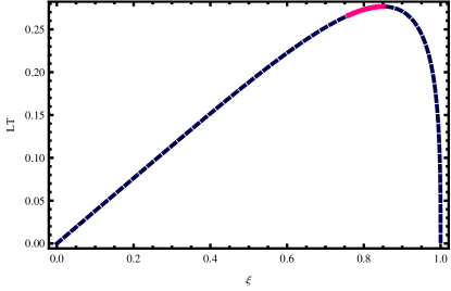
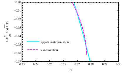
Figure 1: Left: The distance between quark antiquark versus the $\xi$. The specified region in this plot correspond to the valid region for studying the imaginary potential. Right: The imaginary potential for the accepted values of $\xi$ or $L$ in the specified region of right plot.

The imaginary potential for these values of $\xi$ is plotted in the right plot of Fig.1. It is clearly seen that the imaginary potential starts to be generated at $L_{min}$ or $\xi_{min}$ and increases in absolute value with $L$ until a value $L_{max}$ or $\xi_{max}$. It should be noticed that for $\xi$ very close to the horizon one should consider higher order corrections [28].

By finding the imaginary potential, the thermal width also is found from (3.6) as

$$\Gamma=-\frac{4}{a_{0}^{3}}\int_{0}^{\infty}L^{2}dLe^{-2L/a_{0}}\text{ImV}_{Q\bar{Q}}.$$ (3.11)

There is a limitation to the calculation of the thermal width from holography [23]. One finds from Fig. 1 that the imaginary potential is well defined for a separation in $(L_{min}~{},~{}L_{max})$. On the other hand, from a physical point of view we expect that the imaginary potential should exist also for a larger separation. One may fix this limitation by assuming that a solution would be exist at larger distances. We find this solution by an extrapolating approach. Therefore, we extend the solution in the $(L_{min}~{},~{}L_{max})$ region to larger distances by extrapolating the curve. This is the reason why we fitted the straight line in the right plot of Fig. 1 which covers larger distances to infinity.

Briefly, we do the integration in (3.6) in $(L_{min}~{},~{}L_{max})$ and then we compute the width in the region $(L_{min}~{},~{}\infty)$ by using a reasonable extrapolation for imaginary potential. It should be noticed that in [21], the integration in (3.6) has been done in $(0~{},~{}\infty)$ and straight line fitting was used for $L<L_{min}$ region. We do not follow this approach because the imaginary potential is not defined in $(0~{},~{}L_{min})$. As a result, in our approach, the value of the width is two orders of magnitude smaller than the result in [21]. The width in dependence on use of the extrapolation method has been discussed also in [24].

We call the width as $\Gamma^{(0)}$. One finds that for $\Upsilon$ with parameters as $m_{Q}=4.7GeV,\lambda=9,R=1$ and at $T=0.3GeV$ the width is $\Gamma^{(0)}=.487MeV$. In the next sections we will normalize the thermal widths in the presence of corrections to the $\Gamma^{(0)}$ value.

3.1 Thermal width at finite coupling

From the AdS/CFT, the coupling which is denoted as ’t Hooft coupling $\lambda$ is related to the curvature radius of the $AdS_{5}$ and $S_{5}$ $(R)$, and the string tension $(\frac{1}{2\pi\alpha^{\prime}})$ by $\sqrt{\lambda}=\frac{R^{2}}{\alpha^{\prime}}$. A general result of the AdS/CFT correspondence states that the effects of finite but large $\lambda$ coupling in the boundary field theory are captured by adding higher derivative interactions in the corresponding gravitational action. In our study, the corrections to the AdS-Schwarzschild black brane that will be considered are $\mathcal{R}^{4}$ and $\mathcal{R}^{2}$ corrections. The thermal width in these cases is called $\Gamma^{(\lambda)}$ and $\Gamma^{(\lambda_{GB})}$, respectively.

• $\mathcal{R}^{4}$ corrections:

Since the $AdS/CFT$ correspondence refers to the complete string theory, one should consider the string corrections to the 10D supergravity action. The first correction occurs at order $(\alpha^{\prime})^{3}$ [37]. In the extremal $AdS_{5}\times S^{5}$ it is clear that the metric does not change [38], conversely this is no longer true in the non-extremal case. Corrections in inverse ’t Hooft coupling $1/\lambda$ which correspond to $\alpha^{\prime}$ corrections on the string theory side, were found in [37]. The functions of the $\alpha^{\prime}$-corrected metric are given by [39]

$$G_{tt} = -u^{2}(1-w^{-4})T(w),$$

$$G_{xx} = u^{2}X(w),$$

$$G_{uu} = u^{-2}(1-w^{-4})^{-1}U(w),$$ (3.12)

where

$$T(w) = 1-k\bigg{(}75w^{-4}+\frac{1225}{16}w^{-8}-\frac{695}{16}w^{-12}\bigg{)}+\dots,$$

$$X(w) = 1-\frac{25k}{16}w^{-8}(1+w^{-4})+\dots,$$

$$U(w) = 1+k\bigg{(}75w^{-4}+\frac{1175}{16}w^{-8}-\frac{4585}{16}w^{-12}\bigg{)}+\dots,\$$ (3.13)

and $w=\frac{u}{u_{h}}$. As before, there is an event horizon at $u=u_{h}$ and the geometry is asymptotically $AdS$ at large $u$ with a radius of curvature $R=1$. The expansion parameter $k$ can be expressed in terms of the inverse ’t Hooft coupling as

$$k=\frac{\zeta(3)}{8}\lambda^{-3/2}\sim 0.15\lambda^{-3/2}.$$ (3.14)

The temperature is given by

$$T=\frac{u_{h}}{\pi R^{2}(1-k)}.$$ (3.15)

 

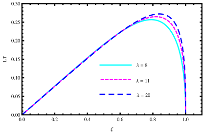
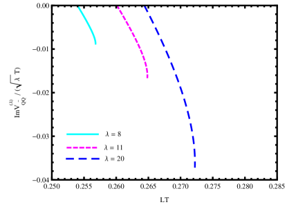
Figure 2: Left: The distance between quark-antiquark versus the $\xi$ for different values of coupling $\lambda$. From top to down $\lambda$= 20, 11, 8. Right: The imaginary potential for $\lambda$=8,11,20 from left to right.

The imaginary potential is found analytically (3.5). However, in this case it is a lengthy equation. We expand the result in terms of the expansion parameter $k$ as follows:

$$\text{ImV}_{Q\bar{Q}}^{(\lambda)}=\text{ImV}_{Q\bar{Q}}^{(0)}+k\,\frac{\pi T\sqrt{\lambda}}{1152\sqrt{2}}\,g(\xi)+O(k^{2})$$ (3.16)

where $g(\xi)=\left(-48-10656\xi^{4}-1775\xi^{8}+138840\xi^{12}-105495\xi^{16}+18090\xi^{20}\right)/\xi$. The first term is the imaginary potential in (3.10).

To find $\Gamma^{(\lambda)}$, we study behavior of the quark-antiquark distance in terms of $\xi$ for different values of $\lambda$. As shown in the left plot of Fig. 2 by increasing the coupling constant the maximum value of $L$ increases. In the right plot of this figure we show effect of coupling on the imaginary potential. One finds that by increasing the coupling, $L_{min}$ also increases. As an example, by choosing $R=1$, $T=0.3GeV$ and for $\lambda=8,11,20$, we find $L_{min}T\simeq 0.254,0.260,0.264$ and $L_{max}T\simeq 0.257,0.265,0.272$. We conclude that the imaginary part of the potential in the presence of coupling corrections is generated for larger distances:

$$L_{min}^{\lambda_{1}}<L_{min}^{\lambda_{2}}<L_{min}^{\infty}.$$ (3.17)

where $\lambda_{1}<\lambda_{2}<\infty$. Therefore, we find that in absolute value the imaginary potential is increased due to finite coupling corrections.

It would be important to notice that we cannot use the extrapolation method in this case. This is so because the sign of the imaginary potential for $\xi>\xi_{max}$ is not always negative and changes. Then we cannot use a straight line approximation to consider the larger values of $L$ like we did in the right plot of Fig. 1. Using this point we integrate the thermal width $\Gamma^{(\lambda)}$ from $L_{min}$ to $L_{max}$. We show $\Gamma^{(\lambda)}$ relative to the $\Gamma^{(0)}$ in this interval in Fig. 3. We used the gauge theory coupling $\lambda=100$ in this case to calculate $\Gamma^{(0)}$. As is clear from this figure, when $\lambda$ goes to infinity $\frac{\Gamma^{(\lambda)}}{\Gamma^{(0)}}$ goes to unity. The maximum value of $\frac{\Gamma^{(\lambda)}}{\Gamma^{(0)}}$ equals to $5.22$, which occurs at $\lambda_{c}=28$.

At strong coupling, an estimate of how the thermal width of heavy quarkonium changes with the shear viscosity to entropy density ratio, $\eta/s$, is studied in [24]. It is found that in the presence of curvature-squared corrections like Gauss-Bonnet terms, the thermal width as a function of $\eta/s$ decreases. It has been shown that considering $\mathcal{R}^{4}$ corrections increases $\eta/s$ [40]. One concludes that decreasing $\lambda$ leads to increasing $\eta/s$. Now, one finds from Fig. 3 that by decreasing $\lambda$ from $\lambda_{c}$, which means increasing $\eta/s$, the width becomes effectively smaller. Interestingly this is similar to analogous calculations in perturbative QCD [11]. In this study, it was argued that at strong coupling for a quarkonium with a very heavy constituent mass, the thermal width can be ignored [11] which is in good agreement with our result.

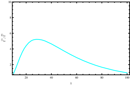
Figure 3: The thermal width versus the finite coupling correction computed by considering $\mathcal{R}^{4}$ corrections. We used the gauge theory coupling $\lambda=100$ in this case.

• $\mathcal{R}^{2}$ corrections:

Next, we study $\mathcal{R}^{2}$ corrections to the thermal width which is called $\Gamma^{(\lambda_{GB})}$.

In five dimensions, we consider the theory of gravity with quadratic powers of curvature as Gauss-Bonnet(GB) theory. The exact solutions and thermodynamic properties of the black brane in GB gravity are discussed in [41, 42, 43]. The metric functions are given by

$$G_{tt}=-N\,u^{2}\,h(u),\,\,\,\,\,\,G_{uu}=\frac{1}{u^{2}h(u)},\,\,\,\,\,G_{xx}=G_{yy}=G_{zz}=u^{2},$$ (3.18)

where

$$h(u)=\frac{1}{2\lambda_{GB}}\left[1-\sqrt{1-4\lambda_{GB}\left(1-\frac{u_{h}^{4}}{u^{4}}\right)}\right].$$ (3.19)

In (3.18), $N=\frac{1}{2}\left(1+\sqrt{1-4\lambda_{GB}}\right)$ which is an arbitrary constant that specifies the speed of light of the boundary gauge theory and we choose it to be unity. Beyond $\lambda_{GB}<1/4$ there is no vacuum AdS solution and one cannot have a conformal field theory at the boundary. Causality leads to new bounds for the value of the Gauss-Bonnet coupling constant as follows: $-7/36<\lambda_{GB}<9/100$ [44]. The temperature also is given by

$$T=\sqrt{N}\,\frac{u_{h}}{\pi R^{2}}.$$ (3.20)

Also, the ’t Hooft coupling of the dual strongly coupled CFT is $\lambda=\frac{N^{2}R^{4}}{\alpha^{\prime 2}}$ .

  

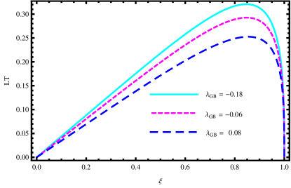
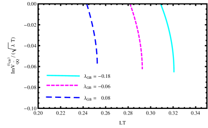
Figure 4: Left: The distance between quark-antiquark versus the $\xi$ for different values of Gauss-Bonnet coupling $\lambda_{GB}$. From top to down $\lambda_{GB}$=-0.18, -0.06, 0.08. Right: the imaginary potential versus the Gauss-Bonnet coupling constant. From right to left $\lambda_{GB}$=-0.18, -0.06, 0.08.

The thermal width in this background has been studied in [24]. Also the behavior of the width in terms of the shear viscosity to entropy density ratio was found. Here, we present further details and express the final results in terms of the Gauss-Bonnet coupling constant. As it was pointed out, our extrapolation method is different from [24].

The behavior of $L$ in terms of $\xi$ for different values of $\lambda_{GB}$ is shown in Fig. 4. It is clearly seen in the left plot of Fig. 4 that by increasing the coupling constant the maximum value of $L$ decreases. This behavior is not the same as the $\mathcal{R}^{4}$ corrections in Fig.2.

The imaginary potential in the Gauss-Bonnet gravity results from (3.5). The result can be expressed as follows:

$$\text{ImV}_{Q\bar{Q}}^{(\lambda_{GB})}=-\frac{h\pi T\sqrt{\lambda}}{4\sqrt{2}N\xi}$$ (3.21)

$$\frac{1-h+\left(-8+6h+(9-7h)\xi^{4}\right)\lambda_{\text{GB}}+4\left(4-2h+(-9+5h)\xi^{4}+3\xi^{8}\right)\lambda_{\text{GB}}^{2}}{\left(1-h+2\left(-2+\xi^{4}\right)\lambda_{\text{GB}}\right)\left(3-3h-6\left(4-2h+(-3+2h)\xi^{4}\right)\lambda_{\text{GB}}+8\left(6-9\xi^{4}+\xi^{8}\right)\lambda_{\text{GB}}^{2}\right)},$$

where

$$h=\sqrt{1+4\left(-1+\xi^{4}\right)\text{$\lambda_{GB}$}}.$$ (3.22)

In the right plot of this figure we show effect of coupling on the imaginary potential. For example, by choosing $R=1$, $T=0.3GeV$, $\lambda=9$ and for $\lambda_{GB}=-0.18,-0.06,0.08$, we find $L_{min}T\simeq 0.30,0.28,0.24$ and $L_{max}T\simeq 0.32,0.29,0.25$. Comparing with $\mathcal{R}^{4}$ corrections, one finds different behavior, i.e. by increasing the coupling $L_{min}$ decreases. This means that the imaginary potential in the Gauss-Bonnet gravity starts to be generated for smaller distances. We find that the absolute value of the imaginary part of the potential is increased due to finite coupling corrections.

In this case also we should do the integration in (3.11) in $(L_{min}~{},~{}L_{max})$ and one cannot consider larger lengths by extrapolating the curves in Fig.4. We would like to emphasize that using this method leads to the Fig.5. The modifications due to the finite coupling corrections to the Coulombic part of the real potential have been considered, too. At $\lambda_{GB}=-0.06$, there is a maximum value for $\Gamma^{(GB)}/\Gamma^{(0)}$ which is $1.004$. For other values of the coupling constant, the thermal width decreases.

3.2 Medium effect on the thermal width

In this section, we consider the quarkonium in the medium composed of light quarks and gluons [45]. It is shown that at the high temperature, the gravity dual to the QGP phase is the Reissner-Nordstrom AdS $(RNAdS)$ black hole and at the low temperature, the dual geometry to the hadronic phase is the thermal charged AdS $(tcAdS)$ space. The confinement/deconfinement phase transition in the quark medium is discussed in [45] and an influence of matters on the deconfinement temperature, $T_{c}$, is investigated. Using a different normalization for the bulk gauge field, it is shown that the critical baryonic chemical potential becomes $1100MeV$ which is comparable to the QCD result [46]. Melting of a heavy meson is investigated in [47] and it is found that the melting mechanism in the QGP and in the hadronic phase are the same, i.e. the interaction between heavy quarks is screened by the light quarks. The drag force on a moving heavy quark and the jet quenching parameter in the background of RNAdS black hole are studied in [48].

,

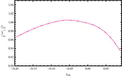
Figure 5: The normalized thermal width versus the Gauss-Bonnet coupling correction. There is a maximum value at $\lambda_{GB}=-0.06$.

Before calculating the thermal width, we will give a brief review of [45]. In this background the density in the dual field theory is mapped to a bulk gauge field. The Euclidean action describing the five-dimensional asymptotic $AdS$ space with the gauge field is given by

$$S=\int d^{5}x\sqrt{G}\left(\frac{1}{2\kappa^{2}}\left(-{\cal R}+2\Lambda\right)+\frac{1}{4g^{2}}F_{MN}F^{MN}\right).$$ (3.23)

Here $\kappa^{2}$ is proportional to the five-dimensional Newton constant and $g^{2}$ is a five-dimensional gauge coupling constant. The cosmological constant is given by $\Lambda=\frac{-6}{R^{2}}$, where $R$ is the radius of the $AdS$ space.

As it was pointed out the QGP and hadronic phases are described by the $tcAdS$ and the $RNAdS$ black hole, respectively [46]. It was argued in section 2 that the imaginary part of the potential in the confinement phase would be zero, then we focus on the QGP phase. This solution is considered as follows:

$$ds^{2}=R^{2}u^{2}\left(-f(u)dt^{2}+d\vec{x}^{2}+\frac{1}{u^{4}f(u)}du^{2}\right),$$ (3.24)

where the blackness function $f(u)$ is given by

$$f(u)=1-mu^{-4}+q^{2}u^{-6}.$$ (3.25)

In these coordinates, $u$ denotes the radial coordinate of the black hole geometry and $t,\vec{x}$ label the directions along the boundary at the spatial infinity. The boundary is located at infinity and the geometry is asymptotically $AdS$ with radius $R$. The event horizon is located at $f(u_{h})=0$ where $u_{h}$ is the largest root of this equation. The black hole mass $(m)$ and the temperature $(T)$ are given by

$$m=u_{h}^{4}+q^{2}u_{h}^{-2},\,\,\,\,\,\,T=\frac{u_{h}}{\pi}\left(1-\frac{q^{2}}{2u_{h}^{6}}\right).$$ (3.26)

where $q$ is the black hole charge.

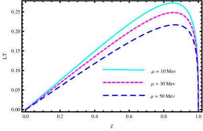
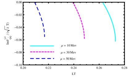
Figure 6: Left: The distance between quark-antiquark versus the $\xi$ for different values of chemical potential $\mu$. From top to down $\mu$=10MeV, 30MeV, 50MeV .Right: The imaginary potential versus the $L$ for $\mu$=10MeV, 30MeV, 50MeV .

The time-component of the bulk gauge field is $A_{t}(u)=i(2\pi^{2}\mu-Q\,u^{-2})$ where $\mu$ and $Q$ are related to the chemical potential and quark number density in the dual gauge theory. Regarding the Drichlet boundary condition at the horizon, $A_{t}(u_{h})=0$, one finds $Q=2\pi^{2}\mu\,u_{h}$. The black hole charge $q$ and the quark number density $Q$ are also related to each other by this equation

$$Q=\sqrt{\frac{3}{2n}}\,q.$$ (3.27)

where $n^{-1}=\frac{g^{2}R^{2}}{\kappa^{2}}$ is the color number.

Now using the general results in (3.4) and (3.4), we study the behavior of $L$ in terms of $\xi$ for different values of $\mu$. The results are shown in Fig. 6. It is clearly seen in the left plot of this figure that by increasing the chemical potential the maximum value of $L$ decreases. On the contrary, considering $\mathcal{R}^{4}$ corrections increases the maximum value of $L$ which can be seen in Fig. 2.

The imaginary potential in this background is found from (3.5). The result is expressed as follows:

$$\text{ImV}_{Q\bar{Q}}^{(\mu)}=\frac{\sqrt{\lambda}u_{h}\left(32n^{2}\pi^{8}\mu^{4}\xi^{10}\left(3-2\xi^{2}\right)+12n\pi^{4}\mu^{2}\xi^{4}\left(6-13\xi^{2}+3\xi^{6}\right)u_{h}^{2}+9\left(-1+3\xi^{4}\right)u_{h}^{4}\right)}{24\sqrt{2}\left(16n^{2}\pi^{8}\mu^{4}\xi^{13}-9\xi u_{h}^{4}\right)}.$$ (3.28)

Here at $\mu=0$, one finds the exact result in (3.10).

In the right plot of Fig. 6, we show effect of chemical potential on the imaginary potential. We fixed the parameters as $R=1$, $\lambda=9$, $T=0.3GeV$ and $n=1$. For $\mu=10MeV,30MeV$ and $\mu=50MeV$, one finds $L_{min}T\simeq 0.26,0.23,0.20$ and $L_{max}T\simeq 0.27,0.24,0.21$. Comparing with $\mathcal{R}^{4}$ corrections, one finds different behavior, i.e. by increasing the chemical potential $L_{min}$ decreases:

$$L_{min}^{\mu_{1}}<L_{min}^{\mu_{2}}<L_{min}^{\mu_{3}}$$ (3.29)

where $\mu_{1}>\mu_{2}>\mu_{3}$. As a result, one concludes that the imaginary potential in the presence of light quarks starts to be generated for smaller distances, while at finite $\lambda$ coupling it starts at a larger distance.

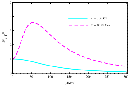
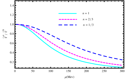
Figure 7: Thermal width in the presence of light quarks. Left: The ratio of $\frac{\Gamma^{(\mu)}}{\Gamma^{(0)}}$ is shown versus the chemical potential. Two different temperatures from top to down are $T=0.122GeV$ and $T=0.3GeV$. Right: The effect of increasing flavor color number on the ratio of $\frac{\Gamma^{(\mu)}}{\Gamma^{(0)}}$ at $T=0.3GeV$.

To calculate the thermal width, one should do the integration in (3.11) in $(L_{min}~{},~{}L_{max})$. It is found that by increasing the temperature, $\Gamma^{(\mu)}$ also increases. At fixed temperature, there is a maximum value for $\Gamma^{(\mu)}$. The ratio of $\frac{\Gamma^{(\mu)}}{\Gamma^{(0)}}$ versus the chemical potential is shown in the Fig. 7. In this figure, two different temperatures from top to down are $T=0.122GeV$ and $T=0.3GeV$, respectively.

We introduce $N_{f}=nN_{c}$ where $N_{f}$ and $N_{c}$ are the number of flavors and color fields, respectively. Now one can find the behavior of the thermal width when the flavor number of quarks increases. In the right plot of Fig.7, the effect of increasing flavor color number on the ratio of $\frac{\Gamma^{(\mu)}}{\Gamma^{(0)}}$ has been shown at $T=0.3GeV$. It is seen that the maximum value of thermal width does not change but the rate of it versus the chemical potential changes, monotonically.

4 Conclusion

In this paper, we studied the different effects on the thermal width from holography. We considered the effects of the charge and the finite ’t Hooft coupling correction on the hot plasma. An understanding of how the width changes by these corrections may be essential for theoretical predictions in perturbative QCD [36, 15]. To study the charge effect, we considered the Maxwell charge, which is interpreted as a quark medium. The effects of finite but large couplings are considered by adding higher derivative corrections in the gravity background. Especially, $\mathcal{R}^{4}$ terms and Gauss-Bonnet gravity have been studied.

As it was found in [23] the minimum distance of the quark-antiquark pair, $L_{min}$, where the imaginary potential starts depends on the corrections. Our findings in this case can be summarized as follows:

• In the presence of $\mathcal{R}^{4}$ corrections which correspond to finite ’t Hooft coupling corrections in the hot plasma, by increasing the coupling $L_{min}$ also increases.

• By considering Gauss-Bonnet corrections, increasing the Gauss-Bonnet coupling leads to decreasing of $L_{min}$.

• In the medium, increasing $\mu$ leads to decreasing $L_{min}$.

We normalized the thermal width of quarkonium to $\Gamma^{(0)}$ which is $N=4$ SYM result. The following is shown.

• By turning on the ’t Hooft coupling correction in the hot plasma, $\frac{\Gamma^{(\lambda)}}{\Gamma^{(0)}}$ increases up to a maximum value. Decreasing of the coupling leads to smaller width. One concludes that at finite ’t Hooft coupling the width becomes smaller.

• There is a maximum value for $\frac{\Gamma^{(GB)}}{\Gamma^{(0)}}$ in terms of $\lambda_{GB}$.

• In the presence of a medium $\frac{\Gamma^{(\mu)}}{\Gamma^{(0)}}$ takes a maximum value which depends on the temperature of the hot plasma. The effect of flavor number is shown in the right plot of Fig.7.

In the case of $\mathcal{R}^{4}$ corrections, the relation between the thermal width of heavy quarkonium and the shear viscosity to entropy density ratio, $\eta/s$, was discussed. It was found that in the presence of these corrections, by decreasing $\lambda$, which means increasing $\eta/s$, the thermal width becomes effectively smaller. This is an interesting result which is consistent with the intuition one would get from weakly coupled plasma [11].

It will be very interesting to investigate the thermal width of a quarkonia in more realistic holographic backgrounds, such as in [49] and [50]. Finally, comparing holographic results with weakly coupled calculations would be desirable. We would like to report on this study elsewhere.

References

- [1] J. Casalderrey-Solana, H. Liu, D. Mateos, K. Rajagopal and U. A. Wiedemann, “Gauge/String Duality, Hot QCD and Heavy Ion Collisions,” arXiv:1101.0618 [hep-th].
- [2] The ALICE Collaboration, K. Aamodt et al., ”Elliptic fow of charged particles in Pb-Pb collisions at 2.76 TeV,” arXiv:1011.3914 [nucl-ex].
- [3] J. M. Maldacena, “The large N limit of superconformal field theories and supergravity,” Adv. Theor. Math. Phys. 2 (1998) 231 [Int. J. Theor. Phys. 38 (1999) 1113] [arXiv:hep-th/9711200].
- [4] S. S. Gubser, I. R. Klebanov and A. M. Polyakov, “Gauge theory correlators from non-critical string theory,” Phys. Lett. B 428 (1998) 105 [arXiv:hep-th/9802109].
- [5] E. Witten, “Anti-de Sitter space and holography,” Adv. Theor. Math. Phys. 2 (1998) 253 [arXiv:hep-th/9802150].
- [6] E. Witten, “Anti-de Sitter space, thermal phase transition, and confinement in gauge theories,” Adv. Theor. Math. Phys. 2 (1998) 505 [arXiv:hep-th/9803131].
- [7] O. DeWolfe, S. S. Gubser, C. Rosen and D. Teaney, “Heavy ions and string theory,” arXiv:1304.7794 [hep-th].
- [8] M. Laine, “News on hadrons in a hot medium,” arXiv:1108.5965 [hep-ph].
- [9] T. Matsui and H. Satz, “J/psi Suppression by Quark-Gluon Plasma Formation,” Phys. Lett. B 178 (1986) 416.
-
[10]
N. Brambilla et al. [Quarkonium Working Group Collaboration],
“Heavy quarkonium physics,” hep-ph/0412158.
N. Brambilla, S. Eidelman, B. K. Heltsley, R. Vogt, G. T. Bodwin, E. Eichten, A. D. Frawley and A. B. Meyer et al., “Heavy quarkonium: progress, puzzles, and opportunities, ” Eur. Phys. J. C 71 (2011) 1534 [arXiv:1010.5827 [hep-ph]]. -
[11]
M. Laine, O. Philipsen, P. Romatschke, and M. Tassler, ”Real-time
static potential in hot QCD,” JHEP 03 (2007) 054,
arXiv:hep-ph/0611300.
M. Laine, ” resummed perturbative estimate for the quarkonium spectral function in hot QCD,” JHEP 05 (2007) 028, arXiv:0704.1720 [hep-ph]. - [12] A. Beraudo, J. -P. Blaizot and C. Ratti, “Real and imaginary-time Q anti-Q correlators in a thermal medium, ” Nucl. Phys. A 806 (2008) 312 [arXiv:0712.4394 [nucl-th]].
- [13] N. Brambilla, J. Ghiglieri, A. Vairo and P. Petreczky, “Static quark-antiquark pairs at finite temperature,” Phys. Rev. D 78 (2008) 014017 [arXiv:0804.0993 [hep-ph]].
- [14] N. Brambilla, M. A. Escobedo, J. Ghiglieri, J. Soto and A. Vairo, “Heavy Quarkonium in a weakly-coupled quark-gluon plasma below the melting temperature,” JHEP 1009 (2010) 038 [arXiv:1007.4156 [hep-ph]].
- [15] N. Brambilla, M. A. Escobedo, J. Ghiglieri and A. Vairo, “Thermal width and gluo-dissociation of quarkonium in pNRQCD,” JHEP 1112 (2011) 116 [arXiv:1109.5826 [hep-ph]].
- [16] A. Dumitru, “Quarkonium in a non-ideal hot QCD Plasma, ” Prog. Theor. Phys. Suppl. 187 (2011) 87 [arXiv:1010.5218 [hep-ph]].
- [17] A. Rothkopf, T. Hatsuda and S. Sasaki, “Complex Heavy-Quark Potential at Finite Temperature from Lattice QCD, ” Phys. Rev. Lett. 108 (2012) 162001 [arXiv:1108.1579 [hep-lat]].
- [18] M. Fujita, K. Fukushima, T. Misumi and M. Murata, “Finite-temperature spectral function of the vector mesons in an AdS/QCD model, ” Phys. Rev. D 80 (2009) 035001 [arXiv:0903.2316 [hep-ph]].
- [19] M. Margotta, K. McCarty, C. McGahan, M. Strickland, and D. Yager-Elorriaga, ”Quarkonium states in a complex-valued potential,” Phys.Rev. D83 (2011) 105019, arXiv:1101.4651 [hep-ph].
- [20] M. Margotta, K. McCarty, C. McGahan, M. Strickland and D. Yager-Elorriaga, “Quarkonium states in a complex-valued potential,” Phys. Rev. D 83 (2011) 105019 [Erratum-ibid. D 84 (2011) 069902] [arXiv:1101.4651 [hep-ph]].
- [21] J. Noronha and A. Dumitru, “Thermal Width of the at Large t’ Hooft Coupling,” Phys. Rev. Lett. 103 (2009) 152304 [arXiv:0907.3062 [hep-ph]].
- [22] D. Giataganas, “Observables in Strongly Coupled Anisotropic Theories,” arXiv:1306.1404 [hep-th].
- [23] K. B. Fadafan, D. Giataganas and H. Soltanpanahi, “The Imaginary Part of the Static Potential in Strongly Coupled Anisotropic Plasma,” arXiv:1306.2929 [hep-th].
- [24] S. I. Finazzo and J. Noronha, “Estimates for the Thermal Width of Heavy Quarkonia in Strongly Coupled Plasmas from Holography,” arXiv:1306.2613 [hep-ph].
- [25] J. Erdmenger, N. Evans, I. Kirsch and E. Threlfall, “Mesons in Gauge/Gravity Duals - A Review,” Eur. Phys. J. A 35 (2008) 81 [arXiv:0711.4467 [hep-th]]..
- [26] J. L. Albacete, Y. V. Kovchegov and A. Taliotis, “Heavy Quark Potential at Finite Temperature in AdS/CFT Revisited,” Phys. Rev. D 78 (2008) 115007 [arXiv:0807.4747 [hep-th]].
- [27] T. Hayata, K. Nawa and T. Hatsuda, “Time-dependent Heavy-Quark Potential at Finite Temperature from Gauge/Gravity Duality,” arXiv:1211.4942 [hep-ph].
- [28] D. Bak, A. Karch and L. G. Yaffe, “Debye screening in strongly coupled N=4 supersymmetric Yang-Mills plasma,” JHEP 0708 (2007) 049 [arXiv:0705.0994 [hep-th]].
- [29] J. M. Maldacena, “Wilson loops in large N field theories,” Phys. Rev. Lett. 80 (1998) 4859 [hep-th/9803002].
- [30] S. -J. Rey, S. Theisen and J. -T. Yee, “Wilson-Polyakov loop at finite temperature in large N gauge theory and anti-de Sitter supergravity,” Nucl. Phys. B 527 (1998) 171 [hep-th/9803135]. A. Brandhuber, N. Itzhaki, J. Sonnenschein and S. Yankielowicz, “Wilson loops in the large N limit at finite temperature,” Phys. Lett. B 434 (1998) 36 [hep-th/9803137].
- [31] J. Noronha and A. Dumitru, “The Heavy Quark Potential as a Function of Shear Viscosity at Strong Coupling,” Phys. Rev. D 80 (2009) 014007 [arXiv:0903.2804 [hep-ph]].
- [32] K. B. Fadafan, “Heavy quarks in the presence of higher derivative corrections from AdS/CFT,” Eur. Phys. J. C 71 (2011) 1799 [arXiv:1102.2289 [hep-th]].
- [33] K. Peeters, J. Sonnenschein and M. Zamaklar, “Holographic melting and related properties of mesons in a quark gluon plasma,” Phys. Rev. D 74 (2006) 106008 [arXiv:hep-th/0606195];
- [34] O. Antipin, P. Burikham and J. Li, “Effective Quark Antiquark Potential in the Quark Gluon Plasma from Gravity Dual Models,” JHEP 0706 (2007) 046 [arXiv:hep-ph/0703105]; P. Burikham and J. Li, “Aspects of the screening length and drag force in two alternative gravity duals of the quark-gluon plasma,” JHEP 0703, 067 (2007) [arXiv:hep-ph/0701259];
- [35] M. Ali-Akbari and K. Bitaghsir Fadafan, “Rotating mesons in the presence of higher derivative corrections from gauge-string duality,” Nucl. Phys. B 835 (2010) 221 [arXiv:0908.3921 [hep-th]].
- [36] N. Brambilla, M. A. Escobedo, J. Ghiglieri and A. Vairo, “Thermal width and quarkonium dissociation by inelastic parton scattering,” JHEP 1305 (2013) 130 [arXiv:1303.6097 [hep-ph]].
- [37] J. Pawelczyk and S. Theisen, AdS black hole metric at O(), JHEP 9809 (1998) 010, [hep-th/9808126];
- [38] T. Banks and M. B. Green, “Non-perturbative effects in AdS(5) x S**5 string theory and d = 4 SUSY Yang-Mills,” JHEP 9805, 002 (1998) [arXiv:hep-th/9804170];
- [39] S.S. Gubser, I.R. Klebanov and A.A. Tseytlin, Coupling constant dependence in the thermodynamics of supersymmetric Yang-Mills theory Nucl. Phys. B534 (1998) 202, [hep-th/9805156];
- [40] A. Buchel, J. T. Liu and A. O. Starinets, “Coupling constant dependence of the shear viscosity in N=4 supersymmetric Yang-Mills theory,” Nucl. Phys. B 707 (2005) 56 [hep-th/0406264].
- [41] R. G. Cai, “Gauss-Bonnet black holes in AdS spaces,” Phys. Rev. D 65 (2002) 084014 [arXiv:hep-th/0109133].
- [42] S. Nojiri and S. D. Odintsov, “Anti-de Sitter black hole thermodynamics in higher derivative gravity and new confining-deconfining phases in dual CFT,” Phys. Lett. B 521 (2001) 87 [Erratum-ibid. B 542 (2002) 301] [arXiv:hep-th/0109122].
- [43] S. Nojiri and S. D. Odintsov, ”(Anti-) de Sitter black holes in higher derivative gravity and dual conformal field theories,” Phys. Rev. D 66 (2002) 044012 [arXiv:hep-th/0204112].
- [44] M. Brigante, H. Liu, R. C. Myers, S. Shenker and S. Yaida, “The Viscosity Bound and Causality Violation,” arXiv:0802.3318 [hep-th]. A. Buchel and R. C. Myers, “Causality of Holographic Hydrodynamics,” JHEP 0908 (2009) 016 [arXiv:0906.2922 [hep-th]]. D. M. Hofman, “Higher Derivative Gravity, Causality and Positivity of Energy in a UV complete QFT,” Nucl. Phys. B 823 (2009) 174 [arXiv:0907.1625 [hep-th]].
- [45] Y. Kim, B. -H. Lee, S. Nam, C. Park and S. -J. Sin, “Deconfinement phase transition in holographic QCD with matter,” Phys. Rev. D 76 (2007) 086003 [arXiv:0706.2525 [hep-ph]].
- [46] C. Park, “The Dissociation of a heavy meson in the quark medium,” Phys. Rev. D 81 (2010) 045009 [arXiv:0907.0064 [hep-ph]].
- [47] K. B. Fadafan and E. Azimfard, “On meson melting in the quark medium,” Nucl. Phys. B 863 (2012) 347 [arXiv:1203.3942 [hep-th]].
- [48] K. B. Fadafan, “Charge effect and finite ’t Hooft coupling correction on drag force and Jet Quenching Parameter,” Eur. Phys. J. C 68 (2010) 505 [arXiv:0809.1336 [hep-th]].
- [49] U. Gursoy, E. Kiritsis, L. Mazzanti and F. Nitti, Deconfinement and Gluon Plasma Dynamics in Improved Holographic QCD, Phys. Rev. Lett. 101 (2008) 181601 [27] S. S. Gubser, A. Nellore, S. S. Pufu and F. D. Rocha, Thermodynamics and bulk viscosity of approximate black hole duals to finite temperature quantum chromodynamics, Phys. Rev. Lett. 101 (2008) 131601
- [50] B. -H. Lee, S. Mamedov, S. Nam and C. Park, “Holographic meson mass splitting in the Nuclear Matter,” JHEP 1308 (2013) 045 [arXiv:1305.7281 [hep-th]].