Traffic Optimization to Control Epidemic Outbreaks in Metapopulation Models

Abstract

We propose a novel framework to study viral spreading processes in metapopulation models. Large subpopulations (i.e., cities) are connected via metalinks (i.e., roads) according to a metagraph structure (i.e., the traffic infrastructure). The problem of containing the propagation of an epidemic outbreak in a metapopulation model by controlling the traffic between subpopulations is considered. Controlling the spread of an epidemic outbreak can be written as a spectral condition involving the eigenvalues of a matrix that depends on the network structure and the parameters of the model. Based on this spectral condition, we propose a convex optimization framework to find cost-optimal approaches to traffic control in epidemic outbreaks.

I Introduction

The development of strategies to control the dynamic of a viral spread in a population is a central problem in public health and network security[1]. In particular, how to control the traffic between subpopulations in the case of an epidemic outbreak is of critical importance. In this paper, we analyze the problem of controlling the spread of a disease in a population by regulating the traffic between subpopulations. The dynamic of the spread depends on both the characteristics of the subpopulation, as well as the structure and parameters of the transportation infrastructure.

Our work is based on a recently proposed variant of the popular SIS epidemic model to the case of populations interacting through a network [2]. We extend this model to a metapopulation framework in which large subpopulations (i.e., cities) are represented as nodes in a metagraph whose links represent the transportation infrastructure connecting them (i.e., roads) [3, 4]. We propose an extension of the susceptible-infected-susceptible (SIS) viral propagation model to metapopulations using stochastic blockmodels [5]. The stochastic blockmodel is a complex network model with well-defined random communities (or blocks). We model each subpopulation as a random regular graph and the interaction between subpopulations using random bipartite graphs connecting adjacent subpopulations. The main advantage of our approach is that we can find the optimal traffic among subpopulations to control a viral outbreak solving a standard form convex semidefinite program.

II Notation & Preliminaries

In this section we introduce some graph-theoretical nomenclature and the dynamic spreading model under consideration.

II-A Graph Theory

Let $\mathcal{G}=\left(\mathcal{V},\mathcal{E}\right)$ denote an undirected graph with $n$ nodes, $m$ edges, and no self-loops. We denote by $\mathcal{V}\left(\mathcal{G}\right)=\left\{v_{1},\dots,v_{n}\right\}$ the set of nodes and by $\mathcal{E}\left(\mathcal{G}\right)\subseteq\mathcal{V}\left(\mathcal{G}\right)\times\mathcal{V}\left(\mathcal{G}\right)$ the set of undirected edges of $\mathcal{G}$. The number of neighbors of $i$ is called the degree of node i, denoted by $d_{i}$. A graph with all the nodes having the same degree is called regular. The adjacency matrix of an undirected graph $\mathcal{G}$, denoted by $A_{\mathcal{G}}=[a_{ij}]$, is an $n\times n$ symmetric matrix defined entry-wise as $a_{ij}=1$ if nodes $i$ and $j$ are adjacent, and $a_{ij}=0$ otherwise. Since $A_{\mathcal{G}}$ is symmetric, all its eigenvalues, denoted by $\lambda_{1}(A_{\mathcal{G}})\geq\lambda_{2}(A_{\mathcal{G}})\geq\ldots\geq\lambda_{n}(A_{\mathcal{G}})$, are real. In a regular graph, the largest eigenvalue $\lambda_{1}(A_{\mathcal{G}})$ is equal to the degree of its nodes [6], and the associated eigenvector is $n^{1/2}\boldsymbol{1}_{n}$ (where $\boldsymbol{1}_{n}$ is the vector of all ones of size $n$).

II-B N-Intertwined SIS Epidemic Model

Our modeling approach is based on the N-intertwined SIS model proposed by Van Mieghem et at. in [2]. Consider a network of $n$ individuals described by the adjacency matrix $A_{\mathcal{G}}=\left[a_{ij}\right]$. The infection probability of an individual at node $i\in\mathcal{V\left(G\right)}$ at time $t\geq 0$ is denoted by $p_{i}(t)$. Let us assume, for now, that the viral spreading is characterized by the infection and curing rates, $\beta_{i}$ and $\delta_{i}$,. Hence, the linearized N-intertwined SIS model in [2] is described by the following differential equation:

$$\frac{d\boldsymbol{p}\left(t\right)}{dt}=\left(BA_{\mathcal{G}}-D\right)\boldsymbol{p}\left(t\right),$$ (II.1)

where $\boldsymbol{p}\left(t\right)=\left(p_{1}\left(t\right),\ldots,p_{n}\left(t\right)\right)^{T}$, $B=diag(\beta_{i})$, and $D=diag\left(\delta_{i}\right)$. Concerning the non-homogeneous epidemic model, we have the following result:

Proposition 1.

Consider the heterogeneous N-intertwined SIS epidemic model in (II.1). Then, if

$$\lambda_{1}\left(BA-D\right)\leq-\varepsilon,$$

an initial infection $\boldsymbol{p}\left(0\right)\in\left[0,1\right]^{n}$ will die out exponentially fast, i.e., there exists an $\alpha>0$ such that $\left\|p_{i}\left(t\right)\right\|\leq\alpha\left\|p_{i}\left(0\right)\right\|e^{-\varepsilon t}$, for all $t\geq 0$.

III Spreading Processes in Metapopulations

III-A Metapopulation Model

Metapopulation models are useful to characterize the dynamics of systems composed by connected subpopulations [3, 4]. For example, consider a population of $n$ individuals distributed over $N$ cities connected via a collection of roads. At a lower level, we can described the pattern of interactions in the entire population as a massive graph with $n$ nodes (individuals), where an edge $\{i,j\}$ represents the interaction between two individuals $i$ and $j$. Alternatively, we can describe this population at a higher level using a much smaller graph, called the metagraph, in which nodes represent cities and edges represent roads connecting cities.

In the metapopulation model, there are two elements to take into consideration. On the one hand, we have the intrapopulation evolution, which is related to the evolution of an infection within each subpopulation, as in isolation. On the other hand, we have the subpopulation interaction, which is related to encounters between individuals from different subpopulations. We describe both elements in the following subsections.

III-A1 Intrapopulation Connectivity

Assume we partition the whole population of $n$ individuals into $N$ subpopulations of sizes $n_{1},...,n_{N}$. We denote the sets of nodes in each subpopulation by $V_{1},...,V_{N}$. We also assume that we are not given any information about the connectivity of individuals inside each subpopulation, apart from the number of nodes, $n_{i}$, and the average degree $d_{i}$ of the individuals inside the $i$-th subpopulation. Hence, it is reasonable to model the connectivity structure of each subpopulation as a random regular graph of size $n_{i}$ and degree $d_{i}$. We denote the $n_{i}\times n_{i}$ adjacency matrix of this random regular graph as $A_{i}$. As we mentioned above, the largest eigenvalue of this random regular graphs is $\lambda_{1}\left(A_{i}\right)=d_{i}$ and the associated eigenvector is $\boldsymbol{v}_{1}=n_{i}^{1/2}\boldsymbol{1}_{n_{i}}$.

III-A2 Subpopulation Interaction

The interaction between subpopulations is a crucial component that strongly influences the entire dynamics of the system. To model the interaction between subpopulations $i$ and $j$, we assume that a random collection of $w_{ij}$ individuals in $V_{i}$ connect to a random collection of $w_{ij}$ individuals in $V_{j}$. We can algebraically represent this connectivity pattern by defining a $n_{i}\times n_{j}$ matrix $A_{ij}$ representing to the structure of a random bipartite graph connecting two sets of nodes of sizes $n_{i}$ and $n_{j}$ via $w_{ij}$ edges.

III-A3 Connectivity matrix of the Population

The $n\times n$ adjacency matrix of the whole population of individuals described above is a random matrix, denoted by $\mathcal{A}$, that can be defined according to block matrices, as follows. First, the $\left(i,i\right)$-the diagonal block of the population adjacency matrix is the $n_{i}\times n_{i}$ random matrix $A_{i}$, defined above. Second, the $\left(i,j\right)$-th off diagonal block is the $n_{i}\times n_{j}$ matrix $A_{ij}$, defined above. Hence, the adjacency matrix of the complete population is

$$\mathcal{A}\triangleq\left[\begin{array}[]{cccc}A_{1}&A_{12}&\ldots&A_{1N}\\ A_{21}&A_{2}&\ldots&A_{2N}\\ \vdots&\vdots&\ddots&\vdots\\ A_{N1}&A_{N2}&\ldots&A_{N}\end{array}\right].$$

In the following subsection, we apply the N-intertwined SIS epidemic model to the above adjacency matrix to derive a spectral condition for stability of a small initial infection.

III-B Spreading Dynamics in Metapopulations

We use (II.1) to model the dynamics of an SIS spreading process in a metapopulations. Assume that the the SIS model spreads through the individuals in population $V_{i}$ with an spreading rate $\beta_{i}^{s}$. The recovery rate of individuals in population $V_{i}$ is $\delta_{i}$. We assume that the spreading rate of a virus from an infected individual in population $j$ towards a susceptible individual in population $V_{i}$ is equal to $\beta_{i}^{x}$. Let us define the vector $\boldsymbol{p}_{i}\left(t\right)$ as the $n_{i}$-dimensional vector containing the probabilities of infection of all the individuals in the subpopulation $V_{i}$ at time $t\geq 0$. Hence, according to (II.1), this vector of infection probabilities evolves as

$$\frac{d\boldsymbol{p}_{i}\left(t\right)}{dt}=\beta_{i}^{s}A_{i}\boldsymbol{p}_{i}\left(t\right)+\sum_{j=1}^{N}\beta_{i}^{x}A_{ij}\boldsymbol{p}_{j}\left(t\right)-\delta_{i}\boldsymbol{p}_{i}\left(t\right),$$

where the first and last terms represent the spreading and recovery dynamics within subpopulation $i$. The second term accounts for the spreading of the disease from subpopulations $j$ to $i$. We can stack the vectors $\boldsymbol{p}_{i}$ into an $n$-dimensional vector to write the evolution of the whole population as $\dot{P}\left(t\right)=MP\left(t\right)$, where $\dot{P}\left(t\right)\triangleq\left[\boldsymbol{p}_{1}^{T}\left(t\right),\ldots,\boldsymbol{p}_{N}^{T}\left(t\right)\right]^{T}$, and

$$M = \left[\begin{array}[]{ccc}\beta_{1}^{s}A_{1}-\delta_{1}I_{n_{1}}&\ldots&\beta_{1}^{x}A_{1N}\\ \beta_{2}^{x}A_{21}&\ldots&\beta_{2}^{x}A_{2N}\\ \vdots&\ddots&\vdots\\ \beta_{N}^{x}A_{N1}&\ldots&\beta_{N}^{s}A_{N}-\delta_{N}I_{n_{N}}\end{array}\right],$$

According to Proposition 1, a small initial infection dies out exponentially fast if the largest eigenvalue of $M$ is strictly negative. In what follows, we study the largest eigenvalue of $M$ in terms of metapopulation parameters. Notice that $M$ is a random matrix, since its blocks represent random graphs. To analyze the largest eigenvalue of this random matrix, we make use of the following spectral concentration result from [7]:

Lemma 2.

Consider the random matrix $M$, then, almost surely,

$$\left|\lambda_{1}\left(M\right)-\lambda_{1}\left(\mathbb{E}M\right)\right|=o\left(\frac{\log n}{n^{1/2}}\right),$$

where $\mathbb{E}M$ is the expectation of $M$.

Using the above lemma, we can find an asymptotic approximation of $\lambda_{1}\left(M\right)$, for $n\to\infty,$ by computing the largest eigenvalue of $\mathbb{E}M$. We can compute this eigenvalue by noticing that $\mathbb{E}A_{i}=\frac{d_{i}}{n_{i}}\boldsymbol{1}_{n_{i}}\boldsymbol{1}_{n_{i}}^{T}$ and $\mathbb{E}A_{ij}=\frac{w_{ij}}{n_{i}n_{j}}\boldsymbol{1}_{n_{i}}\boldsymbol{1}_{n_{j}}^{T}$. One can then verify that, given the structure of $\mathbb{E}M$, its largest eigenvalue presents the structure $\boldsymbol{v}_{1}\triangleq\boldsymbol{v}_{1}\left(\mathbb{E}M\right)=\left[\gamma_{1}\boldsymbol{1}_{n_{1}}^{T}\ldots\gamma_{N}\boldsymbol{1}_{n_{N}}^{T}\right]^{T}$. In particular, the eigenvalue equation is $\mathbb{E}M\ \boldsymbol{v}_{1}=\lambda_{1}\left(\mathbb{E}M\right)\boldsymbol{v}_{1}$, where

$$\mathbb{E}M=\left[\begin{array}[]{ccc}\beta_{1}^{s}\frac{d_{1}}{n_{1}}\boldsymbol{1}_{n_{1}}\boldsymbol{1}_{n_{1}}^{T}-\delta_{1}I_{n_{1}}&\ldots&\beta_{1}^{x}\frac{w_{1N}}{n_{1}n_{N}}\boldsymbol{1}_{n_{1}}\boldsymbol{1}_{n_{N}}^{T}\\ \vdots&\ddots&\vdots\\ \beta_{N}^{x}\frac{w_{N1}}{n_{N}n_{1}}\boldsymbol{1}_{n_{N}}\boldsymbol{1}_{n_{1}}^{T}&\ldots&\beta_{N}^{s}\frac{d_{N}}{n_{N}}\boldsymbol{1}_{n_{N}}\boldsymbol{1}_{n_{N}}^{T}-\delta_{N}I_{n_{N}}\end{array}\right]$$

and $\lambda_{1}\left(\mathbb{E}M\right)$ is the largest eigenvalue under study. Or equivalently,

$$\left(B_{s}\Lambda-\Delta+B_{x}SW\right)\boldsymbol{g}=\lambda_{1}\left(\mathbb{E}M\right)\boldsymbol{g},$$

where $\boldsymbol{g}=\left[\gamma_{i}\right]$, $B_{s}=diag\left(\beta_{i}^{s}\right)$, $B_{x}=diag\left(\beta_{i}^{x}\right)$, $\Lambda=diag\left(d_{i}\right)$, $\Delta=diag\left(\delta_{i}\right)$, $W=W^{T}=\left[w_{ij}\right]$, and $S=diag\left(1/n_{i}\right)$.

Therefore, we can approximate the largest eigenvalue of the $n\times n$ matrix $M$ (where $n$ is the number of individuals in the population), using the largest eigenvalue of the $N\times N$ matrix $B_{s}\Lambda-\Delta+B_{x}SW$ (where $N$ is the number of subpopulations in the model). Hence, The condition under which the epidemic is guaranteed die out at rate $\epsilon$ if

$$\lambda_{\hbox{max}}(B_{s}\Lambda-\Delta+B_{x}SW)\leq-\epsilon$$ (III.2)

is satisfied. In the following section we use this result to find an optimal distribution of traffic between subpopulations in order to contain the epidemic spread.

IV A Convex Framework for Optimal Traffic Control

IV-A Traffic Restriction Problem

We assume that (III.2) is not satisfied without implementing a travel restriction policy. We define the travel restriction policy as $\omega=[\omega_{ij}]$ where $0<\omega_{ij}\leq W_{ij}$ with cost $f(\omega)$ convex. The problem travel restriction problem is formally stated as

$$\min_{\omega}\, f(\omega)$$ (IV.1)

s.t. $$\lambda_{\hbox{max}}(B_{s}\Lambda-\Delta+B_{x}S\omega)\leq-\epsilon$$

$$0<\omega_{ij}\leq W_{ij},\qquad\forall(i,j)\in E$$

where, since we do not consider permanent relocation between cities, we assume that $\omega_{ij}=\omega_{ji}$.

The following Lemma states the condition on the model parameters under which the travel restriction problem is feasible.

Lemma 3.

There exists a set $\left\{\omega_{ij}\right\}_{i,j}$ satisfying the constraints in (IV.1) if

$$\frac{n_{i}}{\beta_{i}^{x}}\left(\epsilon+\beta_{i}^{s}d_{i}-\delta_{i}\right)<0$$ (IV.2)

for all cities $i\in{1,\ldots,N}$.

Proof:

Included in proof of Theorem 4 ∎

The constraint in Lemma 3 is equivalent to the condition that in each individual city the virus would die out at a rate $\epsilon$ with no intercity connections. The virus cannot be forced to die out in the whole system by controlling intercity connections if it can persist in any city in isolation.

Theorem 4.

The traffic restriction problem given in (IV.1) is equivalent to the standard form semidefinite program

$$\min_{\omega}\, f(\omega)$$ (IV.3)

s.t. $$\omega+S^{-1}B_{x}^{-1}(\epsilon I+B_{s}\Lambda-\Delta)\preccurlyeq 0$$

$$0<\omega_{ij}\leq W_{ij},\qquad\forall(i,j)\in E$$

Proof:

The eigenvalue constraint in (IV.1) is equivalent to

$$\lambda_{\hbox{max}}(B_{s}\Lambda-\Delta+B_{x}S\omega+\epsilon I)\leq 0,$$ (IV.4)

because $I$ can be expressed with any basis. Multiplying by the positive definite matrix $S^{-1}B_{x}^{-1}$ preserves the sign of the largest eigenvalue so we can express the relation as

$$\lambda_{\hbox{max}}\left(S^{-1}B_{x}^{-1}(B_{s}\Lambda-\Delta+\epsilon I)+\omega\right)\leq 0.$$ (IV.5)

Since $S^{-1}B_{x}^{-1}(B_{s}\Lambda-\Delta+\epsilon I)+\omega$ is a symmetric matrix, we can express (IV.5) as the semidefinite constraint given in (IV.3), completing the proof of Theorem 4.

To prove Lemma 3, we construct a feasible point $\bar{\omega}$ satisfying the equivalent constraint (IV.5) and the box constraint $0<\bar{\omega}_{ij}\leq W_{ij}$. Let

$$\xi=\max_{i}\frac{n_{i}}{\beta_{i}^{x}}\left(\epsilon+\beta_{i}^{s}\lambda_{i}-\delta_{i}\right).$$ (IV.6)

From (IV.2), $\xi<0$. Applying the triangle inequality

$$\lambda_{\hbox{max}}\left(S^{-1}B_{x}^{-1}(B_{s}\Lambda-\Delta+\epsilon I)+\omega\right)\leq\xi+\lambda_{\hbox{max}}(\omega).$$ (IV.7)

Choosing $\bar{\omega}=\alpha W$ where $0<\alpha\leq\min\{1,-\xi/\lambda_{\hbox{max}}(W)\}$ guarantees that $\xi+\lambda_{\hbox{max}}(\bar{\omega})\leq 0$ and that $0<\bar{\omega}_{ij}\leq W_{ij}$, completing the proof. ∎

Standard form semidefinite programs are solvable in polynomial time via convex optimization methods therefore, a central authority can set traffic limits on all cities in order to guarantee the epidemic dies out at rate $\epsilon$ while minimizing the cost.

V Local Heuristic Solution

Theorem 5.

In many cases it may not be possible to compute or implement a centralized policy. If we suppose the costs are incurred locally by each city directly effected by the restriction,

$$f(\omega)=\sum_{i}f_{i}(\omega_{i1},\ldots,\omega_{iN})$$ (V.1)

then we can compute a heuristic local solution by first having each city manager solve

$$U_{i}=\hbox{arg}\min_{u}\, f_{i}(u)$$ (V.2)

s.t. $$\mathbf{1}^{\prime}u+\frac{n_{i}}{\beta_{i}^{x}}\left(\epsilon+\beta_{i}^{s}\lambda_{i}-\delta_{i}\right)\leq 0$$

$$0<u_{j}\leq W_{ij},\qquad\forall j$$

then coordinating with neighboring cities allowing traffic

$$\omega_{ij}=\min\{U_{ij},U_{ji}\}.$$ (V.3)

The Local Heuristic solution defined in (V.2) and (V.3) yields a feasible solution to the traffic restriction problem, (IV.1).

Proof:

Equation (V.3) guarantees that $\omega$ is symmetric and $\omega_{ij}\leq U_{ij}$. Combining with the first constraint in (V.2),

$$\sum_{j}\omega_{ij}+\frac{n_{i}}{\beta_{i}^{x}}\left(\epsilon+\beta_{i}^{s}\lambda_{i}-\delta_{i}\right)\leq 0.$$ (V.4)

The box constraint in (V.2) guarantees that $0<\omega_{ij}\leq W_{ij}$. Consider the matrix

$$\omega+S^{-1}B_{x}^{-1}(\epsilon I+B_{s}\Lambda-\Delta),$$ (V.5)

whose diagonal entries are strictly negative according to Lemma 3. Equation (V.4) guarantees that the matrix (V.5) is diagonally dominant. Theorem 6.1.10 from [8] guarantees that the matrix in (V.5) is negative semidefinite, satisfying the eigenvalue constraint and completing the proof. ∎

The heuristic solution proposed in (V.2) and (V.3) is local in the sense that traffic restrictions on the edges in the intercity network can be computed by each city solving the optimal restrictions for the edges connecting them to other cities. Two cities will not necessarily compute the same optimal restriction so the minimum of the two values is used. This is consistent with our model because all travel assumed to be is round trip, thus the realized traffic can be at most the minimum of the traffic allowed by the two cities involved. Theorem V.3 formally guarantees that this local method yields a solution that causes the virus to die out at at least rate $\epsilon$.

VI Numerical Experiments

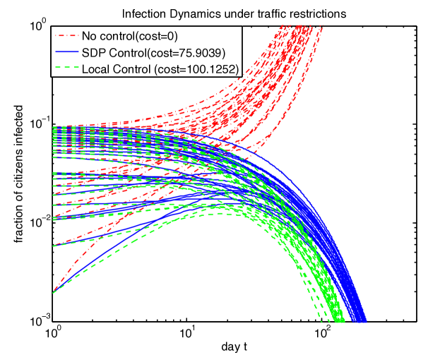
Figure VI.1: The fraction of people who are infected is driven to 0 in every city via traffic control. The cost incurred by the local heuristic is about 33% greater than the optimal cost.

We demonstrate the relative performance of our centralized and local solutions using a sample problem with randomly generated parameters. We choose the cost function

$$f(\omega)=-\sum_{(i,j)\in E}\ln\left(\frac{\omega_{ij}}{W_{ij}}\right)$$ (VI.1)

because it is convex and satisfies (V.1). Furthermore, (VI.1) intuitively captures the cost of restricting traffic on each edge because there is no cost when traffic is unrestricted (i.e. $w_{ij}=W_{ij}$) but the cost tends to $\infty$ as $w_{ij}\to 0$. It is not possible to completely delete an intercity connection.

Figure VI.1 shows that with no traffic restrictions all cities go to 100% infection rate while both the optimal solution and local heuristic force the virus to die out. The heuristic solution incurs a higher total cost but also forces the epidemic to die out faster.

Figure VI.2 shows the network of cities and the traffic restrictions on the edges. Points representing cities are scaled proportional to their populations $n_{i}$. Edges are scaled proportional to the the unrestricted traffic $W_{ij}$. The color of each edge is linearly scaled from green ($\omega_{ij}=W_{ij}$) to red ($\omega_{ij}=0$). It significant to note that despite the local approach, the restrictions imposed are very similar to the optimal case.

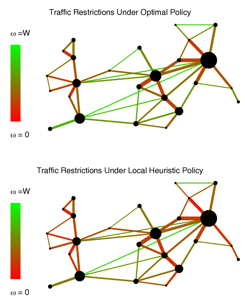
Figure VI.2: More traffic restrictions are required by the heuristic solution, however there is a strong correlation between which edges are restricted by the heuristic solution and by the optimal solution.

VII Conclusions

We have proposed a convex framework to contain the propagation of an epidemic outbreak in a metapopulation model by controlling the traffic between subpopulations. In this context, controlling the spread of an epidemic outbreak can be written as a spectral condition involving the eigenvalues of a matrix that depends on the network structure and the parameters of the model. Based on our spectral condition, we can find cost-optimal approaches to traffic control in epidemic outbreaks by solving an efficient semidefinite program.

References

- [1] R.M. Anderson and R.M. May, Infectious Diseases of Humans: Dynamics and Control, Oxford University Press, 1991.[27] I. Hanski and M. Gilpin, Metepopulation Biology: Ecology, Genetics and Evolution (Academic Press, San Diego, 1997).
- [2] P. Van Mieghem, J. Omic, and R. Kooij, “Virus Spread in Networks,” IEEE/ACM Transactions on Networking, vol. 17, no. 1, pp. 1–14, 2009.
- [3] I. Hanski and M. Gilpin, Metapopulation Biology: Ecology, Genetics and Evolution, Academic Press, 1997.
- [4] V. Colizza and A. Vespignani, “Epidemic Modeling in Metapopulation Systems with Heterogeneous Coupling Pattern: Theory and Simulations,” J. Theor. Biol., vol. 251, pp. 450-467, 2008.
- [5] P. Holland, K.B. Laskey, and S. Leinhardt, “Stochastic Blockmodels: Some First Steps,” Social Networks, vol. 5, pp. 109–137, 1983.
- [6] N. Biggs, Algebraic Graph Theory, Cambridge University Press, 1994.
- [7] K. Rohe, S. Chatterjee, and B. Yu, “Spectral clustering and the high-dimensional stochastic blockmodel,” The Annals of Statistics 39.4 (2011): 1878-1915.
- [8] R. Horn and C. R. Johnson. Matrix Analysis. Cambridge University Press, New York, 1985.