Frequency of Close Companions among Kepler Planets – a TTV study

Abstract

A transiting planet exhibits sinusoidal transit-time-variations (TTVs) if perturbed by a companion near a mean-motion-resonance (MMR). We search for sinusoidal TTVs in more than 2600 Kepler candidates, using the publicly available Kepler light-curves (Q0-Q12). We find that the TTV fractions rise strikingly with the transit multiplicity. Systems where four or more planets transit enjoy four roughly five times higher TTV fraction than those where a single planet transits, and about twice higher than those for doubles and triples. In contrast, models in which all transiting planets arise from similar dynamical configurations predict comparable TTV fractions among these different systems. One simple explanation for our results is that there are at least two different classes of Kepler systems, one closely packed and one more sparsely populated.

1. Introduction

Since the launch in March 2009, the Kepler mission has discovered a few thousand planetary candidates, called Kepler Objects of Interests (KOIs), by detecting the flux deficit as a planet transits in front of its star (Borucki et al., 2011; Batalha et al., 2013; Ofir & Dreizler, 2013; Huang et al., 2013; Burke et al., 2013). While some of the stars are observed to have one transiting planet (called “tranet” from now on, following Tremaine & Dong, 2012), others show up to 6 (Lissauer et al., 2011a). A natural question to ask is, do all of these systems share the same intrinsic orbital structures? For observing transiting planets, the two most relevant orbital parameters are the dispersion in orbital inclinations, and the typical spacing between adjacent planets.

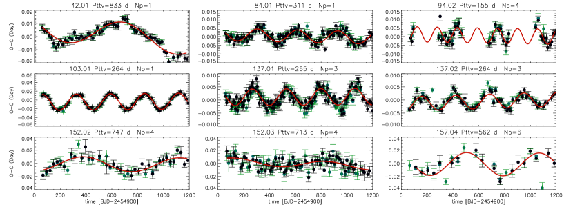
Figure 1.— A subset of TTV candidates identified with our standard criterion in the reduced KOI sample (case 1). The title of each panel indicates the KOI number, TTV super-period in days, and number of tranets in that system. In each panel we plot our measured TTV data points (black data) on top of the TTV measurements from Mazeh et al. (2013) (green data if any) as well as the best sinusoidal fit (red line). For data on all of our TTV candidates, see http://www.astro.utoronto.ca/$\sim$jwxie/TTV.

A number of groups have studied the inclination dispersion of Kepler planets and reached the common conclusion that this must be small and is of order a few degrees (Lissauer et al., 2011b; Fang & Margot, 2012; Tremaine & Dong, 2012; Fabrycky et al., 2012a; Figueira et al., 2012; Johansen et al., 2012). However, it has been pointed out that models with a single inclination dispersion falls short in explaining the number of single tranets relative to higher multiples, by a factor of three or more (Lissauer et al., 2011b). This suggests that all Kepler planets are not the same, and motivates models where the inclination dispersion itself is broadly distributed (“Rayleigh of Rayleigh”, Lissauer et al., 2011b; Fabrycky et al., 2012a). However, the relative occurrences of different Kepler multiples (denoted here as 1P, 2P, 3P… by the number of tranets seen in a system) are sensitive to both the inclination dispersion and the intrinsic planet spacing. Larger spacing between adjacent planets will raise the relative number of single tranet systems, as so will larger inclination dispersion. It is difficult to disentangle the two without the aid of further information. Therefore we turn to a new measure, the TTV fraction.

If a tranet is accompanied by another planet, its transit times deviate from strict periodicity (transit-time-variation, TTV, Holman & Murray, 2005; Agol et al., 2005). Many studies have used TTV to confirm the planetary nature of Kepler candidates (e.g. Holman et al., 2010; Lissauer et al., 2011a; Cochran et al., 2011; Ballard et al., 2011; Ford et al., 2012a; Steffen et al., 2012; Fabrycky et al., 2012b; Carter et al., 2012; Nesvorný et al., 2012; Xie, 2013a, b; Steffen et al., 2013). Furthermore, it is realized that when the companion is near a mean-motion resonance (MMR) with the tranet, the TTV is particularly strong and exhibits a characteristic sinusoidal form (Agol et al., 2005). The amplitude and phase of this sinusoid have been simply related to the perturber’s mass, as well as the orbital eccentricities (Lithwick et al., 2012), thereby allowing us to infer the interior composition and orbital parameters of these objects (Wu & Lithwick, 2013; Hadden & Lithwick, 2013).

Just as the TTV signal can be used to infer the presence of unseen (non-transiting) companions around specific candidates (e.g. Nesvorný et al., 2012; Nesvorný et al., 2013), the number of tranets that exhibit sinusoidal TTVs provides constraints on near-MMR companions. Since the period ratios of adjacent Kepler pairs do not much prefer MMRs (Fabrycky et al., 2012a), these near-MMR companions can be taken as a proxy for companions that lie close to and inward of the 2:1 MMR.

To be quantitative, we shall define the “intrinsic TTV fraction” as half the probability that a planet induces a sufficiently large TTV amplitude for detection in another planet in the system. The reason for the factor of a half is that when one planet has a large TTV, then typically so does its TTV partner, and we do not wish to double-count such a pair. When trying to measure this quantity observationally, we shall first count the number of observed tranets with measured TTV’s, and then subtract one each time two tranets are TTV partners. Dividing by the total number of tranets yields the “measured TTV fraction,” which is our estimate for the intrinsic fraction.

Our ability to measure TTV is affected by the noise level in the transit signals, which is in turn determined by a range of parameters including stellar brightness, the size of the planet relative to its host star, the orbital period and the transit duration. However, if we split the planet candidates into different groups, and if these groups share the same noise properties, then one can argue that the relative TTV fractions measured for different groups represent the relative differences in their intrinsic TTV fractions.

In the following, we proceed to measure the relative TTV fractions among 1P, 2P, 3P and 4P+ systems, where 4P+ stands for systems that have four or more transiting planets. We carry out the analysis for all KOIs that have suitable light-curves, which include more than 2600 KOIs. We interpret the significance of our results in §3.

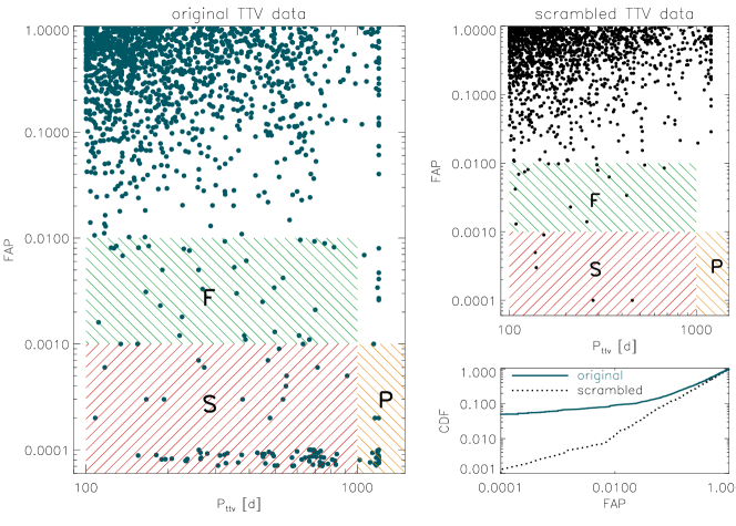
Figure 2.— The TTV periods and FAPs obtained for the full sample of 2606 KOIs. The left panel is for the original TTV data, while the right top panel pertains to a ‘scrambled’ population, one which has the same TTV data as the observed ones but with randomly scrambled time stamps. This set is equivalent to pure noise and acts as a control sample. For the sake of clarity, all points with FAP$<10^{-4}$ are displayed just below that value, with a slight artificial dispersion. The red hatched region labelled as ‘S’ illustrates our conservative criterion for identifying TTV candidates (§2.2), while more relaxed criteria include regions ‘F’ or ‘P’. The right-bottom panel shows the cumulative distribution of FAPs for the original TTV data (solid) and for the scrambled data (dashed). The latter satisfies CDF = FAP, as should be the case for pure noise. The real data show an excess of small FAP objects, over that of noise, corresponding to genuine TTV candidates. Small FAP cases, for the scrambled data, occur preferentially at short TTV periods.

2. Measuring TTV Fractions

2.1. Transit time measurements

We use the publicly available Q0-Q12 long cadence (LC, PDC) data for 2740 KOIs (Kepler objects of interest, Burke et al., 2013). Out of these, 134 KOIs have fewer than 7 transit time measurements, either because the transit periods are very long, or the signal-to-noise ratios (SNR) are too small. These spread evenly across all multiplicities. This leaves us with 2606 KOIs, out of which there are, 1488, 571, 320, 227 systems that are designated as 1P, 2P, 3P and 4P+, respectively. We refer to this sample of 2606 KOIs as the ‘full’ sample.

We have also selected a ‘reduced’ sample by excluding those KOIs for which timing measurements are less accurate. These include those with large noise ($SNR\leq 15$), and short transit duration (less than an hour). We include only KOIs with intermediate planet sizes ($0.8R_{\oplus}\leq R_{p}\leq 8R_{\oplus}$) as they likely have the lowest false positive rate (Fressin et al., 2013). This reduced sample contains a total of 1989 KOIs, with 1097, 446, 253, and 193 systems designated as 1P, 2P, 3P, and 4P+, respectively.

The pipeline used to measure the transit times has been developed and described in Xie (2013a). We compare our transit time measurements to the published ones (Ford et al., 2012a, b; Steffen et al., 2012; Fabrycky et al., 2012a; Mazeh et al., 2013), and found good consistency (see, e.g., Fig.1). Our measurements for the TTV candidates are publicly available at http://www.astro.utoronto.ca/$\sim$jwxie/TTV.

2.2. Identification of sinusoidal TTV

From the above transit time measurements, we derive TTV, which are the residuals after a best linear fit. We then search for a sinusoidal signal by obtaining a Lomb-Scargle (LS) periodogram (Scargle, 1982; Zechmeister & Kürster, 2009) on these residuals and identify the highest peak that has a period longer than twice the orbital period, as well as $>100$ days. The former threshold comes about because twice the orbital period is the Nyquist frequency for sampling TTV. The latter threshold is enforced because TTV at shorter periods can be significantly polluted by noise from chromospheric activities, as stellar rotation periods fall typically in the range from a few to a few tens of days (Szabó et al., 2013; Mazeh et al., 2013).

Sinusoidal TTV caused by a perturber near a MMR has a “super-period” (Agol et al., 2005; Lithwick et al., 2012),

$$P_{\rm ttv}\equiv{1\over{|j/P^{\prime}-(j-1)/P|}}={{P^{\prime}}\over{j|\Delta|}},$$ (1)

where $P$ and $P^{\prime}$ are the orbital periods of the two planets that are near a first-order $(j:j-1)$ MMR by a fractional distance $\Delta$. For a planet pair with period $P^{\prime}=10$ days, $j=2$, $|\Delta|\sim 5\%$, we find $P_{\rm ttv}\sim 100$ days. A planet pair with a larger $|\Delta|$ will have a shorter super-period, however their TTVs also become increasingly difficult to detect as the TTV amplitudes scale inversely with $|\Delta|$ (Agol et al., 2005; Lithwick et al., 2012). All reported cases (Lithwick et al., 2012; Xie, 2013a, b; Wu & Lithwick, 2013; Steffen et al., 2012; Ragozzine & Kepler Team, 2012) have $|\Delta|$ falling between $1-5\%$. This consideration, coupled with the above concern for chromospheric noise, leads us to discard sinusoids short-ward of 100 days.

We also adopt an upper limit of $P_{\rm ttv}\leq 1000$ days. This comes about because the data (Q0-Q12) stretch only $\sim 1100$ days. However, some TTV systems show strong, identifiable sinusoids even before a full TTV cycle is observed. This constraint is later relaxed and is found not to impact the conclusion.

Many of the sinusoids thus identified are false, caused by random alignment of noisy data. It is an important task to exclude these. We adopt the following strategy from Cumming (2004), originally applied to detect planets from radial velocity data. For each KOI, we scramble the time stamps of the original TTV data for $10^{4}$ times, perform a LS periodogram analysis on each set of data, obtaining the amplitude and frequency on the highest peak. The FAP (false alarm probability) of the original TTV peak is estimated as the fraction of permutations that have higher sinusoids than the original TTV. We assign an FAP value of $10^{-4}$ if not a single random realization exceeds the observed sinusoid amplitude. Our FAP estimates compare well with those from Mazeh et al. (2013).

Fig.2 shows the FAP and $P_{\rm ttv}$ for each of the KOIs in our full sample, as well as those using a scrambled time series for the same KOIs. The latter set is equivalent to random noise and so acts as a control sample. The true data show a significant excess of objects at very low FAPs, when compared to those of the scrambled data. We adopt the following ‘standard’ criterion (the region labelled as ‘S’ in Fig. 2) for identifying our TTV candidates:

• (1) $\rm FAP<10^{-3}$ and

• (2) TTV period between 100 and 1000 d.

Objects that have FAP $\leq 10^{-3}$ exhibit TTV amplitudes that range from one to hundreds of minutes, with TTV sensitivity higher for larger SNR objects. Our above FAP criterion is on the conservative side: for an FAP of $10^{-3}$, there should only be $2606\times 10^{-3}\sim 3$ false positives among our TTV candidates, much fewer than the actual number of candidates ($\sim 100$). We experiment by relaxing the above criterion, either by raising the FAP threshold to $10^{-2}$ (adding the ‘F’ region in Fig. 2), or by removing the 1000 day upper limit (adding the ‘P’ region). We report our results below.

Table 1TTV fraction as a function of transit multiplicity

case	KOIsa	TTVsa	1P		2P		3P		4P+
			$N_{\rm ttv}/N_{\rm koi}$b	$\%$c	$N_{\rm ttv}/N_{\rm koi}$	$\%$	$N_{\rm ttv}/N_{\rm koi}$	$\%$	$N_{\rm ttv}/N_{\rm koi}$	$\%$
0	full	S	(31)31/1488	2.1$\pm$0.4	(24)19/571	3.3$\pm$0.8	(19)13/320	4.1$\pm$1.1	(23)17/227	7.5$\pm$1.8
1	reduced	S	(19)19/1097	1.7$\pm$0.4	(24)19/446	4.3$\pm$1.0	(16)13/253	5.1$\pm$1.4	(23)17/193	8.8$\pm$2.1
2	reduced	S + P	(26)26/1097	2.4$\pm$0.5	(32)26/446	5.8$\pm$1.1	(22)16/253	6.3$\pm$1.6	(28)21/193	10.9$\pm$2.4
3	reduced	S + F	(38)38/1097	3.5$\pm$0.6	(37)31/446	7.0$\pm$1.2	(25)20/253	8.0$\pm$1.8	(28)20/193	10.4$\pm$2.3

^a See §2 for definitions of various samples and TTV thresholds. The ‘reduced’ sample is selected based on SNR, transit duration, and luminosity; the S, P, and F criteria are illustrated in Fig. 2.
^b Number of identified TTV candidates, versus numbers of KOIs in that category. The numbers in parentheses are the raw TTV candidates, while the the corrected ones after parentheses result from removing one of the two TTV candidates from the count whenever a TTV pair is seen.
^c The measured TTV fraction using the corrected TTV count.

2.3. TTV Fraction & Multiplicity

We observe a remarkable rise of the TTV fraction with transit multiplicity.

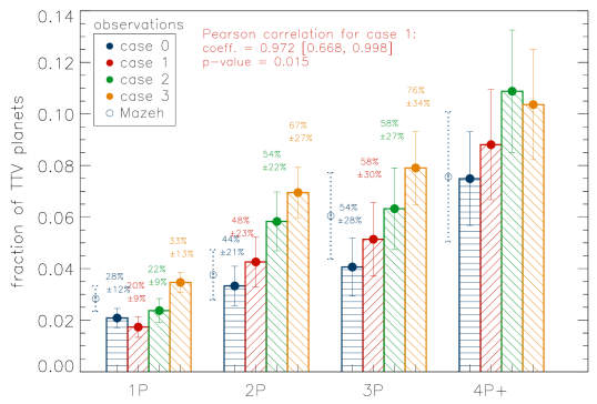
Figure 3.— The measured TTV fraction in 1P, 2P, 3P and 4P+ systems, for the 4 combination of selection thresholds described in Table 1. The error bars are $1-\sigma$ Poisson error in each case. Within each transit group, the TTV fractions rise as we relax the criterion for identifying TTV candidates (from case 1 to 2 to 3). The TTV fractions for case 0 (full sample) are somewhat lower than for case 1 (reduced sample), as we are more sensitive to the presence of TTV in the reduced sample. The percentages printed above each column stand for the relative TTV fraction, normalized by that in the 4P+ group. The occurrence rate of sinusoidal TTV is much lower in singles than those in higher multiples. Results obtained using the TTV catalogue of Mazeh et al. (2013) , with selection criteria equivalent to our case 0, are shown as open circles and are consistent with our values. The Pearson statistics (Rodger & Nicewander, 1988) shows that the TTV fraction is positively correlated with the transit multiplicity (correlation $r=0.97$ with $1$ being perfect linear correlation), and that the correlation is statistically significant – the null-hypothesis (no correlation) is strongly rejected with a p-value of $0.015$. From Monte-Carlo simulations , we obtain a $95\%$ confidence interval for the correlation coefficient from 0.668 to 0.998 given the error bars of TTV fractions in case 1.

In Table 1, we list the number of TTV candidates for different transiting multiplicities, for four different combinations of sample and TTV selection criteria. For ease of comparison against theory, we list the “measured” TTV fractions, obtained by removing one candidate from the raw count whenever both it and its TTV partner have observed TTVs. Such a method is justified in §3. From now on, we focus on these “measured” fractions (illustrated in Fig. 3) – in fact, we focus on the relative “measured” fractions, the TTV fractions normalized by that in 4P+ systems. The choice for the normalization is arbitrary. However, since the errorbars for these relative fractions are taken to be quadratic sums of the individual errorbars, which type of system one normalizes against does not affect the statistical conclusion. These results are presented in Fig. 3.

Except for case 3, all other combinations give very similar results for the relative TTV fractions: 1P systems have about five times lower (values from case 1: $20\pm 9\%$) TTV fraction than 4P+, and 2P and 3P systems are about twice lower ($48\pm 23\%$, and $58\pm 30\%$). Results from case 3 are less reliable as the TTV selection criterion is too relaxed and allows for too many false positives.

We have also used the TTV data from Mazeh et al. (2013), published while we are editing our final draft, to confirm the above results (Fig. 3).

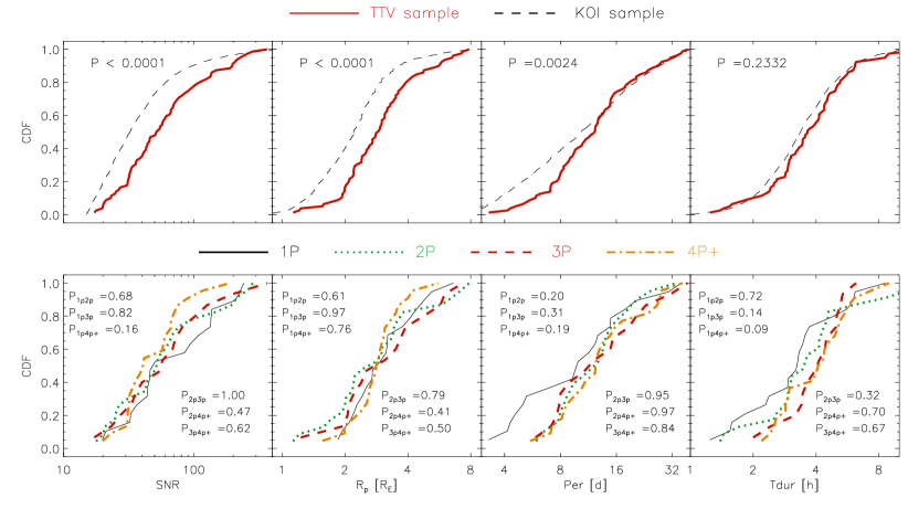
Figure 4.— Comparison of properties. The top panels compare those with sinusoidal TTV (red solid curve) to all KOIs (black dashed curve). The lower panels compare TTV candidates with different transit multiplicities. Here we only display comparison in transit signal-to-noise ratio (SNR), planet radius ($\rm R_{p}$), orbital period (Per) and transit duration, but we have performed a range of other ones (see text). TTV detection disfavours planets with small SNR and small radius ($R_{p}\leq 2R_{E}$), and favours planets with intermediate orbital periods ($P\sim 10$ day). In contrast, TTV groups with different multiplicities are statistically indistinguishable in these transit parameters (p-values from KS tests are listed).

2.4. Potential Bias

We first discuss what potential bias may affect the absolute TTV fractions that we obtain, then move on to discuss biases that may affect the relative TTV fractions among groups of different transit multiplicity. It becomes clear that by focusing only on the relative TTV fractions, we can eliminate many , if not all, observational bias.

We compare properties of the set of TTV candidates against the KOI sample. The top panels of Fig. 4 display four transit properties: signal-to-noise ratio, planet radius, orbital period and transit duration. The TTV sample have in general larger transit SNR, larger planet radii (disfavouring small planets) and slightly longer transit durations than the average KOIs. In addition, they are also concentrated around orbital periods $\sim 10$ days. These characteristics allow for optimum TTV detections , as is demonstrated in recent TTV studies by Ford et al. (2012b); Mazeh et al. (2013). For instance, longer orbital periods generally lead to larger TTV amplitudes (Holman & Murray, 2005; Agol et al., 2005; Lithwick et al., 2012; Mazeh et al., 2013), yet too long orbital periods permit only a small number of transits to be observed. As such, we expect that the intrinsic TTV fraction, quantified as half the fraction of planets that have comparable TTV amplitudes as the ones detected here, should be higher than our reported values (Table 1).

On the other hand, we find no significant difference between the TTV and KOI samples in terms of stellar mass, effective temperature, metallicity and stellar brightness (stellar parameters from Batalha et al., 2013). KS tests performed to compare these two populations always return p-values greater than $0.5$. This suggests that TTV candidates live in all possible systems. However, this deserves further study as currently there are large uncertainties in stellar parameters, and our TTV sample is relatively small.

While the TTV sample as a whole are a biased representation of the KOI sample, we find that the different sub-samples, separated by their transiting multiplicity, share similar distributions in both the transit parameters (Fig.4) and the stellar parameters (not shown here). The large p-values returned from KS tests (Fig.4) do not support the hypothesis that the different subgroups experience different selection effects. Moreover, we have confirmed that our reduced KOI samples, when separated into groups of different transit multiplicities, are statistically similar in their transit and stellar parameters. Since the ability to detect TTV above a certain threshold amplitude, only depends on these transit and stellar parameters, these two results then argue that the relative measured TTV fractions reflect the relative intrinsic TTV fractions. In other words, the significant correlation between TTV fraction and transit multiplicity that we observe (Fig.3) is unlikely to be caused by systematic biases on stellar/transit parameters.

Another potential bias could arise during transit detection – transiting planets with significant TTVs can be systematically missed, or cataloged as false positives by the Kepler pipeline García-Melendo & López-Morales (2011). To remove this bias, Carter & Agol (2013) designed an algorithm (QATS) that can simultaneously detect transits and measure their TTVs. Searches using QATS have only found a handful of new planetary candidates (private communication J. A. Carter), which might indicate that the Kepler catalogue is not significant impacted by this bias. Nevertheless, we caution that there could be another possibility, namely, the QATS could not fully remove the bias, which deserves further study but is out of the scope of this paper.

Last but not least, we note that the transit multiplicity of a given system is evolving as the catalog updates. For example, a 1P system may become a 2P system when a new transit candidate is found , either due to accumulation of new data and/or improvement of the pipeline/algorithm for planet detection. To see how these factors affect our results, we took an older version KOI catalog from Batalha et al. (2013) and performed the same analysis as done in the standard case (case 1 in table 1). We obtained similar results for the relative TTV fractions: ($2.4\pm 0.5)\%$, ($4.9\pm 1.1)\%$, ($6.0\pm 1.7)\%$ and ($10.3\pm 3.0)\%$ for the 1P, 2P, 3P and 4P systems, respectively. This suggests that the correlation between TTV fraction and transit multiplicity observed in Fig. 3 may remain unaffected as more improved catalogues are published.

3. Conclusion

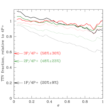
Figure 5.— Theoretical TTV fractions for different multiplicity groups, measured relative to that in 4P+ systems. Here, we construct a ensemble of planetary systems where the period ratio between neighbouring planets $x=P_{2}/P_{1}$, satisfies a Rayleigh distribution $P(x)=x/\sigma^{2}\,e^{-x^{2}/2\sigma^{2}}$, and where the planets’ mutual inclinations are described by an independent Rayleigh distribution with $\sigma_{\rm inc}=3\deg$. The results presented here are insensitive to the value of $\sigma_{\rm inc}$. We identify TTV planets as those that transit their host stars and have a companion within a fractional distance of $2\%$ from a first-order MMR. The solid lines indicate the measured fractions, while the dotted lines are the raw fractions (i.e., the fraction before removing doubly-counted TTV pairs), plotted as functions of $\sigma$, for different multiplicity groups. The raw fractions in the 1P systems can drop to half of that in the 4P systems, because one is likely to observe both planets in the same TTV pair in the latter case. In contrast, in the corrected form (our so-called ’measured’ TTV fraction), the relative TTV fractions remain close to unity, and are largely independent of either transit multiplicity or model parameters. In contrast, the observed relative fractions (case 1 in Fig. 3, marked here as arrows) fall much below unity.

We discuss the significance of our results by contrasting them against predictions from a simple toy model. Assume all KOIs, independent of transit multiplicity, are drawn from the same intrinsic distribution, with similar dispersions in mutual inclinations and planet spacing (with no preference for MMRs). In this case, single systems are the ones where the viewing angles are less favourable and we miss most of the planets in the system, while the higher multiples are ones where more planets are caught. One can estimate the TTV fraction for the theoretical population as half the fraction of planets that both transit and have companions within a certain distance from a first-order MMR. As one naively expects and as is confirmed by Monte Carlo simulations (Fig. 5), the relative TTV fractions cluster around $1$, and are largely independent of the model parameters and transit multiplicities.

The observed sharp rise of TTV fraction with transit multiplicity is inconsistent with such a simple toy-model. What are the possible interpretations?

The lower TTV fraction observed for singles is unlikely to be completely explained by the higher false positive rates in KOI singles. The reported false positive rate is of order $10-20\%$ (Fressin et al., 2013). More importantly, our reduced sample, which is expected to have a lower false positive rate than the full sample, yields the same relative TTV fractions. Moreover, since TTV amplitudes are strongly boosted by eccentricities as small as a few percent (Holman & Murray, 2005; Agol et al., 2005; Veras et al., 2011; Lithwick et al., 2012), the lower TTV fraction can be explained if higher multiple systems have higher eccentricities. However, this is likely excluded by the tight spacing observed among high multiples.

A simple explanation for our results is that the basic assumption in our toy model is not true, namely, all KOIs cannot be treated as the same intrinsic population (Lissauer et al., 2011b; Tremaine & Dong, 2012; Johansen et al., 2012; Weissbein et al., 2012). For example, there could be at least two distinct populations of Kepler planets, different in their intrinsic frequencies of close companions. The high multiples (4P+) are dominated by a population that has a higher companion frequency, while the 1P systems may be dominated by a population that have a lower frequency of close companions. In other words, there are at least two populations of Kepler planets, one that are closely spaced, and one that is sparsely spaced. In an upcoming publication, we will use TTV fractions obtained in this paper, together with a variety of other observational facts, to constrain the properties of these two populations of Kepler planets. This will yield important constraints on the process of planet formation.

References

- Agol et al. (2005) Agol, E., Steffen, J., Sari, R., & Clarkson, W. 2005, MNRAS, 359, 567
- Ballard et al. (2011) Ballard, S., et al. 2011, ApJ, 743, 200
- Batalha et al. (2013) Batalha, N. M., et al. 2013, ApJS, 204, 24
- Borucki et al. (2011) Borucki, W. J., et al. 2011, ApJ, 736, 19
- Burke et al. (2013) Burke, C. J., Bryson, S., Christiansen, J., Mullally, F., Rowe, J., Science Office, K., & Kepler Science Team. 2013, in American Astronomical Society Meeting Abstracts, Vol. 221, American Astronomical Society Meeting Abstracts, 216.02
- Carter et al. (2012) Carter, J. A., et al. 2012, Science, 337, 556
- Carter & Agol (2013) Carter, J. A., & Agol, E. 2013, ApJ, 765, 132
- Cochran et al. (2011) Cochran, W. D., et al. 2011, ApJS, 197, 7
- Cumming (2004) Cumming, A. 2004, MNRAS, 354, 1165
- Fabrycky et al. (2012a) Fabrycky, D. C., et al. 2012a, ArXiv e-prints
- Fabrycky et al. (2012b) —. 2012b, ApJ, 750, 114
- Fang & Margot (2012) Fang, J., & Margot, J.-L. 2012, ApJ, 761, 92
- Figueira et al. (2012) Figueira, P., Marmier, M., Boué, G., et al. 2012, A&A, 541, A139
- Ford et al. (2012a) Ford, E. B., et al. 2012a, ApJ, 750, 113
- Ford et al. (2012b) —. 2012b, ApJ, 756, 185
- Fressin et al. (2013) Fressin, F., et al. 2013, ApJ, 766, 81
- García-Melendo & López-Morales (2011) García-Melendo, E., & López-Morales, M. 2011, MNRAS, 417, L16
- Hadden & Lithwick (2013) Hadden, S., & Lithwick, Y. 2013, arXiv:1310.7942
- Holman & Murray (2005) Holman, M. J., & Murray, N. W. 2005, Science, 307, 1288
- Holman et al. (2010) Holman, M. J., et al. 2010, Science, 330, 51
- Huang et al. (2013) Huang, X., Bakos, G. Á., & Hartman, J. D. 2013, MNRAS, 429, 2001
- Johansen et al. (2012) Johansen, A., Davies, M. B., Church, R. P., & Holmelin, V. 2012, ApJ, 758, 39
- Lissauer et al. (2011a) Lissauer, J. J., et al. 2011a, Nature, 470, 53
- Lissauer et al. (2011b) —. 2011b, ApJS, 197, 8
- Lithwick et al. (2012) Lithwick, Y., Xie, J., & Wu, Y. 2012, ApJ, 761, 122
- Mazeh et al. (2013) Mazeh, T., Nachmani, G., Holczer, T., et al. 2013, ApJS, 208, 16
- Nesvorný et al. (2013) Nesvorný, D., Kipping, D., Terrell, D., et al. 2013, ApJ, 777, 3
- Nesvorný et al. (2012) Nesvorný, D., Kipping, D. M., Buchhave, L. A., Bakos, G. Á., Hartman, J., & Schmitt, A. R. 2012, Science, 336, 1133
- Ofir & Dreizler (2013) Ofir, A., & Dreizler, S. 2013, A&A, 555, A58
- Ragozzine & Kepler Team (2012) Ragozzine, D., & Kepler Team. 2012, in AAS/Division for Planetary Sciences Meeting Abstracts, Vol. 44, AAS/Division for Planetary Sciences Meeting Abstracts, 200.04
- Rodger & Nicewander (1988) Rodgers, J. L. and Nicewander W. A., 1988, The American Statistician Vol. 42, No. 1, pp. 59-66
- Scargle (1982) Scargle, J. D. 1982, ApJ, 263, 835
- Steffen et al. (2012) Steffen, J. H., et al. 2012, MNRAS, 421, 2342
- Steffen et al. (2013) —. 2013, MNRAS, 428, 1077
- Steffen (2013) Steffen, J. H. 2013, MNRAS, 433, 3246
- Szabó et al. (2013) Szabó, R., Szabó, G. M., Dálya, G., Simon, A. E., Hodosán, G., & Kiss, L. L. 2013, A&A, 553, A17
- Tremaine & Dong (2012) Tremaine, S., & Dong, S. 2012, AJ, 143, 94
- Veras et al. (2011) Veras, D., Ford, E. B., & Payne, M. J. 2011, ApJ, 727, 74
- Weissbein et al. (2012) Weissbein, A., Steinberg, E., & Sari, R. 2012, arXiv:1203.6072
- Wu & Lithwick (2013) Wu, Y., & Lithwick, Y. 2013, ApJ, 772, 74
- Xie (2013a) Xie, J.-W. 2013, ApJS, 208, 22
- Xie (2013b) Xie, J.-W. 2014, ApJS, 210, 25
- Zechmeister & Kürster (2009) Zechmeister, M., & Kürster, M. 2009, A&A, 496, 577