Laplacian-based generalized gradient approximations for the exchange energy

Abstract

It is well known that in the gradient expansion approximation to density functional theory (DFT) the gradient and Laplacian of the density make interchangeable contributions to the exchange correlation (XC) energy. This is an arbitrary “gauge” freedom for building DFT models, normally used to eliminate the Laplacian from the generalized gradient approximation (GGA) level of DFT development. We explore the implications of keeping the Laplacian at this level of DFT, to develop a model that fits the known behavior of the XC hole, which can only be described as a system average in conventional GGA. We generate a family of exchange models that obey the same constraints as conventional GGA’s, but which in addition have a finite-valued potential at the atomic nucleus unlike GGA’s. These are tested against exact densities and exchange potentials for small atoms, and for constraints chosen to reproduce the SOGGA and the APBE variants of the GGA. The model reliably reproduces exchange energies of closed shell atoms, once constraints such the local Lieb-Oxford bound, whose effects depend upon choice of energy-density gauge, are recast in invariant form.

I Introduction

I.1 The exchange-correlation energy and hole

The basic issue of density functional theory Hohenberg and Kohn (1964); Dreizler and Gross (1990); Jones and Gunnarsson (1989) (DFT) is modeling the exchange-correlation (XC) energy – the description of the electron-electron interaction energy due to Fermi statistics and many-body interactions within a single-particle formulation of the ground-state problem. Beyond the very basic local density approximation (LDA) which maps the XC energy-per-particle at any point in space to that of the homogeneous electron gas (HEG), Kohn and Sham (1965) there is no truly systematic approach to building functionals. A heuristic paradigm that provides some structure to the problem is that of a Jacob’s ladder Perdew and Schmidt (2001) of functionals, where these are grouped in families (rungs on the ladder) with each successive rung characterized by an increase in the amount of information about the system being used. Generally, this leads to functionals of increasing sophistication and accuracy as one moves up the ladder, but with the tradeoff of increasing complexity and computational cost.

Left unsaid is how one is to obtain the best description of nature within a given class or rung of functionals. A good example of this lack of systematizability within a class is the low-level generalized gradient approximation (GGA) family of functionals that employ the gradient of the density as well as the local value of the density to construct local XC energies. This class of functional is extremely popular, easy to implement and use, but not quite robust enough for enough applications to be a completely satisfactory workhorse for electronic structure calculations. There has thus been much effort to optimize the GGA and dozens of published functionals. Taking one commonly used functional, the PBE, PBE variants have been developed to optimize it either for specific applications such as atomization energies for molecules, Hammer, Hansen, and N$\o$rskov (1999); Zhang and Yang (1998); Constantin et al. (2011); del Campo et al. (2012) structural constants, particularly of solids, Wu and Cohen (2006); Zhao and Truhlar (2008) or solid surface energies, Perdew et al. (2008) or for broad applicability. Ruzsinszky, Csonka, and Scuseria (2009); Fabiano, Constantin, and Della Sala (2010); Haas et al. (2010) It has been argued that a GGA in principle does not include enough information to reach all these goals. Perdew et al. (2006, 2009)

A particularly fruitful approach to understanding the XC energy has been the XC hole, $n_{xc}({\bf r},{\bf r}^{\prime})$, defined as the change in electron density from the mean at ${\bf r}^{\prime}$ given the presence of an electron observed to be at ${\bf r}$. An exchange-correlation energy-per-particle $\epsilon_{XC}$ at any point ${\bf r}$ can then be defined as the net change in energy due to the formation of the hole about an electron placed at ${\bf r}$. This includes the potential energy gain due to the interaction of the electron with its own hole and the kinetic energy cost to create it. The net effect is obtained through an adiabatic formulationHarris and Jones (1974); Langreth and Perdew (1975); Gunnarson and Lundqvist (1976)

$$\epsilon_{XC}({\bf r})=\frac{1}{2}\int d\lambda\;\int_{0}^{1}d^{3}r^{\prime}\;\frac{n_{XC}^{\lambda}({\bf r},{\bf r}^{\prime})}{\left|{\bf r}-{\bf r}^{\prime}\right|}.$$ (1)

(Throughout this paper, expressions are written in hartree atomic units.) Here $n_{XC}^{\lambda}$ is the XC hole evaluated for a system with Coulomb coupling $\lambda e^{2}$ and the same ground-state density $n({\bf r})$ as the true system. The coupling constant varies from noninteracting (0) to fully interacting (1) systems. The total XC energy is obtained from $\epsilon_{XC}$ by integration over ${\bf r}$:

$$E_{xc}=\int d^{3}r\;e_{XC}({\bf r})=\int d^{3}r\;n({\bf r})\epsilon_{XC}({\bf r}).$$ (2)

where $e_{XC}({\bf r})=n({\bf r})\epsilon_{XC}({\bf r})$ is the local XC energy density. The LDA can then be derived by parametrizing $\epsilon_{XC}({\bf r})$ in terms of the local density $n({\bf r})$ and the GGA by both local density and gradient $\nabla n({\bf r})$.

The close connection between the XC hole and energy historically provided a theoretical basis to explain the surprising successJones and Gunnarsson (1989) of the LDA and to to construct widely-used DFT’s including the PBE,Perdew, Burke, and Wang (1996) and hybrids with Hartree-Fock.Becke (1993) The XC hole has played a supporting role in recent developments in modeling the XC potential, Becke and Johnson (2006); Becke and Roussel (1989) as well as sophisticated “Koopman’s compliant” functionals to treat many-electron self-interaction error; Dabo et al. (2010) the adiabatic connection also continues to be of importance in a variety of contexts. Cohen, Mori-Sánchez, and Yang (2012)

I.2 Revisiting the gradient expansion

A major problem with using the energy density $e_{XC}$ to define a XC functional is that it is not uniquely defined. Adding any functional of the density that integrates to zero for any density will define a new $e_{XC}$ while leaving the XC energy, and thus the physics of the system, unchanged. This is not hard to do – for example, the addition of a divergence of a vector functional is enough:

$$e_{XC}^{\prime}=e_{XC}[n]({\bf r})+\nabla\cdot{\bf v}[n]({\bf r}),$$ (3)

as long as the related flux integral can be set to zero on the boundary. If such a relation between $e_{XC}$ and $e_{XC}^{\prime}$ holds for every possible density $n({\bf r})$, then the total energy and also the potential $\delta E_{XC}/\delta n({\bf r})$ of each will be indistinguishable from each other. This ambiguity is thus similar to that of the gauge of the potential in classical electrodynamics.

The gauge ambiguity in defining $e_{XC}$ played a role from the very beginning of DFT with the gradient expansion. Hohenberg and Kohn (1964) Hohenberg and Kohn, in their seminal paper on DFT note that the gradient expansion for a system with a slowly varying density should most generally be expressed as

$$e^{GEA}_{XC}[n]=e_{XC}^{0}[n]+\left\{e_{XC}^{(2a)}[n]\nabla^{2}n+e_{XC}^{(2b)}[n]|\nabla n|^{2}\right\}+O(\nabla^{4})$$ (4)

with two second order terms, involving the gradient and the Laplacian of the density. With the addition of the pure divergence $\nabla\cdot(-e_{XC}^{(2a)}\nabla n)$, the energy density can be converted into a form exclusively involving the gradient-squared of the density, obviating the need of a Laplacian term entirely and making life simpler for modelers.

Nevertheless, there are reasons for exploring the gauge freedom to construct DFT from different starting points. It has been a long standing issue of DFT’s that build upon the gradient-only form of the GEA that the XC potentials they produce have a false $1/r$ singularity in the XC potential in the vicinity of the atomic nucleus, induced by the cusp in the charge density in this limit. However, it is easy Umrigar and Gonze (1994) to construct a finite potential if one has access to the Laplacian.

Secondly, by transforming $\epsilon_{XC}$ to a gradient-only form, the fruitful connection between XC energy and XC hole becomes obscured. We show below that the local energy of the X hole in the gradient expansion limit is necessarily a functional of both the gradient and the Laplacian; although an accurate local energy is not needed to get correct total exchange energy, it helps to have a correct local energy to analyze trouble areas like the 1s shell and nuclear cusp. Moreover, by eliminating the Laplacian of the density, one is discarding information about the topology of an electronic system that is potentially useful, especially if tied back to the XC hole. For example, the Laplacian is known to be a faithful indicator of shell structure and useful in diagnosing the ionicity of bonds, used for this purpose in the Atoms in Molecules approach to visualizing molecular structure and reactions. (Bader and Essen, 1983; Bader et al., 1996)

This issue has been highlighted by recent work modeling data for the exchange-correlation hole from variational quantum Monte Carlo (VMC) studies. Cancio and Chou (2006) Recent simulations have obtained data for the adiabatically integrated XC hole and energy density using highly accurate VMC methods for calculating the expectations of an optimized many-body wavefunction and explicit coupling-constant integration.Hood et al. (1998) These include the Si crystal,Hood et al. (1997, 1998); Cancio, Chou, and Hood (2001) atoms,Cancio, Fong, and Nelson (2000); Puzder, Chou, and Hood (2001); Cancio and Fong (2012) and small organic moleculesHsing, Chou, and Lee (2006) within a pseudopotential approximation, and a model charge-density-wave system.Nekovee, Foulkes, and Needs (2001, 2003) The outstanding feature of all these studies is the strong correlation between the local Laplacian of the density and the error in the LDA model for the adiabatically integrated XC energy density, measured with respect to the VMC data. The correlation is unmistakable and cannot be described in terms of alternate variables such as the kinetic energy density or the gradient of the density. An empirical fit of this difference for the Si crystal to a Laplacian-based enhancement factor of the LDA energy, constructed in analogy to a GGA, recovers 70% of the energy difference between the VMC and the LDA for most of the systems studied.Cancio and Chou (2006)

Thus VMC data indicate that possibly we should rethink the GGA “rung” in the Jacob’s ladder for DFT. Apparently nature, or at least the adiabatic XC hole is better described using a different “gauge” choice than that of the classic GGA, and designing a GGA based on such a gauge may help us to use the insights from XC hole calculations more effectively. And the extra degree of freedom allows for applying constraints that are not possible in the classic GGA, such as the character of the XC potential at the nucleus. It is possible also that redefinition of the GGA in terms of the Laplacian might lead to better ground state predictions, such as that of covalently bonded systems such as the Si crystal.

The Laplacian of the density has not been used much in DFT, with but a few explicit models Perdew and Constantin (2007) in recent years. One approach to DFT that does employ them is complementary to one taken here – use of X and C holes to define corresponding potentials, with a fit to the expansion of the exact exchange hole to determine shape and extent of hole. Becke and Roussel (1989) Laplacian terms naturally arise there for the same reason as they do in this paper, from the description of the exchange hole, while the approach is computationally quite a bit more intensive than a GGA, and belongs on the higher “metaGGA” class of functionals. This approach has had a revival in recent years, Becke and Johnson (2006); Rasanen, Pittalis, and Proetto (2010); Tran and Blaha (2009) producing very accurate potentials and improved semiconductor band-gaps. However the path back to extracting useful XC energies from potentials is nontrivial. Gaiduk and Staroverov (2012)

Finally, we note the relevance of this work to the development of orbital-free DFT’s. Explicit functionals of the density, eliminating the step of constructing orbitals as must be done for the kinetic energy density in the Kohn-Sham approach, would be of great usefulness for extending the capability of DFT. This is especially true for application to warm dense matter where both the conditions of quantum mechanics and high temperature (thus high orbital occupancies) must be dealt with. Karasiev, D.Chakraborty, and Trickey (2013) Laplacian-based XC functionals are of interest in this context as potential candidates to replace meta-GGA’s which currently rely upon the Kohn-Sham kinetic energy density, and thus require the use of orbitals. And the techniques developed here for implementing this variable in the XC functional may be of use for KE functionals as well.

The focus of this paper is on designing a mature, robust functional for exchange. Correlation is, to a large degree, a response to exchange, and as a result, parameters and functional forms for correlation are chosen to fit with the given form for exchange. At the same time, correlation tends to be considerably more complex than exchange because it lacks the simple scaling behavior under uniform coordinate scaling that restricts exchange to a relatively simple form. Nevertheless many of the techniques discussed here should be applicable to correlation as well.

In a preliminary attempt at the design of a Laplacian-based GGA for exchange, Cancio, Wagner, and Wood (2012) we demonstrated the possibility of using the Laplacian in combination with the gradient of the density in density functional theory in an all-electron context, going beyond the pseudopotential approximations used in QMC. We focused on resolving technical issues of controlling nonlinear behavior in the exchange-correlation potential due to the use of Laplacian and poor choices for the form of the functional. In this paper, we develop and construct an effective set of “gauge invariant” constraints based on those of PBE, requiring us to revisit especially the bounds in the limit of large inhomogeneity. The use of the Laplacian allows (and requires) one to satisfy a number of constraints on the potential in addition to the energy, which results in a more robust functional. We test our functional against numerically exact densities and potentials for small atoms and against densities and energies derived from the APBE functional Constantin et al. (2011) for large atoms. The end result is an effective and mature exchange functional that reproduces GGA energies for atoms and fixes the problem of the GGA potential at the nucleus.

Section II discusses in detail the theory behind our functional, especially the constraints used; Section III is a short description of numerical techniques used in testing our functionals. Energies and potentials for example atoms are discussed in Section IV and Section V includes a discussion of possible future steps and our conclusions.

II Theory

We start with the basic form of the PBE functional, perhaps the most commonly used constraint-based GGA and the generator of a large family of derivative functionals. Ignoring spin polarization, the PBE energy density is given by:

$$\begin{split}e^{PBE}_{xc}(n,\nabla n)=F^{PBE}_{X}(s^{2})e_{X}^{LDA}(r_{s})\\ +\>e_{C}^{LDA}(r_{s})+H^{PBE}_{C}(r_{s},t^{2}).\end{split}$$ (5)

where the two basic order parameters characterizing the energy are the Wigner-Seitz radius $r_{s}\!=\!{3/4\pi n}^{1/3}$, and a scale-invariant inhomogeneity parameter,

$$s^{2}=\frac{|\nabla n|^{2}}{4k_{F}^{2}n^{2}},$$ (6)

with $k_{F}\!=\!(3\pi^{2}n)^{1/3}\!\sim\!1/r_{s}$ being the local Fermi wavevector. The LDA exchange energy density is $e_{x}^{LDA}\!=\!-3k_{F}n/4\pi$ and scales with density as $n^{4/3}$. It shows the correct behavior under an important scaling transformation – the uniform scaling of coordinates $r\!\rightarrow\!\gamma r$, $n(r)\!\rightarrow\!\gamma^{3}n(\gamma r)$. To preserve this behavior, the GGA correction is restricted in form to a multiplicative enhancement factor $F_{X}$ parameterized solely in terms of scale-invariant quantities such as $s^{2}$.

The LDA correlation energy density is a function of $r_{s}$ with non-trivial scaling behavior. The correlation correction $H_{C}$ is, likewise, a more complex functional than its exchange counterpart, depending on a inhomogeneity parameter $t^{2}$ that is defined with respect to the Thomas-Fermi screening vector $k_{s}\!=\!\sqrt{4k_{F}/\pi a_{0}}$. This does not introduce a new variable to the functional, as it reduces to a function of $s^{2}$ and $k_{F}$:

$$t^{2}=(k_{F}/4\pi)s^{2}$$ (7)

The additive form of the generalized gradient correction for correlation, $H_{C}$, is, like the multiplicative form $F_{X}$ for exchange, necessitated by the properties of correlation under uniform coordinate scaling. Finally, the details of the functional form of $F_{X}$ and $H_{C}$ are adapted so as to satisfy other known constraints, particularly in the slowly varying limit $s^{2}\!\ll\!1$ and in the limit of extreme inhomogeneity $s^{2}\!\gg\!1$.

We now reengineer the PBE to generate the equivalent functional based upon an arbitrary linear combination of gradient and Laplacian of the density along the lines of the most general gradient expansion form, Eq. (4). In the slowly-varying limit appropriate for the gradient expansion, $s^{2}\!\rightarrow\!0$, the spin-unpolarized PBE reduces to

$$e_{XC}^{GEA}=[1+\mu s^{2}]e_{x}^{LDA}(r_{s})+e_{c}^{LDA}(r_{s})-n\beta t^{2}$$ (8)

where $\mu\!=\!10/81$ and $\beta\!=\!0.066725$ determine the strength of the gradient correction and can be obtained from perturbation theory.Svendsen and von Barth (6 II); Ma and Brueckner (1968) A key point to note is that the correlation gradient correction $nt^{2}$ has the same functional form as that for exchange – both vary with the density as $n^{-4/3}\left|\nabla n\right|^{2}$. The overall XC gradient correction can thus be recast explicitly in the form of Eq. (4):

$$e_{XC}^{GEA}-e_{XC}^{LDA}=(\mu\!-\!\mu_{c})s^{2}e_{x}^{LDA}(r_{s})\sim n^{-4/3}\left|\nabla n\right|^{2}$$ (9)

with $\mu_{c}\!=\!\beta(\pi^{2}/3)$. Correlation has the effect of reducing the overall correction to the LDA – in a sense, departures from the LDA exchange hole due to inhomogeneity tend to induce a compensating response in the correlation hole. Numerical data suggest Moroni, Ceperley, and Senatore (1995); Ortiz (1992) that in the limit of small perturbations of the HEG, i.e. linear response, this compensation is perfect: $\mu\!=\!\mu_{c}$. Unfortunately this is not consistent with the values of $\mu$ and $\beta$ obtained from perturbation theory.

Eq. (9) describes the gradient expansion using an energy density in the “gauge” that eliminates the term proportional to $\nabla^{2}n$ that appears in the more general form. If we were to reverse this process, by an integration by parts leaving the total XC energy unchanged, we come up with a Laplacian-only GEA of the form: Foo

$$e_{XC}^{GEA}\!-\!e_{XC}^{LDA}=(\mu\!-\!\mu_{c})\;3q\;e_{x}^{LDA}(r_{s})\sim n^{-1/3}\nabla^{2}n$$ (10)

where $q$ is given by

$$q=\frac{\nabla^{2}n}{4k_{F}^{2}n}.$$ (11)

And more generally, we can consider a generalized gradient expansion variable $x$, a hybrid of $q$ and $s^{2}$, defined in terms of a gauge parameter $\alpha$ that can be continuously varied between 0 ($s^{2}$ only) and 1 ($q$ only):

$$x=(1-\alpha)s^{2}/3+\alpha q.$$ (12)

One can then generate an entire family of GGA’s by replacing $s^{2}$ with $3x$ in Eq. (5) and Eq. (9), changing the parameter $\alpha$ while keeping the basic form of the GGA fixed. The generalized PBE form becomes

$$\begin{split}e^{modPBE}_{xc}(n,\nabla n)=F^{PBE}_{X}(3x)e_{X}^{LDA}(r_{s})\\ +\>e_{C}^{LDA}(r_{s})+H^{PBE}_{C}(r_{s},3y),\end{split}$$ (13)

with $y\!=\!x(t^{2}/s^{2})$ being the most general gradient-expansion inhomogeneity parameter for correlation. One thus has a new “dial” for manipulating the GGA to improve the robustness of the functional in regions and systems of high inhomogeneity while keeping the gradient expansion correction for slowly varying systems unaltered.

A final issue of importance to the development of a Laplacian-based functional is how the Laplacian affects the exchange-correlation potential, $V_{XC}$. The exchange-correlation potential for a functional that depends explicitly on the local density, its gradient and Laplacian is given by

$$V_{XC}=\frac{\partial e_{XC}}{\partial n}-\nabla\cdot\left(\frac{\partial e_{XC}}{\partial\nabla n}\right)+\nabla^{2}\left(\frac{\partial e_{XC}}{\partial\nabla^{2}n}\right).$$ (14)

The second term comes from the variation of $E_{XC}$ with $\nabla n$ and the third from the variation with respect to $\nabla^{2}n$ and does not appear in a normal GGA. Both derivative terms can be causes of difficulty in DFT development – the divergence operator in the second term causes a $1/r$ singularity at the nucleus for GGA’s while the large number of derivatives (up to $\nabla^{4}n$) can be a cause of instability in the potential for Laplacian-based functionals.

II.1 Choice of gauge parameter $\alpha$

Given the strong correlation seen in QMC data between the energy density associated with the standard definition of the XC hole [Eq. (1)], it seems that nature “prefers” a gauge choice with nonzero $\alpha$. But what choice of $\alpha$ best matches the energy density constructed from the adiabatic XC hole? A natural guess is to try to construct a gradient expansion of the exchange-correlation hole and derive a value of $\alpha$ from this.

This strategy can in part be carried out using an expansion of the exchange hole only derived by Becke (Becke, 1983, 1998) in developing an early metaGGA. He expanded the well-known analytic expression for the exchange hole at small electron-electron separation $u$ to second order in $u$ to find

$$\begin{split}\langle n_{X}({\bf r},u)\rangle{}&=\frac{n({\bf r})}{2}\>+\\ {}&\frac{1}{12}\left[\nabla^{2}n({\bf r})-4\tau({\bf r})+\frac{1}{2}\sum_{\sigma}\frac{\left|\nabla n_{\sigma}({\bf r})\right|^{2}}{n_{\sigma}({\bf r})}\right]u^{2}\end{split}$$ (15)

Here the brackets indicate a spherical average over the angle $\Omega_{u}$ of the interparticle displacement ${\bf u}$, and $\tau$ is the Kohn-Sham kinetic energy density (KED), expressed in terms of Kohn-Sham orbitals $\phi_{i}$:

$$\tau=\frac{1}{2}\sum_{i}^{occup}\left|\nabla\phi_{i}\right|^{2}.$$ (16)

The kinetic energy density can in turn be expanded in a gradient expansion for slowly varying densities, in terms of $\nabla n$ and $\nabla^{2}n$ and the kinetic energy of the homogenous electron gas:Brack, Jennings, and Chu (1976); Svendsen and von Barth (6 II)

$$\tau=\tau_{0}[1+(5/27)s^{2}+(20/9)q]$$ (17)

with $\tau_{0}\!=\!\frac{3}{10}(k_{F})^{2}n$ the Thomas-Fermi approximation to the KED, i.e., the KED of the locally defined homogeneous electron gas.

This expansion is used to replace $q$ with $\tau$ in the metaGGA family of functionals. However, one can also combine Eqs. (15) and (17) to define a gradient expansion of the exchange hole in the limit of a slowly varying system, with the lowest order gradient correction of

$$\Delta\langle n_{X,\sigma}(u)\rangle=\frac{1}{12}\left[\frac{\nabla^{2}n}{3}+\frac{4\left|\nabla n\right|^{2}}{9n}\right]u^{2},$$ (18)

arguably the more consistent application of the gradient expansion limit. This correction is consistent with a hybrid of $s^{2}$ and $q$ with the choice of $\alpha\!=\!0.2$. Notably, $\alpha$ is rather small, and does not give a large role for the Laplacian relative to the gradient, except in situations where the gradient is negligible. However, these include important cases such as covalent bonds, and especially the cusp in the electron density at the nucleus, where the Laplacian proves necessary to capture the essential physics.

II.2 Gauge-invariance of constraints and the local Lieb-Oxford bound

GGA’s such as the PBE work through imposition of well-chosen constraints – criteria of reasonability that encourage the construction of forms that are robust over a diverse range of systems. For our concept to work, all constraints need to be “gauge” invariant – any constraint on GGA must have the same effect for every choice of $\alpha$. If not, the constraint is poorly defined – the physical information imposed by the constraint in its original gauge (presumably $\alpha\!=\!0$) will not carry over to other choices of gauge. Fortunately, most commonly-used constraints are energy density gauge-invariant by construction. By the definition of our gauge, the gradient expansion of the functional in the limit of slowly varying density is gauge invariant, and thus also the recovery of the HEG limit in the case of a uniform system. In addition, the behavior of exchange and correlation under uniform scaling of coordinates is preserved as we are simply replacing one scale-invariant inhomogeneity parameter $s^{2}$ by another $x$. A final scaling behavior, the spin-scaling of the exchange energy, does not involve gradients of the density and thus is also unaffected.

The final class of constraint used in GGA’s, the behavior of the functional in the limit of large inhomogeneity, is unfortunately not gauge invariant. Unlike scaling laws, these are formulated normally as constraints on the energy density, not on the energy, and the result of imposing such constraints will depend on the choice of energy density taken. foo More specifically, they are not framed in terms of systems that are highly inhomogeneous, rather than as regions of systems, and typically low-density evanescent regions that have little overall impact on the total energy. There are naturally two such limits, one for exchange and one for correlation, and we shall be concerned here primarily for exchange.

The customary constraint on exchange in the limit of high inhomogeneity ($s^{2}\!\rightarrow\!\infty$) is the Lieb-Oxford (LO) bound, Lieb and Oxford (1981) which places a lower bound on the exchange and exchange-correlation energies for any given density:

$$E_{xc}[n]\geq\lambda_{LO}E_{x}^{LDA}[n],$$ (19)

with $\lambda_{LO}\!=\!2.275$. This is implemented in the PBE and its many offshoots by imposing a local boundPBE on the exchange LOF energy density [Eq. (2)] at every point in space:

$$e_{x}({\bf r})=F_{X}[s^{2}({\bf r})]e_{x}^{LDA}[r_{s}({\bf r})]\geq(1+\kappa)e_{x}^{LDA}[r_{s}({\bf r})].$$ (20)

A choice of $\kappa\!=\!0.881$ guarantees the overall global bound for any density imaginable.

The use of a specific “gauge” for the energy density in the implementation of the LO bound prevents it from being applied to the current scheme. The local bound is ideal for gradient-only case: $s^{2}$ is a positive definite quantity, and is employed to make an enhancement factor $F_{X}$ that is everywhere greater than one, and everywhere lowers the energy density. The local bound is defined so that the maximum possible lowering of the energy density at every point in space will produce an integrated energy that just hits the global bound, ensuring that it is never reached in practice. The Laplacian however is both positive and negative – and produces an $F_{X}$ that both raises the LDA energy density, typically inside the atom core, and lowers it, in the asymptotic region outside the atom. In the latter case, the local LO bound severely limits the possible drop in energy, resulting in a net rise in the exchange energy as $\alpha$ is turned on. Cancio, Wagner, and Wood (2012) In order to maintain the same total energy as the gradient-only case for all $\alpha$, i.e., to maintain the same global bound, one needs an $\alpha$-dependent local bound that obeys the local Lieb-Oxford bound only in the $\alpha\!=\!0$ limit.

At the same time, a new perspective on the Lieb-Oxford bound has been given by Odashima and Capelle which calls into question the relevance even of the global bound. They show Odashima and Capelle (2007) that in practice the global LO bound is never approached by any known system (whether atoms or idealized systems like Hooke’s atom) – the practical bound is $\lambda\!=\!1.2$, half the LO bound, seen for He and H^-. This makes sense – the LO bound only comes into play in regions of extreme inhomogeneity, for atomic systems, only in the classically forbidden region far from any atom. Such regions have very low density and very little net contribution to the energy overall and so it is next to impossible to reach the global LO bound in practice (it is hard to imagine a practical system with no classically allowed regions). Thus in practice no GGA’s, even those that break the local LO bound dramatically in the asymptotic limit like the BLYP, Becke (1988); Lee, Yang, and Parr (1988) break the global bound for any normal electronic system. All GGA’s get He nearly right, that is, the empirical Odashima-Capelle bound $\lambda_{OC}\leq 1.2$, with a practical limit on the XC energy of one-half of the LO bound.

An additional perspective for the genesis of the GGA approximation comes from the extended Thomas-Fermi theory of the atom.Perdew et al. (2006); Schwinger (1980) Basic Thomas-Fermi theory has a well-known solution Scott (1952); March (1975) that becomes exact in the limit of large nuclear charge $Z$. The solution strictly holds true in the interior of the atom (where the density is described in terms of a large number of highly-oscillatory orbitals), failing in the classically forbidden region outside the atom, and at the nuclear cusp. The LDA energy (an extension to the Thomas-Fermi result) asymptotically approaches the true atomic energy as $Z\!\rightarrow\!\infty$, and most of the LDA error can be removed by an appropriate gradient expansion correction. Elliott and Burke (2009) Thus the large-$Z$ atom can be thought of as a canonical system of slowly-varying density, perhaps even the proper reference system to take for this limit, as has been done in a recent GGA. Constantin et al. (2011)

A unifying point of view is that the low-inhomogeneity limit of the GGA, given by extended Thomas-Fermi theory, describes the interior of the atom, whilewhile extreme inhomogeneity, as measured by $s^{2}$ and $q$ exploding to infinity, is the characteristic of its “surface.” This is the classically forbidden asymptotic region far from the atom center, and the cusp in the electron density at the nucleus. Then the gradient expansion limit is the large-$Z$ solution since the larger the $Z$, the smaller the surface to volume ratio. Likewise the large inhomogeneity limit is the small-$Z$ limit, where the surface to volume ratio is largest. This picture is confirmed by Odashima and Capelle’s bound – the highest value of $\lambda\!=\!E_{xc}/E_{x}^{LDA}$ is found precisely for the H^- atom and He, the two systems that essentially are all surface, and the value of $\lambda$ for other atoms decreases with $Z$ monotonically.

Thus we suggest “getting He right”, the instinct of empirical GGA’s, is in fact the correct physical constraint needed to determine the response of the GGA in the limit of high inhomogeneity. We fix $\kappa$ in Eq. (20) as a function of gauge parameter $\alpha$ by fitting the exchange energy of low-$Z$ atoms, while setting $\mu$ so as to get the large $Z$ limit. This policy neatly places the GGA in its proper context. Just as the LDA is fit to a set of numerically exactly solved homogeneous many-body systems, we fit the GGA to a set of numerically exactly solved inhomogeneous systems, the neutral closed shell atoms. In doing so, we are replacing mathematically motivated constraints with physical ones, and a bound by precisely known energies.

II.3 Ambiguous constraints

The discussion above, though satisfactory in some respects, obscures a difficulty – the value of $\mu$ calculated from perturbation theory for a slowly-varying perturbation of the homogeneous electron gas is $\mu\!=\!10/81$, but the value obtained from the extended Thomas-Fermi theory of atoms is $\mu\!=\!0.2604$, over two times bigger. Which should be used is not clear, especially for solids, which are composed of atoms and whose conduction bands can approximate a homogeneous system.

Worse still, the gradient expansion parameter for the overall exchange-correlation energy $\mu\!-\!\mu_{c}$ is also poorly defined. Quantum Monte Carlo data for the static linear response of the HEG are consistent with the hypothesis that $\mu\!-\!\mu_{c}$ is exactly zero, Moroni, Ceperley, and Senatore (1995); Ortiz (1992) and this point of view is taken by many GGA’s, particularly the PBE. But perturbation theory about the homogeneous electron gas separately for exchange and correlation Ma and Brueckner (1968) lead to the value $\mu\!-\!\mu_{c}\!=\!-0.087$. Recent QMC calculations of exchange-correlation holes in real systems suggest that $\mu\!-\!\mu_{c}\!>\!0$. Cancio and Chou (2006); Cancio and Fong (2012) Other work suggests that neither $\mu$ or $\mu_{c}$ alone are well-defined in the HEG limit, but rather only the combination $\mu\!-\!\mu_{c}$,Armiento and Mattsson (2002, 2003) a point of view that has some backing from XC hole studies of the Si crystal. Cancio, Chou, and Hood (2001) One can perhaps consider that the extended Thomas-Fermi theory of atoms provides a way out of the morass by defining an unambiguous gradient correction for exchange, but it has its own problems. The extended Thomas-Fermi correction for correlation is not known, nor is that for the fourth-order gradient expansion, used in meta-GGA’s.

In practice, there is now an empirical divide between GGA’s that choose weaker overall corrections, particularly the value of $\mu\!=\!10/81$ from perturbation theory and those with stronger corrections $\mu\!>\!0.2$ which more closely match the energetics of single atoms. The former have proven to be optimal for reproducing electronic structure, giving the better overall predictions of solid lattice constants and bulk moduli than other semilocal DFT’s. The latter do less well for structure but perform the best for energetics – cohesive energies and binding energies. We will focus on two models – the SOGGA Zhao and Truhlar (2008) which standardizes on a strict adherence to perturbation theory results for the gradient expansion and exemplifies the weaker gradient-correction model, and the APBE Constantin et al. (2011) which standardizes explicitly on the gradient expansion of the neutral large-$Z$ atom and exemplifies the stronger.

II.4 Constraints on the potential and nuclear cusp

So far, we have considered constraints that reproduce those of conventional GGA’s. However, the addition of the Laplacian of the density into our functional gains us the ability to do more. The Laplacian, and the related scaleless parameter $q$ has double the range of the equivalent GGA parameter $s^{2}$, with the possibility of tending to $-\infty$ as well as $+\infty$. This allows, and in fact requires, one to fit more constraints to the lowest post-LDA functional than would be possible by using the gradient alone.

These considerations come into play particularly in the vicinity of the nucleus. Here the electron density has a cusp Kato (1957) because of the need for an infinite local kinetic energy to cancel the $1/r$ singularity in the potential energy. In this limit, the gradient parameter $s^{2}$ tends to a finite, small value, with a nearly universal value of 0.18 for systems with a filled 1s shell. Tao et al. (2003) In contrast, $q$ tends here to $-\infty$, properly noticing a region of extreme inhomogeneity which $s^{2}$ indicates is slowly varying. It seems natural then that GGA’s have difficulties describing this region – in fact, any functional exclusively using the local density and its gradient has an exchange-correlation potential with a spurious $1/r$ singularity at the nucleus. Since, as far as we know, this cusp is the only physical regime encountered in ordinary electronic matter in which $q\!\rightarrow\!-\infty$, we are free to use the large negative $q$ limit to set constraints on the exchange potential at the nucleus without fear of “contaminating” some other feature of density functional space.

To do so, we focus on why the GGA leads to a poor potential near the nucleus. The second term in the generating equation for the potential [Eq. (14)] contributes a term to the potential of the form

$$\nabla\cdot\left[{\bf s}\>\left(\partial F_{X}/\partial s^{2}\right)\epsilon_{X}^{LDA}\right]$$ (21)

where ${\bf s}\!=\!\nabla n/2k_{F}n$. The divergence of the gradient term in ${\bf s}$ has a $1/r$ singularity at the nucleus. To cure this, it is enough to consider an enhancement factor with an asymptotic expansion of the form:Umrigar and Gonze (1994)

$$\lim_{q\rightarrow-\infty}F_{X}(s^{2},q)=a+\frac{1}{q}b(s^{2})+O\left(\frac{1}{q^{2}}\right)$$ (22)

where $a$ is a constant. The $1/q$ term tends to $r$ at the nucleus where $q$ tends to $1/r$, guaranteeing a finite potential for any form of enhancement factor $b(s^{2})$ that produces a finite energy density at the nucleus. Cus

Eq. (22) gives us in principle the flexibility to satisfy a number of known constraints on the potential and energy density unambiguously associated with this limit. If we use the conventional definition for the exchange energy-per-particle, $\epsilon_{X}$, as the energy associated with the exchange hole, it is easy to show that it must be finite at $r\!=\!0$ and have zero slope as well. (The LDA and GGA values for $\epsilon_{X}(0)$ are naturally finite, but have a finite slope at the nucleus.) Known constraints on the exchange potential at the nucleus are that it is finite and that it also has zero slope. Almbladh and Pedroza (1984)

A serious consideration for a functional that uses $\nabla^{2}n$ is that the corresponding potential [Eq. (14)] has a term with a Laplacian operator, caused by the variation of $E_{xc}$ with $\nabla^{2}n$. This is much more sensitive to changes in the energy density than the divergence operator generated by varying $\nabla n$. The result is a tendency for smooth and apparently reasonable energy densities to generate potentials with unphysical and sometimes extreme oscillations. Jemmer and Knowles (1995) To fix this problem we implement a curvature minimization procedure. Cancio, Wagner, and Wood (2012) We construct a DFT model that has a suitable set of variational parameters in addition to those fixed by DFT constraints, and minimize the curvature integral

$$I=\int d^{3}r\left|\nabla\left(\frac{\partial e_{XC}}{\partial\nabla^{2}n}\right)\right|^{2}$$ (23)

numerically for some suitable test density. The solution gives the functional form of $\partial e_{XC}/\partial\nabla^{2}n$ with the small possible deviation from a solution of Laplace’s equation $\nabla^{2}(\frac{\partial e_{XC}}{\partial\nabla^{2}n})\!=\!0$ for the set of parameters chosen, and the given test density. If these are chosen well, then the problem of unwanted oscillations can be eliminated entirely, as the term that generates them can be made arbitrarily small.

II.5 Topology of atoms vis-a-vis the gradient expansion

Some major issues of this paper can be illustrated by a map of the GEA parameter space occupied by the systems we consider, specifically the filled-shell atoms He, Be, Ne, and Kr. Shown in Fig. 1 is the value at each point $r$ of a standard logarithmic grid of the scale-invariant GEA variable $q(r)$ versus the variable $s^{2}(r)$ for each atom. Dots are shown for He (black with crosses) and Be (red with circles) in order to show how the radial logarithmic grid maps onto the parameter space. The shortest distances from the atom nucleus correspond to the lower left-hand corner of the plot and as curves proceed to larger radial distances, they migrate to the upper-right-hand corner. The case of He shows the two limits of behavior that we use to impose constraints on our models. The first is a shallow positive slope for most of the atom, including the valence peak where $q\!<\!0$, extending out to large distances where $s^{2}$ and $q$ both go to infinity. Each curve asymptotically approaches the $q\!=\!s^{2}$ line in the large $r$ limit, but extremely slowly since both variables grow exponentially with $r$; the approximately linear behavior holds true anywhere outside the classically accessible region of the atom. The second behavior occurs near the nucleus, where $q$ tends to $-\infty$ but $s^{2}$ to a constant. The resulting curve has an infinite slope.

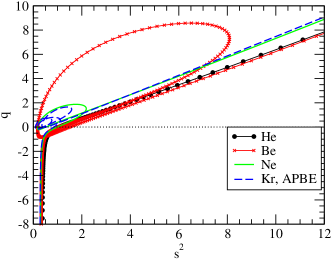
Figure 1: (color online) The parameter space of the combined gradient expansion parameters $s^{2}$ and $q$. Shown are the values of $s^{2}$ and $q$ typically accessed by physical systems – represented here by the He, Be and Ne atoms. The curves show parametric plots of $s^{2}(r)$ versus $q(r)$ each a function of radial position $r$. Black with circles is He, red with crosses is Be, green is Ne, blue dashed is Kr.

The topology of the “phase diagram” of Be is nearly identical to that of He, except for a large loop through the positive $s^{2}$ and $q$ quadrant that coincides with the inter-shell region between core and valence shells. For Ne and Kr, the trend remains essentially the same. Not surprisingly, every transition between shells leads to an extra loop, three for Kr and one for Ne. As predicted from the Thomas-Fermi theory of large-$Z$ atoms, the larger the nuclear charge, the closer the atom approaches globally the slowly varying limit of $q$ and $s^{2}\!\ll\!1$, and we thus see the loops get progressively tighter around the origin as the overall $Z$ increases. The behavior near the cusp is essentially universal, as is the asymptotic limit far outside the atom, although the latter is approached at a slightly different rate than for the lighter atoms. It is interesting to note that the loops are bounded at small $q$ (associated with shell peaks) by the asymptotic straight line limit of each atom, while the final $1s$ shell peak for every atom lines up with the asymptotic limit of the He atom.

The upshot for DFT of this topological analysis is that we have two distinct regions, roughly universal in character for atoms, that may be characterized by the limits of our gradient expansion parameter: $x\!\rightarrow\!\infty$ and $x\!\rightarrow\!-\infty$. This is as long as $\alpha\!>\!0$: at least some information on $\nabla^{2}n$ must be included in $x$ in order to detect the latter limit. At the same time, the quantum oscillations associated with inter-shell transitions cause a loop behavior that cannot be mapped to a function of a single variable $x(s^{2},q)$, and so any energy density constructed from such a variable is inherently inexact. But this behavior could potentially be mapped to a general function of $s^{2}$ and $q$. As this function need be able to handle only a small region near $s^{2}\!=\!q\!=\!0$ for larger atoms, it might be handled adequately by the fourth-order gradient expansion, which depends explicitly on $s^{2}$ and $q$. Svendsen and von Barth (6 II)

III Model and Method

III.1 Model of exchange functional

To develop an exchange functional based upon a hybridization of gradient and Laplacian variables, we start with the GGA. Taking the form for PBE exchange, and replacing the GGA inhomogeneity parameter $s^{2}$ with the more general $3x(s^{2},q)$ of Eq. (12), we get the exchange enhancement factor

$$F_{X}[3x(\alpha)]=1+\frac{3\mu x(\alpha)}{1+3\mu x/\kappa(\alpha)}.$$ (24)

The model is parameterized through the parameters $\mu$ and $\kappa(\alpha)$, (the latter, not being naturally “gauge-invariant”, necessarily dependent upon the hybridization factor $\alpha$) and giving rise to the following limit cases:

$$F_{X}(x) \rightarrow 1+3\mu x, \>x\rightarrow 0$$ (25)

$$F_{X}(x) \rightarrow 1+\kappa(\alpha), \>x\rightarrow\pm\infty.$$ (26)

A moment’s notice shows that this form for $F_{X}$ will not do, since it has a pole at finite negative $x$. Because of the electron density cusp, $x$ varies from $0$ to $-\infty$ in the vicinity of the nucleus, guaranteeing that the pole must be encountered. However, simple fixes such as $F_{X}(x)\!=\!1\!+\!3\mu x/\sqrt{1\!+\!(3\mu x/\kappa)^{2}}$, also fail in this region. Cancio, Wagner, and Wood (2012) The issue seems to be the infinite variation in the inhomogeneity parameter $x$ in a minute region of physical space, $r\!<\!a_{0}/Z$. This extreme variation gives rise to problems in the X potential when the divergence and Laplacian operators of Eq. (14) are taken.

To circumvent this issue, we introduce a “renormalized” or regulated inhomogeneity parameter $\bar{x}$:

$$\bar{x}=x\left[1-\exp{\left(\frac{C\kappa}{3\mu x}\right)}(x<0)\right]$$ (27)

Here $\bar{x}$ has a minimum value of $-C\kappa/3\mu$ as $x\!\rightarrow\!-\infty$, and $C$ can then be chosen so that the denominator of the functional does not have a pole for negative $x$. For $x\!>\!0$, we do not need such a regulation – although the GEA parameter tends to $+\infty$ for large radii, it does so over an infinite range and seems to lack the serious instabilities encountered near the cusp.

In the end, we use with the following modified functional form for exchange:

$$F_{X}(x)=1+\frac{3\bar{\mu}(x)\bar{x}}{\sqrt{1+\eta(3\mu\bar{x}/\kappa)+\left(3\mu\bar{x}/\kappa\right)^{2}}}$$ (28)

where $\bar{x}$ is the regulated version of $x$ described by Eq. (27). The renormalization of $\mu$ in the numerator,

$$\bar{\mu}=\mu\left[1-A\exp{(C\kappa/3\mu x)}(x<0)\right],$$ (29)

gives an additional degree of control allowing us to fit a further constraint on the potential at the nucleus. In addition to conventional DFT constraint parameters $\mu$ and $\kappa$, the model uses variational parameters $C$, $A$ and $\eta$ which can be chosen to optimize curvature in the exchange potential. This form has the same behavior as the PBE for $x\!\rightarrow\!0$ and $x\!\rightarrow\!\infty$ limits, and in the $x\!\rightarrow\!-\infty$ limit reduces to

$$1-\frac{(1-A)\kappa C}{\sqrt{1-\eta C+C^{2}}}+O(1/x)$$ (30)

which has the desired form [Eq. (22)] as long as the denominator in the second term is nonzero and real.

III.2 Calculation of energy and potential

As a starting point of our functional development, we focus on functionals that exactly reproduce the limiting behaviors of known GGA’s. The APBE Constantin et al. (2011) and SOGGA Zhao and Truhlar (2008) variants of the PBE are chosen as representative of two extremes of interpretation of conflicting information about DFT constraints. We keep the $\mu$ value of each model and determine values for $\kappa(\alpha)$ by requiring that the new functional reproduce for any $\alpha$ the exchange energy of the original for the Neon atom, representing the small-$Z$, and thus high-inhomogeneity limit. This strategy gives rise to two new models, a modAPBE and a modSOGGA, defined for the hybrid inhomogeneity parameter $x$ with mixing coefficient of $\alpha\!=\!0.2$. A third, SOGGA-q, represents our best attempt at producing a Laplacian-only model. The parameters used to define these models and their GGA equivalents are shown in Table 1.

Model	$\alpha$	$\mu$	$\kappa$	$\eta$	$C$	$A$
LDA		0.0
SOGGA	0.0	$10/81$	0.552	2.0
APBE	0.0	0.26037	0.804	2.0
SOGGA-q	1.0	$10/81$	0.552	2.0	1.00	1.00
ModSOGGA	0.2	$10/81$	1.104	3.0	0.117	0.129
ModAPBE	0.2	0.26037	1.55	3.0	0.252	0.366

Table 1: Parameters used in defining the DFT models discussed in this paper, as defined by Eqs. 12, 27, 28, and 29.

The remaining variables $\eta,C,A$ are used to constrain the potential, $\eta$ in the region outside the nuclear cusp ($r\!>\!a_{0}/Z$), $C$ and $A$ inside. Minimization of the curvature [Eq. (23)] was the primary constraint with additional considerations from the known behavior of the potential at the nucleus. The curvature integral $I$ must in practice be optimized for some test density or densities and for this purpose we use that of the Be atom. The features that we find produce unphysical curvature in the exchange potential of atoms, the nuclear cusp and the exponential tail in the classically forbidden region outside the atom, are basically universal, whereas Be in addition suffers from high levels of inhomogeneity in the core-valence transition that are an additional source of trouble. Optimization of the potential for this case produces nearly optimal results for the other atomic systems we have studied.

As reference data for small atoms, we use exact Kohn-Sham densities and exchange potentials Umrigar and Gonze (1994); Filippi, Gonze, and Umrigar (1996) which are evaluated on a standard logarthmic grid. Exchange energies are also evaluated for larger closed-shell atoms using the APE pseudopotential generator (Oliveira and Nogueira, 2008) in all-electron mode and the APBE exchange-correlation functional. Laplacians and gradients that appear in the exchange potential are evaluated numerically by the method of Bird and White, White and Bird (1994) evaluated on the grid with Lagrange interpolating polynomials. To check numerical calculations, a few were made using Slater-type orbitals for which analytic values for derivatives could be obtained. The errors in numerical derivatives were negligible (relative errors of order $10^{-9}$ for polynomials of order 11 or 13 and standard grids.)

IV Results

IV.1 Optimization of functional parameters

Our first results are the values of the parameters, shown in Table 1, that meet the constraint conditions on energy and potential – matching known GGA’s for large-$Z$ atoms (representative of slowly-varying densities), small-$Z$ atoms (quickly-varying densities), minimizing the curvature integral $I$ to produce a physically reasonable potential at all $r$, and producing a finite exchange potential with zero slope at the nucleus.

Being a gauge-invariant parameter, $\mu$ takes the value of the corresponding GGA whose constraints we are trying to duplicate, $10/81$ for the SOGGA and $0.2604$ for the APBE, independent of the choice of $\alpha$ taken. To satisfy the other constraints proved tricky given the interconnection between parameters within the form given by Eq. (28). The exchange energy depends primarily on the region outside the nucleus and can be decoupled from the parameters $C$ and $A$ that characterize large negative $x$. For any fixed gauge choice $\alpha$, the requirement that our functional reproduce the exact exchange energy of the Ne atom, our large-inhomogeneity constraint, defines a continuum of possible values $\kappa(\eta)$ for the two remaining free parameters. The exchange potential develops unphysical oscillations at the outside edge of the valence shell for $\eta\!<\!2$, which are particularly large for the Be atom. At the same time larger values of $\eta$ lead to problems at the nucleus, moving the limiting value of $F_{X}$ [Eq. (30)] closer to a singularity. There seems to be a conflict in which optimizing the potential for the one region of space comes at the cost of unphysical curvature in the other. A compromise that works for the natural gauge $\alpha\!=\!0.2$ taken from gradient expansion of the exchange hole is to take $\eta\!=\!3$ and $\kappa$ twice the value derived from the local LO bound. This almost perfectly reproduces GGA exchange energies of filled-shell atoms for our modification of both the SOGGA and the APBE GGA’s, while having essentially the same curvature in the Be potential as the optimal case $\eta\!\sim\!5$. This is somewhat of a surprise since $\eta$ was designed to help prevent a pole in $F_{X}$ at the nucleus, while it functions best to remove curvature in the valence shell. Finally, for $\alpha\!=\!1$, the Laplacian-only theory, it was difficult to find a value of $\kappa$ for which one could match the exchange energy of the GGA and retain a reasonable potential; we had to settle for a reasonably smooth potential and an exchange energy that was not much better than the LDA.

The parameters $C$ and $A$ play a leading role for large negative $x$, roughly $r<0.1~{}a_{B}/Z$, and give us variational freedom to minimize curvature in this region and impose an additional constraint on the X potential at the nucleus – for example the zero slope of the potential observed in numerical data. Filippi, Gonze, and Umrigar (1996); Almbladh and Pedroza (1984) However the minimum curvature in the potential in this region is achieved by introducing a pole in the energy density and potential at the nucleus – the constant $a$ in Eq. (22) tends to infinity as the curvature is minimized. We retain the singularity of the GGA potential, while adding a new singularity in the energy density! The strength of the pole decreases if $\eta$ is reduced, putting curvature back in the large $r$ limit, but it occurs at any value of $\eta$, $\mu$ or $\kappa$ other than zero. Nevertheless, as shown below, this pole can be avoided by accepting a modicum of unphysical curvature in the potential at finite radius. Within the limitations of our current form for $F_{X}$, competition between incompatible constraints limits our ability to meet all our goals for the exchange potential at the nucleus.

Figs. 2 and 3 display some of the features of the enhancement factor introduced in this paper. Fig. 2 shows the “regulated” gradient expansion variable $\bar{x}(x)$ and the ratio of “regulated” to unregulated gradient coefficients $\bar{\mu}(x)/\mu$, both used in $F_{X}$ [Eq. (28)] to optimize its form near the nucleus. The former is equal to $x$ for $x\!>\!0$ but saturates to a finite value for large $x\!<\!0$, thus avoiding a pole in $F_{X}$. The latter shows a renormalization of the gradient coefficient $\mu$ to $\mu(1\!-\!A)$ for large $x\!<\!0$.

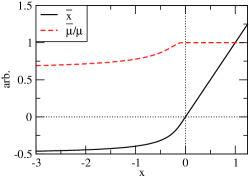
Figure 2: (color online) Regularized gradient expansion variable $\bar{x}$ (black) and linear coefficient $\bar{\mu}$ divided by $\mu$ (red, dashed), for the modAPBE functional.

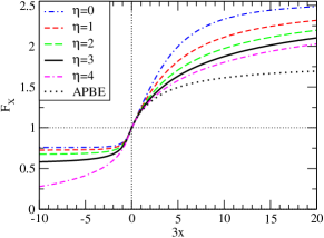
Figure 3: (color online) The enhancement factor $F_{X}$ for the modAPBE functional, as a function of gradient expansion parameter $3x$, for several values of curvature parameter $\eta$, with the other parameters fixed. Solid line shows optimal value of $\eta$. Dotted line is $F_{X}$ for the APBE GGA.

Fig. 3 shows the resulting enhancement factor $F_{X}(x)$ versus $3x$ for the modAPBE, for several values of the potential optimization parameter $\eta$ and in comparison, the enhancement factor for the APBE. (Note that $3x$ maps to $s^{2}$ if the mixing parameter $\alpha$ is turned off.) All the forms have the same linear correction $\mu$ and are thus identical at small $x$. The maximum possible value of $F_{X}$ for the modAPBE is $1\!+\!\kappa\!=\!2.55$, larger than that of the APBE, and compensates for the “dis-enhancement” of the exchange energy that occurs for negative $x$. The regulating effects of using $\bar{x}(x)$ as a variable are seen in the more rapid saturation of $F_{X}$ for negative values of $x$ than for positive, and notably in the absence of a pole in $F_{X}$ for any value of $x$. The enhancement factors with smaller values of $\eta$ have a more kinked form at large $x$, with a larger first derivative, and thus greater curvature $I$. The smoothest forms ($\eta\!\sim\!5$ for the modAPBE) cause an unrealistic positive $\epsilon_{X}$ at the nucleus, while the chosen value $\eta\!=\!3$ gives a nearly correct value for $\epsilon_{X}(0)$ for He.

IV.2 Energies

Figure 4 shows the relative error of the exchange energy with respect to the essentially exact optimized potential method (OPM) Engel and Vosko (3 II); Kurth, Perdew, and Blaha (1999) for filled shelled atoms from He to Rn. Shown are the results for the LDA, the PBE and APBE forms of the GGA, the modAPBE defined in this paper and finally the modified gradient expansion approximation model (mGEA) of Ref. Elliott and Burke, 2009. All energies are calculated with the non-relativistic Schrodinger equation so as to highlight the large-$Z$ scaling limit of Thomas-Fermi theory. The energies for the mGEA and modAPBE functionals are calculated using the APBE density; all others are determined self-consistently. We estimate the use of non-consistent densities to have a very small effect. For example, the PBE exchange energy using the OPM-derived charge densities Engel and Vosko (3 II) is 0.03-0.05% off from that using self-consistent densities.

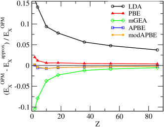
Figure 4: (color online) Fractional error in exchange energy of closed shell atoms for various DFT approximations, relative to optimized potential method (OPM) values, Engel and Vosko (3 II); Kurth, Perdew, and Blaha (1999) plotted versus nuclear charge $Z$.

Perhaps the most interesting data here is that of the mGEA, which uses the gradient expansion enhancement factor

$$F_{X}(s^{2})=1+\mu s^{2}$$ (31)

with the value of $\mu\!=\!0.26037$ obtained by fitting the gradient expansion to the asymptotic large-$Z$ limit of the exchange energy of atoms. Within the extended Thomas-Fermi model of the atom, the LDA value for the exchange energy scales as $Z^{5/3}$ with nuclear charge $Z$, while the GEA correction scales as $Z$, and the next higher term as $Z^{2/3}$. Thus, the relative error in the LDA should decrease as $Z^{-2/3}$ as $Z\!\rightarrow\!\infty$ and the relative error in the GEA, even faster, as $Z^{-1}$. This trend is clearly seen in Fig. 4 – the LDA undershoots the magnitude of the exchange energy for He by about 16%, but declines to 3% for $Z\!=\!86$. This error is essentially eliminated for large $Z$ by the gradient expansion with the mGEA value for $\mu$. If one uses the “traditional” value, $\mu\!=\!10/81$, determined from perturbation theory about the HEG, only half of the LDA error gets removed.

The main error of the mGEA, the poor treatment of the large-$s^{2}$ corrections in the asymptotic region of the atom, primarily affects the smaller $Z$ atoms, since this region constitutes a portion of the total charge density – the tail of the valence shell – that decreases as $1/Z$ as $Z\!\rightarrow\!\infty$. The mGEA systematically overshoots the OPM in magnitude, consistent with a lack of attention to the Lieb-Oxford bound in the GEA form, with gradient corrections unbound from below as $r\!\rightarrow\!\infty$, as shown in Fig. 5(b). The correction of this failure at large $s^{2}$ or small-$Z$ is the key improvement of GGA exchange over the gradient expansion. Both GGA’s shown, the PBE and the APBE, improve dramatically upon the GEA in the low-$Z$ limit. The PBE with $\mu\!=\!0.2195$ is not quite as good a fit as the APBE, which has the same Lieb-Oxford bound limit $\kappa$, but the larger mGEA value of $\mu$. The APBE wins out especially at large $Z$, where it has half the error of the PBE.

The modAPBE introduced here has the mGEA value of $\mu$ and a value of $\kappa$ (=1.55) adjusted to fit the APBE exchange energy for He and Ne. With these constraints, it duplicates the trend in exchange energy for the APBE for all atoms with perhaps a slight degradation in the percent error at high $Z$. This suggests that the physics of the exchange energy of closed shell-atoms is fairly simple and almost completely determined by GGA constraints. And once we determine the right set of constraints to use – ones that are invariant with the choice of energy density gauge – the density functional parameter used to implement them becomes largely irrelevant.

The GEA form as applied to our hybrid parameter $x$ is $F_{X}(x)\!=\!1\!+\!3\mu x$ and by construction should give identical exchange energies regardless of the choice of $\alpha$ in Eq. (27), given the interchangeability of the gradient and Laplacian variables to this order in the gradient expansion. It should also give identical exchange potentials, despite the very different equations used to generate gradient and Laplacian contributions to the overall potential [Eq. (14)]. We have verified this for the mGEA energy using the $\alpha\!=\!0$ ($s^{2}$ only) and $\alpha\!=\!1$ ($q$ only) gauges and APBE charge densities. Both energies and potentials are indistinguishable up to numerical error (7 to 11 significant figures), providing an excellent check for the numerical methods used to calculate them.

Table 2 shows the exchange energy, the value of the exchange potential near $r\!=\!0$, and the curvature integral $I$ [Eq. (23)] for some of the DFT models we have discussed so far. The SOGGA and APBE define weak and strong GGA corrections to the LDA respectively, the modSOGGA and modAPBE are functionals designed to reproduce these GGA’s for atomic systems, and the SOGGA-q is our best Laplacian-only model. The calculations are performed for exact Kohn-Sham densities Umrigar and Gonze (1994); Filippi, Gonze, and Umrigar (1996) and compared to exact exchange potentials.Filippi, Gonze, and Umrigar (1996)

Atom	Model	$E_{x}$	$V_{x}(0)$	$I$
He	LDA	-0.883	-1.509
	SOGGA	-0.961	-14.88
	APBE	-1.02995	-28.77
	SOGGA-q	-0.9017	-9.966	1.5e-03
	modSOGGA	-0.9599	-2.409	1.87e-04
	modAPBE	-1.0280	-5.52	4.52e-04
	KS	-1.02457	-1.688
Be	LDA	-2.321	-3.230
	SOGGA	-2.513	-98.37
	APBE	-2.688	-198.0
	SOGGA-q	-2.368	-25.	1.5e-1
	modSOGGA	-2.512	-5.48	2.7e-3
	modAPBE	-2.6844	-13.2	9.4e-3
	KS	-2.674	-3.126
Ne	LDA	-11.021	-8.391
	SOGGA	-11.621	-238.4
	APBE	-12.209	-480.3
	SOGGA-q	-11.334	-70.	1.5e-3
	modSOGGA	-11.623	-14.8	2.22e-04
	modAPBE	-12.2079	-36.5	5.38e-04
	KS		-7.984
	HF	-12.11

Table 2: Exchange energy, potential at the nucleus, curvature integral for GGA’s and Laplacian-based models (in hartrees), evaluated using exact Kohn-Sham densities. Umrigar and Gonze (1994); Filippi, Gonze, and Umrigar (1996) KS are corresponding results from exact Kohn-Sham density functional theory, and HF from exact Hartree-Fock calculations.Clementi and Roetti (1974)

The SOGGA-q uses the local LO bound value for $\kappa$, but with an energy density gauge ($\alpha\!=\!1)$ quite different from that of a GGA ($\alpha\!=\!0$). The result is a much smaller exchange energy than the SOGGA, close to the LDA, and shows the effect of uncritically using for one gauge of the energy density a constraint defined with respect to another. For the two modGGA functionals, the exchange energy of the respective gradient-only GGA has been matched by doubling the large-inhomogeneity parameter $\kappa$. For the curvature integral $I$, a value $\sim 1\times 10^{-4}$ indicates a potential which is a monotonic convex function, as expected for the X potential for He. The SOGGA-q potential for He is thus not quite optimal but the modAPBE and modSOGGA ones are stable and free of spurious oscillations as indicated by their low $I$. Given the definition of $I$, [Eq. (23)], it is natural that as the $q$ component of the inhomogeneity variable $x$ is turned on, $I$ becomes larger, so that it is consistently at least an order magnitude higher for the SOGGA-q model with $\alpha\!=\!1$ as compared to the modSOGGA with $\alpha\!=\!0.2$. The higher values of $I$ for Be are physically relevant as will be shown below.

The value of the X potential shown in Table 2 is not exactly for $r\!=\!0$, but rather the smallest radius ($\sim 10^{-3}/Z$) in the numerical grid used to defined the atomic density. The value of $V_{X}(0)$ in hartrees obtained from the exact Kohn-Sham calculations varies with $Z$ approximately as $-0.8Z$. The GGA’s evaluated at this radius are well on their way to $-\infty$ while the cusp-corrected modifications of the GGA are clearly finite but lower than the exact values. The best case scenario is the modSOGGA for which $V_{X}(0)$ varies roughly as $-1.4Z$. The stronger gradient correction used by the APBE and modAPBE leads to worse behavior at small $r$: the APBE singularity is more noticeable than that of the SOGGA and the modAPBE $V_{X}(0)$ is almost five times deeper than the exact value.

IV.3 He atom

Fig. 5(a) shows logarithms of the density and the gradient-expansion parameters $s^{2}$, $3q$, and $3x$, as a function of radial distance for the He atom. The density is approximately exponential, leading to a straight line for its logarithm. The parameter $s^{2}$ for an exponential is also exponential and its logarithm increases linearly from a value of $0.18$ near the nucleus. The variables derived from the Laplacian, $3q$ and $3x$, are more complex, since the Laplacian changes sign at $r\sim a_{0}/Z$ and diverges to $-\infty$ near the nucleus.

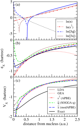
Figure 5: (color online) GEA Density functional parameters (a), exchange energy-per-particle (b), exchange potential (c) for the He atom, as function of distance from the nucleus. In (a), the logarithms of the density (dotted), GEA parameter $s^{2}$ (dash-dotted) the absolute value of $3q$ (dark solid line for $q\!>\!0$ and dashed for $q\!<\!0$) and the hybrid parameter $3x$ (light solid and dashed) are plotted. In (b) and (c), quantities are derived from the LDA (light solid), the mGEA Elliott and Burke (2009) (dotted) the APBE GGA Constantin et al. (2011) (dot-dashed), two functionals defined in the text – the SOGGA-q using the Laplacian variable $q$ (dashed), the modAPBE using the variable $x$. These are compared to numerical values for the exact integral expressions for $V_{X}$ and $\epsilon_{X}$ (dark solid). All quantities are determined using the charge density of Ref. Umrigar and Gonze, 1994.

The parameter $s^{2}$ is defined so that a value appreciably less than one (zero on the log plot) indicates a region of slowly-varying density for which the GEA presumably should be valid. Based on this, one might expect the GEA to be valid for all positions within a scaled Bohr radius $a_{0}/Z$ and gradually diverge from the correct result at large $r$. The Laplacian-based equivalent to $s^{2}$, $3q$, diverges both at the nuclear cusp and in the asymptotic limit and thus is a more accurate indicator of where the GEA fails. The hybrid GEA parameter $3x$ represents a compromise between the two cases. It is quite noticeably close to the $s^{2}$ measure almost everywhere, a consequence of the small value of $\alpha$ that comes from the Becke exchange-hole analysis. However, it diverges at the nucleus, so that it holds true to the correct physics in this region.

Figs. 5(b) and (c) show the exchange energy-per-particle and potential of the He atom as a function of distance from the nucleus, using several of the density functional theories discussed in this paper. These include the LDA, the mGEA, the APBE, presumably the most accurate conventional GGA for atomic systems, and two models based on the Laplacian of the density: the SOGGA-q, using the regularized Laplacian factor $3\bar{q}$ and the modAPBE, using the regularized hybrid of gradient and Laplacian, $3\bar{x}$. For this system, exact values of $\epsilon_{X}$ and $V_{X}$ may be easily obtained given that the exchange energy for a two-electron singlet is simply the removal of the self-interaction energy of each electron and is obtainable from the Hartree potential. A value of $\epsilon_{X}({\bf r})\!=\!-V_{H}({\bf r})/4\!=\!-\int\;n({\bf r}^{\prime})/4\left|{\bf r}-{\bf r}^{\prime}\right|d^{3}r^{\prime}$ obtains this result. (This is not a unique definition of $\epsilon_{X}$ of course, but is directly derived from the exchange hole of the spin singlet, and thus the definition we will be interested in.) Likewise, the potential $V_{X}$, shown in (c), is equal to $-V_{H}/2$. As before, we use the exact Kohn-Sham density for He for this purpose. Umrigar and Gonze (1994)

The LDA is a not unreasonable ballpark result for $\epsilon_{X}$, but it has qualitatively wrong behavior (a cusp) at the nucleus and is shifted upwards from the $-1/2r$ limiting behavior of the true $\epsilon_{X}$. The mGEA improves upon the LDA at high density; far from the nucleus, where $s^{2}$ diverges, it deviates severely from the correct behavior. The conventional GGA, because of its adherence to the local Lieb-Oxford bound, corrects this extreme behavior to provide a reasonable global improvement to the LDA energy-per-particle and energy. Of the three GGA-type models, gratifyingly it is the modAPBE, the hybrid gradient-Laplacian model designed to come as close as possible to the energy of the XC hole, that most closely adheres to the exact values for $\epsilon_{X}$. It does so quite closely for the intermediate distances from the nucleus which contribute most to the total energy. As $r\!\rightarrow\!\infty$, it decays exponentially like the LDA and GGA, but at a slower rate.

Fig. 5(b) reveals why the exchange energy for the SOGGA-q fails to match that of the SOGGA in Table 2 and illustrates the need for treating $\kappa$ as a function of the energy-density gauge $\alpha$. DFT models that rely on $\nabla^{2}n$ have higher energy density than the LDA near the nucleus where $\nabla^{2}n<0$; in contrast GGA’s have a lower energy density. To match the GGA integrated exchange energy, it is then necessary to lower the energy density elsewhere – specifically in the asymptotic large-$r$ region. This is a region of high inhomogeneity where the LO bound kicks in and prevents the energy density from being lowered. Unless it is ignored, the exchange energy of a modGGA cannot be made to match that of the corresponding GGA, but must necessarily be too high.

In Fig. 5(c) are shown the He exchange potentials for the models discussed in Fig. 5(b). The exact model is cuspless and has an asymptotic limit of $-1/r$, and is otherwise largely featureless. The LDA exchange potential is proportional to $n^{1/3}$ and thus has a cusp at $r\!=\!0$ and decays exponentially at large $r$. The result is the well-known, Jones and Gunnarsson (1989) roughly constant shift upwards in energy of the LDA with respect to the exact potential. The various gradient-correction models adhere closely to the LDA at intermediate distances, diverge slightly from it at large distance and slope sharply downwards at the nucleus. The GEA diverges to positive infinity at very large distances. The modAPBE, although it produces a very accurate fit to $\epsilon_{XC}$, produces a potential that is not noticeably different from the APBE from which it is derived.

Fig. 6 shows the behavior of the DFT potentials shown in Fig. 5(c) in the immediate vicinity of the nucleus. The pole in the GGA potential occurs in the “deep cusp” region: $r\!\leq\!0.05a_{0}$ for He, and roughly $r\!\leq\!0.10a_{0}/Z$ in general. The SOGGA GGA, a weaker correction to the LDA, is understandably better behaved than the more aggressive APBE. The corresponding modSOGGA and modAPBE potentials are shown as dashed lines, and show the benefit of including the Laplacian of the density. The modSOGGA is finite at the nucleus with a quite reasonable value for $V_{X}(0)$ and is explicitly cusp-free like the true potential. The modAPBE, though finite at the nucleus, is much further from the true potential, at best marginally better than the corresponding GGA. In both cases, the problem of an unphysical potential at the nucleus does not disappear as much as change form – the pole created by the GGA spreading out spatially into an unphysical dip.

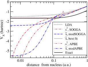
Figure 6: (color online) X potentials for the He atom at the nuclear cusp. Dotted is LDA, exact is black solid, SOGGA GGAZhao and Truhlar (2008) is double-dot-dashed, APBE GGA Constantin et al. (2011) is dot-dashed, modSOGGA long-dashed, modAPBE is short-dashed. Finally a version of the modSOGGA optimized to reproduce the exact potential at the nucleus is shown as grey solid line (brown online).

The consequence of conflicting optimization strategies for the cusp region – either to minimize the curvature or fit the potential at $r\!=\!0$ is demonstrated by a model (grey, brown online) in which the cusp correction parameters are chosen to provide a best fit to the exact X potential in the vicinity of the nucleus. This very close fit comes at a cost of a large fluctuation in the potential, of order a rydberg in energy, in the region where the regularized variable $\bar{x}$ approaches zero. Conversely, completely minimizing curvature comes at the cost of creating a pole at $r\!=\!0$, one which is in fact worse than the corresponding GGA pole. The optimal curve shown in the figure is thus a somewhat arbitrary balance between these two competing effects – minimizing the magnitude of $V_{X}(0)$ while keeping the slope in $V_{X}$ nonnegative for $r\!>\!0$.

IV.4 Beryllium and Neon

Systems of considerably more interest than He are those of Ne. shown in Fig. 7 and Be, shown in Fig. 8. These are the smallest closed-shell atoms that contain the topological feature of a transition between two shells. As shown in Fig. 1, the sequence He, Ne, Be represents a progressive increase of inhomogeneity in the atom interior due to the inter-shell transition, characterized by the growth in the region of $(s^{2},q)$ parameter space probed by each successive system. In Figs. 7 and 8 we show the logarithm of the density, $s^{2}$, and the absolute values of $3q$ and $3x$ in (a); we show exchange potentials in (b).

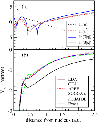
Figure 7: (color online) GEA Density functional parameters (a), and exchange potential (b) for the Ne atom, as function of distance from the nucleus. Quantities plotted are the same as for Fig. 5(a) and (c).

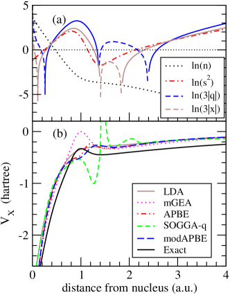
Figure 8: (color online) GEA Density functional parameters (a), and exchange potential (b) for the Be atom, as function of distance from the nucleus. Quantities plotted are the same as for Fig. 5(a) and (c).

In each case, the Laplacian-derived parameter $3q$ is a reliable indicator of shell structure – it is negative at the nuclear cusp and at the peak of the valence shell (shown as the dashed portions of the curve in each figure) and positive in the transitional region between shells and asymptotically. The transition between shells is also indicated by an abrupt change in slope in $ln(n)$, which coincides with a maximum in $\nabla^{2}n$ and $3q$. The gradient-derived $s^{2}$ is less sensitive to structural details, but does exhibit an oscillation at the core-valence boundary. The hybrid parameter $3x$ retains the negative singularity at the cusp exhibited by $3q$ but a has much diminished region of negative value at the valence shell peak, which vanishes altogether for Ne.

With a completely filled valence shell, the transition between the core and valence densities in Ne is fairly gradual and as a consequence, the inhomogeneity parameters $s^{2}$, $3q$, and $3x$ are not too far from the GEA limit in the inter-shell region. For Be, a combination of low net valence charge and a large change in the decay rate of the density makes the core-valence transition one of severe inhomogeneity, with $3q$ topping a value of 24 and $s^{2}$ a value of 8, both well beyond the gradient expansion criterion of $3x\!\ll\!1$. Thus Be is a particularly good stress test for the behavior of density functionals with respect to severely rapid change in density.

Exchange potentials for the DFT models considered in Table 2 are shown for Ne in Fig. 7(b) and Be in Fig. 8(b). The exact potential, like in He, proves hard to match – it lies consistently below that of all DFT potentials, and has an oscillation at the core-valence transition not captured by the DFT models. The LDA faithfully follows the general trend of this potential but, as for He, shifted upwards by roughly a constant amount. The mGEA gives the best qualitative fit of the inter-shell region, at the price of catastrophic failure at large $r$. The imposition of a bound on the X functional for the large-inhomogeneity limit in the APBE and the two mod-GGA’s overcorrects the GEA potential in the inter-shell region, leading to a less accurate result here.

The effects of increasing inhomogeneity as one goes from He to Ne to Be bring about some surprising results, particularly for the SOGGA-q model that depends solely on $q$, the Laplacian-derived GEA variable. The moderately large inhomogeneity encountered in Ne at the core-valence boundary induces oscillatory behavior in the SOGGA-q model that is significantly larger than that of the APBE or modAPBE. This does indicate that the Laplacian is more sensitive to structural details than the gradient of the density – unfortunately the change in potential is in the wrong direction. A more unpleasant surprise occurs with the more inhomogeneous Be atom: huge oscillations appear in the potential, associated with the change in sign in $q$ at $r\!=\!1.4$. Apparently the potential has a nonlinear sensitivity to rapid changes in $q$ that was not apparent for the He atom.

The mGEA, APBE and modAPBE also show a similar, if less dramatic dependence on the inhomogeneity in the transition region, with trends for Ne for each case exaggerated in Be. In the more homogeneous Ne atom, there is very little difference between the three models, a reflection of the relative closeness between the variables $s^{2}$ and $3x$, and their lying largely within the gradient expansion limit. The differences between models are larger for Be, and lead to larger errors with respect to the exact potential. The additional oscillatory structure, genuine or spurious, in the potentials for Ne and Be show up in the curvature $I$ shown in Table 2. Those for Ne are not much larger than for He, but the considerable additional structure for Be causes an order of magnitude jump in this integral.

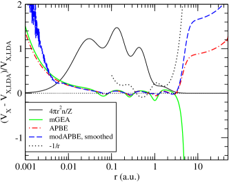
Figure 9: (color online) X potentials for the Kr atom, obtained for the APBE density using the APE pseudopotential generator. Green solid lines shows the mGEA model, red dot-dashed line shows the APBE using the conventional $s^{2}$ GEA parameter, blue dashed line shows the modAPBE using the hybrid GEA parameter $x$, black dotted line shows asymptotic behavior of true exchange potential. Noise in modAPBE data is due to round-off error. An arbitrarily scaled radial density profile (black solid) is included as a guide to the eye.

IV.5 Large atoms

The exchange potential for a typical larger-$Z$ closed-shell atom, Krypton, is shown in Fig. 9. This figure shows the relative difference between several gradient-expansion-derived exchange potentials and that of the LDA. These are calculated from a standard all-electron calculation using the APE pseudopotential generator, (Oliveira and Nogueira, 2008) using the APBE model of exchange and correlation. As a guide to interpretation, the radial probability density for Kr is shown in black at an arbitrary scale, showing clearly the four filled shells of this atom.

All the gradient-corrected potentials are very close to each other, and to the LDA, in the Thomas-Fermi scaling region – for distances outside the nuclear cusp $r\!>\!a_{0}/Z$ up to the asymptotic edge of the valence shell at $r\!\sim\!4~{}a_{0}$. In this region, where the large proportion of electron density is located, the GEA is a good approximation and there is no appreciable difference between GEA, GGA or modGGA. Three dips in the GEA curve, indicating a slightly larger disagreement with the LDA, mark the transitions between the four energy shells and thus intermittent departures from pure scaling behavior.

Plotted as a relative difference with the LDA, the correct limiting behavior of the X potential of $-1/r$ shows up as a positive exponential curve, which is shown for large $r$ as a dotted line. Note that it produces a roughly constant shift with the LDA for intermediate values of $r$ where the Thomas-Fermi approximation is valid.

The mGEA has a singularity at the nuclear cusp independent of $\alpha$ (in the case of the $\alpha\!=\!1$ or $q$-only limit, this is because the GEA lacks the $1/q$ limiting behavior needed to produce a finite potential.) It also diverges from the LDA value asymptotically in the classically forbidden region of the atom, which like the cusp is not treatable in the semiclassical Thomas-Fermi approach. Here it becomes nonzero and diverges exponentially to $+\infty.$ The APBE is identical to the mGEA in the cusp region, tamps down on its oscillatory behavior between shells and has a reasonable long-range behavior. The modAPBE does slightly better than the APBE in the asymptotic limit, in comparison to the correct power-law behavior, because of the larger value of $\kappa$ used. It is hard to qualify it as better in the cusp regime because of excessive numerical noise that appears in taking numerical derivatives for $\nabla^{2}n$ and $V_{X}$. This noise may be reduced by increasing the precision of the the numerical density data used to generate the potential, typically to fifteen significant figures. Nevertheless, it points to a difficulty in implementing our approach – numerical techniques adequate for gradient-based models may not work for Laplacian-based models without retuning. Jemmer and Knowles (1995)

V Discussion

V.1 Future steps

Our functionals are currently limited by a lack of significant information beyond that of the GGA. They are identical to the GGA in the gradient expansion limit and have the same scaling constraints. The large inhomogeneity limit is determined by a fit to the GGA for low-$Z$ atoms. Since they encode the same physics, it is not surprising that our new models closely match the GGA in calculated energies and potentials. The significant difference is tied to the genuinely new piece of physics we have introduced – the behavior of the exchange hole near the nucleus, and thus the behavior of the exchange potential in this region.

It is possible to do better. A next step in DFT development, taken normally in the development of meta-GGA’s, is to satisfy the next-highest or fourth-order term in the gradient expansion for exchange. This involves Laplacians and gradients of the density in a way that cannot be trivially unentangled by an integration by parts. Ignoring the issue of whether that expansion is better derived from the extended Thomas-Fermi theory of the atom or from the homogenous electron gas, the fourth-order gradient expansion about the latter is: (Svendsen and von Barth, 6 II)

$$F^{GEA}_{X}(s^{2},q)=1+\frac{10}{81}3x+\frac{146}{2025}q^{2}+\frac{73}{405}s^{2}q+Ds^{4}$$ (32)

where $D$ is believed to be 0, and $3x$ is the arbitrary linear combination of $s^{2}$ and $q$ of Eq. (12). As we already use the explicit linear combination of $s^{2}$ and $q$ to describe the lowest order correction of the gradient expansion, we automatically generate terms of the correct sort for the higher-order corrections as well. In fact, if we take the choice $3x\!=\!0.6q\!+\!0.8s^{2}$ derived from the gradient expansion of the X hole we can come remarkably close to the fourth-order correction with

$$F^{modGEA}_{X}(x)=1+\frac{10}{81}3x+\frac{1}{5}(3x)^{2},$$ (33)

with a difference $\Delta F_{X}$ from the exact value of

$$\Delta F_{X}(s^{2},q)=-0.0001q^{2}+0.012s^{2}q+0.128s^{4}.$$ (34)

Here the $s^{2}q$ coefficient is within 10% of the exact value; the nonzero value for $D$ is close to that used in a previous metaGGA. Perdew et al. (1999) This nice result is all the more surprising in that the arguments we have used in generating our choice for $x$ are strictly related to the lowest order in perturbation theory.

In our current form for $F_{X}$ [Eq. (28)] there is a free parameter $\eta$ that determines the coefficient of $x^{2}$; however it is already used to minimize the curvature of the derivative of the exchange energy density with $\nabla^{2}n$, and cannot also be used to match the correct fourth-order correction. In fact, the curvature minimization requirement produces a fourth-order gradient correction with the wrong sign, and thus wrong qualitative results. This may be the reason why our X potential seems to be slightly worse than the GGA in the core-valence transition region of Be as shown in Fig. 8.

A necessary further step will be to construct a correlation functional to match the exchange functional introduced here. The goal is to model a structure of the form PBE

$$H_{C}\sim\log\{1+(\beta/\gamma)t^{2}F_{C}[A(r_{s})t^{2}]\}$$ (35)

where $F_{C}$ is an enhancement factor similar to that used for exchange, $A(r_{s})$ a function and $\gamma$ a parameter both fixed by scaling constraints, $\beta$ defines the strength of the gradient correction in the low inhomogeneity limits, and $t^{2}\sim s^{2}/r_{s}$ is the measure of inhomogeneity given by Eq. (7). The minimum step needed to generate a useful correlation functional is to replace $s^{2}$ with the regularized hybrid variable $3\bar{x}$ and use variational techniques to control the resulting potential. A complicating issue is the stringent constraint necessary to have a physically reasonable energy density – the argument to the logarithm must be greater than zero, which is harder to achieve for negative $x$ than the absence of a pole in $F_{C}$. Secondly constraints that would add value to the functional beyond that of the GGA are unknown. What is nature of correlation potential or energy in the limit of large negative $x$, i.e. at the nucleus? What is the correct response to the fourth order gradient expansion for exchange? Do problems with gauge-variant constraints occur – e.g. the limit of large $t^{2}$?

V.2 Conclusions

The major findings of this project have been the greater understanding of the physics behind the generalized gradient approximation of DFT. We have shown that in principle, a GGA good for a large range of systems and conditions can be constructed starting from any linear combination of $\left|\nabla n\right|^{2}$ and $\nabla^{2}n$ that produces the same gradient expansion correction, giving rise to an infinite family of “gauge choices” parameterized by a linear coefficient $\alpha$, from $\alpha\!=\!0$, or gradient only, to $\alpha\!=\!1$, or Laplacian only. This model then fits all constraints that any standard GGA fits, as long as they can be framed in a specifically gauge-invariant way. This result gives the DFT development community a greater degree of flexibility in constructing future DFT’s.

We have found some fundamental differences between gauge choices, however, and with them, some important caveats to the finding above. The two extremes $\alpha\!=\!0$ and $\alpha\!=\!1$ each have important defects which lead to failure when the result of the gradient expansion limit is extended to all density-functional space. The gradient-only limit fails at the nucleus, with a spurious singularity in the potential, but this problem likely has a small effect for most atoms. The Laplacian-only limit is plagued by spurious oscillations in the potential that we have been unable to control to a reasonable degree. And these occur in places, such as the valence shell of atoms, or the transition between shells, where these problems cannot be ignored. Thus the $\alpha\!=\!1$ case that we have explored must be considered the worse choice.

However hybrids work. Just like hybrids in other areas of science, or, for that matter, in other areas of density functional theory, the combination of two alternate formulations of a problem lead to formulation that is superior to both. A choice of $\alpha\!=\!0.2$, inspired by a gradient expansion of the exchange hole, cures the problems of both conventional GGA and our exploratory Laplacian-based approach, thus providing the best of both worlds. This supports the philosophy of DFT development based on modeling the XC hole that was the original inspiration for this work – it is in paying attention to the XC hole that an optimal hybrid solution is derived.

The technique of eliminating false oscillations in the exchange potential by the minimization of the curvature of $\partial e_{XC}/\partial\nabla^{2}n$ is a useful technical advance. It is the key here to finding a successful functional form that includes $\nabla^{2}n$ and produces consistently stable and reliable potentials over a wide variety of systems. It may seem that our hybrid-variable functional is so close a match to the GGA because it is a trivial extension of it. But this obscures the fact that it would certainly have performed worse without the optimization of variational parameters $\eta$ and $C$. And the final choices made for these parameters were very much unexpected. In other words, it is only after a “hidden constraint” that the X potential should be as free of unphysical curvature as possible that the connection between the Laplacian-based GGA and conventional GGA becomes evident. Such a technique should prove useful in future attempts to produce workable models for orbital-free XC or kinetic energy densities.

Not all constraints are what they seem. The local Lieb-Oxford bound that is a key component of conventional GGA’s has had to be rethought. As a constraint on the energy density, and not the energy, it is not a physical constraint and must be altered if one changes the “gauge” of the energy density, say by shifting from density gradient to density Laplacian. The global Lieb-Oxford bound is a true physical constraint, but is a bound and a very loose one in practice, and thus of less value than other constraints in DFT such as scaling laws and limit cases which are exact conditions. An exact physical constraint equivalent to the local Lieb-Oxford bound, one that is generally applicable and exact, is the low-$Z$ limit of atomic exchange energies, with the contrasting constraint of weak inhomogeneity provided by the large-$Z$ limit. This approach matches the LDA to one set of exact physical results (the homogeneous electron gas) and the GGA to another (atomic energies). It reflects the relative importance of the contribution of “surface” of the atom, which requires a GGA correction, to the “volume” where extended Thomas-Fermi theory and hence the gradient expansion is exact.

Much of what one would like to fix in the GGA X potential for atoms – bad treatment of the oscillations at shell boundaries and failure to handle the $1/r$ asymptotic behavior of the true potential, is not fixed by our models. This is due in large part to the essential limitation of our approach as an alternative “gauge” for the GEA: many energetically relevant regions of electronic systems are near the gradient expansion limit, where there is with mathematical certitude no difference between our models and conventional GGA’s. Secondly, where we are not at this limit, it is not obvious that the Laplacian can provide the necessary information to fix the GGA. Semilocal models, those involving only the local density and its derivatives, have the limitation of being tied to the local environment, while real systems, especially in such important cases as the covalent bond, have inherently nonlocal aspects to them. Thus, for example, the inability of all semilocal models to obtain the correct $1/r$ limit of the X potential seems to be inherently a property of self-interaction error that may not be removable except at a higher level of theory. Ultimately, it seems that it is the constraints imposed, once they are defined properly, and once hidden ones such as curvature minimization are identified, that define the performance of the DFT models we have studied. Our model is a net improvement over the GGA not so much because it uses the Laplacian of the density but because it fits constraints at the nucleus that are not satisfiable by the GGA.

Within this context, there is some hope for improvement. The transition region between atomic shells, one of relatively high inhomogeneity, is qualitatively poorly described by GGA potentials, and our more general model does not help. However, this may be due to some degree to the fact that it does not capture the proper fourth-order gradient expansion for the exchange energy. This is quite within the capabilities of our approach to DFT, by generalizing the enhancement factor $F_{X}(x)$ to have the correct $x^{2}$ coefficient while otherwise keeping curvature in the potential to a minimum. A second opportunity is to explore areas of electronic topology that are not accessible with atomic densities. The most important such case would be the chemical bond, particularly the situation of large positive $q$ and zero $s^{2}$ that occurs in a bond as its constituent atoms become dissociated. (Covalent bonds explore negative but small values of $q$ that presumably could be mapped back to a GGA.) The information about electronic topology that the Laplacian could bring to the case of bond dissociation may help improve DFT predictions of bondlengths and molecular potential surfaces.