PT-symmetry Management in Oligomer Systems

Abstract

We study the effects of management of the PT-symmetric part of the potential within the setting of Schrödinger dimer and trimer oligomer systems. This is done by rapidly modulating in time the gain/loss profile. This gives rise to a number of interesting properties of the system, which are explored at the level of an averaged equation approach. Remarkably, this rapid modulation provides for a controllable expansion of the region of exact PT-symmetry, depending on the strength and frequency of the imposed modulation. The resulting averaged models are analyzed theoretically and their exact stationary solutions are translated into time-periodic solutions through the averaging reduction. These are, in turn, compared with the exact periodic solutions of the full non-autonomous PT-symmetry managed problem and very good agreement is found between the two.

I Introduction

It has been about a decade and a half since the radical and highly innovative proposal of C. Bender and his collaborators R1 regarding the potential physical relevance of Hamiltonians respecting Parity (P) and time-reversal (T) symmetries. While earlier work was focused on an implicit postulate of solely self-adjoint Hamiltonian operators, this proposal suggested that these fundamental symmetries may allow for a real operator spectrum within a certain regime of parameters which is regarded as the regime of exact PT-symmetry. On the other hand, beyond a critical parametric strength, the relevant operators may acquire a spectrum encompassing imaginary or even genuinely complex eigenvalues, in which case, we are referring (at the linear level) to the regime of broken PT-phase.

These notions were intensely studied at the quantum mechanical level, chiefly as theoretical constructs. Yet, it was the fundamental realization that optics can enable such “open” systems featuring gain and loss, both at the theoretical Muga ; ziad ; Ramezani ; Kuleshov and even at the experimental dncnat ; salamo level, that propelled this activity into a significant array of new directions, including the possibility of the interplay of nonlinearity with PT-symmetry. In this optical context, the well-known connection of the Maxwell equations with the Schrödinger equation was utilized, and Hamiltonians of the form $H=-(1/2)\Delta+V(x)$ were considered at the linear level with the PT-symmetry necessitating that the potential satisfies the condition $V(x)=V^{\star}(-x)$. Yet another physical context where such systems have been experimentally “engineered” recently is that of electronic circuits; see the work of tsampikos_recent and also the review of tsampikos_review . In parallel to the recent experimental developments, numerous theoretical groups have explored various features of both linear PT-symmetric potentials kot1 ; sukh1 ; kot2 ; grae1 ; grae2 ; kot3 ; pgk ; dmitriev1 ; dmitriev2 ; R30add1 ; R30add2 ; R30add3 ; R30add4 ; R30add5 ; R34 ; R44 ; R46 ; baras1 ; baras2 ; konorecent3 ; leykam ; konous ; djf ; kondark ; uwe ; tyugin ; pickton and even of nonlinear ones such where a PT-symmetric type of gain/loss pattern appears in the nonlinear term miron ; konorecent ; konorecent2 ; meid .

Our aim in the present work is to combine this highly active research theme of PT-symmetry with another topic of considerable recent interest in the physics of optical and also atomic systems, namely that of “management”; see, e.g., Refs. boris_book ; turitsyn_review for recent reviews. Originally, the latter field had a significant impact at the level of providing for robust soliton propagation in suitable regimes of the so-called dispersion/nonlinearity management. More recently, as the above references indicate, the possibility (in both nonlinear optics and atomic physics) of periodic –or other– variation also of the nonlinearity has become a tool of significant value and has enabled to overcome a number of limitations including e.g. the potential of catastrophic collapse of bright solitary waves in higher dimensions. In our PT-symmetric setting, to the best of our knowledge, such a temporal modulation of (just the linear in our case footnote ) gain and loss over time has not been proposed previously. Admittedly, in the optical setting, and over the propagation distance, this type of variation may be harder to achieve. Nevertheless, in an electronic setting where the properties of gain can be temporally controlled by relevant switching devices, such a realization may be deemed as more feasible. Our argument herein is that it is also very worthwhile to consider this problem from the point of view of its implications.

In particular, in what follows, we illustrate that in the case of a rapid modulation (“strong” management boris_book ; turitsyn_review ), it is possible to understand the non-autonomous PT-symmetric system by considering its effective averaged form. We showcase this type of averaging in the case of PT-symmetric oligomers, previously explored in a number of works (see e.g. kot1 ; pgk ; konorecent3 ; tyugin ; pickton ; meid , among others). We examine, more specifically, the case of dimers and trimers kipnew which are the most tractable (also analytically) among the relevant configurations. Our findings suggest that there are interesting features that arise in the averaged models which are, in turn, found to be confirmed by the original non-autonomous ones. For instance, in the case of the dimer, the averaged effective model develops an effective linear coupling (and nonlinear self-interaction) coefficient, which has a dramatic implication in controllably expanding the region of the exact PT-symmetric phase, as a function of the strength and frequency of the associated modulation. Our analysis clearly illustrates how this is a direct consequence of the averaging process, and the properties of the periodic solutions are reconstructed on the basis of the averaging and are favourably compared to the observations of the time-periodic solutions of the original non-autonomous system.

Our presentation is structured as follows. In section II, we systematically develop the averaging procedure both for the dimer and for the trimer; the generalization to more sites will then be evident. In section III, we provide some general insight on the existence and stability of solutions in these effective averaged systems. In section IV, we corroborate these results with numerical simulations of the full non-autonomous dimer/trimer systems, finding very good agreement between the two. Finally, in section V, we summarize our conclusions and comment on some interesting directions for potential future work.

II The Averaged Equations for the PT-symmetric Dimer and Trimer models

II.1 DNLS PT-symmetric Dimer Model

We start by considering the DNLS dimer model with a rapidly-varying gain/loss term of the form:

$$i\frac{du}{dt}=\kappa v+|u|^{2}u+i\gamma_{0}u+\frac{i}{\epsilon}\gamma_{1}(t/\epsilon)u,$$

$$i\frac{dv}{dt}=\kappa u+|v|^{2}v-i\gamma_{0}v-\frac{i}{\epsilon}\gamma_{1}(t/\epsilon)v,$$ (1)

where $t$ is the evolution variable, $\epsilon$ is a small parameter, $\gamma_{0}$ represents the linear gain and loss strength and $\gamma_{1}(t/\epsilon)$ is the rapidly-varying gain/loss profile that will be central to our considerations herein. We now apply a multiple scales analysis to Eq. (II.1) in order to derive an averaged equation for our problem. First, we define the new variables $\tau=t/\epsilon$ (fast scale) and $T=t$ (slow scale), and introduce the the transformations

$$u(t)=U(T,\tau)\exp[\Gamma(\tau)],\qquad v(t)=V(T,\tau)\exp[-\Gamma(\tau)],$$ (2)

where $\Gamma(\tau)=\int_{0}^{\tau}~{}\gamma_{1}(\tau^{\prime})d\tau^{\prime}$. This way, we cast Eqs. (II.1) into the following form:

$$\frac{i}{\epsilon}\frac{\partial U}{\partial\tau}+i\frac{\partial U}{\partial T}=\kappa\exp[-2\Gamma(\tau)]V+\exp[2\Gamma(\tau)]|U|^{2}U+i\gamma_{0}U,$$

$$\frac{i}{\epsilon}\frac{\partial V}{\partial\tau}+i\frac{\partial V}{\partial T}=\kappa\exp[2\Gamma(\tau)]U+\exp[-2\Gamma(\tau)]|V|^{2}V-i\gamma_{0}V.$$ (3)

Next, expanding the unknown fields $U(T,\tau)$ and $V(T,\tau)$ in powers of $\epsilon$, i.e.,

$$U(T,\tau)=\sum_{n=0}^{\infty}~{}\epsilon^{n}U_{n}(T,\tau),\qquad V(T,\tau)=\sum_{n=0}^{\infty}~{}\epsilon^{n}V_{n}(T,\tau),$$ (4)

we derive from Eqs. (II.1) the following results.

At the leading-order of approximation, i.e., at $\mathcal{O}(1/\epsilon)$, we obtain the equations $i\partial U_{0}/\partial\tau=0$ and $i\partial V_{0}/\partial\tau=0$, which suggest that the fields $U_{0}$ and $V_{0}$ depend only on the slow time scale $T$, i.e.,

$$U_{0}(T,\tau)=\tilde{U}_{0}(T),\qquad V_{0}(T,\tau)=\tilde{V}_{0}(T).$$ (5)

Additionally, at the order $\mathcal{O}(1)$, we obtain the following set of equations:

$$i\frac{\partial U_{1}}{\partial\tau} + i\frac{\partial U_{0}}{\partial T}=\kappa\exp[-2\Gamma(\tau)]V_{0}+\exp[2\Gamma(\tau)]|U_{0}|^{2}U_{0}+i\gamma_{0}U_{0},$$

$$i\frac{\partial V_{1}}{\partial\tau} + i\frac{\partial V_{0}}{\partial T}=\kappa\exp[2\Gamma(\tau)]U_{0}+\exp[-2\Gamma(\tau)]|V_{0}|^{2}V_{0}-i\gamma_{0}V_{0}.$$ (6)

Next, using the definition of the average of some function $f(\tau)$ over a period $T$ as $\langle f(\tau)\rangle\equiv(1/T)\int_{0}^{T}~{}f(\tau)d\tau$, we average Eqs. (6) over the period $T_{0}$ of $\gamma_{1}(\tau)$, and obtain the equations:

$$\frac{i}{T_{0}}\int_{0}^{T_{0}}~{}\frac{\partial U_{1}}{\partial\tau}d\tau=\frac{1}{T_{0}}\int_{0}^{T_{0}}~{}d\tau\left[-i\frac{\partial\tilde{U}_{0}}{\partial T}+\kappa\exp[-2\Gamma(\tau)]\tilde{V}_{0}+\exp[2\Gamma(\tau)]|\tilde{U}_{0}|^{2}\tilde{U}_{0}+i\gamma_{0}\tilde{U}_{0}\right]$$

$$\frac{i}{T_{0}}\int_{0}^{T_{0}}~{}\frac{\partial V_{1}}{\partial\tau}d\tau=\frac{1}{T_{0}}\int_{0}^{T_{0}}~{}d\tau\left[-i\frac{\partial\tilde{V}_{0}}{\partial T}+\kappa\exp[2\Gamma(\tau)]\tilde{U}_{0}+\exp[-2\Gamma(\tau)]|\tilde{V}_{0}|^{2}\tilde{V}_{0}-i\gamma_{0}\tilde{V}_{0}\right],$$ (7)

where we have also used the result in Eqs. (5). The solvability condition for these equations is satisfied if derive the following set of averaged equations for $\tilde{U}_{0}(T)$ and $\tilde{V}_{0}(T)$:

$$i\frac{\partial U_{0}}{\partial T}=\kappa_{1}V_{0}+g_{1}|U_{0}|^{2}U_{0}+i\gamma_{0}U_{0},$$

$$i\frac{\partial V_{0}}{\partial T}=\kappa_{2}U_{0}+g_{2}|V_{0}|^{2}V_{0}-i\gamma_{0}V_{0},$$ (8)

where, for convenience, we have dropped the tildes; the (constant) coefficients of the above system are given by:

$$\kappa_{1}\equiv\frac{\kappa}{T_{0}}\int_{0}^{T_{0}}\exp[-2\Gamma(\tau)]d\tau,~{}~{}~{}~{}~{}\kappa_{2}\equiv\frac{\kappa}{T_{0}}\int_{0}^{T_{0}}\exp[2\Gamma(\tau)]d\tau,\hskip 36.135pt$$

$$g_{1}\equiv\frac{1}{T_{0}}\int_{0}^{T_{0}}\exp[2\Gamma(\tau)]d\tau=\frac{\kappa_{2}}{\kappa},~{}~{}~{}~{}~{}g_{2}\equiv\frac{1}{T_{0}}\int_{0}^{T_{0}}\exp[-2\Gamma(\tau)]d\tau=\frac{\kappa_{1}}{\kappa},$$ (9)

and it should be recalled that $\Gamma(\tau)=\int_{0}^{\tau}~{}\gamma_{1}(\tau^{\prime})d\tau^{\prime}$ for some choice of $\gamma_{1}(\tau)$. For example, the choice of $\gamma_{1}(\tau)=\gamma_{1}\cos(\tau)$ allows one to express $\kappa_{1},\kappa_{2},g_{1}~{}\mbox{and}~{}g_{2}$ in terms of modified Bessel functions. In this case, the period $T_{0}=2\pi$ and $\gamma_{1}$ is a constant that controls the amplitude of the temporal modulation.

In the next section, we will follow the method employed above to derive an averaged set of equations for the DNLS PT-symmetric trimer model.

II.2 DNLS PT-symmetric trimer model

We now consider the following DNLS trimer model with a rapidly-varying gain/loss term:

$$i\frac{du}{dt}=-\kappa v-|u|^{2}u-i\gamma_{0}u-\frac{i}{\epsilon}\gamma_{1}(t/\epsilon)u,$$

$$i\frac{dv}{dt}=-\kappa(u+w)-|v|^{2}v,\hskip 36.135pt$$

$$i\frac{dw}{dt}=-\kappa v-|w|^{2}w+i\gamma_{0}w+\frac{i}{\epsilon}\gamma_{1}(t/\epsilon)w,$$ (10)

where we have used the same notation as in the case of the dimer. We again assume that the unknown fields depend on the fast and slow scales $\tau$ and $T$, and can be expressed as:

$$u(t)=U(T,\tau)\exp[\Gamma(\tau)],~{}~{}~{}~{}~{}v(t)=V(T,\tau),~{}~{}~{}~{}~{}w(t)=W(T,\tau)\exp[-\Gamma(\tau)],$$ (11)

where $\Gamma(\tau)=-\int_{0}^{\tau}~{}\gamma_{1}(\tau^{\prime})d\tau^{\prime}$, and $U(T,\tau)$, $V(T,\tau)$ and $W(T,\tau)$ obey the following system:

$$\frac{i}{\epsilon}\frac{\partial U}{\partial\tau}+i\frac{\partial U}{\partial T}=-\kappa\exp[-\Gamma(\tau)]V-\exp[2\Gamma(\tau)]|U|^{2}U-i\gamma_{0}U,$$

$$\frac{i}{\epsilon}\frac{\partial V}{\partial\tau}+i\frac{\partial V}{\partial T}=-\kappa\exp[\Gamma(\tau)]U-\kappa\exp[-\Gamma(\tau)]W-|V|^{2}V,$$

$$\frac{i}{\epsilon}\frac{\partial W}{\partial\tau}+i\frac{\partial W}{\partial T}=-\kappa\exp[\Gamma(\tau)]V-\exp[-2\Gamma(\tau)]|W|^{2}W+i\gamma_{0}W.$$ (12)

Next, expanding, as before, $U(T,\tau)$, $V(T,\tau)$ and $W(T,\tau)$ in powers of $\epsilon$, namely,

$$U(T,\tau)=\sum_{n=0}^{\infty}~{}\epsilon^{n}U_{n}(T,\tau),\qquad V(T,\tau)=\sum_{n=0}^{\infty}~{}\epsilon^{n}V_{n}(T,\tau),\qquad W(T,\tau)=\sum_{n=0}^{\infty}~{}\epsilon^{n}W_{n}(T,\tau),$$ (13)

we obtain from Eqs. (II.2) the following results.

First, at the order $\mathcal{O}(1/\epsilon)$, we obtain the equations $i\partial U_{0}/\partial\tau=0$, $i\partial V_{0}/\partial\tau=0$, and $i\partial W_{0}/\partial\tau=0$, which show that the fields $U_{0}$, $V_{0}$ and $W_{0}$ depend only on the slow time scale $T$, i.e.,

$$U_{0}(T,\tau)=\tilde{U}_{0}(T),\qquad V_{0}(T,\tau)=\tilde{V}_{0}(T),\qquad W_{0}(T,\tau)=\tilde{W}_{0}(T).$$ (14)

Next, at the order $\mathcal{O}(1)$, we obtain the system:

$$i\frac{\partial U_{1}}{\partial\tau}+i\frac{\partial U_{0}}{\partial T}=-\kappa\exp[-\Gamma(\tau)]V_{0}-\exp[2\Gamma(\tau)]|U_{0}|^{2}U_{0}-i\gamma_{0}U_{0},$$

$$i\frac{\partial V_{1}}{\partial\tau}+i\frac{\partial V_{0}}{\partial T}=-\kappa\exp[\Gamma(\tau)]U_{0}-\kappa\exp[-\Gamma(\tau)]W_{0}-|V_{0}|^{2}V_{0},$$

$$i\frac{\partial W_{1}}{\partial\tau}+i\frac{\partial W_{0}}{\partial T}=-\kappa\exp[\Gamma(\tau)]V_{0}-\exp[-2\Gamma(\tau)]|W_{0}|^{2}W_{0}+i\gamma_{0}W_{0}.$$ (15)

Similarly to the case for the PT-symmetric dimer model, we average the above system over the period $T_{0}$ of $\gamma_{1}(\tau)$. Then, employing the solvability conditions for the resulting system, i.e., $U_{1}(T,\tau)$, $V_{1}(T,\tau)$ and $W_{1}(T,\tau)$ are periodic in $\tau$ with period $T_{0}$, we obtain the following set of averaged equations for $\tilde{U}_{0}$, $\tilde{V}_{0}$ and $\tilde{W}_{0}$:

$$i\frac{\partial U_{0}}{\partial T}=-\tilde{\kappa}_{1}V_{0}-g_{1}|U_{0}|^{2}U_{0}-i\gamma_{0}U_{0},$$

$$i\frac{\partial V_{0}}{\partial T}=-\tilde{\kappa}_{2}U_{0}-\tilde{\kappa}_{1}W_{0}-|V_{0}|^{2}V_{0},$$

$$i\frac{\partial W_{0}}{\partial T}=-\tilde{\kappa}_{2}V_{0}-g_{2}|W_{0}|^{2}W_{0}+i\gamma_{0}W_{0},$$ (16)

where, as in the dimer case, tildes have been dropped; the coefficients of the above equations are given by:

$$\tilde{\kappa}_{1}\equiv\frac{\kappa}{T_{0}}\int_{0}^{T_{0}}\exp[-\Gamma(\tau)]d\tau,~{}~{}~{}~{}~{}\tilde{\kappa}_{2}\equiv\frac{\kappa}{T_{0}}\int_{0}^{T_{0}}\exp[\Gamma(\tau)]d\tau$$

$$g_{1}\equiv\frac{1}{T_{0}}\int_{0}^{T_{0}}\exp[2\Gamma(\tau)]d\tau,~{}~{}~{}~{}~{}g_{2}\equiv\frac{1}{T_{0}}\int_{0}^{T_{0}}\exp[-2\Gamma(\tau)]d\tau.$$ (17)

Notice that $g_{1}$ and $g_{2}$ are given by expressions identical to those defined in the previous section. Additionally, we will again consider the case with $\gamma_{1}(\tau)=\gamma_{1}\cos(\tau)$ (with the constant $\gamma_{1}$ being the modulation amplitude).

III Analysis of the Averaged Systems

We will now find solutions of the averaged effective PT dimer and trimer models, and investigate their stability.

III.1 DNLS PT-symmetric dimer model

In the averaged dimer case, we seek stationary solutions in the form:

$$U_{0}(T)=a\exp(-iEt),~{}~{}~{}~{}~{}~{}~{}~{}V_{0}(t)=b\exp(-iEt)$$ (18)

where amplitudes $a,b$ are complex and frequency (or energy) $E$ is real-valued. Moreover, using a polar decomposition for $a$ and $b$ of the form:

$$a=Ae^{i\phi_{a}},~{}~{}~{}~{}~{}~{}b=Be^{i\phi_{b}},$$ (19)

we obtain the following set of real equations for $A$ and $B$:

$$\kappa_{1}B\sin(\Delta\phi)+\gamma_{0}A=0,~{}~{}~{}~{}~{}~{}-\kappa_{2}A\sin(\Delta\phi)-\gamma_{0}B=0$$

$$EA=\kappa_{1}B\cos(\Delta\phi)+g_{1}A^{3},~{}~{}~{}~{}~{}~{}EB=\kappa_{2}A\cos(\Delta\phi)+g_{2}B^{3},$$ (20)

where $\Delta\phi\equiv\phi_{b}-\phi_{a}$. The compatibility condition of the equations containing $\sin(\Delta\phi)$ yields:

$$A^{2}=\frac{\kappa_{1}}{\kappa_{2}}B^{2}.$$ (21)

The above equation is then substituted into the compatibility condition of the equations containing $\cos(\Delta\phi)$, yielding the equation $g_{1}\kappa_{1}=g_{2}\kappa_{2}$; the latter is always satisfied, as seen by Eqs. (II.1). Next, we use standard trigonometric identities to express $A^{2}$ in terms of parameters $\kappa_{1}$, $\kappa_{2},\gamma_{0}~{}\mbox{and}~{}E$; this way, we obtain the algebraic equation $(E-g_{1}A^{2})^{2}+{\gamma_{0}}^{2}=\kappa_{1}\kappa_{2}$, which leads to the result:

$$A^{2}=\frac{E\mp\sqrt{\kappa_{1}\kappa_{2}-{\gamma_{0}}^{2}}}{g_{1}}.$$ (22)

Obviously, $A^{2}$ is real only if $E>\sqrt{\kappa_{1}\kappa_{2}-{\gamma_{0}}^{2}}$ or $E>-\sqrt{\kappa_{1}\kappa_{2}-{\gamma_{0}}^{2}}$, provided that $\kappa_{1}\kappa_{2}-{\gamma_{0}}^{2}~{}>~{}0$. In fact, the latter inequality defines the condition for being in the exact (and not in the broken) PT-symmetric phase.

One can also examine the stability of the stationary solutions found for the PT-symmetric effective dimer case. Particularly, we consider the linearization ansatz on top of the stationary solutions of Eq. (II.1) to have the form:

$$U_{0}(t)=e^{-iEt}[a+pe^{\lambda t}+Pe^{\lambda^{*}t}],~{}~{}~{}~{}~{}V_{0}(t)=e^{-iEt}[b+qe^{\lambda t}+Qe^{\lambda^{*}t}],$$ (23)

where the star denotes complex conjugate. Substituting the above ansatz into Eq. (II.1) and linearizing in $p,P,q~{}\mbox{and}~{}Q$, we obtain the eigenvalue problem:

$${\bf A}{\bf X}=i\lambda{\bf X},$$ (24)

where ${\bf X}=(p,~{}-P^{*},~{}q,~{}-Q^{*})^{T}$ and the $4\times 4$ matrix ${\bf A}$ has elements $a_{ij}$ given by:

$$a_{11}=-E+2g_{1}|a|^{2}+i\gamma_{0}~{}~{}~{}a_{12}=g_{1}a^{2},~{}~{}~{}a_{13}=\kappa_{1},~{}~{}~{}a_{14}=0$$

$$a_{21}=-g_{1}(a^{*})^{2},~{}~{}~{}a_{22}=E-2g_{1}|a|^{2}+i\gamma_{0},~{}~{}~{}a_{23}=0,~{}~{}~{}a_{24}=-\kappa_{1}$$

$$a_{31}=\kappa_{2},~{}~{}~{}a_{32}=0,~{}~{}~{}a_{33}=-E+2g_{2}|b|^{2}-i\gamma_{0},~{}~{}~{}a_{34}=g_{2}b^{2}$$

$$a_{41}=0,~{}~{}~{}a_{42}=-\kappa_{2},~{}~{}~{}a_{43}=-g_{2}(b^{*})^{2},~{}~{}~{}a_{44}=E-2g_{2}|b|^{2}-i\gamma_{0}.$$ (25)

Upon substituting the parameters characterizing the solutions of the PT-symmetric dimer model into $a_{ij}$, and solving the eigenvalue problem (24), one can then find the eigenvalues $\lambda$, which determine the spectral stability of the corresponding nonlinear solutions: the existence of eigenvalues with positive real part, $\lambda_{r}>0$, amounts to a dynamical instability of the relevant solution, while in the case where all the eigenvalues have $\lambda_{r}\leq 0$, the solution is linearly stable. We will offer more details on the specifics of the linearization analysis in the numerical section, for the particular choice of cosinusoidal dependence of $\gamma$ on time considered herein.

III.2 DNLS PT-symmetric trimer model

First, we rewrite Eqs. (II.2) in the following form:

$$i\frac{\partial U_{0}}{\partial t}=k_{1}V_{0}+g_{1}|U_{0}|^{2}U_{0}+i\gamma_{0}U_{0},$$

$$i\frac{\partial V_{0}}{\partial t}=k_{2}U_{0}+k_{1}W_{0}+|V_{0}|^{2}V_{0},$$

$$i\frac{\partial W_{0}}{\partial t}=k_{2}V_{0}+g_{2}|W_{0}|^{2}W_{0}-i\gamma_{0}W_{0}.$$ (26)

where the averaged coefficients $k_{1}\equiv-\tilde{\kappa}_{1}$, $k_{2}\equiv-\tilde{\kappa}_{2}$, $g_{1}~{}\mbox{and}~{}g_{2}$ are given in Eq. (II.2). We again seek stationary solutions of the form:

$$U_{0}(t)=a\exp(-iEt),~{}~{}~{}~{}~{}~{}V_{0}(t)=b\exp(-iEt),~{}~{}~{}~{}~{}~{}W_{0}(t)=c\exp(-iEt)$$ (27)

where $E$ is real-valued and the complex amplitudes $a,b$ and $c$ are decomposed as:

$$a=Ae^{i\phi_{a}},~{}~{}~{}~{}b=Be^{i\phi_{b}},~{}~{}~{}~{}c=Ce^{i\phi_{c}}.$$ (28)

Substituting the above expressions into Eqs. (III.2) we obtain the following system for $A$, $B$ and $C$:

$$k_{1}B\sin(\Delta\phi_{1})+\gamma_{0}A=0,~{}~{}~{}~{}~{}k_{2}B\sin(\Delta\phi_{2})-\gamma_{0}C=0,\hskip 72.26999pt$$

$$EA=k_{1}B\cos(\Delta\phi_{1})+g_{1}A^{3},~{}~{}~{}~{}~{}EC=k_{2}B\cos(\Delta\phi_{2})+g_{2}C^{3},\hskip 57.81621pt$$

$$EB=k_{2}A\cos(\Delta\phi_{1})+k_{1}C\cos(\Delta\phi_{2})+B^{3},~{}~{}~{}~{}~{}-k_{2}A\sin(\Delta\phi_{1})-k_{1}C\sin(\Delta\phi_{2})=0,$$ (29)

where $\Delta\phi_{1}\equiv\phi_{b}-\phi_{a}$ and $\Delta\phi_{2}\equiv\phi_{b}-\phi_{c}$. We determine nontrivial solutions for $A,B$ and $C$ by solving the first four equations in Eq. (III.2) for $\sin(\Delta\phi_{1})$, $\sin(\Delta\phi_{2})$, $\cos(\Delta\phi_{1})$ and $\cos(\Delta\phi_{2})$, and then plugging these results into the last two equations in Eq. (III.2). This way, we derive the following two consistency conditions:

$$k_{1}k_{2}B^{4}-k_{1}k_{2}EB^{2}+E(k_{2}^{2}A^{2}+k_{1}^{2}C^{2})-(k_{2}^{2}g_{1}A^{4}+k_{1}^{2}g_{2}C^{4})=0,~{}~{}~{}~{}~{}\gamma_{0}(k_{1}^{2}C^{2}-k_{2}^{2}A^{2})=0.$$ (30)

The second equation in (30) leads to a relation connecting $C^{2}$ and $A^{2}$, namely $C^{2}=(k_{2}/k_{1})^{2}A^{2}$, which must be imposed to satisfy the first of Eqs. (30). Using this relation, and the first two sets of equations in (III.2), we find:

$$\cos(\Delta\phi_{1})=\frac{A(E-g_{1}A^{2})}{k_{1}B},~{}~{}~{}~{}~{}~{}\cos(\Delta\phi_{2})=\pm\frac{A\left(E-g_{2}(\frac{k_{2}}{k_{1}})^{2}A^{2}\right)}{k_{1}B},$$

$$\sin(\Delta\phi_{1})=-\frac{\gamma_{0}A}{k_{1}B},~{}~{}~{}~{}~{}~{}\sin(\Delta\phi_{2})=\pm\frac{\gamma_{0}A}{k_{1}B}.\hskip 54.2025pt$$ (31)

To this end, we use trigonometric identities to finally connect $A$ and $B$ through the algebraic conditions:

$${g_{1}}^{2}A^{6}-2Eg_{1}A^{4}+(E^{2}+{\gamma_{0}}^{2})A^{2}-{k_{1}}^{2}B^{2}=0,\hskip 36.135pt$$

$${g_{2}}^{2}\left(\frac{k_{2}}{k_{1}}\right)^{4}A^{6}-2Eg_{2}\left(\frac{k_{2}}{k_{1}}\right)^{2}A^{4}+(E^{2}+{\gamma_{0}}^{2})A^{2}-{k_{1}}^{2}B^{2}=0.$$ (32)

These equations are consistent (i.e., reduce to a single equation) if one requires $g_{1}=g_{2}(k_{2}/k_{1})^{2}$. Using this requirement, along with $C^{2}=(k_{2}/k_{1})^{2}A^{2}$ and Eq. (30), we derive two equations that can be used to determine $A$ and $B$ explicitly:

$$k_{1}k_{2}B^{4}-k_{1}k_{2}EB^{2}+2E{k_{2}}^{2}A^{2}-2g_{1}{k_{2}}^{2}A^{4}=0,~{}~{}~{}~{}~{}~{}{g_{1}}^{2}A^{6}-2Eg_{1}A^{4}+(E^{2}+{\gamma_{0}}^{2})A^{2}-{k_{1}}^{2}B^{2}=0,$$ (33)

where $C^{2}=(k_{2}/k_{1})^{2}A^{2}$ and $g_{1}=g_{2}(k_{2}/k_{1})^{2}$. One can then solve Eqs. (33) for $A$ and $B$ in terms of parameters $g_{1},k_{1},k_{2},E,\gamma_{0}~{}\mbox{and}~{}g_{2}$.

In a similar manner to the dimer case, once the relevant stationary states are obtained, one can examine the stability of the stationary solutions found for the PT-symmetric effective trimer case. We consider solutions of Eqs. (III.2) of the form:

$$U_{0}(t)=e^{-iEt}[a+pe^{\lambda t}+Pe^{\lambda^{*}t}],~{}~{}~{}~{}~{}~{}V_{0}(t)=e^{-iEt}[b+qe^{\lambda t}+Qe^{\lambda^{*}t}],$$

$$W_{0}(t)=e^{-iEt}[c+re^{\lambda t}+Re^{\lambda^{*}t}].\hskip 72.26999pt$$ (34)

Substituting this ansatz into Eq. (III.2) and linearizing in $p,P,q,Q,r~{}\mbox{and}~{}R$, we end up with the eigenvalue problem:

$${\bf A}{\bf Y}=i\lambda{\bf Y},$$ (35)

where ${\bf Y}=(p,~{}-P^{*},~{}q,~{}-Q^{*},~{}r,~{}-R^{*})^{T}$ and the $6\times 6$ stability matrix ${\bf A}$ has elements $a_{ij}$ which are now given by:

$$a_{11}=-E+2g_{1}|a|^{2}+i\gamma_{0},~{}~{}~{}a_{12}=g_{1}a^{2},~{}~{}~{}a_{13}=k_{1},~{}~{}~{}a_{14}=0,~{}~{}~{}a_{15}=0,~{}~{}~{}a_{16}=0,$$

$$a_{21}=-g_{1}(a^{*})^{2},~{}~{}~{}a_{22}=E-2g_{1}|a|^{2}+i\gamma_{0},~{}~{}~{}a_{23}=0,~{}~{}~{}a_{24}=-k_{1},~{}~{}~{}a_{25}=0,~{}~{}~{}a_{26}=0,$$

$$a_{31}=k_{2},~{}~{}~{}a_{32}=0,~{}~{}~{}a_{33}=-E+2|b|^{2},~{}~{}~{}a_{34}=b^{2},~{}~{}~{}a_{35}=k_{1},~{}~{}~{}a_{36}=0,$$

$$a_{41}=0,~{}~{}~{}a_{42}=-k_{2},~{}~{}~{}a_{43}=-(b^{*})^{2},~{}~{}~{}a_{44}=E-2|b|^{2},~{}~{}~{}a_{45}=0,~{}~{}~{}a_{46}=-k_{1},$$

$$a_{51}=0,~{}~{}~{}a_{52}=0,~{}~{}~{}a_{53}=k_{2},~{}~{}~{}a_{54}=0,~{}~{}~{}a_{55}=-E+2g_{2}|c|^{2}-i\gamma_{0},~{}~{}~{}a_{56}=g_{2}c^{2},$$

$$a_{61}=0,~{}~{}~{}a_{62}=0,~{}~{}~{}a_{63}=0,~{}~{}~{}a_{64}=-k_{2},~{}~{}~{}a_{65}=-g_{2}(c^{*})^{2},~{}~{}~{}a_{66}=E-2g_{2}|c|^{2}-i\gamma_{0}.$$ (36)

As before, substitution of the parameters of the solutions in $a_{ij}$, and solution of (35) will lead to the eigenvalues that determine the spectral stability of the corresponding nonlinear solutions. Once again, the details of the linear stability properties will be explored in the upcoming numerical section.

IV Numerical results for the modulated system and comparison to the averaged models

We show below the results of the numerical analysis of the full non-autonomous system of Eqs. (II.1) and (II.2) and compare them to those of the averaged equations derived above. In order to simplify the notation, we denote $y\equiv\{u,v\}$ for the dimer and $y\equiv\{u,v,w\}$ for the trimer. In order to get exact periodic orbits of period $T_{b}=2\pi/\omega$, we use

$$y(t)=\exp(-iEt)x(t),$$ (37)

and $x(t)$ is found by means of a shooting method, which is based on finding fixed points of the map $x(0)\rightarrow x(T_{b})$. The stability of the periodic orbit is obtained by means of a Floquet method, which identifies the relevant Floquet multipliers; see e.g. shooting for a relevant discussion and several application examples. In order to apply Floquet method, a small perturbation $\xi(t)$ is added to a given solution $x(t)$, and the stability properties of the solutions are given by the spectrum of the Floquet operator whose matrix representation is the monodromy matrix $\mathcal{M}$. The monodromy matrix eigenvalues $\Lambda$ are dubbed as Floquet multipliers. This operator is real, which implies that there is always a pair of multipliers at $1$ (corresponding to the so-called phase and growth modes) and that the eigenvalues come in pairs $\{\Lambda,\Lambda^{*}\}$.

In order to preserve the PT symmetry of the system, $\gamma_{1}(t)$ must be even in time. In that light, as indicated above, we have chosen

$$\gamma_{1}(t)=\gamma_{1}\cos(\omega t),$$ (38)

i.e., $\epsilon\equiv 1/\omega$ and $\tau=t/\epsilon=\omega t$ in Eqs. (II.1) and (II.2); consequently, if the period of $\gamma_{1}$ is $T_{0}=2\pi$, this implies that

$$\frac{1}{T_{0}}\int_{0}^{T_{0}}\exp[\pm\beta\Gamma(\tau)]d\tau=I_{0}(\beta\gamma_{1}),$$ (39)

with $\beta$ being an arbitrary real number, and $I_{0}$ being the zeroth-order modified Bessel function of the first kind. Given that $I_{0}(x)=I_{0}(-x)$, we can write $\kappa_{1}=\kappa_{2}=\kappa^{\prime}\equiv\kappa I_{0}(\beta_{1}\gamma_{1})$, $g_{1}=g_{2}=g^{\prime}\equiv I_{0}(\beta_{2}\gamma_{1})$, with the values of $\beta_{1}$ and $\beta_{2}$ depending on the particular oligomer we are dealing with.

We have compared below the numerical results of the full non-autonomous problem with the predictions from the averaged system when the modulation amplitude is $\gamma_{1}=1$ (results for other values of $\gamma_{1}$ were also considered, and qualitatively similar results were obtained). We have analyzed a fast modulation $\omega=1000$ and a considerably slower one of $\omega=20$. In the former case, the agreement is excellent, i.e., the curves from the non-autonomous and the averaged problem cannot be distinguished; for this reason, the results for that case will not be shown. Thus, below, we will restrict our numerical presentation to the slower modulated case of $\omega=20$.

The quantities compared between the effective averaged solution properties and those of the non-autonomous system are the Floquet multipliers, which are related to the stability eigenvalues $\lambda$ of the averaged system as:

$$\Lambda=\exp(2\pi\lambda/\omega),$$ (40)

and the averaged $\ell^{2}$ norm (or average power) of the corresponding vector $y$, defined as

$$<N>=\frac{1}{T_{b}}\int_{0}^{T_{b}}|y(t)|^{2}dt.$$ (41)

Note that the predictions made for the averaged system are able only to obtain $Y\equiv\{U,V\}$ or $Y\equiv\{U,V,W\}$, so the change of variables in (2) or (11) must be taken into account in order to find $y(t)$.

IV.1 DNLS PT-symmetric dimer model

In this case, $\kappa^{\prime}=\kappa q$, and $g^{\prime}=q$ with $q=I_{0}(2\gamma_{1})$, and, consequently, (21) yields for the averaged system:

$$A^{2}=B^{2}=\frac{E\mp\sqrt{\kappa^{2}q^{2}-\gamma_{0}^{2}}}{q},$$ (42)

with the $\mp$ sign corresponding, respectively, to the symmetric (S) and anti-symmetric (A) solution (of the Hamiltonian limit). Consequently, there is a saddle-center bifurcation at $\gamma_{0}=\kappa q$. Above this value, the amplitudes become imaginary and the relevant analytical solutions of the effective system do not exist. This is precisely, the nonlinear analogue of the PT phase transition; note that the latter, especially in the case of the dimer, coincides with the linear PT phase transition. A remarkable feature that we observe in this context is that, since $q>1$, the critical point for both the linear and the nonlinear PT symmetry-breaking transition will be increased, hence the region of gain/loss parameters $\gamma_{0}$ corresponding to an exact PT-symmetric phase will be expanded (possibly quite considerably and, in any case, controllably so) with respect to the unmodulated case.

Interestingly, in the case of the dimer, following the analysis of Ref. pgk , the linear stability eigenvalues can be analytically found for the effective dimer as:

$$\lambda=\pm 2i\sqrt{2(\kappa^{2}q^{2}-\gamma_{0}^{2})\mp E\sqrt{\kappa^{2}q^{2}-\gamma_{0}^{2}}}.$$ (43)

The numerical analysis of the modulated system is done by choosing $\kappa=1$ and $E=3$. As explained above, $\gamma_{1}=1$, with $\omega=20$, yielding $q=I_{0}(2)\approx 2.2796$. If $E>q$, the S and A solutions exist at $\gamma_{0}=0$.

Figure 1 shows both the averaged norm and the real part of the stability eigenvalues, together with the predicted values by the averaged equations. We can observe that the bifurcation designated as the nonlinear analogue of the PT-phase transition (leading to the collision and disappearance of the –former– symmetric and anti-symmetric solutions of the $\gamma_{0}=0$ limit) takes place only slightly earlier in the non-autonomous system (at $\gamma_{0}=2.1989$). Regarding the stability, it is predicted in the averaged system that the A solution becomes unstable for $\gamma_{0}=\sqrt{\kappa^{2}q^{2}-E^{2}/4}\approx 1.7165$; in the modulated system, this bifurcation takes place around $\gamma_{0}=1.6945$ (i.e., again at a very proximal value). Additionally, and quite interestingly, even the S solution may become unstable close to the transition point i.e, for $\gamma_{0}>2.1899$. This feature is not captured by the averaged equations but also only appears to be a very weak and hence not particularly physically significant effect. Note that the fact that both pairs of multipliers for the A and S solutions come in towards the bifurcation point from the unstable side has been observed recently in a PT-symmetric Klein–Gordon dimer ptkg .

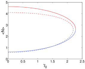
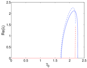
Figure 1: (Color online) Averaged norm (left panel) and real part of the stability eigenvalues (right panel) for a dimer with $\kappa=1$, $E=3$ and $\omega=\gamma_{1}=20$. Solid (dashed) lines represent the values for the averaged (modulated) system, whereas blue (red) corresponds to the S (A) solution. The designation of S (symmetric) or A (anti-symmetric) corresponds to the $\gamma_{0}=0$ Hamiltonian limit of the problem where $\Delta\phi=0$ or $\pi$, respectively.

Figure 2 shows the dynamical evolution of stable and unstable (A and S) solutions. The top panels illustrate a case example of stable oscillations for $\gamma_{0}=1.5$. Notice, however, that this value of the gain/loss parameter is already above the critical one in the absence of modulation, clearly showcasing the extension of the PT-symmetric regime due to the presence of the modulation. Here, the elements of both branches execute stable periodic motion. In the second row, for $\gamma_{0}=2$, the former anti-symmetric oscillation remains stable, but the former symmetric one is in its regime of instability, thus giving rise to a modulated form of growth, whereby the gain site grows indefinitely while the lossy site ultimately approaches a vanishing amplitude. The third row shows the evolution for $\gamma_{0}=2.195$, a value for which both A and S solutions are unstable. At the modified threshold (fourth row) of the PT-symmetry breaking, both branches are sensitive to perturbations and can give rise to growth of one node and decay of the other. This type of behaviour is also generically observed to be relevant for initial data beyond the PT-phase transition threshold, as is shown in the bottom row.

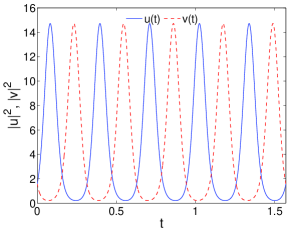
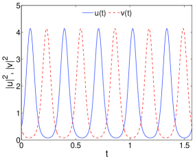
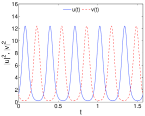
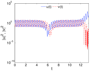
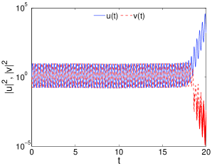
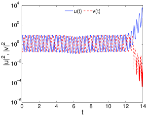
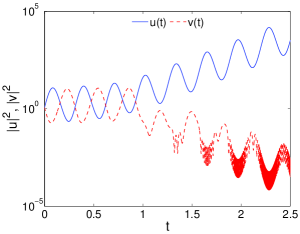
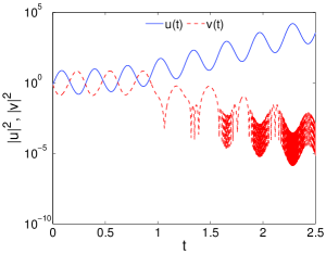
Figure 2: (Color online) Dynamical evolution of former (at $\gamma_{0}=0$) A solutions (left panels) and S solutions (right panels) for the modulated dimer in the case $\kappa=1$, $E=3$, $\gamma_{1}=1$ and $\omega=20$. Top panels correspond to a stable evolution at $\gamma_{0}=1.5$ (which is already beyond the PT-phase transition critical point for $\gamma_{0}$ in the case of $\gamma_{1}=0$); panels of the second row show the stable (unstable) evolution for the A (S) solution at $\gamma_{0}=2$, whereas the third row displays the unstable evolution of solutions at $\gamma_{0}=2.195$. Finally, bottom panels correspond to the evolution at $\gamma_{0}=2.3$ (i.e. past the PT symmetry breaking bifurcation) taking as initial condition the solution at $\gamma_{0}=2.1$.

IV.2 DNLS PT-symmetric trimer model

We now turn to the analysis of the trimer case, where $\kappa^{\prime}=\kappa I_{0}(\gamma_{1})$ and $g^{\prime}=I_{0}(2\gamma_{1})$. In this case, the linear stability eigenvalues of the averaged system are unfortunately not available analytically and are, instead, found by numerical diagonalization. In the numerics, we have chosen the same parameters as in the dimer case except for $E=1$.

In agreement with what has been reported earlier for Schödinger trimers without time-modulation pgk ; kipnew , we have identified three distinct stationary solutions, which will denote hereafter as A, B and C. Solutions A and B exist at $\gamma_{0}=0$ and are characterized, at this limit, in the first case by a phase difference between the sites of $\pi$, so that $u(t)=w(t)\neq v(t)$; in the second case, $v(t)=0$ and there is a phase difference of $\pi$ between the first and third node, i.e. $u(t)=-w(t)$. The third branch of solutions, namely C, exists for $\gamma_{0}\geq\sqrt{2\kappa^{2}I_{0}^{2}(\gamma_{1})-E^{2}}\approx 1.4852$. Interestingly, there is a qualitative difference in the bifurcation diagram (an asymmetric pitchfork, which leads to an isolated branch and a saddle-node bifurcation) between the case examined in Refs. pgk ; kipnew and the one considered herein. In the former, the solutions A and B terminate through a saddle-node and the C solution is the non-bifurcating branch of the broken pitchfork. However, in our present system, it is the B and C solutions which cease to exist at the fold point of $\gamma_{0}=1.5741$, whereas the non-bifurcating branch is now the A one. These results are predicted by the averaged model and corroborated by the numerical analysis of the modulated system and the corresponding numerically exact (up to the prescribed tolerance of $10^{-12}$) time-periodic solutions. Nevertheless, we have checked that for different values of $\kappa^{\prime}$ and $g^{\prime}$, various features of the bifurcation diagram may change. These include the above mentioned possibility of A and B colliding rather than B and C, as well as even the possibility of a fourth (D) branch of solutions emerging in the nonlinear system. The latter case is non-generic, and the bifurcation scheme strongly depends on $\kappa^{\prime}$ and $g^{\prime}$; for instance, at $\kappa^{\prime}=0.1$ and $g^{\prime}=I_{0}(2\gamma_{1})$ the four branches exist at the Hamiltonian limit (with C and D branches corresponding to in phase solutions) and bifurcate branch A with C and B with D through saddle-nodes when $\gamma_{0}$ is increased.

Figure 3 shows both the averaged norm and the stability eigenvalues (imaginary and real parts), together with the predicted values by the averaged equations. Obviously, the prediction of the averaged system is excellent for the B and C solutions, with a small discrepancy arising only for the A solution. We observe that the A solution is stable for small $\gamma_{0}$, becoming unstable through a Hamiltonian Hopf bifurcation footnote2 at $\gamma_{0}=1.5983$ ($1.6261$ in the averaged system). The imaginary part of that quadruplet of eigenvalues becomes zero (i.e., the instability becomes exponential) in the range $\gamma_{0}\in[1.9014,2.1391]$ ($[1.9116,2.1731]$ for the averaged system); the instability becomes again oscillatory above this range. The B solution is oscillatorily unstable for small $\gamma_{0}$, becoming stable via inverse Hopf bifurcation at $\gamma_{0}=1.0216$ ($1.0214$ in the averaged case). The solution becomes exponentially unstable for $\gamma\geq 1.3552$ ($1.3534$, respectively for the effective autonomous equation), finally colliding with the C solution and disappearing in the relevant saddle-node bifurcation at $\gamma_{0}=1.5764$ ($1.5741$ in the averaged system) as explained above. The C solution, which does not exist for $\gamma_{0}<1.4869$ ($1.4852$ in the averaged system), is stable up to $\gamma_{0}=1.5687$ ($1.5667$, respectively for the non-autonomous case), where it experiences an exponential bifurcation. It is clear from the above comparisons that there is an excellent agreement between the predictions of the original system and its effective, averaged description.

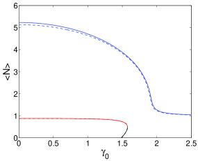
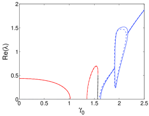
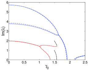
Figure 3: (Color online) Averaged norm (top panel) and stability eigenvalues (bottom panels) for a trimer with $\kappa=1$, $E=1$ and $\omega=\gamma_{1}=20$. Solid (dashed) lines represent the values for the averaged (non-autonomous) system, whereas blue (red) line corresponds to the A (B) solution. The C solution is depicted as a black line.

Figures 4-6 show the dynamical evolution of A, B and C solutions, respectively. In the case of A solutions, we can observe their dynamical stability for sufficiently low values of $\gamma_{0}$ (top left panel). As $\gamma_{0}$ is increased, initially an oscillatory (top right) and subsequently an exponential (bottom left) instability arises. In the dynamical evolutions, the fate of the solutions appears to be similar, with the gain site ultimately growing, while the other two sites are eventually observed to decay in amplitude. Nevertheless, the exponential instability appears to manifest itself faster, in consonance with our eigenvalue findings above. As we progress to higher $\gamma_{0}$, an oscillatory instability arises again, as shown in the bottom right panel but this time with a high growth rate and a rapid destabilization accordingly.

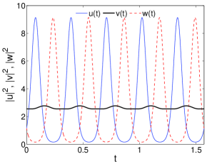
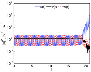
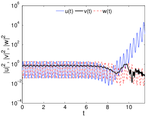
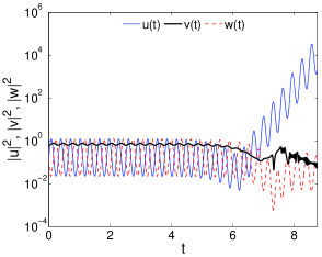
Figure 4: (Color online) Dynamical evolution of A solutions for the modulated trimer in the case $\kappa=1$, $E=1$, $\gamma_{1}=1$ and $\omega=20$. The top left panel corresponds to a stable evolution at $\gamma_{0}=0.5$; the top right panel shows the evolution of an oscillatory unstable solution at $\gamma_{0}=1.8$; the bottom left panel holds for an exponentially unstable solution at $\gamma_{0}=2$; finally, the bottom right panel shows an oscillatorily unstable solution at $\gamma_{0}=2.5$.

The dynamics of the B branch is, arguably, somewhat more complex in Fig. 5. While a stable evolution for $\gamma_{0}=1.2$ is shown in the top left panel, for smaller values of $\gamma_{0}$ (such as $\gamma_{0}=0.5$ of the top right panel), an oscillatory instability is present and appears to lead to indefinite growth of the gain site, while the other two sites decay in amplitude. Perhaps most intriguing is the case of $\gamma_{0}=1.57$ of the bottom left panel of the figure. Here, the dynamics does not appear to diverge, but rather seems to revert to a quasi-periodic motion, yielding a bounded dynamical result. On the other hand, in the bottom right case of $\gamma_{0}=1.7$, past the critical point of the bifurcation with branch C, the dynamics is led to indefinite growth (again with the gain site growing, while the other two are decaying in amplitude).

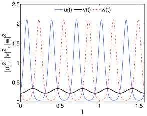
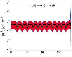
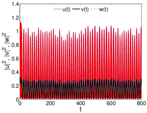
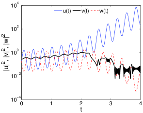
Figure 5: (Color online) Dynamical evolution of B solutions for the modulated trimer in the case $\kappa=1$, $E=1$, $\gamma_{1}=1$ and $\omega=20$. The top left panel corresponds to a stable evolution at $\gamma_{0}=1.2$; the top right panel shows the evolution of an oscillatorily unstable solution at $\gamma_{0}=0.5$; the bottom left panel represents an exponentially unstable solution at $\gamma_{0}=1.57$; finally, the bottom right panel shows the evolution at $\gamma_{0}=1.7$ (i.e. past the collision with branch C) using as initial condition the solution at $\gamma_{0}=1.5$.

Lastly, we consider different dynamical examples from within the narrow interval of existence of branch C in Fig. 6. In the top left panel case of $\gamma_{0}=1.5$, the stable evolution of this branch is depicted. The exponential instability of the branch in the top right panel for $\gamma_{0}=1.57$ appears, similarly to branch B, to lead not to indefinite growth but rather to quasi-periodic oscillation and a bounded dynamical evolution. On the contrary, for values of $\gamma_{0}$ past the saddle-node bifurcation with branch B (but similarly to the dynamics of branch B for such values of $\gamma_{0}$), we observe (cf. bottom left panel) indefinite growth in the dynamics for $\gamma_{0}=1.7$.

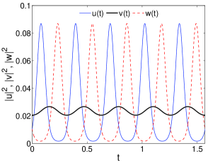
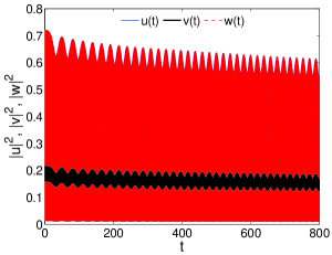
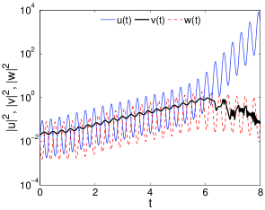
Figure 6: (Color online) Dynamical evolution of C solutions for the modulated trimer in the case $\kappa_{0}=1$, $E=1$ $\gamma_{1}=1$ and $\omega=20$. The top left panel corresponds to a stable evolution at $\gamma_{0}=1.5$; the top right panel shows the evolution of an exponentially unstable solution at $\gamma_{0}=1.57$; the bottom left panel corresponds to the case of $\gamma_{0}=1.7$ (i.e. past the saddle-node bifurcation with branch B) using as initial condition the solution at $\gamma_{0}=1.5$.

V Conclusions and Future Challenges

In the present work, we have explored the potential of PT-symmetric oligomer system (a dimer and a trimer, more concretely, although generalizations to a higher number of sites are directly possible) to have its gain/loss pattern periodically modulated in time. Although this possibility may be somewhat more limited in optical systems, it should in principle be possible in electric circuit settings. As we argued, additionally, this kind of possibility may bear significant advantages including most notably the expansion of the exact PT-symmetric phase region. The latter threshold at the linear level now becomes $\gamma_{0}I_{0}(2\gamma_{1})$ or $\sqrt{2}\gamma_{0}I_{0}(\gamma_{1})$, for the dimer and trimer, respectively, for a modulated gain/loss coefficient with mean value $\gamma_{0}$ and a periodic modulation of amplitude $\gamma_{1}$ and frequency $\omega$. In addition to this expansion, we were able through our averaging procedure to reduce the non-autonomous full problem to an effective time-independent (averaged) one, for which a lot of information (especially so for the dimer case) can be obtained analytically, including the existence and stability of the relevant solutions. The results of the averaged equation approximation were generally found, in the appropriate regime, to be in excellent agreement with those of the full, time-dependent problem and its periodic solutions and their Floquet exponents. This was the case both for the (former) symmetric and asymmetric branches of the dimer and the collision leading to their termination, but also for the branches identified in the trimer, representing an apparent example of an asymmetric pitchfork bifurcation.

One can envision many interesting and relevant extensions of the present work. One such would be to consider the case where the PT-symmetry “management” could be applied to a full lattice or to a chain of dimers, as in the work of dmitriev2 . There, it would be quite relevant to explore the impact of the modulation to the solitary waves and localized solutions of the lattice. Another possibility is to consider generalizations of this “linear” PT-symmetry management towards a nonlinear variant thereof. More specifically, in the spirit of miron ; konorecent ; konorecent2 ; meid , a PT-symmetric gain/loss term could be applied to the nonlinear part of the dimer/trimer or lattice. Then, one can envision a generalization of the notion of nonlinearity management and of the corresponding averaging (see e.g. pelizha ; fkha ), in order to formulate novel effective lattice media as a result of the averaging. Such possibilities are currently under investigation and will be reported in future publications.

- (1) C.M. Bender and S. Boettcher, Phys. Rev. Lett. 80, 5243 (1998); C.M. Bender, S. Boettcher and P.N. Meisinger, J. Math. Phys. 40, 2201 (1999).
- (2) A. Ruschhaupt, F. Delgado, and J.G. Muga, J. Phys. A: Math. Gen. 38 (2005) L171.
- (3) Z.H. Musslimani, K.G. Makris, R. El-Ganainy, and D.N. Christodoulides, Phys. Rev. Lett. 100, 030402 (2008); K.G. Makris, R. El-Ganainy, D.N. Christodoulides, and Z.H. Musslimani, Phys. Rev. A 81, 063807 (2010).
- (4) H. Ramezani, T. Kottos, R. El-Ganainy, and D.N. Christodoulides, Phys. Rev. A 82, 043803 (2010).
- (5) M. Kulishov and B. Kress, Optics Express 20, 29319 (2012).
- (6) C.E. Rüter, K.G. Makris, R. El-Ganainy, D.N. Christodoulides, M. Segev, and D. Kip, Nature Physics 6 (2010) 192.
- (7) A. Guo, G. J. Salamo, D. Duchesne, R. Morandotti, M. Volatier-Ravat, V. Aimez, G. A. Siviloglou and D. N. Christodoulides, Phys. Rev. Lett. 103, 093902 (2009).
- (8) J. Schindler, A. Li, M.C. Zheng, F.M. Ellis, and T. Kottos, Phys. Rev. A 84, 040101 (2011).
- (9) J. Schindler, Z. Lin, J. M. Lee, Hamidreza Ramezani, F. M. Ellis, T. Kottos, J. Phys. A: Math. Theor. 45, 444029 (2012).
- (10) H. Ramezani, T. Kottos, R. El-Ganainy and D.N. Christodoulides, Phys. Rev. A 82, 043803 (2010).
- (11) A.A. Sukhorukov, Z. Xu and Yu.S. Kivshar, Phys. Rev. A 82, 043818 (2010).
- (12) M.C. Zheng, D.N. Christodoulides, R. Fleischmann, and T. Kottos, Phys. Rev. A 82, 010103(R) (2010).
- (13) E.M. Graefe, H.J. Korsch, and A.E. Niederle, Phys. Rev. Lett. 101, 150408 (2008).
- (14) E.M. Graefe, H.J. Korsch, and A.E. Niederle, Phys. Rev. A 82, 013629 (2010).
- (15) Z. Lin, H. Ramezani, T. Eichelkraut, T. Kottos, H. Cao, and D.N. Christodoulides, Phys. Rev. Lett. 106, 213901 (2011).
- (16) K. Li and P. G. Kevrekidis Phys. Rev. E 83, 066608 (2011).
- (17) S.V. Dmitriev, S.V. Suchkov, A.A. Sukhorukov, and Yu.S. Kivshar, Phys. Rev. A 84, 013833 (2011).
- (18) S.V. Suchkov, B.A. Malomed, S.V. Dmitriev and Yu.S. Kivshar, Phys. Rev. E 84, 046609 (2011).
- (19) R. Driben and B. A. Malomed, Opt. Lett. 36, 4323 (2011).
- (20) R. Driben and B. A. Malomed, Europhys. Lett. 96, 51001 (2011).
- (21) F. Kh. Abdullaev, V.V. Konotop, M. Ögren and M. P. Sørensen, Opt. Lett. 36, 4566 (2011).
- (22) N.V. Alexeeva, I.V. Barashenkov, A.A. Sukhorukov, and Yu.S. Kivshar, Phys. Rev. A 85, 063837 (2012).
- (23) A.A. Sukhorukov, S.V. Dmitriev and Yu.S. Kivshar, Opt. Lett. 37, 2148 (2012).
- (24) H. Cartarius and G. Wunner, Phys. Rev. A 86, 013612 (2012); J. Phys. A: Math. Theor. 45, 444008 (2012).
- (25) E.-M. Graefe, J. Phys. A: Math. Theor. 45, 444015 (2012).
- (26) A.S. Rodrigues, K. Li, V. Achilleos, P.G. Kevrekidis, D.J. Frantzeskakis, and C.M. Bender, Rom. Rep. Phys. 65, 5 (2013).
- (27) I. V. Barashenkov, S.V. Suchkov, A.A. Sukhorukov, S.V. Dmitriev, and Yu.S. Kivshar, Phys. Rev. A 86, 053809 (2012).
- (28) I.V. Barashenkov, L. Baker, and N.V. Alexeeva Phys. Rev. A 87, 033819 (2013).
- (29) D.A. Zezyulin and V.V. Konotop, Phys. Rev. Lett. 108, 213906 (2012).
- (30) D. Leykam, V.V. Konotop, and A.S. Desyatnikov, Opt. Lett. 38, 371 (2013).
- (31) K. Li, D. A. Zezyulin, V. V. Konotop, and P. G. Kevrekidis Phys. Rev. A 87, 033812 (2013).
- (32) V. Achilleos, P. G. Kevrekidis, D. J. Frantzeskakis, and R. Carretero-González, Phys. Rev. A 86, 013808 (2012); V. Achilleos, P.G. Kevrekidis, D.J. Frantzeskakis, R. Carretero-González, arXiv:1202.1310.
- (33) Yu.V. Bludov, V.V. Konotop, and B.A. Malomed, Phys. Rev. A 87, 013816 (2013).
- (34) K. Li, P.G. Kevrekidis, B.A. Malomed, and U. Günther, J. Phys. A: Math. Theor. 44, 444021 (2012).
- (35) P.G. Kevrekidis, D.E. Pelinovsky, and D.Y. Tyugin, arXiv:1303.3298, SIAM J. Appl. Dyn. Sys. (in press, 2013); P.G. Kevrekidis, D.E. Pelinovsky, and D.Y. Tyugin, J. Phys. A: Math. Theor. 46, 365201 (2013). arXiv:1307.2973.
- (36) J. Pickton and H. Susanto, arXiv:1307.2788.
- (37) A.E. Miroshnichenko, B.A. Malomed, and Yu.S. Kivshar Phys. Rev. A 84, 012123 (2011).
- (38) F.Kh. Abdullaev, Y.V. Kartashov, V.V. Konotop, and D.A. Zezyulin, Phys. Rev. A 83, 041805 (2011).
- (39) D. A. Zezyulin, Y. V. Kartashov, V. V. Konotop, Europhys. Lett. 96, 64003 (2011).
- (40) M. Duanmu, K. Li, R.L. Horne, P.G. Kevrekidis and N. Whitaker, Phil. Trans. R. Soc. A 371, 20120171 (2013).
- (41) B.A. Malomed, Soliton Management in Periodic Systems (Springer-Verlag, Berlin, 2006).
- (42) S.K. Turitsyn, B.G. Bale, and M.P. Fedoruk, Phys. Rep. 521, 135 (2012).
- (43) Although it is entirely straightforward to envision a modulation of the nonlinear potential too, but this will be deferred as a separate topic for future study.
- (44) K. Li, P.G. Kevrekidis, D.J. Frantzeskakis, C.E. Rüter, D. Kip, arXiv:1306.2255.
- (45) S. Flach and A. V. Gorbach, Phys. Rep. 467, 1 (2008); F. Palmero, L.Q. English, J, Cuevas, R. Carretero-González, and P.G. Kevrekidis, Phys. Rev. E 84, 026605 (2011); T. Cretegny and S. Aubry, Phys. Rev. B 55 R11929 (1997); J. Gómez-Gardeñes, L.M. Floría, M. Peyrard, and A.R. Bishop, Chaos 14, 1130 (2004); T.R.O. Melvin, A.R. Champneys, P.G. Kevrekidis and J. Cuevas, Physica D 237, 551 567 (2008).
- (46) J. Cuevas, P.G. Kevrekidis, A. Saxena and A. Khare, ArXiv: 1307.6047.
- (47) It is interesting to note here that despite the fact that the system is no longer Hamiltonian, the bifurcation arising has all the characteristics of Hamiltonian Hopf including the collision of two eigenvalues and the formation of a quartet. We note that it would be especially interesting to consider the question of the potential existence of an analogous notion to the Krein signature [see, e.g., R. S. MacKay, in Hamiltonian Dynamical Systems, edited by R. S. MacKay and J. Meiss (Hilger, Bristol, 1987), p.137] for these PT-symmetric systems that could predict such potential Hopf bifurcations and quartet formations.
- (48) D.E. Pelinovsky, P.G. Kevrekidis and D.J. Frantzeskakis, Phys. Rev. Lett. 91, 240201 (2003); D.E. Pelinovsky, P.G. Kevrekidis, D.J. Frantzeskakis and V. Zharnitsky, Phys. Rev. E 70, 047604 (2004); V. Zharnitsky and D.E. Pelinovsky, Chaos 15, 037105 (2005); P.G. Kevrekidis, D.E. Pelinovsky and A. Stefanov, J. Phys. A 39, 479 (2006).
- (49) F.Kh. Abdullaev, E.N. Tsoy, and B.A. Malomed, Phys. Rev. A 68,053606 (2013); F.Kh. Abdullaev, P.G. Kevrekidis, and M. Salerno, Phys. Rev. Lett. 105, 113901 (2010).