See pages 1-11 of InversionArXiv.pdf

I Orbital contributions to high-harmonic generation in SO₂

In the main text, we discuss the comparison of the theoretical and experimental contributions to high-harmonic emission using a combination of the photoionization cross-sections weighted by the field ionization calculations. However, in several prior papers [35,40-41], it was observed that the HHG cross spectrum was largely determined solely by the photoionization cross-section, which models the recombination step of HHG. As a result, we examine here a comparison of the theoretical results of photoionization alone to a combination of photoionization and field ionization calculations. The high-harmonic power spectrum at the harmonic energy $\omega$ with the molecular orientation with respect to the laser-field polarization $\hat{u}$ is modeled using the following equation

$$S(\omega,\hat{u})\propto\;\Gamma_{\text{TDSE}}(\vec{u})\;\times\;\sigma(\omega,\hat{u}),$$ (1)

where $S$ is the high-harmonic power spectrum, $\Gamma_{\text{TDSE}}$ is the ionization yield obtained by the solution of the time-dependent Schrödinger equation (TDSE) describing SO₂ exposed to the laser pulse within the one-determinant approximation (see main text) and $\sigma$ is the total one-photon ionization cross-section at a given molecular orientation with respect to the laser polarization.

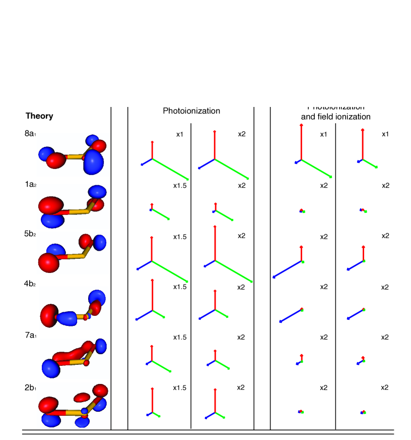
Figure S1: Theoretical and experimental contributions to harmonic emission from all three molecular axes across the first few orbitals of SO₂ for harmonics 19 and 25. First row: the experiment shows a dominance of the b axis for harmonic 19, but shows the b axis as suppressed compared to the a axis contribution for harmonic 25. Middle columns: photoionization cross-sections, which represent the recombination step of HHG. The b axis provides a strong signal for many of the orbitals, but the a axis never shows particular dominance. Right columns: photoionization cross-sections are combined with field-ionization calculations. The a axis is strong and the b axis suppressed for lower-lying orbitals 5b₂, 4b₂, and 7a₁. We thus find that we require the combined calculations of field ionization and photoionization to explain our data.

In Fig. S1 we show some of the highest-lying occupied orbitals of SO₂ (HOMO through HOMO-5) with the orbital ordering obtained from Ref. [34] and their contributions to the harmonics 19 and 25. The middle two columns display the relative contributions from each molecular axis in the experiment (top) and as calculated for one-photon ionization only (bottom). The HHG experiment shows the dominance of the b axis (green) for the 19th harmonic, but a dominant contribution for the a axis in the case of the 25th harmonic (blue). While the HOMO in the one-photon ionization calculation shows a strong b axis contribution for both the 19th and the 25th harmonics, none of the HOMO or lower-lying orbitals show a particularly strong contribution from the a axis. The photoionization calculation on its own is thus insufficient to explain the experiment.

However, looking at the combined photoionization and TDSE strong-field ionization results, we see that the lower-lying orbitals do show a dominance of the a axis for both harmonic energies. This points to strong-field ionization (often in a simplified way referred to as tunneling ionization) as being crucial to fully explain the inversion of signal enhancement present in our experimental data. We thus find that for some cases, a calculation of the photoionization cross-section alone is insufficient to explain the data and that care should be taken when employing such a calculation on its own.

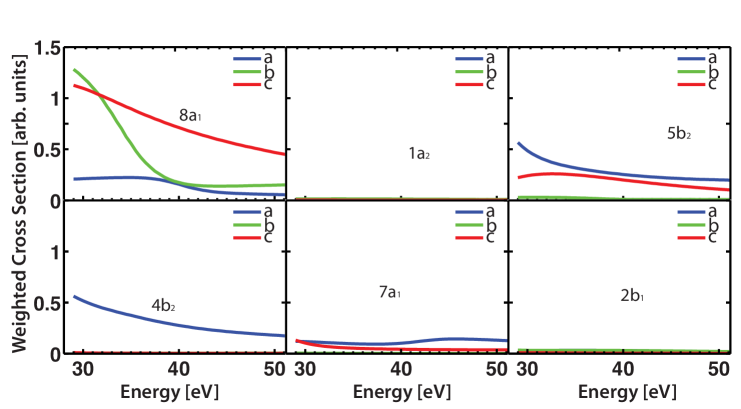
Figure S2: One-photon ionization cross-sections weighted by the strong-field ionization yield for the highest-lying occupied orbitals. The lower-lying orbitals 5b₂, 4b₂, and 7b₂ show a dominance of the a axis throughout the whole energy range. The lower-lying orbitals contribute more directly to the signal of higher order harmonics.

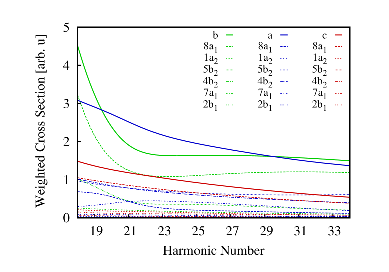
Figure S3: Sum of the contribution of the first few orbitals for the main directions of the SO₂ one-photon ionization cross-sections weighted by the strong-field ionization yield at an intensity of 2.6 $\times$ 10¹⁴ W/cm². The non-solid curves indicate the contribution of each orbital to incoherent sum.

For clarity, in the main text we limited our discussion to harmonics 19 and 25. However, we examined all harmonics to ensure that our analysis was consistent. In Fig. S2 we show the combined photoionization and field-ionization results as a function of energy over the whole energy range of the harmonics 19 to 33. Figure S2 shows that the dominance of the a axis that we observe in the lower-lying orbitals 5b₂, 4b₂, and 7a₁ is consistent throughout the energy range. Furthermore, it shows that the HOMO signal switches from being most pronounced when the laser field is aligned parallel to the b axis to the situation when it is aligned along the c axis. Our analysis of the data shows a switch from the b axis at lower harmonics to the a axis at higher harmonics as shown in Fig. 3 of the main text. Thus, the explanation that the 19th harmonic receives a dominant signal from the 8a₁ orbital while the higher harmonics receive dominant signals from the 5b₂, 4b₂, and 7a₁ is consistent with our analysis of all harmonics.

Fig. S3 shows the total incoherent sum of the contributions of the different orbitals under study. Here one can see again the dominance of the b axis for the harmonic 19 and the dominance of the a axis for harmonic 25 due to a crossing in the curve.

II Effects of Laser Intensity on Strong-Field Ionization

Since the experimental laser intensity is a parameter that is not precisely known, we also consider the effects of laser intensity on the ion yields obtained when solving the TDSE.

Figure S4 (similar to Fig. S3, but for better clarity without the orbital contributions) shows the strong-field weighted cross-sections for different peak intensities of the laser. Evidently, the crossing of the blue and green curves (a and b axes ) moves with intensity, but it exists for quite some intensity range (although it disappears for lower intensities). Interestingly, one sees also that for higher intensities the red curve (c axis) increases and shows a crossing with the green one (b axis), as in the experiment. However, we do not see a sharp decrease of the red curves for low HHG numbers, as seen in the experiment for high harmonic 19. Furthermore, one sees also that the blue and the green curves start to approach each other for higher HHG numbers, a similar trend as in the experiment.

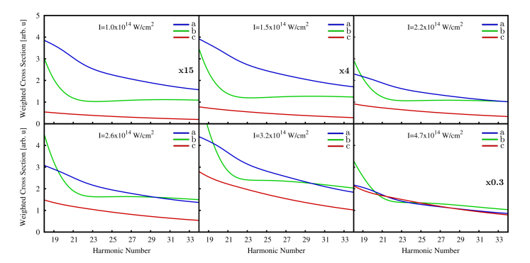
Figure S4: SO₂ one-photon ionization cross-sections sum weighted by the strong-field ionization yield at different intensities using the theoretical ionization potentials.

Figure S5 shows results for the same parameters as in Fig. S4, but now obtaining the energy axis using experimental ionization thresholds in the calculation of the one-photon ionization cross-sections. The main finding of the first graph does not change, although the crossing shifts slightly.

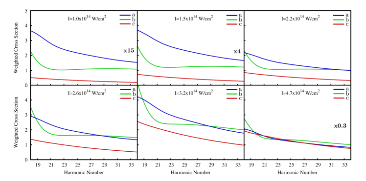
Figure S5: Similar to Fig. S4, but using the experimental ionization potentials

We see the crossing due to lower lying orbitals confirmed, and the crossing position lies very close to the experimental one. Furthermore, the crossing and its position is intensity dependent, but it changes rather systematically with intensity and, again, it occurs around the experimental intensity. In fact, the crossing of the green and the red curves seen in the experiment is somehow consistent with the calculation, although the intensities would be higher than the experimentally specified one.

III Comparison of the Photoionization Cross Sections

To ensure that the recombination cross-sections were accurately calculated, we calculated photoionization cross-sections using two different methods, as mentioned in the main text. A comparison of the two methods is shown in Fig. S6. Fig. S6a shows results obtained with the first approach that is based on the complex Kohn variational method. These results were used in creating the combined probabilities in Fig. 4 of the main text. Fig. S6b shows the results obtained with the second approach. Although there are some differences between the calculations, they do not influence the overall result when comparing to the data or when combined with strong-field ionization calculations.

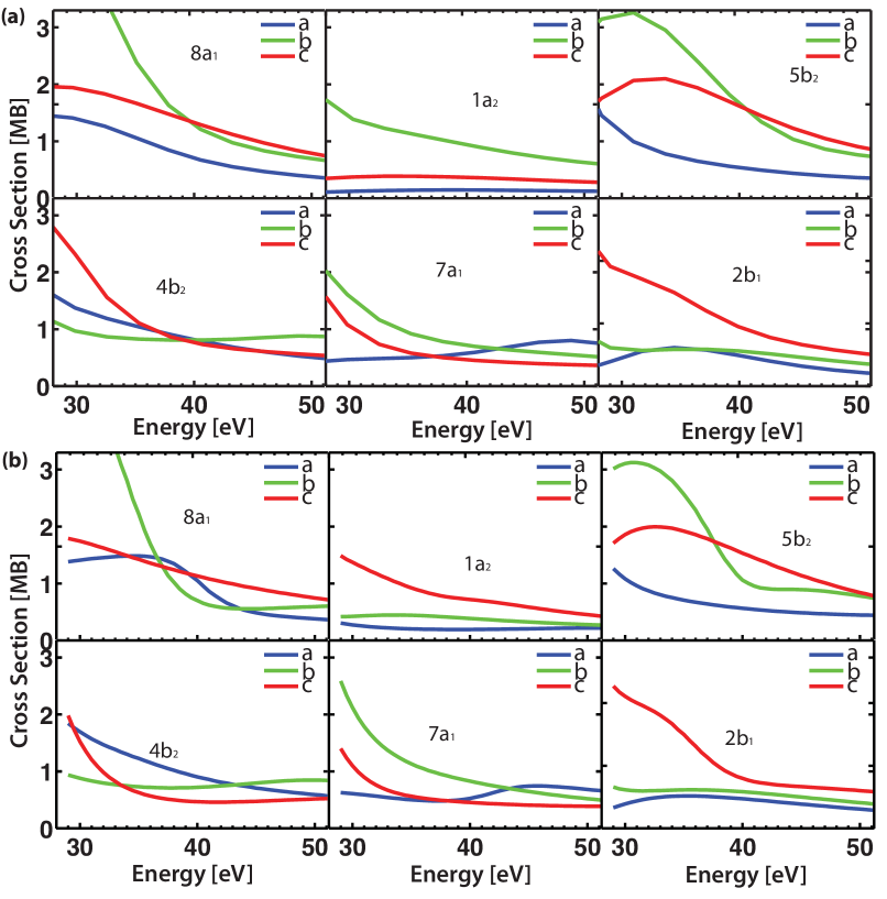
Figure S6: A comparison of photoionization cross-section calculations with two different methods. a) Results based on the complex Kohn variational method. These results were used to create the combined results in Fig. 4 of the main text. b) Results obtained using the density-functional theory approach. The minor differences do not influence the overall result when comparing to data or when combined with field-ionization calculations.