On the causal interpretation of acyclic mixed graphs under multivariate normality

Abstract.

In multivariate statistics, acyclic mixed graphs with directed and bidirected edges are widely used for compact representation of dependence structures that can arise in the presence of hidden (i.e., latent or unobserved) variables. Indeed, under multivariate normality, every mixed graph corresponds to a set of covariance matrices that contains as a full-dimensional subset the covariance matrices associated with a causally interpretable acyclic digraph. This digraph generally has some of its nodes corresponding to hidden variables. We seek to clarify for which mixed graphs there exists an acyclic digraph whose hidden variable model coincides with the mixed graph model. Restricting to the tractable setting of chain graphs and multivariate normality, we show that decomposability of the bidirected part of the chain graph is necessary and sufficient for equality between the mixed graph model and some hidden variable model given by an acyclic digraph.

1. Introduction

Acyclic digraphs are standard representations of causally interpretable statistical models in which the involved random variables are noisy functions of each other, with all noise terms being independent. In generalization, acyclic mixed graphs with directed and bidirected edges are widely used for compact representation of causal structure when important variables are hidden (that is, unobserved) [Pea09, SGS00, Kos02, RS02, Wer11]. Such mixed graphs are also known as path diagrams in the field of structural equation modeling [Bol89, Kos99]. The graphs provide, in particular, a framework for statistical model selection in the presence of hidden variables [CMKR12, SGS00, SG09].

Under joint multivariate normality, it is well-known that for every acyclic mixed graph there exists an acyclic digraph, generally with additional vertices, such that the statistical model associated with the digraph is a full-dimensional subset of the model determined by the mixed graph. Here, nodes that appear in the digraph but not in the mixed graph are treated as hidden variables and marginalized over. In this paper we ask which mixed graphs induce a statistical model that is not only a superset but equal to a hidden variable model given by some acyclic digraph. We focus on the particularly tractable class of chain graphs, that is, mixed graphs without semi-directed cycles. Our main result characterizes the chain graphs for which there exists an acyclic digraph with hidden variable model equal to the chain graph model. We begin by formally introducing the concerned graphical models and stating the precise form of the problem and main result.

Let $\mathcal{D}=(V,E)$ be an acyclic digraph with finite vertex set $V$ and edge set $E\subseteq V\times V$. We denote possible edges $(u,v)$ by $u\to v$. Let $\mathbb{R}^{E}$ be the set of matrices $\Lambda=(\lambda_{uv})\in\mathbb{R}^{V\times V}$ that are supported on $E$, that is, $\lambda_{uv}=0$ if $u\to v\not\in E$ or $u=v$. For any $\Lambda\in\mathbb{R}^{E}$, the matrix $I-\Lambda$ is invertible because $\det(I-\Lambda)=1$. Throughout, $I$ denotes the identity matrix with size determined by the context.

Definition 1.1.

The Gaussian graphical model $\mathbf{N}(\mathcal{D})$ is the family of all multivariate normal distributions $\mathcal{N}(\mu,\Sigma)$ on $\mathbb{R}^{V}$ that have covariance matrix

(1.1) $$\Sigma=(I-\Lambda)^{-T}\Omega(I-\Lambda)^{-1}$$

with $\Lambda\in\mathbb{R}^{E}$ and $\Omega\in\mathbb{R}^{V\times V}$ diagonal with positive diagonal entries.

The motivation for consideration of the model $\mathbf{N}(\mathcal{D})$ becomes clearer through the following construction. Let $\epsilon=(\epsilon_{v})_{v\in V}$ be a multivariate normal random vector with covariance matrix $\Omega=(\omega_{uv})$, and let ${\rm pa}(v)=\{u\,:\,u\to v\in E\}$ be the set of parents of vertex $v$. Define the random vector $X=(X_{v})_{v\in V}$ to be the solution of the linear equation system

(1.2) $$X_{v}=\lambda_{0v}+\sum_{u\in{\rm pa}(v)}\lambda_{uv}X_{u}+\epsilon_{v},\qquad v\in V.$$

Then $X$ is multivariate normal with covariance matrix as in (1.1), where $\Lambda\in\mathbb{R}^{E}$ contains the coefficients in the equations in (1.2), which are also known as structural equations [Bol89]. The distributions in $\mathbf{N}(\mathcal{D})$ thus arise when the considered random variables are related via noisy functional, or in other words, causal relationships. We refer the reader to [Lau96] or [DSS09, Chap. 3] for general background on graphical models, and to [Pea09] and [SGS00] for details on causal interpretation.

While noisy functional relationships are often natural for modelling dependences among observed random variables $X_{v}$, $v\in V$, many applications face the problem that additional variables may appear in the functions. The relevant acylic digraph $\mathcal{D}=(U,E)$ has then a larger vertex set $U\supseteq V$ and edge set $E\subseteq U\times U$. The nodes in $U\setminus V$ correspond to so-called hidden (or latent) variables that remain unobserved. The pair $(\mathcal{D},V)$ determines a hidden variable model $\mathbf{N}_{V}(\mathcal{D})$ comprising the normal distributions on $\mathbb{R}^{V}$ that arise as $V$-marginal of a distribution in $\mathbf{N}(\mathcal{D})$.

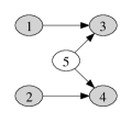
(a)           (b)

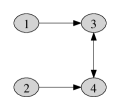
Figure 1.1. (a) An acyclic digraph $\mathcal{D}$. (b) Mixed graph for the marginal distribution of $(X_{1},\dots,X_{4})$.

Example 1.1.

Consider the acyclic digraph $\mathcal{D}=(U,E)$ from Figure 1.1(a) with vertex set $U=\{1,\dots,5\}$. If we only observe the random variables indexed by the nodes in $V=\{1,\dots,4\}$, then the covariance matrices of the normal distributions in $\mathbf{N}_{V}(\mathcal{D})$ have the form

(1.3) $$\begin{pmatrix}\omega_{11}&0&\lambda_{13}\omega_{11}&0\\ 0&\omega_{22}&0&\lambda_{24}\omega_{22}\\ \lambda_{13}\omega_{11}&0&\lambda_{13}^{2}\omega_{11}+\omega_{33}+\lambda_{53}^{2}\omega_{55}&\lambda_{53}\lambda_{54}\omega_{55}\\ 0&\lambda_{24}\omega_{22}&\lambda_{53}\lambda_{54}\omega_{55}&\lambda_{24}^{2}\omega_{22}+\omega_{44}+\lambda_{54}^{2}\omega_{55}\end{pmatrix},$$

where $\omega_{11},\dots,\omega_{55}>0$ are the variances of the error terms in (1.2). The four edges in $\mathcal{D}$ correspond to the coefficients $\lambda_{13},\lambda_{24},\lambda_{53},\lambda_{54}\in\mathbb{R}$.

Many acylic digraphs give the same hidden variable model over a particular set of observed nodes $V$. For instance, if we add a sixth node and the edges $3\leftarrow 6\to 4$ to the graph $\mathcal{D}$ from Figure 1.1(a), then the resulting graph $\mathcal{D}^{\prime}$ satisfies $\mathbf{N}_{V}(\mathcal{D}^{\prime})=\mathbf{N}_{V}(\mathcal{D})$ for $V=\{1,\dots,4\}$. Due to this fact, it is often useful to represent hidden variable models by mixed graphs whose nodes correspond only to observed variables but whose edge set may contain a second type of edge.

Mixed graphs are triples $\mathcal{G}=(V,D,B)$ that consist of a finite vertex set $V$ and two sets of edges $D,B\subseteq V\times V$. The set $D$ contains directed edges, denoted again by $u\to v$. The pairs in $B$ are bidirected edges, which we write as $v\leftrightarrow w$. The bidirected edges do not have an orientiation, that is, $v\leftrightarrow w\in B$ if and only if $w\leftrightarrow v\in B$. We tacitly assume absence of self-loops, that is, $(v,v)\not\in D\cup B$ for all $v\in V$. A mixed graph is acyclic if its directed part $(V,D)$ is an acyclic digraph.

For an acyclic mixed graph $\mathcal{G}=(V,D,B)$, let $\mathbb{R}^{D}$ be the set of $V\times V$-matrices $\Lambda=(\lambda_{uv})$ supported on $D$. Similarly, let $\mathit{PD}(B)$ be the cone of positive definite $V\times V$-matrices $\Omega=(\omega_{uv})$ supported on $B$, with the distinction that the diagonal entries are not constrained to be zero. Mixed graph models are defined in analogy to the models given by digraphs, the sole difference being the fact that the error terms in (1.2) need no longer be mutually independent.

Definition 1.2.

The Gaussian mixed graph model $\mathbf{N}(\mathcal{G})$ is the family of all multivariate normal distributions $\mathcal{N}(\mu,\Sigma)$ on $\mathbb{R}^{V}$ that have covariance matrix

$$\Sigma=(I-\Lambda)^{-T}\Omega(I-\Lambda)^{-1}$$

with $\Lambda\in\mathbb{R}^{D}$ and $\Omega\in\mathit{PD}(B)$.

A mixed graph model does not have an a priori causal interpretation because no causal mechanism is specified for generating the dependences that may exist among the error terms $\epsilon_{v}$, $v\in V$. However, as we suggested above, such a causal interpretation can be given via hidden variables.

Example 1.2.

The distributions in the model $\mathbf{N}(\mathcal{G})$ defined by the mixed graph $\mathcal{G}$ in Figure 1.1(b) have covariance matrix

(1.4) $$\begin{pmatrix}\omega_{11}&0&\lambda_{13}\omega_{11}&0\\ 0&\omega_{22}&0&\lambda_{24}\omega_{22}\\ \lambda_{13}\omega_{11}&0&\omega_{33}+\lambda_{13}^{2}\omega_{11}&\omega_{34}\\ 0&\lambda_{24}\omega_{22}&\omega_{34}&\omega_{44}+\lambda_{24}^{2}\omega_{22}\end{pmatrix},$$

where $\lambda_{13},\lambda_{24}\in\mathbb{R}$ and the five parameters $\omega_{ij}$ form a positive definite $4\times 4$ matrix with all off-diagonal entries zero except for $\omega_{34}$. It is not difficult to show that the matrix in (1.4) can always be written as in (1.3), and vice versa. Hence, $\mathbf{N}(\mathcal{G})=\mathbf{N}_{V}(\mathcal{D})$ for the graph $\mathcal{D}$ from Figure 1.1(a) and the nodes in $V=\{1,\dots,4\}$.

The two graphs in Figure 1.1 are related through a well-known general construction. For each bidirected edge $u\leftrightarrow v$ in a mixed graph $\mathcal{G}$ introduce a new node $h_{\{u,v\}}$. Then replace the edge $u\leftrightarrow v$ by the two edges $u\leftarrow h_{\{u,v\}}\to v$. The resulting digraph $\mathcal{D}$ has been called the bidirected subdivision in [STD10] and the canonical DAG (short for acyclic digraph) in [RS02]; it also underlies the semi-Markovian models of [Pea09]. As used in [STD10], the construction yields for every mixed graph $\mathcal{G}=(V,D,B)$ a digraph $\mathcal{D}=(U,E)$ with $V\subseteq U$ such that $\mathbf{N}_{V}(\mathcal{D})$ is a full-dimensional subset of $\mathbf{N}(\mathcal{G})$; to make this a formal statement, identify each model with the set of covariance matrices of its probability distributions. Hence, every mixed graph model can be regarded as a “closure” of the causal (hidden variable) model defined by its canonical digraph.

While the mixed graph from Figure 1.1(b) and its canonical digraph in Figure 1.1(a) define exactly the same model for the random vector $(X_{1},\dots,X_{4})$, it is known from the examples in [RS02] and [DY10] that the canonical digraph sometimes only defines a proper submodel. It remains an open problem to characterize the acyclic mixed graphs that have the following strict causal interpretation.

Definition 1.3.

An acyclic mixed graph $\mathcal{G}=(V,D,B)$ is strictly Gaussian causal if there exists an acyclic digraph $\mathcal{D}=(U,E)$ on $U\supseteq V$ with $\mathbf{N}_{V}(\mathcal{D})=\mathbf{N}(\mathcal{G})$.

We would like to emphasize that the acyclic digraphs in Definition 1.3 are entirely arbitrary. Hence, unlike canonical DAGs, they may feature hidden nodes in $U\setminus V$ with more than two children.

The following result is known about graphs without directed edges. Recall that the bidirected part $(V,B)$ is decomposable (or chordal or triangulated) if it has no induced cycles of length more than three.

Theorem 1.1 ([DY10]).

If $\mathcal{G}=(V,\emptyset,B)$ is a mixed graph without directed edges, then it is strictly Gaussian causal if $(V,B)$ is decomposable.

In this paper we first clarify that the hidden variable construction underlying the proof of Theorem 1.1 also yields that this condition is sufficient in general.

Theorem 1.2.

If an acyclic mixed graph $\mathcal{G}=(V,D,B)$ has a decomposable bidirected part $(V,B)$, then $\mathcal{G}$ is strictly Gaussian causal.

We remark that it is meaningful to extend Definition 1.2 to non-acyclic mixed graphs, restricting the matrices $\Lambda\in\mathbb{R}^{D}$ to have $I-\Lambda$ invertible. Then Theorem 1.2 would still apply if Definition 1.3 were changed to allow for cyclic digraphs.

In general, the decomposability of the bidirected part is not necessary for strict Gaussian causality of an acyclic mixed graph; see Example 2.1. However, it is necessary when $\mathcal{G}=(V,D,B)$ is a chain graph, which refers to a mixed graph without semi-directed cycles. An $n$-cycle $(v_{1},v_{2}),(v_{2},v_{3}),\dots,(v_{n},v_{1})\in D\cup B$ is semi-directed if at least one of its edges is in $D$; any directed edge $(v_{i},v_{i+1})\in D$ on this cycle is traversed in the same orientation $v_{i}\to v_{i+1}$. We remark that the statistical interpretation of chain graphs in [Lau96] differs from the one in this paper; see also [Drt09, WC04].

Theorem 1.3.

Suppose the mixed graph $\mathcal{G}=(V,D,B)$ is a chain graph. Then $\mathcal{G}$ is strictly Gaussian causal if and only if the bidirected part $(V,B)$ is decomposable.

A chain graph is simple (that is, $D\cap B=\emptyset$), and the connected components of its bidirected part are also known as chain components. Each chain component induces a subgraph that is bidirected, that is, does not contain any edge in $D$. Moreover, for a chain graph, the model $\mathbf{N}(\mathcal{G})$ can also be defined by conditional independence constraints among the observed random variables. We use this fact in our proof of necessity in Theorem 1.3, which also involves a sign-change trick from [DY10] and results on subdeterminants of the covariance matrix in (1.1) due to [STD10]. We remark that proving a mixed graph not to be strictly Gaussian causal requires arguments about an infinite set of acyclic digraphs. This is in contrast to many other Markov equivalence problems, where all considered graphs have the same vertex set [PW94, DR08, ZZL05, ARS09, WS12].

The remainder of the paper is organized as follows. In Section 2, we prove Theorem 1.2. Section 3 reviews background needed for the proof of Theorem 1.3, which is the topic of Section 4. We conclude with a discussion of the treated problem in Section 5.

2. Mixed graphs with decomposable bidirected part

In this section we prove Theorem 1.2 according to which an acyclic mixed graph $\mathcal{G}=(V,D,B)$ with decomposable bidirected part $(V,B)$ is strictly Gaussian causal. Let $\mathcal{C}$ be the set of all cliques of the part $(V,B)$, where a set $C\subset V$ is a clique if $u\leftrightarrow v\in B$ for any two distinct nodes $u,v\in C$. Let $\mathcal{C}_{2}\subset\mathcal{C}$ be the set of cliques that have two or more elements. We will use the following construction.

Definition 2.1.

We define the clique digraph of a mixed graph $\mathcal{G}=(V,D,B)$ to be the acyclic digraph $\mathcal{D(G)}=(U,E)$ with $U=V\cup\mathcal{C}_{2}$ and

$$E=D\cup\{h\to v\,:\,h\in\mathcal{C}_{2},\,v\in h\}.$$

The clique digraph contains a new node for every non-singleton clique in $(V,B)$, and links each new node to all nodes appearing in the concerned clique. Figure 2.1 shows an example. If $(V,B)$ contains only cliques of size at most two, then the clique digraph is equal to the aforementioned bidirected subdivision/canonical DAG.

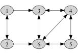
(a)       (b)

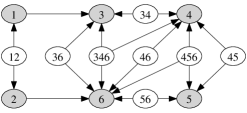
Figure 2.1. (a) A chain graph $\mathcal{G}$ with decomposable bidirected part. (b) The clique digraph $\mathcal{D(G)}$; unshaded nodes correspond to cliques and represent the hidden variables.

Proof of Theorem 1.2.

Let $\mathcal{D(G)}=(U,E)$ be the clique digraph of the acyclic mixed graph $\mathcal{G}=(V,D,B)$, with $U=V\cup\mathcal{C}_{2}$. Let $\Gamma$ be a $U\times U$ matrix in $\mathbb{R}^{E}$, and let $\Delta$ be a diagonal $U\times U$ matrix with positive diagonal entries. Based on the partitioning $U=V\cup\mathcal{C}_{2}$, we have

$$\Gamma =\begin{pmatrix}\Gamma_{11}&0\\ \Gamma_{21}&0\end{pmatrix}, \Delta =\begin{pmatrix}\Delta_{11}&0\\ 0&\Delta_{22}\end{pmatrix},$$

where $\Gamma_{11},\Delta_{11}$ are in $\mathbb{R}^{V\times V}$ and $\Delta_{22}$ is in $\mathbb{R}^{\mathcal{C}_{2}\times\mathcal{C}_{2}}$. Due to the triangular form of $I-\Gamma$, we have

$$(I-\Gamma)^{-1}=\begin{pmatrix}(I-\Gamma_{11})^{-1}&0\\ \Gamma_{21}(I-\Gamma_{11})^{-1}&I\end{pmatrix}.$$

The covariance matrices for the distributions in $\mathbf{N}_{V}(\mathcal{D(G)})$ are thus of the form

$$\Sigma =\left[(I-\Gamma)^{-T}\Delta(I-\Gamma)^{-1}\right]_{V\times V}$$

(2.1) $$=(I-\Gamma_{11})^{-T}\left[\begin{pmatrix}I&0\\ -\Gamma_{21}&I\end{pmatrix}^{-T}\Delta\begin{pmatrix}I&0\\ -\Gamma_{21}&I\end{pmatrix}^{-1}\right]_{V\times V}(I-\Gamma_{11})^{-1}$$

$$=(I-\Gamma_{11})^{-T}(\Delta_{11}+\Gamma_{21}^{T}\Delta_{22}\Gamma_{21})(I-\Gamma_{11})^{-1}.$$

Since two columns of $\Gamma_{21}$ have disjoint support unless the corresponding two nodes are in a clique in $\mathcal{C}_{2}$, or equivalently, unless the two nodes are adjacent in $\mathcal{G}$, the matrix

(2.2) $$\Delta_{11}+\Gamma_{21}^{T}\Delta_{22}\Gamma_{21}$$

is a positive definite matrix in $\mathit{PD}(B)$. Hence, $\mathbf{N}_{V}(\mathcal{D(G)})\subseteq\mathbf{N}(\mathcal{G})$. However, more is true. According to (2.1), the matrix in (2.2) is a covariance matrix associated with the clique digraph of the mixed graph $(V,\emptyset,B)$. The proof of Theorem 1.1 in [DY10] shows that, for $(V,B)$ decomposable, any matrix in $\mathit{PD}(B)$ can be written in the form (2.2). We conclude that $\mathbf{N}_{V}(\mathcal{D(G)})=\mathbf{N}(\mathcal{G})$. ∎

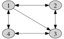
(a)           (b)

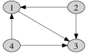
Figure 2.2. (a) An acyclic mixed graph that has non-decomposable bidirected part but is strictly Gaussian causal. (b) An acyclic digraph determining the same model.

The next example shows that decomposability of the bidirected part of an acyclic mixed graph is not necessary for strict Gaussian causality.

Example 2.1.

Let $\mathcal{G}$ be the mixed graph depicted in Figure 2.2(a). The bidirected part of this graph is a four-cycle, so not decomposable. However, $\mathcal{G}$ is strictly Gaussian causal because $\mathbf{N}(\mathcal{G})=\mathbf{N}(\mathcal{D})$ for the acyclic digraph $\mathcal{D}$ from Figure 2.2(b).

The two graphs $\mathcal{G}$ and $\mathcal{D}$ in Figure 2.2 have the same vertex set, and the fact that $\mathbf{N}(\mathcal{G})=\mathbf{N}(\mathcal{D})$ is an instance of Markov equivalence of two mixed graphs that are ancestral in the sense of [RS02]. More generally, for ancestral graphs, the sufficient condition from Theorem 1.2 could be strengthened by first applying results on the characterization of Markov equivalence of ancestral graph [ARS09, ZZL05] to convert a given ancestral mixed graph $\mathcal{G}$ to another ancestral mixed graph $\mathcal{G^{\prime}}$ with $\mathbf{N}(\mathcal{G})=\mathbf{N}(\mathcal{G^{\prime}})$ with fewer bidirected edges; this is in the spirit of [DR08]. If the bidirected part of $\mathcal{G^{\prime}}$ is decomposable, then Theorem 1.2 can be applied.

3. Treks, systems of treks and d-connecting walks

For a proof of Theorem 1.3, which is the topic of Section 4, we need to be able to make arguments about the structure of an acyclic digraph $\mathcal{D}$ that determines a hidden variable model equal to a given chain graph model $\mathbf{N}(\mathcal{G})$. In preparation, we collect in this section known results about the combinatorial structure of the covariance matrices of distributions in $\mathbf{N}(\mathcal{D})$.

Let $\mathcal{D}=(U,E)$ be any acyclic digraph. A walk $\pi$ from source node $u$ to target node $v$ in $\mathcal{D}$ is a sequence of edges in $E$ connecting the consecutive nodes in a sequence of nodes starting at $u$ and ending at $v$. If $\pi$ visits all of its nodes only once, then it is a path. If all edges are traversed according to their orientation, then the walk $\pi$ is a directed path from $u$ to $v$; it is a path because visiting a node twice would result in a directed cycle. A collider on a walk $\pi$ from $u$ to $v$ is an interior node $w$ (i.e., $w\notin\{u,v\}$) such that the two edges of $\pi$ that are incident to $w$ have their “arrowheads collide” as $w^{\prime}\to w\leftarrow w^{\prime\prime}$.

A trek $\tau$ from $u$ to $v$ is a walk without colliders and takes the form:

(3.1) $$v^{\text{L}}_{l}\leftarrow v^{\text{L}}_{l-1}\leftarrow\dots\leftarrow v^{\text{L}}_{1}\leftarrow v^{\text{T}}\to v^{\text{R}}_{1}\to\dots\to v^{\text{R}}_{r-1}\to v^{\text{R}}_{r},$$

where the endpoints are $v^{\text{L}}_{l}=u$, $v^{\text{R}}_{r}=v$. We say that $\mathrm{Left}\left({\tau}\right)=\{v^{\text{T}},v^{\text{L}}_{1},\dots,v^{\text{L}}_{l}\}$ is the left-hand side of $\tau$, and similarly, $\mathrm{Right}\left({\tau}\right)=\{v^{\text{T}},v^{\text{R}}_{1},\dots,v^{\text{R}}_{r}\}$ is the right-hand side. The top node $v^{\text{T}}=\mathrm{Top}\left({\tau}\right)$ is contained in both sides of the trek. Though a trek in an acyclic digraph has no repetition of nodes on either the right- or left-hand side, it may contain the same node once on its left-hand side and once again on its right-hand side and thus not be a path. Every directed walk is a trek with $|\mathrm{Left}\left({\tau}\right)|=1$ or $|\mathrm{Right}\left({\tau}\right)|=1$ depending on the orientation of the edges. A trek is allowed to be trivial, that is, for every node $v\in U$, there is a trek $\tau$ from $v$ to $v$ that contains no edges and has $\mathrm{Left}\left({\tau}\right)=\mathrm{Right}\left({\tau}\right)=\{v\}$ and $\mathrm{Top}\left({\tau}\right)=v$.

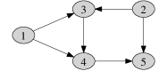
Figure 3.1. An acyclic digraph.

Example 3.1.

In the graph shown in Figure 3.1, the path $\pi_{1}:3\leftarrow 1\to 4\to 5$ is a trek with $\mathrm{Left}\left({\pi_{1}}\right)=\{1,3\}$, $\mathrm{Right}\left({\pi_{1}}\right)=\{1,4,5\}$, and $\mathrm{Top}\left({\pi_{1}}\right)=1$. Similarly, the walk $\pi_{2}:4\leftarrow 3\leftarrow 1\to 3\to 4\to 5$ is a trek with $\mathrm{Left}\left({\pi_{2}}\right)=\{1,3,4\}$, $\mathrm{Right}\left({\pi_{2}}\right)=\{1,3,4,5\}$, and $\mathrm{Top}\left({\pi_{2}}\right)=1$. The walk $\pi_{3}:3\rightarrow 4\leftarrow 1\to 3$ is not a trek due to the collider at node 4.

Let $\Lambda=(\lambda_{uv})\in\mathbb{R}^{E}$, and let $\Omega=(\omega_{vv})$ be a diagonal $U\times U$ matrix with positive diagonal entries. If a covariance matrix $\Sigma=(\sigma_{uv})$ satisfies $\Sigma=(I-\Lambda)^{-T}\Omega(I-\Lambda)^{-1}$ as in (1.1), then the matrix $\Lambda\in\mathbb{R}^{E}$ and the diagonal matrix $\Omega$ in this representation are unique. Indeed, if $u\to v\in E$, then $\lambda_{uv}$ corresponds to entry $u$ in the vector

(3.2) $$\Sigma_{v,{\rm pa}(v)}\left(\Sigma_{{\rm pa}(v),{\rm pa}(v)}\right)^{-1}$$

and $\omega_{vv}$ is a Schur complement, namely,

(3.3) $$\omega_{vv}=\sigma_{vv}-\Sigma_{v,{\rm pa}(v)}\left(\Sigma_{{\rm pa}(v),{\rm pa}(v)}\right)^{-1}\Sigma_{{\rm pa}(v),v}.$$

For a general discussion of this uniqueness see [DFS11].

For a trek $\tau$ in $\mathcal{D}$ with $\mathrm{Top}\left({\tau}\right)=t$, define the trek monomial

(3.4) $$\sigma(\tau)=\omega_{tt}\prod_{x\to y\in\tau}\lambda_{xy}.$$

The unique representation implies that the value of the trek monomial $\sigma(\tau)$ is determined by $\Sigma$ via (3.2) and (3.3). The following rule expresses the entries of a covariance matrix as sums of trek monomials [SGS00, Wri21, Wri34].

Lemma 3.1 (Trek rule).

The covariance matrix $\Sigma=(\sigma_{uv})$ of a distribution from $\mathbf{N}(\mathcal{D})$ has the entries

(3.5) $$\sigma_{uv}=\sum_{\tau\in\mathcal{T}(u,v)}\sigma(\tau),$$

where $\mathcal{T}(u,v)$ is the set of all treks from $u$ to $v$, which is finite.

In the treatment of chain graphs we will have information about subdeterminants rather than entries of the covariance matrix. This will require us to consider sets of treks $\Pi=\{\tau_{1},\dots,\tau_{n}\}$. Let $x_{i}$ and $y_{i}$ be the source and the target of each trek $\tau_{i}$, respectively. If all sources and all targets are distinct, then we call $\Pi$ a system of treks from $X=\{x_{1},\dots,x_{n}\}$ to $Y=\{y_{1},\dots,y_{n}\}$, denoted as $\Pi:X\rightrightarrows Y$. This allows $X\cap Y\not=\emptyset$. If

$$\mathrm{Left}\left({\tau_{i}}\right)\cap\mathrm{Left}\left({\tau_{j}}\right)=\emptyset=\mathrm{Right}\left({\tau_{i}}\right)\cap\mathrm{Right}\left({\tau_{j}}\right)$$

for all $i\neq j$, then we say that the system of treks $\Pi=\{\tau_{1},\dots,\tau_{n}\}$ has no sided intersection. We then have the following generalization of the trek rule [STD10].

Lemma 3.2 ([STD10]).

Suppose $\Sigma=(\sigma_{uv})$ is the covariance matrix of a distribution from $\mathbf{N}(\mathcal{D})$. Then for any two sets $X,Y\subseteq V$ with $|X|=|Y|$, it holds that

$$\det\left(\Sigma_{X,Y}\right)=\sum\;(-1)^{\Pi}\prod_{\tau\in\Pi}\sigma(\tau),$$

where the sum is over systems of treks $\Pi:X\rightrightarrows Y$ without sided intersection. In particular, there is a system of treks from $X$ to $Y$ in $\mathcal{D}$ without sided intersection if and only if

$$\det\left(\Sigma_{X,Y}\right)\not=0$$

for the covariance matrix $\Sigma$ of some distribution in $\mathbf{N}(\mathcal{D})$.

The sign of $\det(\Sigma_{X,Y})$ in Lemma 3.2 is only well-defined after an ordering has been established for the elements of $X$ and $Y$. Given such orderings, the sign $(-1)^{\Pi}$ of a trek system $\Pi$ is defined in terms of the permutation arising from the bijection between $X$ and $Y$ that maps the sources of the treks in $\Pi$ to their targets. The details are irrelevant for the subsequent use of Lemma 3.2.

The final concept to be introduced is d-connection; see e.g. [Lau96]. Let $u\not=v$ be distinct nodes, and let $A\subseteq V$. A walk $\pi$ from $u$ to $v$ is d-connecting given $A$ if

1. every collider in $\pi$ is in $A$, and

2. every non-collider in $\pi$ is not in $A$.

Condition (ii) implies that $u,v\notin A$, as only interior nodes on $\pi$ can be colliders. Note that treks from $u$ to $v$ are precisely the d-connecting walks for evidence set $A=\emptyset$. The next lemma makes the connection between d-connecting walks and non-zero conditional covariances.

Lemma 3.3.

Let $A\subseteq V$ and $u,v\in V\setminus A$. Then there is a d-connecting walk from $u$ to $v$ given $A$ if and only if there exists a distribution in $\mathbf{N}(\mathcal{D})$ whose covariance matrix $\Sigma=(\sigma_{uv})$ has

$$\sigma_{uv.A}\;:=\;\sigma_{uv}-\Sigma_{u,A}\left(\Sigma_{A,A}\right)^{-1}\Sigma_{A,v}\;\not=\;0.$$

For two nodes $u\not=v$, we define the top node of a d-connecting walk $\pi$, denoted $\mathrm{Top}\left({\pi}\right)$, as the top node of the (non-trivial) trek starting at the source node $u$ and ending at the first node in $A\cup\{v\}$ that is visited by $\pi$. If $\pi$ has no colliders and is thus itself a trek, this definition of $\mathrm{Top}\left({\pi}\right)$ is consistent with the definition for the top node of a trek. Let $\mathcal{W}_{A}(u,v)$ be the set of all walks from $u$ to $v$ that are d-connecting given $A$. Then we write

(3.6) $$\mathrm{Tops}_{A}(u,v)=\bigcup_{\pi\in\mathcal{W}_{A}{(u,v)}}{\mathrm{Top}\left({\pi}\right)}$$

for the set of all top nodes in walks from $u$ to $v$ that are d-connecting given $A$.

Example 3.2.

Consider again the graph from Figure 3.1.

• A system of treks $\Pi=\{\tau_{1},\tau_{2}\}$ from $X=\{4,5\}$ to $Y=\{3,4\}$ is given by:

  $$\tau_{1}:4\leftarrow 1\to 3\to 4, \tau_{2}:5\leftarrow 2\to 3.$$

  The system $\Pi$ has a sided intersection because $3\in\mathrm{Right}\left({\tau_{1}}\right)\cap\mathrm{Right}\left({\tau_{2}}\right)$.

• The set $\Pi=\{\tau_{1},\tau_{2}\}$ comprising the two treks

  $$\tau_{1}:3\leftarrow 1\to 4\to 5, \tau_{2}:5\leftarrow 2$$

  is a system of treks from $X=\{3,5\}$ to $Y=\{2,5\}$ that has no sided intersection. The node 5 appears on different sides in $\tau_{1}$ and in $\tau_{2}$.

• Let $A=\{3,5\}$. The walk

  $$\pi:2\rightarrow 3\leftarrow 1\to 4$$

  from 2 to 4 is d-connecting given $A$, with $\mathrm{Top}\left({\pi}\right)=2$. Since all walks from 2 to 4 start with edge $2\to 3$ or $2\to 5$, we have $\mathrm{Tops}_{A}(2,4)=\{2\}$.

• Let $A=\{5\}$. Then the walk

  $$\pi:2\rightarrow 3\leftarrow 1\to 4$$

  is not a d-connecting walk given $A$. However,

  $$\pi^{\prime}:2\to 3\to 4\to 5\leftarrow 4$$

  is d-connecting given $A$. For the same reason as in (c), $\mathrm{Tops}_{A}(2,4)=\{2\}$.

The trek rule from Lemma 3.1, the description of determinants in terms of trek systems from Lemma 3.2, and the result on d-connecting walks from Lemma 3.3 each have generalizations to mixed graphs. In these generalizations, the notion of a collider is extended to also include vertices $w$ for which the incident edges are of the form $w^{\prime}\to w\leftrightarrow w^{\prime\prime}$, $w^{\prime}\leftrightarrow w\leftarrow w^{\prime\prime}$, or $w^{\prime}\leftrightarrow w\leftrightarrow w^{\prime\prime}$; details can be found in [RS02, STD10]. In the special case of chain graphs (and thus also for acyclic digraphs), it holds in addition that the model can be described entirely by conditional independence constraints [RS02, WC04].

Lemma 3.4.

If $\mathcal{G}=(V,D,B)$ is a chain graph, then a positive definite $V\times V$ matrix $\Sigma=(\sigma_{uv})$ is the covariance matrix of a distribution in $\mathbf{N}(\mathcal{G})$ if and only if

$$\sigma_{uv.A}\;:=\;\sigma_{uv}-\Sigma_{u,A}\left(\Sigma_{A,A}\right)^{-1}\Sigma_{A,v}=0$$

for all $A\subseteq V$ and $u,v\in V\setminus A$ for which there does not exist a d-connecting walk from $u$ to $v$ given $A$.

Finally, the uniqueness results from (3.2) and (3.3) continue to hold for chain graphs but may fail for more general mixed graphs; see, for instance, the discussion in the introduction of [DER09].

4. Chain Graphs

In this section we prove the necessity of the condition from Theorem 1.3. So suppose, throughout this section, that $\mathcal{G}=(V,D,B)$ is a chain graph. Our starting point is information about the structure of the covariance matrices in $\mathbf{N}(\mathcal{G})$.

Let $C\subseteq V$ be a chain component, that is, a connected component of the bidirected part $(V,B)$. Let

$$A={\rm An}(C)=\bigcup_{c\in C}{\rm An}(c)$$

be the ancestors of the nodes in $C$. The set of ancestors of a node $v$, ${\rm An}(v)$, is the set of all nodes $u$ such that a directed path from $u$ to $v$ exists. Note that this path is allowed to be trivial; i.e., $v\in{\rm An}(v)$. We write $wA\equiv\{w\}\cup A$ when $w\in V$ and define $B_{C}:=B\cap(C\times C)$ to be the set of edges between nodes in $C$. Then the following fact is well-known from the characterization of $\mathbf{N}(\mathcal{G})$ in terms of conditional independence that we stated as Lemma 3.4.

Lemma 4.1.

Let $u,v\in C$ be two nodes in the chain component $C\subseteq V$ of the chain graph $\mathcal{G}=(V,D,B)$. Then the nodes $u$ and $v$ are non-adjacent if and only if

$$\sigma_{uv.A}\;:=\;\sigma_{uv}-\Sigma_{u,A}\left(\Sigma_{A,A}\right)^{-1}\Sigma_{A,v}\;=\;\frac{\det\left(\Sigma_{uA,vA}\right)}{\det\left(\Sigma_{A,A}\right)}\;=\;0$$

for all covariance matrices $\Sigma=(\sigma_{ij})$ of distributions in $\mathbf{N}(\mathcal{G})$. Moreover, every matrix in $\mathit{PD}(B_{C})\subset\mathbb{R}^{C\times C}$ is the conditional covariance matrix

$$\Sigma_{C.A}=(\sigma_{uv.A})_{u,v\in C}$$

of a distribution in $\mathbf{N}(\mathcal{G})$.

In the sequel, suppose that the bidirected part of the chain graph $\mathcal{G}=(V,D,B)$ is not decomposable, that is, there is a chain component $C\subseteq V$ whose induced bidirected subgraph contains a chordless cycle of length $p\geq 4$. For notational convenience, we label the nodes on this cycle by $[p]:=\{1,\dots,p\}$ in such a way that adjacent nodes have sequential labels modulo $p$. In other words, $u,v\in[p]$ are adjacent if and only if $|u-v|\in\{1,p-1\}$. Note that $A\subseteq V\setminus[p]$.

Let $B_{p}=B\cap([p]\times[p])$ be the set of edges in the considered bidirected $p$-cycle. And for an acyclic digraph $\mathcal{D}=(U,E)$ with $U\supseteq V$, let $\mathit{PD}(\mathcal{D})$ be the set of covariance matrices of distributions in $\mathbf{N}(\mathcal{D})$, and let

(4.1) $$\mathit{PD}_{[p]}(\mathcal{D}|A)=\left\{\Sigma_{[p].A}\>:\>\Sigma\in\mathit{PD}(\mathcal{D})\right\}$$

be the associated set of $[p]\times[p]$ Schur complements/conditional covariance matrices given $A$. Here, $\Sigma_{[p].A}=(\sigma_{uv.A})_{u,v\in[p]}$ as in Lemma 4.1.

Using Lemma 4.1, with the adopted labeling convention, we see that Theorem 1.3 is implied by the following fact.

Proposition 4.2.

There does not exist an acyclic digraph $\mathcal{D}=(U,E)$ on $U\supseteq V$ such that $\mathit{PD}_{[p]}(\mathcal{D}|A)=\mathit{PD}(B_{p})$.

Our approach is based on a sign-change trick from [DY10]. For a matrix $\Phi=(\phi_{uv})\in\mathbb{R}^{p\times p}$, let $\Phi^{(12)}=(\phi^{(12)}_{uv})$ be the $p\times p$ matrix that coincides with $\Phi$ except for the $(1,2)$ and $(2,1)$ entries, which are negated. Hence,

(4.2) $$\phi^{(12)}_{uv} =\begin{cases}-\phi_{uv}&\text{if}\quad(u,v)\in\{(1,2),(2,1)\},\\ \phi_{uv}&\text{if}\quad(u,v)\notin\{(1,2),(2,1)\}.\end{cases}$$

By [DY10, Example 5.2], there are matrices $\Phi\in\mathit{PD}(B_{p})$ for which $\Phi^{(12)}$ is not positive definite, so that $\Phi^{(12)}\notin\mathit{PD}(B_{p})$. It follows that Proposition 4.2 is an implication of the next fact.

Proposition 4.3.

Let $\mathcal{D}=(U,E)$ be an acyclic digraph on $U\supseteq V$ such that $\mathbf{N}_{V}(\mathcal{D})$ is a full-dimensional subset of $\mathbf{N}(\mathcal{G})$. Then $\Phi\in\mathit{PD}_{[p]}(\mathcal{D}|A)$ implies that $\Phi^{(12)}\in\mathit{PD}_{[p]}(\mathcal{D}|A)$.

Proof of Proposition 4.3.

Let $u,v$ be two distinct nodes in $[p]$. By Lemma 4.1 and Lemma 3.3, since $\mathbf{N}_{V}(\mathcal{D})$ is a full-dimensional subset of $\mathbf{N}(\mathcal{G})$, the graph $\mathcal{D}$ contains a d-connecting walk from $u$ to $v$ given the ancestors in $A$ if and only if $(u,v)\in B_{p}$. Similarly, by Lemma 4.1 and Lemma 3.2, the graph $\mathcal{D}$ contains a system of treks $\Pi:\{u\}\cup A\rightrightarrows\{v\}\cup A$ without sided intersection if and only if $(u,v)\in B_{p}$.

Now write $\Sigma$, the covariance matrix of a distribution in $\mathbf{N}(\mathcal{D})$, as

(4.3) $$\Sigma=(I-\Gamma)^{-T}\Delta(I-\Gamma)^{-1}$$

with $\Gamma=(\gamma_{uv})\in\mathbb{R}^{E}$ and a diagonal matrix $\Delta\in\mathbb{R}^{U\times U}$ that has positive diagonal entries. Suppose

$$\Phi=\Sigma_{[p].A}$$

is the associated conditional covariance matrix. We will show how to define a matrix $\Gamma^{\prime}=(\gamma_{uv}^{\prime})\in\mathbb{R}^{E}$ such that

(4.4) $$\Sigma^{\prime}=(\sigma^{\prime}_{uv})=(I-\Gamma^{\prime})^{-T}\Delta(I-\Gamma^{\prime})^{-1}$$

has conditional covariance matrix

(4.5) $${\Sigma^{\prime}}_{[p].A}=\Phi^{(12)}.$$

Consider the set $\mathrm{Tops}_{A}(1,2)$ of all top nodes of walks from $1$ to $2$ in $\mathcal{D}$ that are d-connecting given $A$; recall (3.6). Note that $\mathrm{Tops}_{A}(1,2)\cap A=\emptyset$. For a node $u\notin A$, let ${\rm An}_{U\setminus A}(u)$ be the set of ancestors $v\in{\rm An}(u)$ for which there is a directed path from $v$ to $u$ that is d-connecting given $A$. In other words, this directed path does not contain any nodes in $A$. We allow trivial d-connecting paths from a node outside $A$ to itself so that $u\in{\rm An}_{U\setminus A}(u)$. Now, define

(4.6) $$E_{A}(1,2)=\{u\to v\in E\>:\>u\in\mathrm{Tops}_{A}(1,2),\,v\in{\rm An}_{U\setminus A}(1)\setminus\mathrm{Tops}_{A}(1,2)\}$$

to be the set of all edges that originate at a top node of a d-connecting walk and point to a node that is an ancestor of $1$ along a directed path outside of $A$ but not a top node itself. (We illustrate this definition in Example 4.1 below.)

Let $\Gamma=(\gamma_{uv})\in\mathbb{R}^{E}$ be the matrix from (4.3). Define the matrix $\Gamma^{\prime}=(\gamma_{uv}^{\prime})\in\mathbb{R}^{E}$ by setting

(4.7) $$\gamma^{\prime}_{uv} =\begin{cases}-\gamma_{uv}&\text{if}\quad u\to v\in E_{A}(1,2),\\ \gamma_{uv}&\text{if}\quad u\to v\notin E_{A}(1,2).\end{cases}$$

We claim that this choice of $\Gamma^{\prime}$ satisfies the desired equality from (4.5).

As stated in Lemma 4.1, conditional covariances are a ratio of two determinants. In the rest of this section, we derive a series of lemmas that lead to Corollary 4.9, according to which $\det(\Sigma^{\prime}_{1A,2A})=-\det(\Sigma_{1A,2A})$ while all other concerned determinants remain unchanged when replacing $\Sigma$ by $\Sigma^{\prime}$. It follows that (4.5) indeed holds for our choice of $\Gamma^{\prime}$. ∎

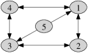
(a)       (b)

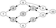
Figure 4.1. (a) A chain graph $\mathcal{G}$ with vertex set $V=\{1,\ldots,5\}$ that has non-decomposable bidirected part. (b) An acyclic digraph $\mathcal{D}$ such that $\mathbf{N}_{V}(\mathcal{D})$ is a full-dimensional subset of $\mathbf{N}(\mathcal{G})$; dashed arrows indicate edges contained in $E_{A}(1,2)$.

Example 4.1.

Let $\mathcal{G}=(V,D,B)$ be the chain graph depicted in Figure 4.1(a). The acyclic digraph $\mathcal{D}=(U,E)$ shown in Figure 4.1(b) is such that $\mathbf{N}_{V}(\mathcal{D})$ is a full-dimensional subset of $\mathbf{N}(\mathcal{G})$. The graph $\mathcal{G}$ has the non-decomposable chain component $C=\{1,\ldots,4\}$, with $A={\rm An}(C)=\{5\}$. In the digraph $\mathcal{D}$, we have $\mathrm{Tops}_{A}(1,2)=\{10,11\}$ and $E_{A}(1,2)=\{10\rightarrow 9,11\rightarrow 1\}$. The two edges in $E_{A}(1,2)$ are represented as dashed arrows in Figure 4.1(b). The corresponding entries in $\Gamma\in\mathbb{R}^{E}$ are negated in the construction of $\Gamma^{\prime}$ in (4.7).

Let $\mathcal{D}_{U\setminus A}$ be the subgraph induced by $U\setminus A$. For a set $Z\subseteq U\setminus A$, we let

$${\rm An}_{U\setminus A}(Z)=\bigcup_{u\in Z}{\rm An}_{U\setminus A}(u)$$

be the ancestors of $Z$ in the induced subgraph $\mathcal{D}_{U\setminus A}$. According to the next lemma, the set of $\mathrm{Tops}_{A}(1,2)$ is ancestral in this induced subgraph. Throughout the rest of the section, d-connecting walks are always d-connecting given $A$.

Lemma 4.4.

The top nodes of d-connecting walks from $1$ to $2$ form an ancestral subset of $\mathcal{D}_{U\setminus A}$, that is,

$${\rm An}_{U\setminus A}\big{(}\mathrm{Tops}_{A}(1,2)\big{)}\subseteq\mathrm{Tops}_{A}(1,2).$$

Proof.

As noted above $\mathrm{Tops}_{A}(1,2)\cap A=\emptyset$. Now suppose that $v\in\mathrm{Tops}_{A}(1,2)$ and there exists a directed path from $u$ to $v$ in $\mathcal{D}_{U\setminus A}$. Choose a d-connecting walk $\pi$ from $1$ to $2$ with $\mathrm{Top}\left({\pi}\right)=v$. At $v$, we may insert into $\pi$, the trek

$$v\leftarrow\cdots\leftarrow u\to\cdots\to v$$

that uses twice the directed path from $u$ to $v$ that exists in $\mathcal{D}_{U\setminus A}$. The insertion yields a walk $\pi^{\prime}$ from $1$ to $2$ that is d-connecting and has $\mathrm{Top}\left({\pi^{\prime}}\right)=u$. ∎

Let $u,v\in[p]$. Using Lemma 3.2, we may write the determinants of $\Sigma_{uA,vA}$ and $\Sigma_{A,A}$ for $\Sigma$ from (4.3) and the analogous determinants for $\Sigma^{\prime}$ from (4.4) as sums over systems of treks without sided intersection. The treks in these systems are thus treks in $\mathcal{D}$ that are formed from two directed paths that do not contain an edge $w\to x$ with source node $w\in A$. We refer to such paths as proper directed paths. If a proper directed path ends with a target node not in $A$ then it is a directed path in the induced subgraph $\mathcal{D}_{U\setminus A}$.

Lemma 4.5.

A proper directed path with a target in $A$ cannot have an edge in $E_{A}(1,2)$.

Proof.

Let $\alpha\in A$, and suppose for contradiction that there exists a proper directed path $\pi$ from a node $u$ to $\alpha$ that contains an edge $v\to w\in E_{A}(1,2)$. Hence,

$$\pi:u\to\cdots\to v\to w\to\cdots\to\alpha.$$

By definition of $E_{A}(1,2)$, we have $w\in{\rm An}_{U\setminus A}(1)$. Thus, there exists a trek $\tau$ in $\mathcal{D}$ of the form

$$\tau:1\leftarrow\cdots\leftarrow w\rightarrow\cdots\rightarrow\alpha$$

that does not have any interior nodes in $A$.

Since $v\in\mathrm{Tops}_{A}(1,2)$ by definition of $E_{A}(1,2)$, it follows from Lemma 4.4 that $u\in\mathrm{Tops}_{A}(1,2)$. Thus there exists a d-connecting walk $\delta$ from 1 to 2 with $u=\mathrm{Top}\left({\delta}\right)$. Define $\delta^{\prime}$ to be the subwalk of $\delta$ from $u$ to 2 formed by removing the directed walk from $u$ to 1 at the beginning of $\delta$. Concatenating $\tau$, the path $\pi$ reversed, and $\delta^{\prime}$ yields a d-connecting walk $\pi^{\prime}$ from 1 to 2 of the form

$$\pi^{\prime}:1\leftarrow\cdots\leftarrow w\rightarrow\cdots\rightarrow\alpha\leftarrow\cdots\leftarrow u\;\cdots\;2$$

that has $w=\mathrm{Top}\left({\mathcal{\pi}^{\prime}}\right)$. Consequently, $w\in\mathrm{Tops}_{A}(1,2)$, contradicting the assumption that $v\to w\in E_{A}(1,2)$. ∎

Lemma 4.6.

A proper directed path with a target in $\{2,\dots,p\}$ cannot have an edge in $E_{A}(1,2)$.

Proof.

Let $x\in\{2,\dots,p\}$, and suppose for contradiction that $v\to w\in E_{A}(1,2)$ is an edge in a proper directed path $\pi$ from a node $u$ to $x$. Written in reverse, $\pi$ is

$$x\leftarrow\cdots\leftarrow w\leftarrow v\leftarrow\cdots\leftarrow u.$$

We distinguish two cases based on whether $x=p$ or not.

If $x\in\{2,\ldots,p-1\}$, then $\mathcal{D}_{U\setminus A}$ contains a trek

$$\tau:1\leftarrow\cdots\leftarrow w\rightarrow\cdots\rightarrow x,$$

since $w\in{\rm An}_{U\setminus A}(1)$. If $x=2$, then $\tau$ is d-connecting and, thus, $w\in\mathrm{Tops}_{A}(1,2)$. This contradicts the assumption that $v\to w\in E_{A}(1,2)$. If $x\in\{3,\ldots,p-1\}$, then $\tau$ is a d-connecting trek between two nodes that are not adjacent in the bidirected cycle $([p],B_{p})$, which is again a contradiction.

Finally, suppose that $x=p$. Since $v\in\mathrm{Tops}_{A}(1,2)$, we also have $u\in\mathrm{Tops}_{A}(1,2)$ by the ancestrality property from Lemma 4.4. Hence, $\mathcal{D}$ contains a d-connecting walk $\delta$ from 1 to 2 such that $u=\mathrm{Top}\left({\delta}\right)$. Define $\delta^{\prime}$ to be the subwalk of $\delta$ from $u$ to 2 formed by removing the directed path from $u$ to 1 at the beginning of $\delta$. Concatenating $\pi$ and $\delta^{\prime}$ yields a walk

$$\pi^{\prime}:p\leftarrow\cdots\leftarrow w\leftarrow v\leftarrow\cdots\leftarrow u\;\cdots\;2,$$

from $p$ to $2$ that is d-connecting. This is a contradiction since $(2,p)\notin B_{p}$. ∎

Lemma 4.7.

Let $\Pi:\{1\}\cup A\rightrightarrows\{2\}\cup A$ be a system of treks without sided intersection, and let $\tau_{1}$ be the trek in $\Pi$ with source 1. Then $\mathrm{Left}\left({\tau_{1}}\right)\neq\{1\}$, $\mathrm{Top}\left({\tau_{1}}\right)\neq 1$, and there is a proper directed path from $\mathrm{Top}\left({\tau_{1}}\right)$ to 1. Moreover, $\mathrm{Top}\left({\tau_{1}}\right)\in\mathrm{Tops}_{A}(1,2)$.

Proof.

Clearly, $1\in\mathrm{Left}\left({\tau_{1}}\right)$. Suppose for contradiction that $\mathrm{Left}\left({\tau_{1}}\right)=\{1\}$. Then $\mathrm{Top}\left({\tau_{1}}\right)=1$, implying that $\tau_{1}$ is a directed path beginning at 1. Appending to $\tau_{1}$ other treks in $\Pi$, we may form a d-connecting walk $\pi$ from $1$ to $2$ that begins with a directed edge $1\to\cdot\,$ pointing away from $1$.

Since $p$ and $1$ are adjacent in the bidirected cycle $([p],B_{p})$, the graph $\mathcal{D}$ contains a d-connecting walk $\pi^{\prime}$ from $p$ to 1. Appending $\pi$ to $\pi^{\prime}$ yields a d-connecting walk $\delta$ from $p$ to 2, which is a contradiction because $(2,p)\not\in B_{p}$. We conclude that $\mathrm{Left}\left({\tau_{1}}\right)\neq\{1\}$, and the other claims are immediate consequences. In particular, $\mathrm{Top}\left({\tau_{1}}\right)=\mathrm{Top}\left({\pi}\right)\in\mathrm{Tops}_{A}(1,2)$. ∎

Lemma 4.8.

A proper directed path with target 1 and source in $\mathrm{Tops}_{A}(1,2)$ has exactly one edge in $E_{A}(1,2)$.

Proof.

First, note that $1\notin\mathrm{Tops}_{A}(1,2)$. Indeed, if $1\in\mathrm{Tops}_{A}(1,2)$, then there is a d-connecting walk from $1$ to $2$ that begins with a directed edge pointing away from $1$. The arguments in the proof of Lemma 4.7 then lead to a contradiction.

Now, let $\pi$ be any proper directed path from a node $u\in\mathrm{Tops}_{A}(1,2)$ to 1. As we traverse $\pi$ from $u$ to 1, there must exist some first node, say $w$, that is not in $\mathrm{Tops}_{A}(1,2)$. Let $v$ be the node that immediately precedes $w$ on $\pi$, and note that $v\in\mathrm{Tops}_{A}(1,2)$. Then $v\to w\in E_{A}(1,2)$.

By Lemma 4.4, $\mathrm{Tops}_{A}(1,2)$ is ancestral with respect to $\mathcal{D}_{U\setminus A}$. Hence, no descendant of $w$ along $\pi$ is in $\mathrm{Tops}_{A}(1,2)$, for else we would have $w\in\mathrm{Tops}_{A}(1,2)$. We conclude that, along $\pi$, every node from $u$ to $v$ is in $\mathrm{Tops}_{A}(1,2)$, and no node from $w$ to 1 is in $\mathrm{Tops}_{A}(1,2)$. Hence, $v\to w$ is the only edge in $\pi$ that is in $E_{A}(1,2)$. ∎

The preceding lemmas yield the following corollary about subdeterminants of the matrices $\Sigma$ and $\Sigma^{\prime}$ from (4.3) and (4.4), respectively.

Corollary 4.9.

The matrices $\Sigma$ and $\Sigma^{\prime}$ from (4.3) and (4.4) satisfy

1. $\det(\Sigma^{\prime}_{A,A})=\det(\Sigma_{A,A})$,

2. $\det(\Sigma^{\prime}_{1A,2A})=-\det(\Sigma_{1A,2A})$, and

3. $\det(\Sigma^{\prime}_{uA,vA})=\det(\Sigma_{uA,vA})$ for all pairs $(u,v)\in([p]\times[p])\setminus\{(1,2),(2,1)\}$.

Proof.

In each case, we may appeal to Lemma 3.2 and consider systems of treks without sided intersection.

(i) Suppose $\Pi:A\rightrightarrows A$ is a system of treks without sided intersection. Since there is no sided intersection, every trek in $\Pi$ must be the concatenation of two proper directed paths, each with target in $A$. By Lemma 4.5, no trek in $\Pi$ contains an edge in $E_{A}(1,2)$. Hence, no trek involves an edge $x\to y$ whose coefficient $\lambda_{xy}$ is negated when replacing $\Sigma$ by $\Sigma^{\prime}$.

(ii) Suppose $\Pi:\{1\}\cup A\rightrightarrows\{2\}\cup A$ is a system of treks without sided intersection. Since there is no sided intersection, every trek in $\Pi$ must be the concatenation of two proper directed paths. Exactly one of these proper directed paths has target 1 and, thus, contains exactly one edge in $E_{A}(1,2)$, by Lemma 4.7 and Lemma 4.8. All other proper directed paths have target in $A$ or target 2. By Lemma 4.5 and Lemma 4.6, none of these paths contains an edge in $E_{A}(1,2)$. We conclude that $\Pi$ contains precisely one edge in $E_{A}(1,2)$. Therefore, its contribution to the sum in Lemma 3.2 is negated when replacing $\Sigma$ by $\Sigma^{\prime}$.

(iii) First, consider the case that $(u,v)\notin\{(1,p),(p,1)\}$. Then all relevant systems of treks without sided intersection are made up of proper directed paths with targets in $A$ or $\{2,\dots,p\}$. By Lemma 4.5 and Lemma 4.6, no edge from $E_{A}(1,2)$ appears in these paths and the claim follows.

Finally, suppose that $(u,v)\in\{(1,p),(p,1)\}$, and let $\Pi:\{u\}\cup A\rightrightarrows\{v\}\cup A$ be a system of treks without sided intersection. Splitting each trek in the system at its top node gives a collection of proper directed paths, of which exactly one path has target node 1. If the source of this path, $x$, is in $\mathrm{Tops}_{A}(1,2)$, then there is a d-connecting walk, $\delta$ from 1 to 2 as well as a d-connecting walk $\delta^{\prime}$ from 1 to $p$ such that $\mathrm{Top}\left({\delta}\right)=\mathrm{Top}\left({\delta^{\prime}}\right)=x$. Traversing $\delta^{\prime}$ backwards from $p$ to $x$ and then traversing $\delta$ from $x$ to 2 traces out a d-connecting walk from $p$ to $2$, which is a contradiction since $p$ and $2$ are not adjacent in the bidirected cycle $([p],B_{p})$. Consequently, the proper directed path with target node 1 does not have its source in $\mathrm{Tops}_{A}(1,2)$. By the ancestrality from Lemma 4.4, none of the edges in this path will be in $E_{A}(1,2)$. Hence, no edge appearing in $\Pi$ has a coefficient that is negated when replacing $\Sigma$ by $\Sigma^{\prime}$. ∎

5. Discussion

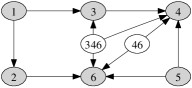
Figure 5.1. A minimal Gaussian causal interpretation for the chain graph $\mathcal{G}$ in Figure 2.1(a). The causality index of $\mathcal{G}$ is 2.

This paper provides a sufficient condition for a mixed graph and its associated Gaussian model to admit a strict causal interpretation in terms of acyclic digraphs with additional nodes that correspond to hidden Gaussian variables. For chain graphs, we show the necessity of the condition. An obvious follow-up problem would be to characterize strict Gaussian causality for more general classes of mixed graphs. The ancestral graphs of [RS02] would be a natural starting point.

If a mixed graph $\mathcal{G}=(V,D,B)$ is strictly Gaussian causal, then there are infinitely many acyclic digraphs $\mathcal{D}=(U,E)$, $U\supseteq V$, that induce a hidden variable model $\mathbf{N}_{V}(\mathcal{D})=\mathbf{N}(\mathcal{G})$. It would be interesting to study just how many hidden variables really need to be introduced for this equality of models. To formalize the question, define the (Gaussian) causality index of a mixed graph to be the minimum number $h$ such that there exists an acyclic digraph $\mathcal{D}$ on nodes $U\supseteq V$ with $|U|=|V|+h$ and $\mathbf{N}_{V}(\mathcal{D})=\mathbf{N}(\mathcal{G})$. If $\mathcal{G}$ is not strictly Gaussian causal, set $h=\infty$. The question is then whether we can efficiently determine the causality index of a general mixed graph. To give an example, the chain graph $\mathcal{G}$ in Figure 2.1(a) has causality index two. Figure 5.1 depicts an acyclic digraph $\mathcal{D}$ with two latent variables that induces a hidden variable model equal to the mixed graph model. For graphs $\mathcal{G}$ with causality index $\infty$ it would furthermore be interesting to determine inequalities that hold on hidden variable models $\mathbf{N}_{V}(\mathcal{D})$ that are full-dimensional subsets of $\mathbf{N}(\mathcal{G})$. The ‘positive definiteness after sign change’ that we use in this paper is one example of such an inequality. For other work on inequality constraints, see [Eva12, KT06] and references therein.

All of the above work considers the concrete setting of hidden variable models that are based on an assumption of joint multivariate normality of all variables, observed and hidden. Alternatively, it would be interesting to treat a non-parametric version of the considered problem. To explain, let $\mathcal{G}=(V,D,B)$ be again a mixed graph with Gaussian model $\mathbf{N}(\mathcal{G})$. For an acyclic digraph $\mathcal{D}=(U,E)$ with $U\supseteq V$ define $\mathbf{P}(\mathcal{D})$ to be set of all probability distributions on $\mathbb{R}^{U}$ that satisfy the conditional independence relations associated with $\mathcal{D}$; compare [Lau96]. Then define $\mathbf{P}_{V}(\mathcal{D})$ to be the set of all distributions on $\mathbb{R}^{V}$ that arise as $V$-marginal of a distribution in $\mathbf{P}(\mathcal{D})$. Writing $\mathbf{N}(V)$ for the set of all multivariate normal distributions on $\mathbb{R}^{V}$ (with positive definite covariance matrix), we may then ask whether

(5.1) $$\mathbf{P}_{V}(\mathcal{D})\cap\mathbf{N}(V)\;=\;\mathbf{N}(\mathcal{G}).$$

While the model $\mathbf{P}(\mathcal{D})$ is certainly much larger than its subset $\mathbf{N}(\mathcal{D})=\mathbf{P}(\mathcal{D})\cap\mathbf{N}(U)$, it is not clear to us that considering the model equality in (5.1) should give anything new. In particular, the Lévy-Cramér theorem [Pol02, §8.8] suggests that when considering structural equations as in (1.2) one would have to consider non-linear equations in order to generate distributions in $\mathbf{P}_{V}(\mathcal{D})\cap\mathbf{N}(V)$ that are not already in $\mathbf{N}_{V}(\mathcal{D})$. If it were the case that a strict causal interpretation cannot always be found via the addition of hidden non-Gaussian variables, then some Gaussian mixed graph models would be larger than needed for modeling of causally induced stochastic dependencies.

References

- [ARS09] R. Ayesha Ali, Thomas S. Richardson, and Peter Spirtes, Markov equivalence for ancestral graphs, Ann. Statist. 37 (2009), no. 5B, 2808–2837.
- [Bol89] Kenneth A. Bollen, Structural equations with latent variables, Wiley Series in Probability and Mathematical Statistics: Applied Probability and Statistics, John Wiley & Sons Inc., New York, 1989, A Wiley-Interscience Publication. MR996025 (90k:62001)
- [CMKR12] Diego Colombo, Marloes H. Maathuis, Markus Kalisch, and Thomas S. Richardson, Learning high-dimensional directed acyclic graphs with latent and selection variables, Ann. Statist. 40 (2012), no. 1, 294–321.
- [DER09] Mathias Drton, Michael Eichler, and Thomas S. Richardson, Computing maximum likelihood estimates in recursive linear models with correlated errors, J. Mach. Learn. Res. 10 (2009), 2329–2348.
- [DFS11] Mathias Drton, Rina Foygel, and Seth Sullivant, Global identifiability of linear structural equation models, Ann. Statist. 39 (2011), no. 2, 865–886.
- [DR08] Mathias Drton and Thomas S. Richardson, Graphical methods for efficient likelihood inference in Gaussian covariance models, J. Mach. Learn. Res. 9 (2008), 893–914. MR996025 (90k:62001)
- [Drt09] Mathias Drton, Discrete chain graph models, Bernoulli 15 (2009), no. 3, 736–753. MR996025 (90k:62001)
- [DSS09] Mathias Drton, Bernd Sturmfels, and Seth Sullivant, Lectures on algebraic statistics, Oberwolfach Seminars, vol. 39, Birkhäuser Verlag, Basel, 2009. MR996025 (90k:62001)
- [DY10] Mathias Drton and Josephine Yu, On a parametrization of positive semidefinite matrices with zeros, SIAM J. Matrix Anal. Appl. 31 (2010), no. 5, 2665–2680. MR996025 (90k:62001)
- [Eva12] Robin J. Evans, Graphical methods for inequality constraints in marginalized DAGs, IEEE International Workshop on Machine Learning for Signal Processing (I. Santamaria, J. Arenas-Garcia, G. Camps-Valls, D. Erdogmus, F. Perez-Cruz, and J. Larsen, eds.), September 2012, pp. 574–579, arXiv:1209.2978.
- [Kos99] Jan T. A. Koster, On the validity of the Markov interpretation of path diagrams of Gaussian structural equations systems with correlated errors, Scand. J. Statist. 26 (1999), no. 3, 413–431.
- [Kos02] by same author, Marginalizing and conditioning in graphical models, Bernoulli 8 (2002), no. 6, 817–840.
- [KT06] Changsung Kang and Jin Tian, Inequality constraints in causal models with hidden variables, Proceedings of the Twenty-Second Conference Annual Conference on Uncertainty in Artificial Intelligence (UAI-06) (Arlington, Virginia), AUAI Press, 2006, pp. 233–240.
- [Lau96] Steffen L. Lauritzen, Graphical models, Oxford Statistical Science Series, vol. 17, The Clarendon Press Oxford University Press, New York, 1996, Oxford Science Publications. MR996025 (90k:62001)
- [Pea09] Judea Pearl, Causality, second ed., Cambridge University Press, Cambridge, 2009, Models, reasoning, and inference. MR996025 (90k:62001)
- [Pol02] David Pollard, A user’s guide to measure theoretic probability, Cambridge Series in Statistical and Probabilistic Mathematics, vol. 8, Cambridge University Press, Cambridge, 2002. MR996025 (90k:62001)
- [PW94] Judea Pearl and Nanny Wermuth, When can association graphs admit a causal interpretation?, Selecting Models from Data: Artificial Intelligence and Statistics IV, Lecture Notes in Statistics, vol. 89, Springer, New York, 1994, pp. 205–214.
- [RS02] Thomas Richardson and Peter Spirtes, Ancestral graph Markov models, Ann. Statist. 30 (2002), no. 4, 962–1030. MR996025 (90k:62001)
- [SG09] Ricardo Silva and Zoubin Ghahramani, The hidden life of latent variables: Bayesian learning with mixed graph models, J. Mach. Learn. Res. 10 (2009), 1187–1238. MR996025 (90k:62001)
- [SGS00] Peter Spirtes, Clark Glymour, and Richard Scheines, Causation, prediction, and search, second ed., Adaptive Computation and Machine Learning, MIT Press, Cambridge, MA, 2000, With additional material by David Heckerman, Christopher Meek, Gregory F. Cooper and Thomas Richardson, A Bradford Book. MR996025 (90k:62001)
- [STD10] Seth Sullivant, Kelli Talaska, and Jan Draisma, Trek separation for Gaussian graphical models, Ann. Statist. 38 (2010), no. 3, 1665–1685. MR996025 (90k:62001)
- [WC04] Nanny Wermuth and D. R. Cox, Joint response graphs and separation induced by triangular systems, J. R. Stat. Soc. Ser. B Stat. Methodol. 66 (2004), no. 3, 687–717. MR996025 (90k:62001)
- [Wer11] Nanny Wermuth, Probability distributions with summary graph structure, Bernoulli 17 (2011), no. 3, 845–879. MR996025 (90k:62001)
- [Wri21] Sewall Wright, Correlation and causation, J. Agricultural Research 20 (1921), 557–585.
- [Wri34] by same author, The method of path coefficients, Ann. Math. Statist. 5 (1934), no. 3, 161–215.
- [WS12] Nanny Wermuth and Kayvan Sadeghi, Sequences of regressions and their independences, TEST 21 (2012), no. 2, 215–252. MR996025 (90k:62001)
- [ZZL05] Hui Zhao, Zhongguo Zheng, and Baijun Liu, On the Markov equivalence of maximal ancestral graphs, Sci. China Ser. A 48 (2005), no. 4, 548–562. MR996025 (90k:62001)