Sailfish: Alignment-free Isoform Quantification from RNA-seq Reads using Lightweight Algorithms

RNA-seq has rapidly become the de facto technique to measure gene expression. However, the time required for analysis has not kept up with the pace of data generation. Here we introduce Sailfish, a novel computational method for quantifying the abundance of previously annotated RNA isoforms from RNA-seq data. Sailfish entirely avoids mapping reads, which is a time-consuming step in all current methods. Sailfish provides quantification estimates much faster than existing approaches (typically 20-times faster) without loss of accuracy.

The ability to generate genomic and transcriptomic data is accelerating beyond our ability to process it. The increasingly widespread use and growing clinical relevance (e.g. [11]) of RNA-seq measurements of transcript abundance will only serve to magnify the divide between our data acquisition and data analysis capabilities.

The goal of isoform quantification is to determine the relative abundance of different RNA transcripts given a set of RNA-seq reads. In the analysis of RNA-seq data, isoform quantification is one of the most computationally time-consuming steps, and it is commonly the first step in an analysis of differential expression among multiple samples [13]. There are numerous computational challenges in estimating transcript-level abundance from RNA-seq data. Mapping the sequencing reads to the genome or transcript sequences can require substantial computational resources. This often leads to complicated models that account for read bias and error during inference, further adding to the time spent on analysis. Finally, some reads, known as multireads [7, 15], can map to multiple, sometimes many, different transcripts. The ambiguity resulting from these multireads complicates the estimation of relative transcript abundances.

Existing approaches first use read-mapping tools, such as Bowtie [4], to determine potential locations from which the RNA-seq reads originated. Given the read alignments, some of the most accurate transcript quantification tools resolve the relative abundance of transcripts using expectation-maximization (EM) procedures [15, 5, 10]. In such procedures, reads are first assigned to transcripts, and these assignments are then used to estimate transcript abundances. The abundances are then used to re-estimate the read assignments, weighting potential matches in proportion to the currently estimated relative abundances, and these steps are repeated until convergence. In practice, both of these steps can be time consuming. For example, even when exploiting the parallel nature of the problem, mapping the reads from a reasonably sized (e.g. 100M reads) RNA-seq experiment can take hours.

Recent tools, such as eXpress [10], aim to reduce the computational burden of isoform quantification from RNA-seq data by substantially altering the EM algorithm. However, even for such advanced approaches, performing read alignment and processing the large number of alignments that result from ambiguously mapping reads remains a significant bottleneck and fundamentally limits the scalability of approaches that depend on mapping.

Sailfish, our software for isoform quantification from RNA-seq data, is based on the philosophy of lightweight algorithms, which make frugal use of data, respect constant factors, and effectively use concurrent hardware by working with small units of data where possible. Sailfish avoids mapping reads entirely (Fig. 1), resulting in large savings in time and space. A key technical contribution behind our approach is the observation that transcript coverage, which is essential for isoform quantification, can be reliably and accurately estimated using counts of k-mers occurring in reads. This results in the ability to obtain accurate quantification estimates more than an order of magnitude faster than existing approaches, often in minutes instead of hours. For example, for the data described in Figure LABEL:fig:results, Sailfish is between 18 and 29 times faster than the next fastest method while providing expression estimates of equal accuracy.

In Sailfish, the fundamental unit of transcript coverage is the k-mer. This is different from existing approaches, where the fragment or read is the fundamental unit of coverage. By working with k-mers, we can replace the computationally intensive step of read mapping with the much faster and simpler process of k-mer counting. We also avoid any dependence on read mapping parameters (e.g. mismatches and gaps) that can have a significant effect on both the runtime and accuracy of conventional approaches. Yet, our approach is still able to handle sequencing errors in reads because only the k-mers that overlap the erroneous bases will be discarded or mis-assigned, while the rest of the read can be processed as if it were error-free. This also leads to Sailfish having only a single explicit parameter, the k-mer length. Longer k-mers may result in less ambiguity, which makes resolving their origin easier, but may be more affected by errors in the reads. Conversely, shorter k-mers, though more ambiguous, may be more robust to errors in the reads (Supplementary Fig. 1). Further, we can effectively exploit modern hardware where multiple cores and reasonably large memories are common. Many of our data structures can be represented as arrays of atomic integers (see Methods). This allows our software to be concurrent and lock-free where possible, leading to an approach that scales well with the number of available CPUs (Supplementary Fig. 2). Additional benefits of the Sailfish approach are discussed in Supplementary Note 1.

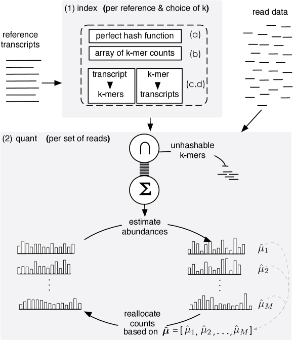
Figure 1: The Sailfish pipeline consists of an indexing phase (1) that is invoked via the command sailfish index and a quantification phase (2) invoked via the command sailfish quant. The Sailfish index has four components: (a) a perfect hash function mapping each k-mer in the transcript set to a unique integer between $0$ and $N$ — the number of unique k-mers in the set of transcripts; (b) an array recording the number of times each k-mer occurs in the reference set; (c) an index mapping each transcript to the multiset of k-mers that it contains; (d) an index mapping each k-mer to the set of transcripts in which it appears. The quantification phase consists of counting the indexed k-mers in the set of reads and then applying an EM procedure to determine the maximum-likelihood estimates of relative transcript abundance.

Sailfish works in two phases: indexing and quantification (Fig. 1). A Sailfish index is built from a particular set of reference transcripts (a FASTA sequence file) and a specific choice of k-mer length, $k$. The index consists of data structures that make counting k-mers in a set of reads and resolving their potential origin in the set of transcripts efficient (see Methods). The most important data structure in the index is the minimal perfect hash function [1] that maps each k-mer in the reference transcripts to an index between $0$ and the number of different k-mers in the transcripts such that no two k-mers share an index. This allows us to quickly index and count any k-mer from the reads that also appears in the transcripts. We find that pairing the minimum perfect hash function with an atomically updateable array of k-mer counts allows us to count k-mers even faster than with existing advanced lock-free hashes such as that used in Jellyfish [6]. The index also contains a pair of look-up tables that allow fast access to the indexed k-mers appearing in a specific transcript as well as the indexed transcripts in which a particular k-mer appears, both in amortized constant time. Because the index depends only on the set of reference transcripts and the choice of k-mer length, it only needs to be rebuilt when one of these factors changes.

The quantification phase of Sailfish takes as input the index described above and a set of RNA-seq reads and produces an estimate of the relative abundance of each transcript in the reference, measured in both Reads Per Kilobase per Million mapped reads (RPKM) and Transcripts Per Million (TPM); (see Methods for the definitions of these measures). First, Sailfish counts the number of times each indexed k-mer occurs in the set of reads. Owing to efficient k-mer indexing by means of the perfect hash function and the use of a lock-free counting data structure (Methods), this process is efficient and scalable (Supplementary Fig. 2). Sailfish then applies an expectation-maximization (EM) procedure to determine maximum likelihood estimates for the relative abundance of each transcript. Conceptually, this procedure is similar to the EM algorithm used by RSEM [5], except that k-mers rather than fragments are probabilistically assigned to transcripts, and a two-step variant of EM is used to speed up convergence. The estimation procedure first assigns k-mers proportionally to transcripts (i.e. if a transcript is the only potential origin for a particular k-mer, then all observations of that k-mer are attributed to this transcript, whereas for a k-mer that appears once in each of $n$ different transcripts and occurs $m$ times in the set of reads, $m/n$ observations are attributed to each potential transcript of origin). These initial allocations are then used to estimate the expected coverage for each transcript (Methods, Eqn. 3). In turn, these expected coverage values alter the assignment probabilities of k-mers to transcripts (Methods, Eqn. 1). Using these basic EM steps as a building block, we apply a globally-convergent EM acceleration method, SQUAREM [16], that substantially increases the convergence rate of the estimation procedure by modifying the parameter update step and step-length based on the current solution path and the estimated distance from the fixed point (see Methods, Alg. 2).

Additionally, we reduce the number of variables that need to be fit by the EM procedure by collapsing k-mers into equivalence classes. Two k-mers are equivalent from the perspective of the EM algorithm if they occur in the same set of transcript sequences with the same rate (more details available in Methods). This reduction in the number of active variables substantially reduces the computational requirements of the EM procedure. For example, in the set of reference transcripts for which we estimate abundance using the Microarray Quality Control (MAQC) [12] data (Fig. LABEL:fig:results), there are $60504111$ k-mers ($k=20$), of which $39393132$ appear at least once in the set of reads. However, there are only $151385$ distinct equivalence classes of k-mers with non-zero counts. Thus, our EM procedure needs to optimize the allocations of $151385$ k-mer equivalence classes instead of $39393132$ individual k-mers, a reduction by a factor of $\approx 260$.

Once the EM procedure converges, the estimated abundances are corrected for systematic errors due to sequence composition bias and transcript length using a regression approach similar to Zheng et al. [18], though using random forest regression instead of a generalized additive model. This correction is applied after initial estimates have been produced rather than at a read mapping or fragment assignment stage, requiring fewer variables to be fit during bias correction.

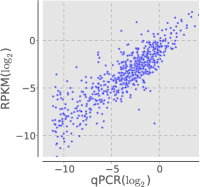
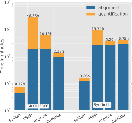
a	c
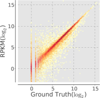
b

	Human Brain Tissue				Synthetic
	Sailfish	RSEM	eXpress	Cufflinks	Sailfish	RSEM	eXpress	Cufflinks
Pearson	0.86	0.83	0.86	0.86	0.92	0.92	0.64	0.91
Spearman	0.85	0.81	0.86	0.86	0.94	0.93	0.66	0.93
RMSE	1.69	1.86	1.69	1.67	1.26	1.24	2.80	1.31
medPE	31.60	36.63	32.73	30.75	4.24	5.97	26.44	6.76

d

Figure 2: (a) The correlation between qPCR estimates of gene abundance (x-axis) and the estimates of Sailfish. The ground-truth results are taken from the microarray quality control study (MAQC) [12]. The results shown here are for the human brain tissue and the RNA-seq based estimates were computed using the reads from SRA accession SRX016366. The set of transcripts used in this experiment were the curated RefSeq [9] genes (accession prefix NM) from hg18. (b) The correlation between the actual number of transcript copies in a simulated dataset (x-axis) and the abundance estimates of Sailfish. The transcripts used in this experiment were all Ensembl [2] transcripts from hg19 that were annotated with a coding feature (CDS). (c) The total time taken by each method, Sailfish, RSEM, eXpress and Cufflinks, to estimate isoform abundance on each dataset. The total time taken by a method is the height of the corresponding bar, and the total is further broken down into the time taken to perform read-alignment (for Sailfish, we instead measured the time taken to count the k-mers in the read set) and the time taken to quantify abundance given the aligned reads (or k-mer counts). All tools were run in multi-threaded mode (where applicable) and were allowed to use up to $16$ threads. The table (d) gives the accuracy of each of the methods on both datasets, as measured by the Pearson and Spearman correlation coefficients, root-mean-square error (RMSE) and median percentage error (medPE).

To examine the efficiency and accuracy of Sailfish, we compared it to RSEM [5], eXpress [10] and Cufflinks [15] using both real and synthetic data. Accuracy on real data was quantified by the agreement between RNA-seq-based expression estimates computed by each piece of software and qPCR measurements for the same sample (human brain tissue (HBR) in Fig. LABEL:fig:results and Supplementary Fig. 3, and universal human reference tissue (UHR) in Supplementary Fig. 4). These paired RNA-seq and qPCR experiments were performed as part of the Microarray Quality Control (MAQC) study [12]. qPCR abundance measurements are given at the resolution of genes rather than isoforms. Thus, to compare these measurements with the transcript-level abundance estimates produced by the software, we summed the estimates for all isoforms belonging to a gene to obtain an estimate for that gene. We compare predicted abundances using correlation coefficients, root-mean-square error (RMSE), and median percentage error (medPE) (additional details available in Supplementary Note 2). Figure LABEL:fig:results shows that the speed of Sailfish does not sacrifice any accuracy.

To show that Sailfish is accurate at the isoform level, we generated synthetic data using the Flux Simulator [3], which allows versatile modeling of various RNA-seq protocols (see Supplementary Note 3). Unlike synthetic test data used in previous work [5, 10], the procedure used by the Flux Simulator is not based specifically on the generative model underlying our estimation procedure. Sailfish remains accurate at the isoform level (Fig. LABEL:fig:results).

The memory usage of Sailfish is comparable with that of other tools, using between 4 and 6 Gb of RAM during isoform quantification for the experiments reported here.

Sailfish applies the idea of lightweight algorithms to the problem of isoform quantification from RNA-seq reads and in doing so achieves a breakthrough in terms of speed. By eliminating the necessity of read mapping from the expression estimation pipeline, we not only improve the speed of the process but also simplify it considerably, eliminating the burden of choosing all but a single external parameter (the k-mer length) from the user. As the size and number of RNA-seq experiments grow, we expect Sailfish and its paradigm to remain efficient for isoform quantification because the memory footprint is bounded by the size and complexity of the target transcripts and the only phase that grows explicitly in the number of reads — k-mer counting — has been designed to effectively exploit many CPU cores.

Sailfish is free and open-source software and is available at http://www.cs.cmu.edu/~ckingsf/software/sailfish.

Methods

Indexing.

The first step in the Sailfish pipeline is building an index from the set of reference transcripts $\mathcal{T}$. Given a k-mer length $k$, we compute an index $I_{k}({\mathcal{T}})$ containing four components. The first component is a minimum perfect hash function $h$ on the set of k-mers $\textrm{{kmers}}(\mathcal{T})$ contained in $\mathcal{T}$. A minimum perfect hash function is a bijection between $\textrm{{kmers}}(\mathcal{T})$ and the set of integers $\{0,1,\dots,\left|\textrm{{kmers}}(\mathcal{T})\right|-1\}$. Sailfish uses the BDZ minimum perfect hash function [1]. The second component of the index is an array $C$ containing a count $C\left(s_{i}\right)$ for every $s_{i}\in\textrm{{kmers}}(\mathcal{T})$. Finally, the index contains a lookup table $F$, mapping each transcript to the multiset of k-mers that it contains and a reverse lookup table $R$ mapping each k-mer to the set of transcripts in which it appears. The index is a product only of the reference transcripts and the choice of $k$, and thus needs only to be recomputed when either of these changes.

Quantification.

The second step in the Sailfish pipeline is the quantification of relative transcript abundance; this requires the Sailfish index $I_{k}({\mathcal{T}})$ for the reference transcripts $\mathcal{T}$ as well as a set of RNA-seq reads $\mathcal{R}$. First, we count the number of occurrences of each $s_{i}\in\textrm{{kmers}}(\mathcal{T})\cap\textrm{{kmers}}(\mathcal{R})$. Since we know exactly the set of k-mers that need to be counted and already have a perfect hash function $h$ for this set, we can perform this counting in a particularly efficient manner. We maintain an array $C_{\mathcal{R}}$ of the appropriate size $\left|\textrm{{kmers}}(\mathcal{T})\right|$, where $C_{\mathcal{R}}\left(h(s_{i})\right)$ contains the number of times we have thus far observed $s_{i}$ in $\mathcal{R}$.

Sequencing reads, and hence the k-mers they contain, may originate from transcripts in either the forward or reverse direction. To account for both possibilities, we check both the forward and reverse-complement k-mers from each read and use a majority-rule heuristic to determine which of the k-mers to increment in the final array of counts $C_{\mathcal{R}}$. If the number of k-mers appearing in $h$ from the forward direction of the read is greater than the number of reverse-complement k-mers, then we only increment the counts for k-mers appearing in this read in the forward direction. Otherwise, only counts for k-mers appearing in the reverse-complement of this read are incremented in the array of counts. Ties are broken in favor of the forward directed reads. By taking advantage of atomic integers and the compare-and-swap (CAS) operation provided by modern processors, which allows many hardware threads to efficiently update the value of a memory location without the need for explicit locking, we can stream through $\mathcal{R}$ and update the counts of $C_{\mathcal{R}}$ in parallel while sustaining very little resource contention.

We then apply an expectation-maximization algorithm to obtain estimates of the relative abundance of each transcript. We define a k-mer equivalence class as the set of all k-mers that appear in the same set of transcripts with the same frequency. In other words, let $\chi(s)$ be a vector that so that entry $t$ of $\chi(s)$ gives how many times $s$ appears in transcript $t\in\mathcal{T}$. Then the equivalence class of a k-mer $s_{i}$ is given by $\left[s_{i}\right]=\{s_{j}\in\textrm{{kmers}}(\mathcal{T})\mid\chi(s_{j})=\chi(s_{i})\}$. When performing the EM procedure, we will allocate counts to transcripts according to the set of equivalence classes rather than the full set of transcripts. We will let $T(\left[s_{i}\right])=\sum_{s_{j}\in\left[s_{i}\right]}C_{\mathcal{R}}\left(h(s_{j})\right)$ denote the total count of k-mers in $\mathcal{R}$ that originate from equivalence class $\left[s_{i}\right]$. We say that transcript $t$ contains equivalence class $\left[s\right]$ if $\left[s\right]$ is a subset of the multiset of k-mers of $t$ and denote this by $\left[s\right]\subseteq t$.

Estimating abundances via an EM algorithm.

The EM algorithm (Algo. 1) alternates between estimating the fraction of counts of each observed k-mer that originates from each transcript (E-step) and estimating the relative abundances of all transcripts given this allocation (M-step).

The E-step of the EM algorithm computes the fraction of each k-mer equivalence class’ total count that is allocated to each transcript. For equivalence class $\left[s_{j}\right]$ and transcript $t_{i}$, this value is computed by

$$\alpha(j,i)=\frac{\hat{\mu}_{i}T(\left[s_{j}\right])}{\sum_{t\supseteq\left[s_{j}\right]}\hat{\mu}_{t}},$$ (1)

where $\hat{\mu}_{i}$ is the currently estimated relative abundance of transcript $i$. These allocations are then used in the M-step of the algorithm to compute the relative abundance of each transcript. The relative abundance of transcript $i$ is estimated by

$$\hat{\mu}_{i}=\frac{\mu_{i}}{\sum_{t_{j}\in\mathcal{T}}\mu_{j}},$$ (2)

where $\mu_{i}$ is

$$\mu_{i}=\frac{\sum_{\left[s_{j}\right]\subseteq t_{i}}\alpha(j,i)}{\hat{l_{i}}}.$$ (3)

The variable $\hat{l_{i}}$ denotes the adjusted length of transcript $i$ and is simply $\hat{l_{i}}=l_{i}-k+1$ where $l_{i}$ is the length of transcript $i$ in nucleotides.

1 function EM($\bm{\hat{\mu}}$)

2 begin

3       for $\left[s_{j}\right]$ do

4             $w=\sum_{t\supseteq\left[s_{j}\right]}\hat{\mu}_{t}$

5             for $t\supseteq\left[s_{j}\right]$ do

6                   $\alpha(j,i)=\hat{\mu}_{i}T(\left[s_{j}\right])/w$

7                  

8            

9      

10      $y=0$

11       for $t\in\mathcal{T}$ do

12             $C_{t}=\sum_{\left[s_{j}\right]\subseteq t_{i}}\alpha(j,i)$

13             $\mu^{\prime}_{t}=C_{t}/\hat{l_{i}}$

14             $y=y+\mu_{t}$

15            

16      

17      for $t\in\mathcal{T}$ do

18             $\hat{\mu^{\prime}}_{t}=\mu^{\prime}_{t}/y$

19            

20      

21      return $\bm{\hat{\mu^{\prime}}}=\langle\bm{\hat{\mu^{\prime}}}_{0},\bm{\hat{\mu^{\prime}}}_{1},\dots,\bm{\hat{\mu^{\prime}}}_{\left|\mathcal{T}\right|}\rangle$

22      

23

Algorithm 1 An EM iteration. One iteration of the expectation-maximization procedure that updates the estimated k-mer allocations $\alpha(\cdot,\cdot)$ and computes new estimates of relative transcript abundance $\bm{\hat{\mu^{\prime}}}$ based on the current estimates of relative transcript abundance $\bm{\hat{\mu}}$.

1 $\bm{\hat{\mu}}_{1}=\mathrm{EM}(\bm{\hat{\mu}}_{0})$

2 $\bm{\hat{\mu}}_{2}=\mathrm{EM}(\bm{\hat{\mu}}_{1})$

3 $r=\bm{\hat{\mu}}_{1}-\bm{\hat{\mu}}_{0}$

4 $v=(\bm{\hat{\mu}}_{2}-\bm{\hat{\mu}}_{1})-r$

5 $\gamma=-\left|\left|r\right|\right|/\left|\left|v\right|\right|$

6 modify $\gamma$ by backtracking, if necessary, to ensure global convergence

7 $\bm{\hat{\mu}}_{3}=\max(\bm{0},\bm{\hat{\mu}}_{0}-2\gamma r+\gamma^{2}v)$

8 $\bm{\hat{\mu}}_{0}=\mathrm{EM}(\bm{\hat{\mu}}_{3})$

Algorithm 2 A SQUAREM iteration. Updates the relative abundance estimates according to an accelerated EM procedure whose update direction and magnitude are dynamically computed [16].

However, rather than perform the standard EM update steps, we perform updates according to the SQUAREM procedure [16] described in Algo. 2. $\bm{\hat{\mu}}_{t}=\langle\hat{\mu}_{0},\dots,\hat{\mu}_{\left|\mathcal{T}\right|}\rangle$ is a vector of relative abundance maximum-likelihood estimates, and $\textrm{EM}(\cdot)$ is a standard iteration of the expectation-maximization procedure as outlined in Algo. 1. For a detailed explanation of the SQUAREM procedure and its proof of convergence, see [16]. Intuitively, the SQUAREM procedure builds an approximation of the Jacobian of $\bm{\hat{\mu}}$ from $3$ successive steps along the EM solution path, and uses the magnitude of the differences between these solutions to determine a step size $\gamma$ by which to update the estimates according to the update rule (line 2). The procedure is then capable of making relatively large updates to the $\bm{\hat{\mu}}$ parameters, which substantially improves the speed of convergence. In Sailfish, the iterative SQUAREM procedure is repeated for a user-specified number of steps ($30$ for all experiments reported in this paper; see Supplementary Fig. 5).

Bias Correction.

The bias correction procedure implemented in Sailfish is based on the model introduced by Zheng et al. [18]. Briefly, it performs a regression analysis on a set of potential bias factors where the response variables are the estimated transcript abundances (RPKMs). Sailfish automatically considers transcript length, GC content and dinucleotide frequencies as potential bias factors, as this specific set of features were suggested by Zheng et al. [18]. For each transcript, the prediction of the regression model represents the contribution of the bias factors to this transcript’s estimated abundance. Hence, these regression estimates (which may be positive or negative) are subtracted from the original estimates to obtain bias-corrected RPKMs. For further details on this bias correction procedure, see [18]. The original method used a generalized additive model for regression; Sailfish implements the approach using random forest regression to leverage high-performance implementations of this technique. The key idea here is to do the bias correction after abundance estimation rather than earlier in the pipeline. The bias correction of Sailfish can be disabled with the --no-bias-correction command line option. Finally, we note that it is possible to include other potential features, like normalized coverage plots that can encode positional bias, into the bias correction phase. However, in the current version of Sailfish, we have not implemented or tested bias correction for these features.

Computing RPKM and TPM.

Sailfish outputs both Reads Per Kilobase per Million mapped reads (RPKM) and Transcripts Per Million (TPM) as quantities predicting the relative abundance of different isoforms. The RPKM estimate is the most commonly used, and is ideally $10^{9}$ times the rate at which reads are observed at a given position, but the TPM estimate has also become somewhat common [5, 17]. Given the relative transcript abundances $\hat{\mu_{i}}$ estimated by the EM procedure described above, the TPM for transcript $i$ is given by

$$\textrm{TPM}_{i}=10^{6}\hat{\mu}_{i}.$$ (4)

Let $C_{i}=\sum_{\left[s_{j}\right]\subseteq t_{i}}\alpha(j,i)$ be the number of k-mers mapped to transcript $i$. Then, the RPKM is given by

$$\textrm{RPKM}_{i}=\frac{\frac{C_{i}}{\nicefrac{{l_{i}}}{{10^{3}}}}}{\frac{N}{10^{6}}}=\frac{10^{9}\frac{C_{i}}{l_{i}}}{N}\approx\frac{10^{9}\mu_{i}}{N},$$ (5)

where $N=\sum_{\left[s_{i}\right]}T(\left[s_{i}\right])$ and the final equality is approximate only because we replace $l_{i}$ with $\hat{l_{i}}$.

Computing Accuracy Metrics.

Since the RPKM (and TPM) measurements are only relative estimates of isoform abundance, it is essential to put the ground-truth and estimated relative abundances into the same frame of reference before computing our validation statistics. While this centering procedure will not effect correlation estimates, it is important to perform before computing RMSE and medPE. Let $X=\{x_{i}\}_{i=1}^{M}$ denote the ground-truth isoform abundances and $Y=\{y_{i}\}_{i=1}^{M}$ denote the estimated abundances. We transform the estimated abundances by aligning their centroid with that of the ground-truth abundances; specifically, we compute the centroid-adjusted abundance estimates as $Y^{\prime}=\{y_{i}-\omega\}_{i=1}^{M}$ where $\omega=\left(\sum_{i=i}^{M}x_{i}-\sum_{i=1}^{M}y_{i}\right)/M$. It is these centroid adjusted abundance estimates on which we compute all statistics.

Simulated Data.

The simulated RNA-seq data was generated by the FluxSimulator [3] v1.2 with the parameters listed in Supplementary Note 3. This resulted in a dataset of $150$M, 76 base-pair pared-end reads. RSEM, eXpress and Cufflinks were given paired-end alignments since they make special use of this data. Further, for this dataset, Bowtie [4] was given the additional flag -X990 when aligning the reads to the transcripts, as $990$ base-pairs was the maximum observed insert size in the simulated data. TopHat [14] was provided with the option --mate-inner-dist 198, to adjust the expected mate-pair inner-distance to the simulated average. The read files were provided directly to Sailfish without any extra information since the same quantification procedure is used whether single or paired end reads are provided.

Software Comparisons.

For all comparisons, both eXpress and RSEM were provided with the same sets of aligned reads in BAM format. All reads were aligned with Bowtie [4] v0.12.9 using the parameters -aS and -v3, which allows up to three mismatches per read and reports all alignments. To prepare an alignment for Cufflinks, TopHat was run using Bowtie 1 (--bowtie1) and with options -N 3 and --read-edit-dist 3 to allow up to three mismatches per read. For RSEM, eXpress and Cufflinks, the reported times were the sum of the times required for alignment (via Bowtie for RSEM and eXpress or via TopHat for Cufflinks) and the times required for quantification. The time required for each method is further decomposed into the times for the alignment and quantification steps in Fig. LABEL:fig:results.

Choice of Software Options and Effect on Runtime.

Most expression estimation software, including RSEM, eXpress and Cufflinks, provides a myriad of program options to the user which allow for trade-offs between various desiderata. For example, the total time required by TopHat and Cufflinks is lower when Cufflinks is run without bias correction (e.g. $1.92$h as opposed to $2.27$h with bias correction on the SRX016366 data). However, without bias correction, Cufflinks yields slightly lower accuracy (Pearson $\sigma=0.82$, Spearman $\rho=0.81$) than the other methods, while still taking $16$ times longer to run than Sailfish. Similarly, although aligned reads can be streamed directly into eXpress via Bowtie, we empirically observed lower overall runtimes when aligning reads and quantifying expressions separately (and in serial), so these times were reported. Also, we found that on the synthetic data, the correlations produced by eXpress improved to Pearson $\sigma=0.85$, Spearman $\rho=0.87$ and $\sigma=0.9$, $\rho=0.92$ when running the EM procedure for 10 or 30 extra rounds (-b 10 and -b 30). However, this also greatly increased the runtime (just for the estimation step) from 1.9h to 16.71h and 42.12h respectively. In general, we attempted to run each piece of software with the options that would be most common in a standard usage scenario. However, despite the inherent difficulty of comparing a set of tools parameterized on an array of potential options, the core thesis that Sailfish can provide accurate expression estimates much faster than any existing tool remains true, as the fastest performing alternatives, when even when sacrificing accuracy for speed, were over an order of magnitude slower than Sailfish.

Sailfish version 0.5 was used for all experiments, and all analyses were performed with a k-mer size of $k=20$. Bias correction was enabled in all experiments involving real but not simulated data. The RPKM values reported by Sailfish were used as transcript abundance estimates.

RSEM [5] version 1.2.3 was used with default parameters, apart from being provided the alignment file (--bam), for all experiments, and the RPKM values reported by RSEM were used as abundance estimates.

eXpress [10] version 1.3.1 was used for all experiments. It was run with default parameters on the MACQ data, and without bias correction (--no-bias-correct) on the synthetic data. The abundance estimates were taken as the FPKM values output by eXpress.

Cufflinks [15] version 2.1.1 was used for experiments and was run with bias correction (-b) and multi-read recovery (-u) on the MACQ data, and with only multi-read recovery (-u) on the synthetic data. The FPKM values output by Cufflinks were used as the transcript abundance estimates.

All experiments were run on a computer with 8 AMD Opteron^TM 6220 processors (4 cores each) and 256Gb of RAM. For all experiments, the wall time was measured using the built-in bash time command.

Implementation of Sailfish.

Sailfish has two basic subcommands, index and quant. The index command initially builds a hash of all k-mers in the set of reference transcripts using the Jellyfish [6] software. This hash is then used to build the minimum perfect hash, count array, and look-up tables described above. The index command takes as input a k-mer size via the -k option and a set of reference transcripts in FASTA format via the -t parameter. It produces the Sailfish index described above, and it can optionally take advantage of multiple threads with the target number of threads being provided via a -p option.

The quant subcommand estimates the relative abundance of transcripts given a set of reads. The quant command takes as input a Sailfish index (computed via the index command described above and provided via the -i parameter). Additionally, it requires the set of reads, provided as a list of FASTA or FASTQ files given by the -r parameter. Finally, just as in index command, the quant command can take advantage of multiple processors, the target number of which is provided via the -p option.

Sailfish is implemented in C++11 and takes advantage of several C++11 language and library features. In particular, Sailfish makes heavy use of built-in atomic data types. Parallelization across multiple threads in Sailfish is accomplished via a combination of the standard library’s thread facilities and the Intel Threading Building Blocks (TBB) library [8]. Sailfish is available as an open-source program under the GPLv3 license, and has been developed and tested on Linux and Macintosh OS X.

Author Contributions

R.P., S.M.M. and C.K. designed the method and algorithms, devised the experiments, and wrote the manuscript. R.P. implemented the Sailfish software.

Acknowledgments

This work has been partially funded by National Science Foundation (CCF-1256087, CCF-1053918, and EF-0849899) and National Institutes of Health (1R21AI085376 and 1R21HG006913). C.K. received support as an Alfred P. Sloan Research Fellow.

Supplementary Figure 1: Effect of k-mer length on retained data and k-mer ambiguity

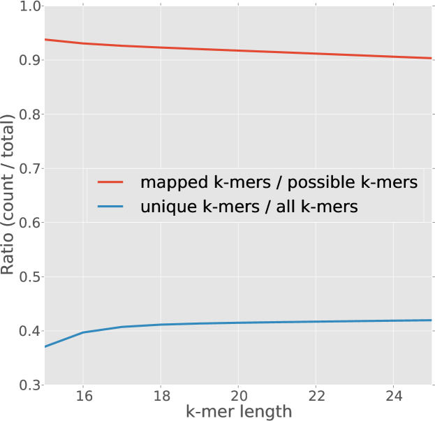
Supplementary Figure 1: As the k-mer length is varied in the range $[15,25]$ when processing the synthetic dataset, we observe that a longer k-mer length results in a slight decrease in data retention (denoted by the red line which shows the ratio of number of k-mers from the read set that were hashable to the total number of k-mers appearing in the set of reads). Simultaneously, we observe that the ratio of the number of unique k-mers (k-mers having a unique locus of origin) in the set of transcripts to the total number of k-mers in the set of transcripts (blue line) increases as we make $k$ larger. It seems that, as expected, there is a trade-off in the choice of $k$, with a larger $k$ resulting in less robustness to sequencing error but a higher fraction unique k-mers and smaller k-mers providing more robustness to errors in the data but at the cost of increased ambiguity. However, since the differences are relatively small over a reasonably large range of $k$, we can expect the inference procedure to be fairly robust to this parameter. We use $k=20$ for all experiments, and this is the default in Sailfish. However, we did not attempt to optimize this parameter when performing our experiments.

Supplementary Figure 2: Speed of counting indexed k-mers

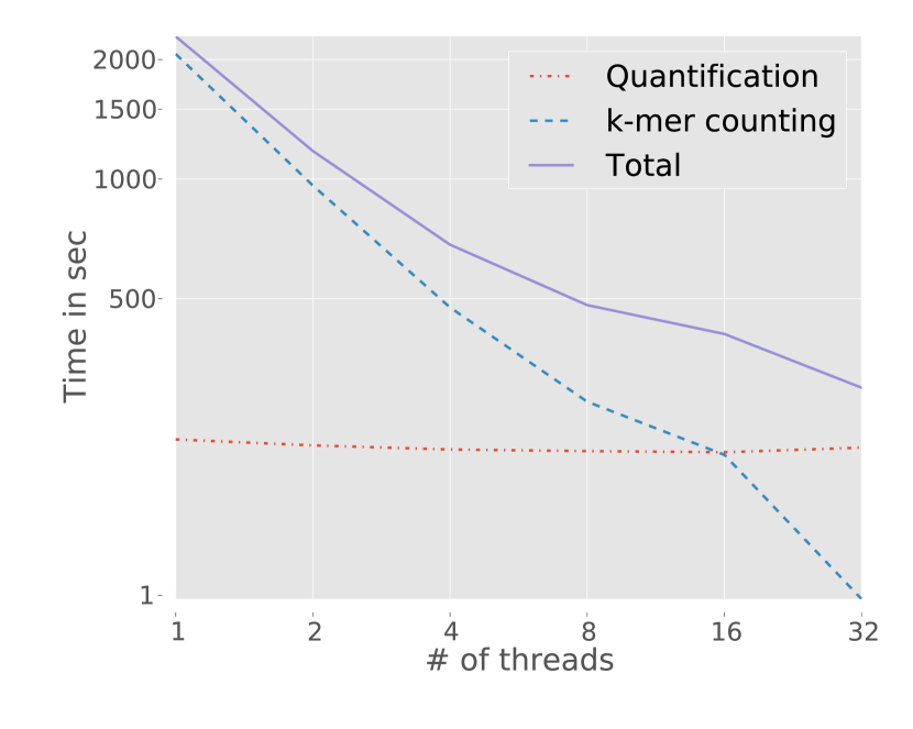
Supplementary Figure 2: The time to count all of the k-mers and quantify transcript abundance in an $81$M read dataset (SRX016366) as function of the number of concurrent hashing threads. Even with only a single thread, the counts for all k-mers in the dataset can be processed in $34$ minutes and $26$ seconds, while with $32$ processing threads, all k-mers can be counted in only $1$ minute and $28$ seconds.

Supplementary Note 1: Additional benefits of the Sailfish approach

An additional benefit of our lightweight approach is that the size of the indexing and counting structures required by Sailfish are a small fraction of the size of the indexing and alignment files required by most other methods. For example, for the MAQC dataset described in Figure LABEL:fig:results, the total size of the indexing and count files required by Sailfish for quantification was 2.4Gb, compared with much larger indexes and accompanying alignment files in BAM format used by other approaches (e.g., the 15.5Gb index and alignment file produced by Bowtie [4]). Unlike alignment files which grow with the number of reads, the Sailfish index files grow only with the number of unique k-mers and the complexity of the transcriptome’s k-mer composition and are independent of the number of reads.

Supplementary Figure 3: Correlation plots with qPCR on human brain tissue and synthetic data

RSEM	eXpress	Cufflinks

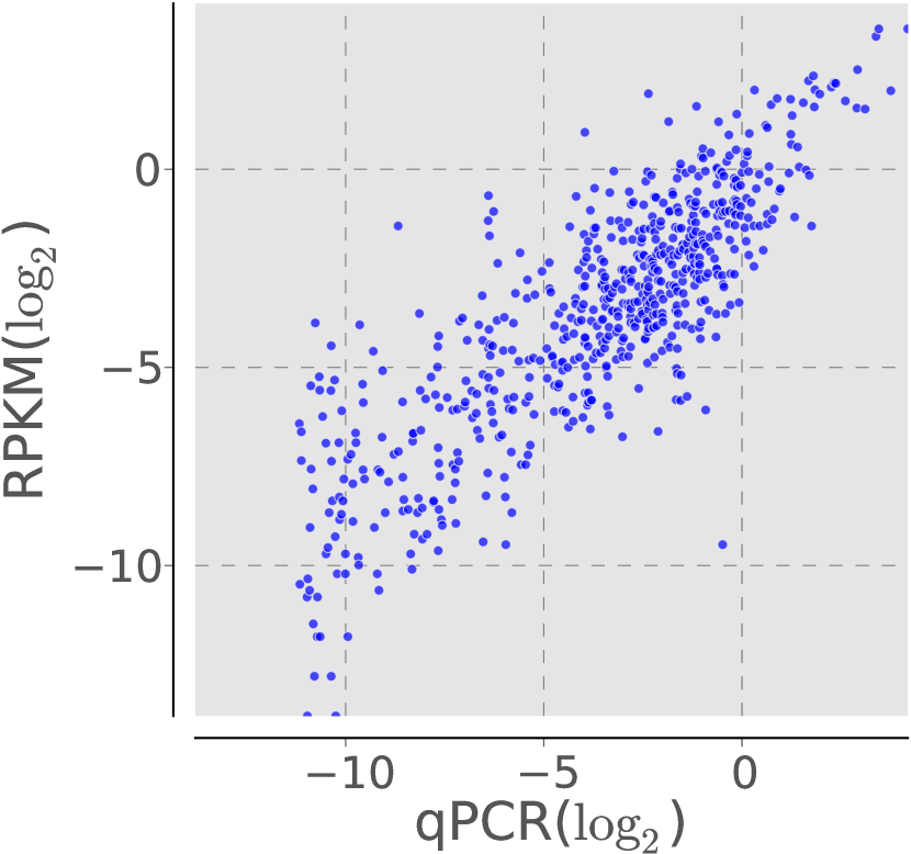
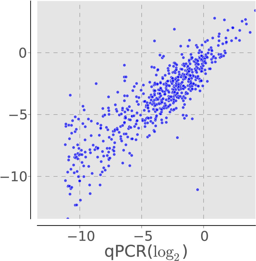
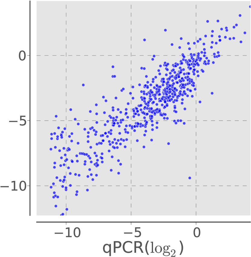
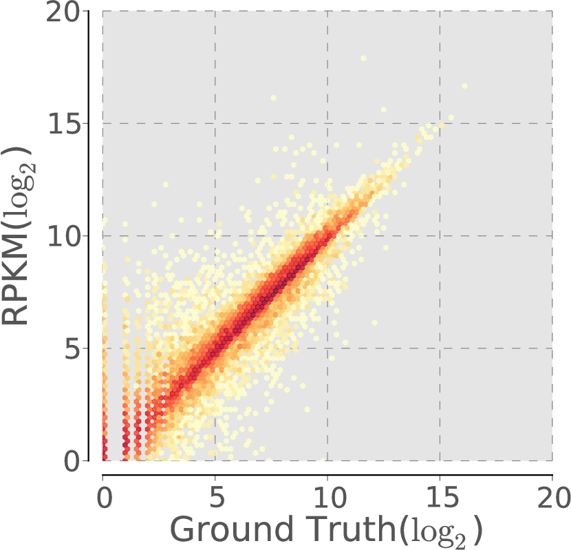
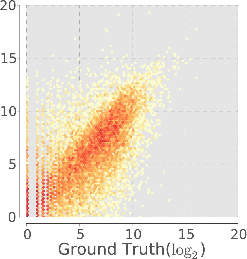
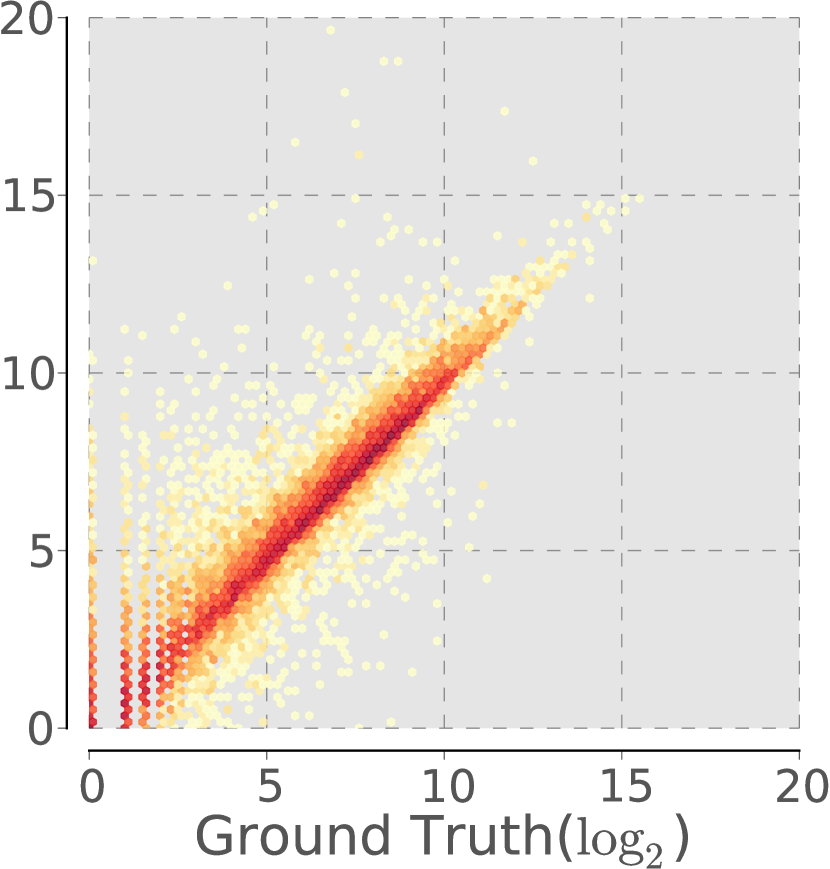
Supplementary Figure 3: Correlation plots of RSEM, eXpress and Cufflinks for the data presented in Fig. LABEL:fig:results. Each column is labeled with the method whose output was used to produce that column’s plots. The top row of plots show the correlation between the computed RPKM and the qPCR-based expression estimates for the human brain tissue. The bottom row of plots shows the correlation between the computed RPKM and the true abundance of each transcript on the synthetic dataset. To generate the results shown here, eXpress was run using its default streaming expression estimation algorithm. As reported in Methods, additional batch EM iterations improve eXpress’s accuracy, but come at the cost of a substantial increase in runtime.

Supplementary Figure 4: Correlation with qPCR on universal human reference tissue

Sailfish	RSEM	eXpress	Cufflinks

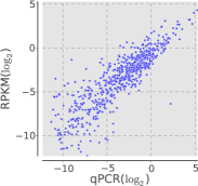
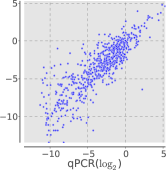
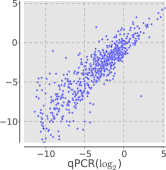
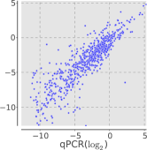
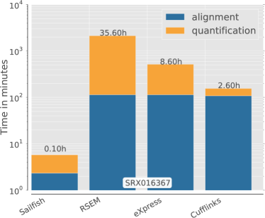
	Sailfish	RSEM	eXpress	Cufflinks
Pearson	0.87	0.85	0.87	0.87
Spearman	0.88	0.85	0.88	0.88
RMSE	1.64	1.81	1.65	1.68
medPE	29.95	34.77	31.03	27.33

Supplementary Figure 4: The accuracy of four methods on a second dataset from the MACQ [12] study. The reads for this experiment were taken from SRA accession SRX016367 ($\approx 93$M reads) and are from a mixture of different tissues (i.e. the Universal Human Reference or UHR). The same set of reference transcripts were used as in Fig. LABEL:fig:results of the main text. The relative accuracy and performance of the methods is similar to what we observed in the other MACQ dataset, with Sailfish, eXpress and Cufflinks all achieving comparable accuracy (all slightly more accurate than RSEM). Sailfish is $\approx 26$ times faster then Cufflinks, the closest method in terms of speed.

Supplementary Note 2: Additional details of accuracy analysis

We compare predicted abundances using correlation coefficients (Pearson & Spearman), root-mean-square error (RMSE), and median percentage error (medPE). These metrics allow us to gauge the accuracy of methods from different perspectives . For example, the Pearson correlation coefficient measures how well trends in the true data are captured by the methods, but, because the correlation is taken in the log scale, it discounts transcripts with zero (or very low) abundance in either sample, while the RMSE includes transcripts with true or estimated abundance of zero. Both eXpress and Cufflinks produced a few outlier transcripts, with very low but non-zero estimated abundance, which significantly degraded the Pearson correlation measure. We discarded these outliers by filtering the output of these methods, and setting to zero any estimated RPKM less than or equal to 0.01, a cutoff chosen because it removed the outliers but did not seem to discard any other truly expressed transcripts.

Supplementary Note 3: Parameters for simulated data

The simulated RNA-seq data was generated by the FluxSimulator [3] v1.2 with the following parameters.

### Expression ###
NB_MOLECULES    5000000
REF_FILE_NAME   hg19_annotations.gtf
GEN_DIR         hg19/chrs
LOAD_NONCODING  NO
TSS_MEAN        50
POLYA_SCALE     NaN
POLYA_SHAPE     NaN
### Fragmentation ###
FRAG_SUBSTRATE  RNA
FRAG_METHOD     UR
FRAG_UR_ETA     350
FRAG_UR_D0      1
### Reverse Transcription ###
RTRANSCRIPTION  YES
RT_PRIMER       RH
RT_LOSSLESS     YES
RT_MIN  500
RT_MAX  5500
### Amplification ###
GC_MEAN NaN
PCR_PROBABILITY 0.05
FILTERING       NO
### Sequencing ###
READ_NUMBER     150000000
READ_LENGTH     76
PAIRED_END      YES
ERR_FILE        76
FASTA           YES
UNIQUE_IDS      YES

Supplementary Figure 5: Convergence of relative abundance estimates

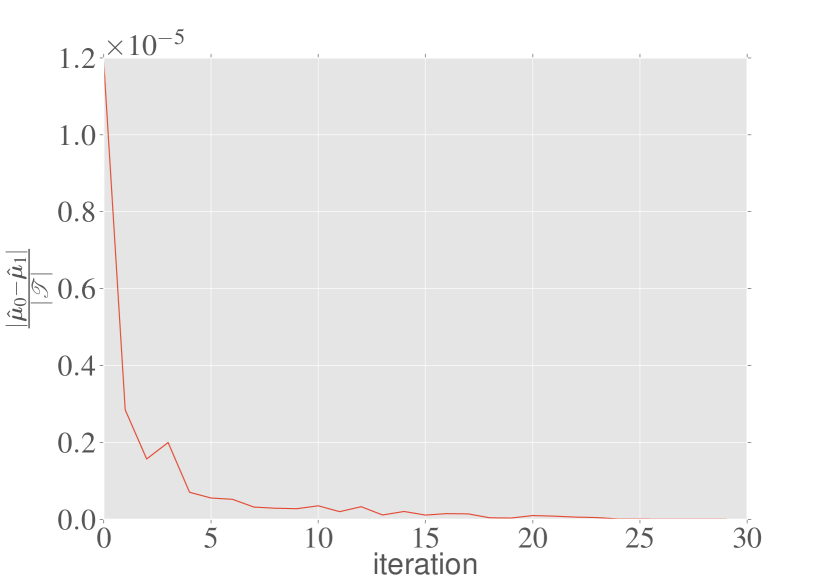
Supplementary Figure 5: The average difference between the relative abundance as estimated by two successive applications of the EM step (Algo. 2 lines 1–2) versus iterations of the SQUAREM algorithm (in the Universal Human Reference tissue experiment). We can see that the residual drops off quickly, and appears to have converged before 30 iterations of the SQUAREM procedure have been performed.

References

- [1] F. C. Botelho, R. Pagh, and N. Ziviani. Simple and space-efficient minimal perfect hash functions. In Algorithms and Data Structures, pages 139–150. Springer, 2007.
- [2] P. Flicek, I. Ahmed, M. R. Amode, D. Barrell, K. Beal, S. Brent, D. Carvalho-Silva, P. Clapham, G. Coates, S. Fairley, et al. Ensembl 2013. Nucleic Acids Research, 41(D1):D48–D55, 2013.
- [3] T. Griebel, B. Zacher, P. Ribeca, E. Raineri, V. Lacroix, R. Guigó, and M. Sammeth. Modelling and simulating generic RNA-Seq experiments with the flux simulator. Nucleic Acids Research, 40(20):10073–10083, 2012.
- [4] B. Langmead, C. Trapnell, M. Pop, S. L. Salzberg, et al. Ultrafast and memory-efficient alignment of short DNA sequences to the human genome. Genome Biology, 10(3):R25, 2009.
- [5] B. Li and C. Dewey. RSEM: accurate transcript quantification from RNA-Seq data with or without a reference genome. BMC Bioinformatics, 12(1):323, 2011.
- [6] G. Marçais and C. Kingsford. A fast, lock-free approach for efficient parallel counting of occurrences of k-mers. Bioinformatics, 27(6):764–770, 2011.
- [7] A. Mortazavi, B. A. Williams, K. McCue, L. Schaeffer, and B. Wold. Mapping and quantifying mammalian transcriptomes by RNA-Seq. Nature Methods, 5(7):621–628, 2008.
- [8] C. Pheatt. Intel threading building blocks. Journal of Computing Sciences in Colleges, 23(4):298–298, Apr. 2008.
- [9] K. D. Pruitt, T. Tatusova, G. R. Brown, and D. R. Maglott. NCBI Reference Sequences (RefSeq): current status, new features and genome annotation policy. Nucleic Acids Research, 40(D1):D130–D135, 2012.
- [10] A. Roberts, L. Pachter, et al. Streaming fragment assignment for real-time analysis of sequencing experiments. Nature methods, 10(1):71–73, 2013.
- [11] S. Roychowdhury, M. K. Iyer, D. R. Robinson, R. J. Lonigro, Y.-M. Wu, X. Cao, S. Kalyana-Sundaram, L. Sam, O. A. Balbin, M. J. Quist, T. Barrette, J. Everett, J. Siddiqui, L. P. Kunju, N. Navone, J. C. Araujo, P. Troncoso, C. J. Logothetis, J. W. Innis, D. C. Smith, C. D. Lao, S. Y. Kim, J. S. Roberts, S. B. Gruber, K. J. Pienta, M. Talpaz, and A. M. Chinnaiyan. Personalized oncology through integrative high-throughput sequencing: A pilot study. Science Translational Medicine, 3(111):111ra121, 2011.
- [12] L. Shi, L. H. Reid, W. D. Jones, R. Shippy, J. A. Warrington, S. C. Baker, P. J. Collins, F. De Longueville, E. S. Kawasaki, K. Y. Lee, et al. The MicroArray Quality Control (MAQC) project shows inter-and intraplatform reproducibility of gene expression measurements. Nature Biotechnology, 24(9):1151–1161, 2006.
- [13] C. Soneson and M. Delorenzi. A comparison of methods for differential expression analysis of RNA-seq data. BMC Bioinformatics, 14(1):91, 2013.
- [14] C. Trapnell, L. Pachter, and S. L. Salzberg. TopHat: discovering splice junctions with RNA-Seq. Bioinformatics, 25(9):1105–1111, 2009.
- [15] C. Trapnell, B. A. Williams, G. Pertea, A. Mortazavi, G. Kwan, M. J. van Baren, S. L. Salzberg, B. J. Wold, and L. Pachter. Transcript assembly and quantification by RNA-Seq reveals unannotated transcripts and isoform switching during cell differentiation. Nature Biotechnology, 28(5):511–515, 2010.
- [16] R. Varadhan and C. Roland. Simple and globally convergent methods for accelerating the convergence of any EM algorithm. Scandinavian Journal of Statistics, 35(2):335–353, 2008.
- [17] G. P. Wagner, K. Kin, and V. J. Lynch. Measurement of mRNA abundance using RNA-seq data: RPKM measure is inconsistent among samples. Theory in Biosciences, 131(4):281–285, 2012.
- [18] W. Zheng, L. M. Chung, and H. Zhao. Bias detection and correction in RNA-Sequencing data. BMC Bioinformatics, 12(1):290, 2011.