Interpreting Cross-correlations of One-bit Filtered Seismic Noise
keywords:
Theoretical Seismology – Wave scattering and diffraction – Wave propagation.Seismic noise, generated by oceanic microseisms and other sources, illuminates the crust in a manner different from tectonic sources, and therefore provides independent information. The primary measurable is the two-point cross-correlation, evaluated using traces recorded at a pair of seismometers over a finite-time interval. However, raw seismic traces contain intermittent large-amplitude perturbations arising from tectonic activity and instrumental errors, which may corrupt the estimated cross-correlations of microseismic fluctuations. In order to diminish the impact of these perturbations, the recorded traces are filtered using the nonlinear one-bit digitizer, which replaces the measurement by its sign. Previous theory shows that for stationary Gaussian-distributed seismic noise fluctuations one-bit and raw correlation functions are related by a simple invertible transformation. Here we extend this to show that the simple correspondence between these two correlation techniques remains valid for non-stationary Gaussian and a very broad range of non-Gaussian processes as well. For a limited range of stationary and non-stationary Gaussian fluctuations, we find that one-bit filtering performs at least as well as spectral whitening. We therefore recommend using one-bit filtering when processing terrestrial seismic noise, with the substantial benefit that the measurements are fully compatible with current theoretical interpretation (e.g., adjoint theory). Given that seismic records are non-stationary and comprise small-amplitude fluctuations and intermittent, large-amplitude tectonic/other perturbations, we outline an algorithm to accurately retrieve the correlation function of the small-amplitude signals.
1 Introduction
The study of terrestrial seismic noise correlations holds great promise as a means of generating new crustal constraints and studying its temporal variations (e.g., Brenguier et al., 2007; Wegler & Sens-Schonfelder, 2007; Brenguier et al., 2008; Zaccarelli et al., 2011; Rivet et al., 2011). These low amplitude waves are excited by storms, oceanic wave microseisms and related mechanisms (e.g., Longuet-Higgins, 1950; Nawa et al., 1998; Kedar & Webb, 2005; Stehly et al., 2006) at a variety of frequencies. Because these sources are typically not co-spatial with tectonically active regions, waves thus created illuminate the crust differently. Further, these types of seismic sources constantly excite wave noise, implying a continuous ability to monitor the crust.
A widely used technique in the processing of continuous seismic noise measurements (discovered by Weichert, 1904) consists of applying a digitizing one-bit filtering, introduced to the field first by Aki (1965). The method is straightforward, involving replacing the raw measurement by its sign (after removing secular variations), certainly a very useful technique in ca. 1965 when computer memory was highly limited (which is why it was used; private communication, G. Ekström 2012; also see Derode et al., 1999; Larose et al., 2004; Gerstoft & Tanimoto, 2007). Cupillard et al. (2011) also studied this problem and derived a relationship which connects the raw cross-correlation to the one-bit correlation. However Cupillard et al. (2011) make some incorrect assumptions in their analysis, leading them to a result that differs from those of van Vleck & Middleton (1966) and others.
The method has gained traction over subsequent decades and is used very widely in seismic noise analysis today. The primary benefits attributed to one-bit digitized over raw processing are the superior stability of correlation measurements. Observers who actively deal with such measurements undoubtedly ‘know’ (for instance, Derode et al., 1999; Larose et al., 2004) that finite-time estimates of correlation functions obtained from sufficiently long one-bit digitized signals tend to provide accurate and robust approximations of ‘true’ correlations. Here, we approach this problem more systematically and shed some light on the reasons behind the success of this method in seismological applications. Throughout this work, we assume that the ‘true’ signal arises from noise sources with well behaved statistics, i.e., we consider these sources with a bounded variance. In such a setting, we first discuss desirable properties of one-bit and other non-linear modulators in the idealized infinite-time case. In particular, we show that the normalized one-bit and raw correlation functions are approximately related by a simple trigonometric transformation; this relationship is exact for a Gaussian seismic noise and a wide class of non-Gaussian perturbations. Insight into the finite-time artifacts and advantages of the one-bit correlation techniques are studied subsequently by corrupting the synthetic small-amplitude seismic noise traces with intermittent large-amplitude (tectonic) spikes.
We show in the following sections that one-bit clipping of the measured seismic signals works extremely well in diminishing the impact of intermittent large-amplitude events especially when estimating the correlations from a finite-time sample. Further, it is believed that the one-bit correlation is a better approximation of Green’s function between the stations (e.g., Larose et al., 2004). However, we show here that it is merely a better measurement of the noise cross-correlation when these large spikes are present in the traces (note that Green’s function and cross-correlations are in general different, e.g., Hanasoge, 2013).
The study of correlations of digitized stochastic Gaussian-distributed processes has a long history, stretching back almost 80 years. In particular, we draw from two articles, van Vleck & Middleton (1966) and Hall (1969), in which the former calculate the correlation function of digitized Gaussian processes while the latter estimate the signal-to-noise degradation incurred due to the application of the one-bit filter. In the field of seismology, it was discussed by e.g., Tomoda (1956); Aki (1957), but is not used in contemporary noise tomography and its properties have not been carefully investigated for relevant problems.
We reproduce some aspects of that calculation in the context of a digitized bivariate Gaussian process; this is done first within a simple Gaussian framework and, subsequently, as a particular case for non-Gaussian statistics. These results are then validated and illustrated on the 2-D models developed in Hanasoge (2013). We study configurations of stationary and non-stationary sources to characterize the performance of the one-bit correlation. Finally, we examine the impact of ‘earthquake’ type perturbations on the estimated correlations of the seismic noise. In all cases, we find that the one-bit correlation method performs at least as well as when correlating raw measurements, and is markedly superior (i.e., in that it is closer to the ‘true’ noise correlation) when ‘earthquakes’ are present. In the appendix, we consider the generalized framework for computing the correlation functions of the output for a large family of non-linear filters applied to a range of non-Gaussian stochastic processes.
2 Statistics of Southern-California noise measurements
The underpinning of the theoretical arguments we lay out here is the assumption that seismic noise fluctuations are Gaussian random processes. To demonstrate that this is a valid assumption, we study measurements of vertical seismic velocity taken by station ‘ADO’, operated by California Institute of Technology, in the tectonically active region of southern California. We use 68 hours of measurements, taken during Jan 1-3 2010, which are frequency-filtered in the ranges 5-10 and 10-20 seconds. From this time series, we construct a histogram of the fluctuations and normalize it to obtain the empirical probability density function (pdf) of vertical seismic velocity. The data and the pdf are plotted in Figure 1.
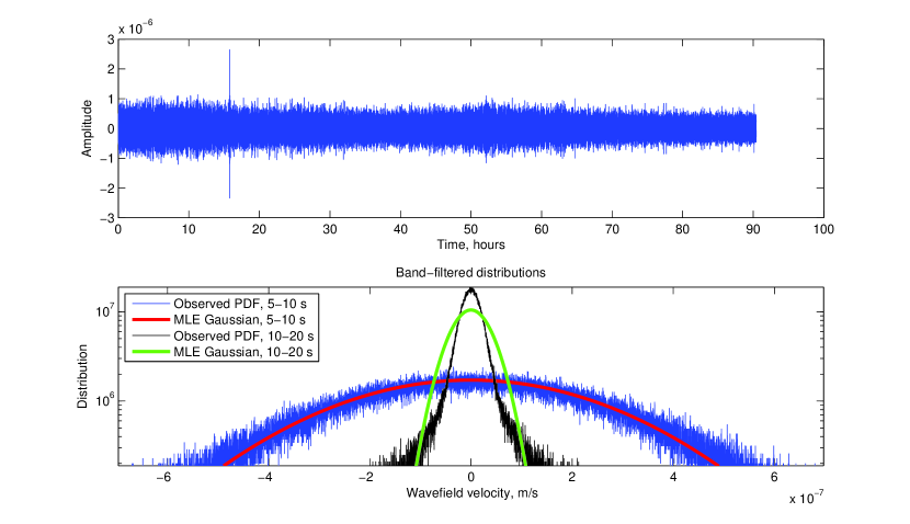
Assuming the data are Gaussian-distributed, we perform a maximum-likelihood fit (shown in red, lower panel). We compare the two pdfs using the Kullback-Leibler (K-L) divergence, which is an information-theoretic measure of the distance between a pair of pdfs. In the discrete case, the K-L divergence is given by,
| (1) |
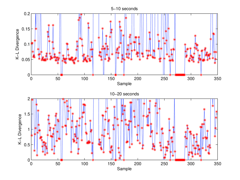
where is the empirical (observed) pdf and is the fit. We choose a Gaussian model for to perform the fit. The smaller the value of the K-L divergence, the better the information contained in a process with pdf is captured by the model ; the K-L divergence is zero only when . Figure 1 shows empirical pdfs and corresponding maximum-likelihood fits associated with 5-10 and 10-20 second bands for a 68-hour sequence. In Figure 2, we choose 348 instances of 68-hour measurement windows, perform a maximum-likelihood fit a Gaussian pdf to each interval and measure the K-L divergence between the data and the fit. A non-zero K-L divergence indicates non-Gaussianty. In general, non-Gaussianity may take arbitrary forms, i.e., long tails, oscillations in the distribution around a Gaussian etc. and no metric can unambiguously quantify the nature of the departure from a Gaussian distribution (i.e., non-Gaussianity is a non-unique notion). One can therefore only compare K-L divergences to say that the 5-10 second band is much better fit by a Gaussian than the 10-20 second series (see Figures 1 and 2). A much more detailed picture of the distribution and stationarity characteristics of seismic fluctuations may be found in Groos & Ritter (2009). Ultimately, neither Gaussianity nor stationarity are necessary for one-bit processing since we have developed a theory to address seismic fluctuations drawn from a broad range of distributions.
3 One-bit correlation
Guided by the preceding section, we model seismic noise in the 5-10 second bands as a multivariate Gaussian random process. Consider two stationary correlated zero-mean random sequences and , which represent seismic noise displacements measured at stations 1 and 2. We are interested in the connection between one-bit-digitzed and raw cross-correlations between these two sequences. The one-bit filter behaves as a non-linear Signum or sign function of the raw signal, mapping analogue signals, defined on the set of real numbers, to a digital :
| (2) |
The finite-time estimate of the cross-correlation function of zero-centered seismic noise fluctuations recorded at two stations, , denoted by , is defined as
| (3) |
where is the temporal length of averaging and is time. We note that the normalized finite-time correlation function is related to the cross-correlation through
| (4) |
where the finite-time variance estimates of and are defined analogously as
| (5) |
If the processes are ergodic and have bounded non-degenerate covariance (which we implicitly assume throughout) the cross-correlation and the correlation function are given, respectively, by
| (6) |
where denotes the statistical ensemble average and the existence of the limits follows from the ergodicity assumption. In practice, the length of the averaging time interval must be at least several source correlation times or inter-station wave travel times (whichever is larger). If the noise fluctuations were an ergodic random process with bounded variance, it follows that the finite-time estimate of the cross-correlation function in (3) approaches the true cross-correlation in (6a) as the temporal window of averaging grows.
The primary goal of this section is to elucidate the link between the (infinite-time) cross-correlation of the input in (6) to the cross-correlation of the output of the one bit digitizer given by
| (7) |
with the normalized correlation function defined analogously to (6b) and denoted by . An elegant derivation of the link between the correlation function of the true Gaussian signal and the output of the one-bit filter was given in van Vleck & Middleton (1966); we briefly recapitulate it below in a suitable ‘bivariate’ formulation since this classical results has not been discussed in noise tomography applications. An alternative derivation of this result in a much more general framework is presented in Appendix B.1. Measurements at two stations may be treated as a bivariate Gaussian process, with correlation matrix ,
| (8) | |||||
where and is the determinant of the matrix. The correlation function of the two random variables given their joint pdf is defined as
| (9) |
Thus we have,
| (10) |
and upon defining and , the integral reduces to
| (11) |
Comparing with equation (4), we note that the left side of equation (11) is . The correlation function of one-bit filtered random variables is therefore given by
| (12) |
This integral may be evaluated in closed form
| (13) |
where
| (14) |
Using the identity that the total integral of the probability density function is 1, i.e.,
| (15) |
we may rewrite the split in equation (13) as
| (16) |
We introduce the transform , allowing us to rewrite the integral as
| (17) |
where the integral in (17) may be evaluated using the following identity
| (18) |
Consequently, the correlation functions may be written as
| (19) |
where the integral above may be evaluated using the well-known formula
| (20) |
The transfer function between one bit to raw correlations is given by
| (21) |
or, conversely,
| (22) |
Thus, for two stationary Gaussian processes there exists a simple one-to-one mapping (22) between the correlation function obtained from the raw data and the digitized one-bit correlation function ; see Appendix B.1 for a derivation of analogous result in a much more general framework. In what follows, we assume that the relationship (22) holds approximately for the finite-time estimates, and , of the normalized raw data and one-bit cross-correlation functions, i.e.,
| (23) |
We omit here the technical justification of the above assumption for brevity; intuitively, this can be seen by noticing that for two stationary ergodic processes, and , with finite means and variances the finite-time estimates of the correlation functions are Gaussian random variables with respective means given by and variances bounded by and for any in (3).
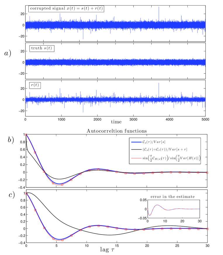
A few remarks are in order here. First, the relationship (22) is strictly valid for stationary Gaussian signals; a more general formula which does not require stationarity is derived in Appendix B.1 (see (63)). Second, the both the exact formula in (22) and its finite-time approximation (23) assume that the seismic noise signal is not corrupted by other sources. However, in the remainder of this paper we show that the recovery of the estimates of the correlation function from the one-bit digitized signal via (23) provides superior results to those obtained from finite time estimates, , obtained directly from the raw data. This is illustrated using both the numerical experiments and analytical results discussed in Appendix B.4 where we show that the relationship between the correlation function of the one-bit digitized signal and the correlation function of the Gaussian seismic noise is given, to a very good approximation, by the simple trigonometric formula (23) established in the Gaussian context. Remarkably, for a large class of bivariate non-Gaussian processes corrupting the accuracy of (23) is insensitive to the correlations between the corrupting processes, as also shown in Appendix B.4.
3.1 The transfer function and signal-to-noise ratio
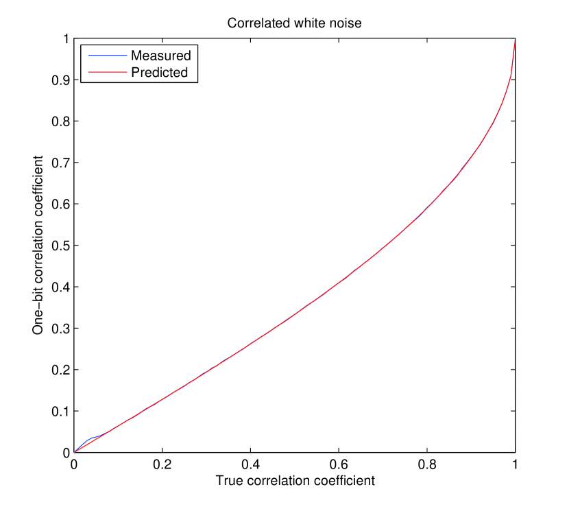
To numerically confirm equation (23), we generate sequences of delta-correlated random variables, i.e., where the correlation coefficient away from zero time-lag is statistically zero. This implies that there is only one characteristic correlation coefficient. It therefore allows us to easily test the accuracy of the transfer function (23), by comparing the one-bit-filtered and true correlation coefficients in Figure 3.
Because the digitizing filter results in the loss of phase information, the one bit output is noisier than the raw correlations. Evidently, the degradation in signal-to-noise ratio is dependent on a variety of factors, most importantly the specific definition of SNR and related issues such as the amount of noise present in the traces.
3.2 Band-limited Gaussian Random variables
Relation (23) provides us with a measurement algorithm:
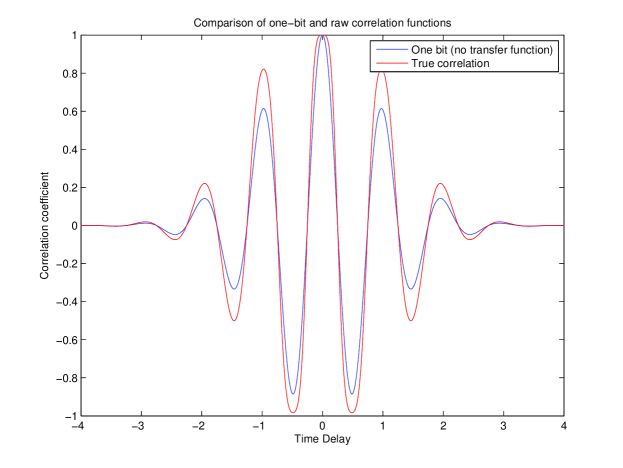
Terrestrial seismic noise is temporally band limited (owing, in large part, to instrumental limitations) and so it is natural to study this case next. In Figure 4, we show an artificially generated one-bit correlation function, i.e., , (blue) and the ‘true’ correlation function, which is defined by transfer function (22), i.e., . It is seen that the functions are similar but to improve the precision and accuracy of the measurement, it is necessary to apply relation (22). Unless specified explicitly, the output of this algorithm, i.e., where we have applied transfer function (23), will be termed ‘One-bit correlation’ in subsequent analyses and figures.
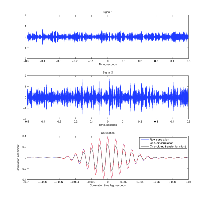
We confirm the statistical equivalence of one-bit and raw correlations of a stationary band-limited bivariate Gaussian random variable in Figure 5. Correlations, raw and one bit, of a large number of realizations of band-limited random variables are averaged to obtain estimates of the expectation value. It is seen that the agreement between the two is excellent (having applied the transfer function (23) on the correlation of the one-bit filtered traces).
In appendix B, we extend the results to stationary random variables drawn from a broad range of distributions. Gaussianity is therefore not a necessary condition for the oscillations. We also invoke stationarity, a central assumption in this analysis, one that is not generally representative of measurements. For non-stationary oscillations, the theory becomes much more complicated since the meaning of the “true” cross-correlation is not clear. For a stationary random variable with bounded variance, the one-bit correlation with transfer function has the same expectation value as the raw correlation.
Similar to this work, Cupillard et al. (2011) developed a theory of one-bit filtering based on concepts of “coherent” and “incoherent” noise, using it to characterize the functional relationship between one-bit and raw correlations. Their formalism requires knowing the coherent and incoherent constituents a priori, which may be very difficult to obtain. In contrast, with no knowledge of the coherence or the lack thereof, we provide an algorithm to estimate the true correlation coefficient given the one-bit measurement.
The main result of Cupillard et al. (2011), expressed in their equation (52), which connects the raw cross-correlation to the coherent and incoherent parts of the one-bit correlation, is slightly erroneous. In their appendix C, Cupillard et al. (2011) calculate the probability of the correlation of the two one-bit filtered traces assuming they are independent, which is in error. This leads them to a result that differs from those of van Vleck & Middleton (1966) and others.
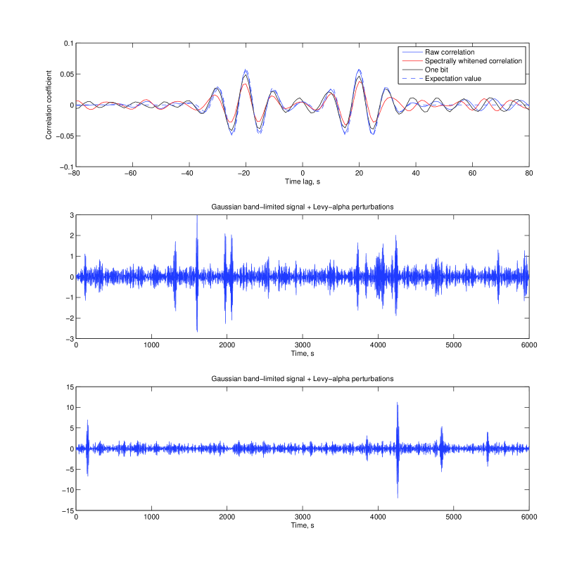
In Figure 6, we compare the method of spectral whitening to one-bit and raw correlations. Spectral whitening allows for a number of free parameters and our intention is not to explore the full regime; we assume the form (24), which is a variant of the method discussed by Seats et al. (2012). We compute the correlation of a stationary band-limited Gaussian random signal with a few transient perturbations drawn from a Lévy power-law distribution. The 6000-second signal in Figure 6 is divided into segments of 200 seconds each, auto-correlations are computed for each segment normalized by its power spectrum. These 30 correlations are averaged and multiplied by the average power spectrum of the segments. In other words, the spectrally whitened correlation function is computed so
| (24) |
where original signals and are divided into segments and , and with each segment multiplied by a window function to set it smoothly to zero at the edges. The average power spectrum of the processes are denoted by and . The raw and one-bit correlations are accurate and closely match the expected value but the spectrally whitened correlation shows slightly larger errors in amplitude and phase. Even in the case when there are no transient perturbations, i.e., where the signal is purely Gaussian, spectral whitening converges more slowly to the expected correlation amplitude than one-bit and raw correlations. Indeed, we do not perform an exhaustive parametric study, and it may be that in some regimes, spectral whitening does better. We also note that, most importantly, there is a theoretical basis for interpreting the one-bit correlations and that with transfer function (23), we recover the expectation value of the correlation function.
The question of what happens when the distribution of seismic noise fluctuations is non-Gaussian is indeed valid. In appendix B, we discuss more generalized distributions (i.e., non-Gaussian fluctuations) and address a range of non-linear modulators. For the cases we have studied, where the fluctuations possessed exponential/ other heavy-tailed distributions, we find that relation (23) still remains very effective.
3.3 Non-stationary processes
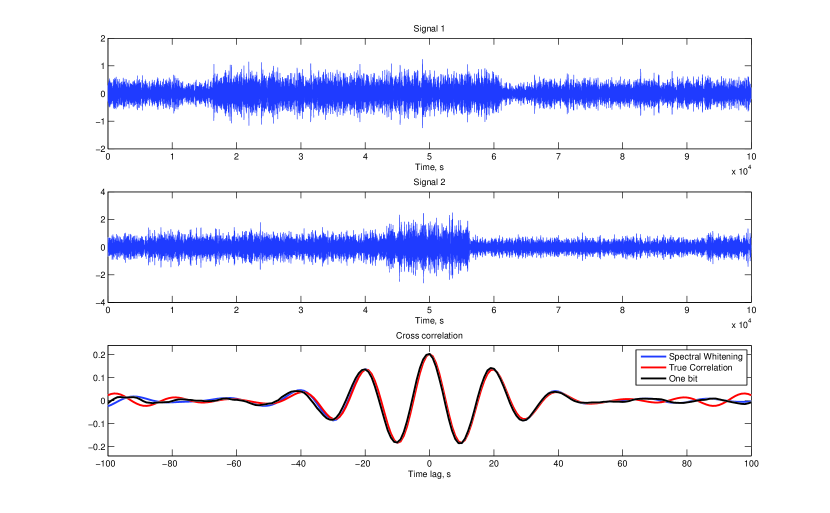
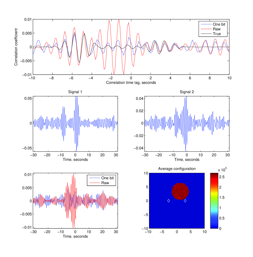
We characterize the performance of spectral whitening and one-bit filtering applied to statistically non-stationary processes, a common feature of observed seismic fluctuations. We generate sequences of stationary bivariate Gaussian signals and their correlation function is termed the ‘true’ correlation function. These processes are subsequently modulated in time so as to generate a process whose variance changes, and thus is temporally non-stationary. From this test, we find in Figure 7 that correlations derived from one-bit filtering are essentially identical to those obtained by spectral whitening.
4 Demonstration using the wave equation
Here we study wave propagation in a 2-D homogeneous background, where wave excitation is effected by a temporally stochastic and spatially non-uniform distribution of sources. The goal is to simulate wave noise, record this at a pair of stations and cross correlate them over many realizations (or long periods of time; we assume ergodicity here). Raw and one-bit filtered noise traces are correlated and compared to the (‘true’) expectation value.
The relation (38) when applied to equation (3) gives us the cross-correlation function in the Fourier domain
| (25) |
where the are random variables and is the Fourier transform of the finite-time estimate of the cross-correlation. Were it to exist, the limit (or expected) cross-correlation, denoted by , is
| (26) |
Note that is a random variable whereas is a fixed quantity.
For the sake of simplicity, we consider wave propagation in a 2-D plane, described by
| (27) |
where is density, is a 2-D flat space, time, the wave displacement, the covariant spatial derivative, the source and wavespeed. We also assume a constant wavespeed . Green’s function for the displacement due to a spatio-temporal delta source at is the solution to
| (28) |
Green’s function in the Fourier domain for this wave equation is given by
| (29) |
where is temporal frequency and is the Hankel function of the first kind. To reduce notational burden, we assume an implicit frequency dependence in all terms (unless otherwise specified). Thus the wavefield excited by sources is described by
| (30) |
Thus by treating is a complex random variable, we may artificially generate temporal sequences of seismic noise with very little computational cost. Upon computing these displacement traces, we investigate the properties of cross-correlations subject to generalized source distributions and signal processing methods. The correlation in Fourier domain (25) may be rewritten in terms of Green’s functions and sources
| (31) |
If the variance of the complex random variable were to be bounded, the expectation value of the cross-correlation (26) exists and is given by
| (32) |
For the demonstrations here, we assume that sources at all spatial points are described by independent and identically distributed random variables, resulting in spatial decoherence, i.e.,
| (33) |
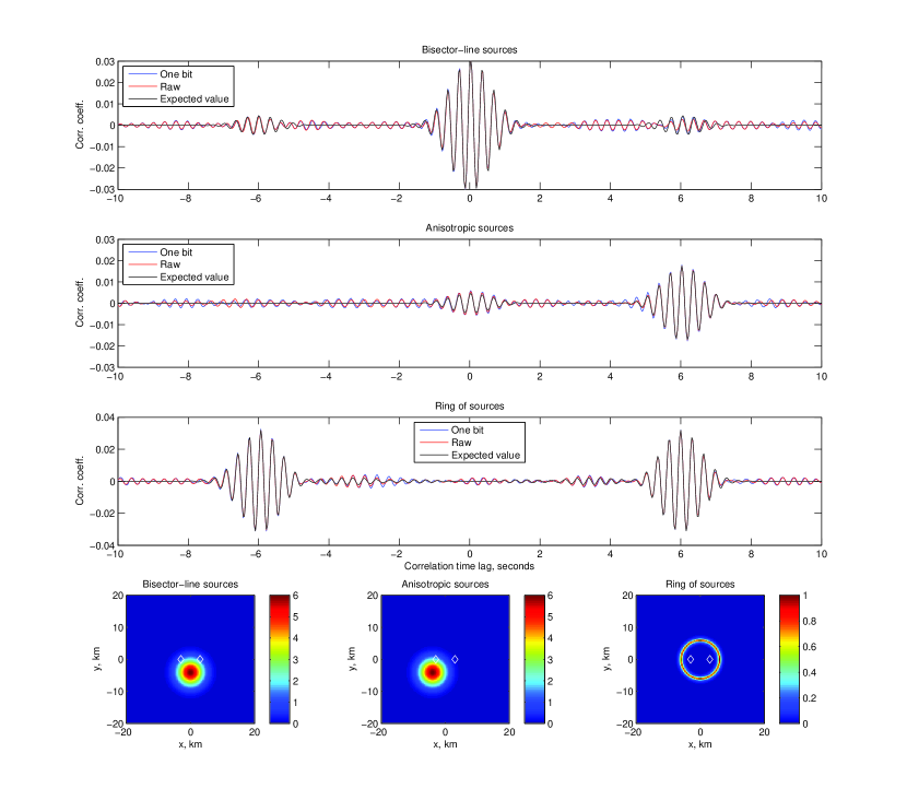
In order to generate realizations of seismic traces, we populate the source function with sequences of independent and identically distributed random variables . The seismic displacements at a given station is simply the product of Green’s function between the source location and the realization . In this manner, one can investigate the impact of different statistical distributions of sources on one-bit and raw cross-correlations. In Figure 8, we consider a pair of stations illuminated by two spatially non-uniform arrangements of sources, placed along the bisector line and off-axis in two cases. We create 12000 realizations of sources and each realization of seismic traces are raw and one-bit correlated. These correlations are then summed over all these realizations and the one-bit correlations are converted according to relation (23). The correlations in Figure 8 show that both one-bit and raw converge to the expectation value although they are both noisy.
To further test the method, we consider sources that spatially non-stationary Gaussian, with and without large-amplitude perturbations (‘earthquakes’). We draw realizations of the non-Gaussian perturbations from the heavy-tailed Lévy alpha-stable distribution.
4.1 Spatially inhomogeneous and non-stationary Gaussian sources
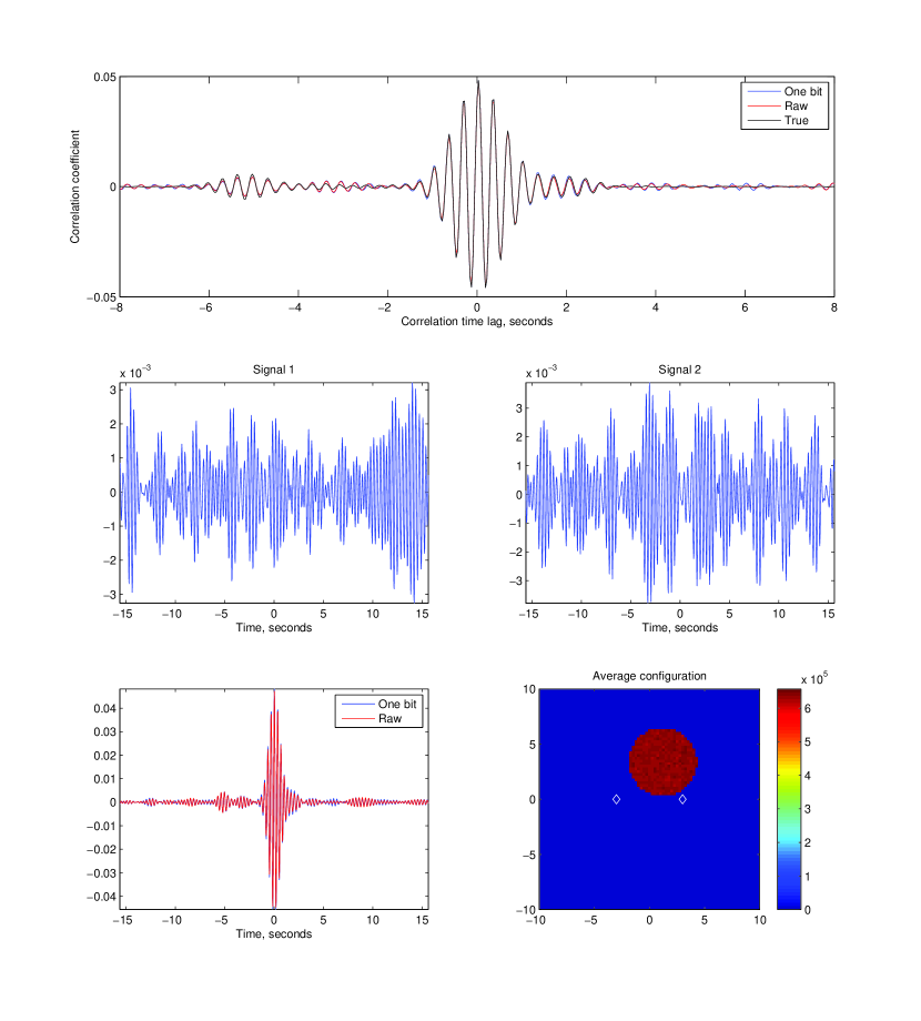
In this experiment, we perform 20000 realizations in which sources are assigned to a randomly chosen set of spatial locations. Each realization consists of a randomly chosen number of source points within the disc shaped region shown on the bottom-right panel of Figure 9. Thus the sources ‘jump around’ from one realization to the next. This is done to mimic a plausible scenario where sources both spatially and temporally stochastic. We assume as before that the sources are spatially incoherent, i.e., that they are spatially uncorrelated. For each source, we populate its frequency domain representation with complex Gaussian random variables and using Green’s theorem (30), generate seismic traces at the two stations. We average the spatial arrangements of sources over all the realizations to obtain the “average configuration” as shown in Figure 9. The expectation value of the cross-correlation is then computed using equation (32) and compared with the raw and one-bit filtered correlations. In order to make the comparison, we apply the transfer function (23). The agreement between the three curves is excellent.
4.2 ‘Earthquake’ perturbations
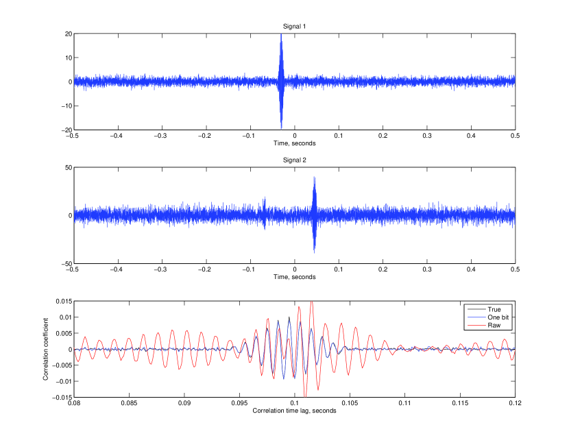
In this experiment, we generate band-limited realizations of bivariate Gaussian random variables. These are likened to noise-source generated seismic signals. We correlate these signals and term them the ‘true correlation’. Seismic records contain noise and earthquake related signals alike and consequently, in order to model the latter, we introduce intermittent large-amplitude transient oscillatory signals into the measurements. In the upper two panels of Figure 10, we show an example of a stochastic realization with a superposed ‘earthquake’. The amplitude of the earthquake measurements is chosen randomly from a Cauchy distribution, which belongs to the Lévy-alpha-stable family. Random variables from this family have unbounded variances and consequently, correlation functions of such stochastic process are non-existent. Raw- and one-bit correlations are computed and averaged over 8000 realizations, and we compare them to the true correlation in the lowest panel of Figure 10. One-bit and true correlations are much more similar to each other than the raw correlation, which is noisy and appears to be out of phase. Note that because the ‘earthquake’ amplitudes are Cauchy distributed, the raw correlation does not converge to an expectation value. In contrast, the one-bit correlation is well behaved, with the one-bit filter clipping the tail of the distribution and large-amplitude events are weighted to the same extent as noise. Consequently, the one-bit and true correlations are very similar.
5 Conclusions
We have studied and categorized the statistical properties of one-bit and raw correlations. Overall, our assessment is that the one-bit correlation is a more stable measurement, able to handle large-amplitude signals due to sporadic sources, with signal-to-noise characteristics superior in the presence of these perturbations and at worst, comparable to the raw correlation. A summary of the assumptions and properties of the method are listed
-
•
The theory applies to both stationary and non-stationary random processes, which obey either Gaussian or a broad range of other distributions (see appendix B),
-
•
If these assumptions are true, correlations obtained through one-bit processing (with the transfer function) accurately recover the correlation function,
-
•
Simple tests with non-stationary processes show that the ‘true’ correlation (associated with small-amplitude fluctuations) is well recovered,
-
•
The short-window spectral-whitening method (a variant of the method discussed by Seats et al., 2012) converges at a rate similar to that of one-bit correlations for the cases we consider here,
-
•
Information is lost when one-bit filtering is applied and the signal-to-noise ratio will consequently be lower than when computing correlations using raw data for purely Gaussian distributed fluctuations. However, when the raw data are punctuated by large-amplitude transient events, the one-bit filtered correlations converge to the correct expectation value,
- •
Although a more comprehensive study is needed to fully characterize the signal-to-noise losses and gains, our tests show that using the one-bit filter to process terrestrial seismic noise can be very beneficial. One may recover the true noise correlation by first estimating the one-bit correlation, applying transfer function (23), and multiplying the resultant by the standard deviations of the measurements at the two stations. This way, one can reconstruct the correct amplitudes of the cross correlations and this information is not lost. The elegance of using one-bit filtering lies in being able to effortlessly move between the filtered and real domains. This implies that theoretical developments in aid of interpreting noise correlation measurements (e.g., Tromp et al. (2010); Hanasoge (2013)) need no altering, and the data processing techniques that are currently widely in use are fully justifiable. We conclude with an algorithm to leverage these benefits:
-
•
Measure , of the noise records as best as possible (i.e., by ignoring large-amplitude spikes)
-
•
Convert real measurements at pairs of stations into digital signals (apply the one-bit filter)
-
•
Correlate these signals, and determine the one-bit correlation function
-
•
Use transfer function 23 to move between the filtered domain to the real domain (i.e., )
-
•
Renormalize using the product of the measured standard deviations to recover the cross-correlation, i.e.
- •
An important issue is whether the method of one-bit filtering remains effective when the distribution of seismic noise fluctuations is non-Gaussian. Does equation (23), which allows us to move so easily between the filtered and real domains, continue to remain valid? In appendix B, we have discussed more generalized distributions (i.e., non-Gaussian fluctuations) and address a range of non-linear modulators. For the cases we have studied, where the fluctuations possessed exponential/ other heavy-tailed distributions, we find that relation (23) still remains very effective.
Acknowledgements
S. M. H. is funded by NASA grant NNX11AB63G and thanks Courant Institute, New York University for its hospitality and Göran Ekström for useful conversations. We also warmly thank Cornelis Weemstra for his careful reading and considerable help in improving the manuscript and an anonymous referee for helping us tighten our narrative. This work is an effort to understand cross-correlations in helioseismology in the context of DFG CRC 963 Astrophysical Flow Instabilities and Turbulence .
References
- Aki (1957) Aki, K., 1957. Space and Time Spectra of Stationary Stochasic Waves, with Special Reference to Microtremors, Bulletin of the Earthquake Research Institute, 35, 415–457.
- Aki (1965) Aki, K., 1965. a Note on the Use of Microseisms in Determining the Shallow Structures of the Earth’s Crust, Geophysics, 30, 665.
- Brenguier et al. (2007) Brenguier, F., Shapiro, N. M., Campillo, M., Nercessian, A., & Ferrazzini, V., 2007. 3-D surface wave tomography of the Piton de la Fournaise volcano using seismic noise correlations, Geophys. Res. Lett., 34, 2305.
- Brenguier et al. (2008) Brenguier, F., Campillo, M., Hadziioannou, C., Shapiro, N., Nadeau, R., & Larose, E., 2008. Postseismic relaxation along the san andreas fault at parkfield from continuous seismological observations, Science, 321(5895), 1478–1481.
- Cupillard et al. (2011) Cupillard, P., Stehly, L., & Romanowicz, B., 2011. The one-bit noise correlation: a theory based on the concepts of coherent and incoherent noise, Geophysical Journal International, 184, 1397–1414.
- Derode et al. (1999) Derode, A., Tourin, A., & Fink, M., 1999. Ultrasonic pulse compression with one-bit time reversal through multiple scattering, Journal of Applied Physics, 85(9), 6343–6353.
- Gerstoft & Tanimoto (2007) Gerstoft, P. & Tanimoto, T., 2007. A year of microseisms in southern California, Geophys. Res. Lett., 34, 20304.
- Groos & Ritter (2009) Groos, J. & Ritter, J., 2009. Time domain classification and quantification of seismic noise in an urban environment, Geophysical Journal International, 179(2), 1213–1231.
- Gumbel (1960) Gumbel, E. J., 1960. Bivariate exponential distribution, Journal of the American Statistical Association, 56, 698–707.
- Hall (1969) Hall, H. M., 1969. Power spectrum of hard-limited Gaussian processes, The Bell System Technical Journal, pp. 3031–3057.
- Hanasoge (2013) Hanasoge, S. M., 2013. The influence of noise sources on cross-correlation amplitudes, Geophysical Journal International, 192(doi: 10.1093/gji/ggs015), 295–309.
- Kedar & Webb (2005) Kedar, S. & Webb, F. H., 2005. The ocean’s seismic hum, Science, 307, 682–683.
- Larose et al. (2004) Larose, E., Derode, A., Campillo, M., & Fink, M., 2004. Imaging from one-bit correlations of wideband diffuse wave fields, Journal of Applied Physics, 95(12), 8393–8400.
- Longuet-Higgins (1950) Longuet-Higgins, M. S., 1950. A Theory of the Origin of Microseisms, Royal Society of London Philosophical Transactions Series A, 243, 1–35.
- Middleton (1948) Middleton, D., 1948. Some general results in the theory of noise through non-linear devices, Quarterly of Applied Mathematics, 5, 445.
- Nawa et al. (1998) Nawa, K., Suda, N., Fukao, Y., Sato, T., Aoyama, Y., & Shibuya, K., 1998. Incessant excitation of the Earth’s free oscillations, Earth, Planets, and Space, 50, 3–8.
- Rice (1944) Rice, S. O., 1944. Mathematical analysis of random noise, Bell System Technical Journal, 24, 46–156.
- Rivet et al. (2011) Rivet, D., Campillo, M., Shapiro, N. M., Cruz-Atienza, V., Radiguet, M., Cotte, N., & Kostoglodov, V., 2011. Seismic evidence of nonlinear crustal deformation during a large slow slip event in Mexico, Geophys. Res. Lett., 38, 8308.
- Seats et al. (2012) Seats, K. J., Lawrence, J. E., & Prieto, G. A., 2012. Improved ambient noise correlation functions using Welch’s method, Geophysical Journal International, 188(2), 513–523.
- Stehly et al. (2006) Stehly, L., Campillo, M., & Shapiro, N. M., 2006. A study of the seismic noise from its long-range correlation properties, Journal of Geophysical Research, 111(B10306).
- Tomoda (1956) Tomoda, Y., 1956. A Simple Method for Calculating the Correlation Coefficient, Journal of Physics of the Earth, 4, 67–70.
- Tromp et al. (2010) Tromp, J., Luo, Y., Hanasoge, S., & Peter, D., 2010. Noise cross-correlation sensitivity kernels, Geophysical Journal International, 183, 791–819.
- van Vleck & Middleton (1966) van Vleck, J. H. & Middleton, D., 1966. The spectrum of clipped noise, Proceedings of the IEEE, 54(1), 2–19.
- Wegler & Sens-Schonfelder (2007) Wegler, U. & Sens-Schonfelder, C., 2007. Fault zone monitoring with passive image interferometry, Geophysical Journal International, 168(3), 1029–1033.
- Weichert (1904) Weichert, E., 1904. Verhandlungen der Zweiten Internationalen Seismologischen Konferenz, in Gerlands Beitrag Geophysik, pp. 41–43, Leipzig, Germany.
- Zaccarelli et al. (2011) Zaccarelli, L., Shapiro, N. M., Faenza, L., Soldati, G., & Michelini, A., 2011. Variations of crustal elastic properties during the 2009 L’Aquila earthquake inferred from cross-correlations of ambient seismic noise, Geophys. Res. Lett., 38, 24304.
Appendix A Fourier Convention
We apply the Fourier convention below
| (34) | |||||
| (35) | |||||
| (36) | |||||
| (37) |
where are a Fourier transform pair. Cross-correlations and convolutions in the Fourier and temporal domain are described by
| (38) |
| (39) |
For real functions , we also have
| (40) |
Appendix B General framework for assessing the statistical properties of nonlinear modulators
The goal here is to obtain general formulas linking the the cross-correlation function
for two signals, measured at different stations, to the cross-correlation function of modulated signals
is a nonlinear modulator with known characteristics. We seek an exact or approximate link allowing to recover from . This framework is much more general than the one outlined in the main text due to the following reasons:
-
•
No stationarity in the measured signals, and is assumed for the most part,
-
•
The measured signals, and are assumed to contain both the seismic noise component and some unwanted sources of tectonic origin, i.e., ; the assumption here that the processes have non-Gaussian statistics with fat tails indicative of intermittent events, e.g., events of tectonic origin.
-
•
A wide class of nonlinear modulators is discussed; the one-bit digitizer discussed in the main text is but one member of the class.
We seek an exact or approximate link allowing to recover the information about the seismic noise, , from the modulated correlation function of the modulated signal which is corrupted by the tectonic sources. Motivated by the earlier work in Rice (1944); Middleton (1948); Hall (1969), we express the correlation function of the modulated signal via an integral involving the characteristics of the modulator and the joint characteristic function of the input signals. Exact analytical or approximate formulas for can be derived if the joint characteristic function of the input signals can be represented as a series of appropriately factorized terms; such a factorized series representation is possible for a large class of Gaussian and non-Gaussian processes, as shown below. In particular, in §B.3 we provide an alternative derivation of the simple trigonometric link (23) between the Gaussian seismic noise correlations and its modulated correlations. We then show that for a large class of bivariate non-Gaussian processes the correlation function of the filtered corrupted signals is insensitive to the correlations between the corrupting processes and it is the same as for uncorrelated processes with . Most importantly, the relationship between the correlation function of the modulated signal and the correlation function of the Gaussian seismic noise is given, to a very good approximation, by the simple trigonometric formula (23) established in the Gaussian context.
B.1 General formula for the cross-correlation function
Here, we consider the statistics of the modulated signal given the known characteristics of the input signal and the characteristics of the modulator which we assume to have the Laplace transform representation
| (41) |
where and is a suitable contour in the complex plane. The main focus is on nonlinear modulators and it is well known that a large class of such devices can be represented in such a way (e.g., Rice (1944); Middleton (1948)). The key feature of the integral representation (41) is that the cross-correlation function of the modulated signals and can be expressed via an integral involving the joint characteristic function of the input as
| (42) |
where is the joint density associated with the input pair ; here and below, we skip the explicit dependence on in the joint density in order to simplify the notation. Note that the last integral in (B.1) is the joint characteristic function of given by
| (43) |
so that we can express the cross-correlation of the modulated signal (B.1) through the Laplace transform of the filter and the joint characteristic function of the input signal as
| (44) |
The attractive property of the exact formula in (44) is that it splits the properties of the modulator, represented by the terms involving , from the properties of the input signal encoded in the characteristic function .
Here, we assume that the input signals and contain the signal of interest and perturbations; our goal is to examine the ability of the modulator to recover the statistical properties of the signal from the input which is corrupted by some unwanted processes ; thus, we write the input signal as
| (45) |
where the perturbations are independent of . Given the form of the input as in (45), its joint characteristic function factorizes as
| (46) |
B.2 Special cases of the general framework
The utility of the general framework described above becomes apparent when the joint characteristic functions of the truth signal and of the corrupting process can be factorized as
| (47) |
so that
| (48) |
Given the factorization in (B.2), the autocorrelation of the modulated signal (44) becomes
| (49) |
where
| (50) | |||
| (51) |
The form of and in (49) depends on the modulator and the statistics of the input signal. A particular class of modulators commonly used in signal processing analyzed is introduced below.
B.2.1 The family of nonlinear modulators
We consider a one parameter class of nonlinear modulators described by
| (52) |
where the constant parameterizes the family. The filter in (52) has the following integral representation (cf. (41))
| (53) |
where we exploit the Laplace transform of with the contours given, respectively, by
| (54) |
and the transforms, , are expressed through the Gamma function, , as follows:
| (55) |
The two-parameter family of modulators in (52) contains a large class of modulators ranging from a trivial linear case to the one-bit modulator the properties of which are the main focus here.
B.3 Cross-correlation functions for one-bit filtered Gaussian processes
Here, we show that in the particular case of uncorrupted Gaussian signal, , modulated by the so-called ideal limiter , the correlation functions of the input and of the modulated output are related by
| (56) |
where . This result obtained by reducing the general non-Gaussian framework of §B.1-B.2.1 is complementary to the derivation discussed in section 3 which requires the Gaussianity assumptions from the outset. Consider a ‘canonical’ Gaussian process with autocorrelation and the joint characteristic function given by
| (57) |
where the second equality is due to the expansion
| (58) |
Consequently, the correlation function (49) of the digitized signal is given by
| (59) |
where
| (60) |
The contour integrals in (60) above can be evaluated in a standard fashion noticing (we skip details here) that in such a case both contours can be shifted to the imaginary line so that upon substituting in (60), we obtain
| (61) |
and the autocorrelation function (59) becomes
| (62) |
Further simplifications in (62) can be achieved using the fact that
for any integer which leads to
| (63) |
If the signals are stationary, i.e., for all , the above expression simplifies to
| (64) |
as claimed at the beginning of this section.
B.4 Cross-correlation functions for a signal consisting of Gaussian and non-Gaussian components
Here, we consider non-Gaussian perturbations to the seismic noise signals measured at two different stations. We show that for a large class of densities the correlation function of the filtered corrupted signals is insensitive to the correlations between the corrupting processes and the same as for uncorrelated processes with . Most importantly the relationship between the correlation function of the filtered corrupted signal and the correlation function of the Gaussian seismic noise is given, to a very good approximation, by the simple trigonometric formula (56).
Consider the two input signals, to consist of the Gaussian components corrupted by processes with Cauchy-like density (at any fixed time)
| (65) |
It is well known (e.g., Gumbel (1960)) that construction of joint probability density of a bivariate process with given marginal densities, which is necessary for deriving the characteristic function in (43), is non-unique. One possible way of constructing such a joint density with arbitrary correlation function is via the following formula
| (66) |
where are odd functions and chosen such that . Below we show that for this class of densities the correlation function of the corrupted signals is insensitive to the correlations between the corrupting processes and the same as for the delta-correlated process , i.e., .
Consider, in particular, the following two-point density with the structure as in (66)
| (67) |
where is the cross-correlation of and and the marginal cumulative distribution function is given by
| (68) |
and the normalization constant in (67) is .
The joint characteristic function for the Gaussian signal has the same form as in (57) and the joint characteristic function of the perturbing processes is given in the factorized form as
| (69) |
the Fourier transforms in (69) have no analytical expressions and are computed numerically below. Consequently, the correlation function of the modulated input signal signal is given by
| (70) | |||
| (71) |
where
| (72) | ||||
| (73) |
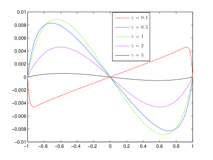
The contour integrals in (72)-(73) above can be evaluated in a standard fashion using (53) and (55), and noticing (we skip details here) that in such a case both contours can be shifted to the imaginary line ; thus, upon substituting (55) for and in (72), (73), we obtain
| (74) |
and
| (75) |
The result in (75) is due to the fact that is an odd function. Consequently, the correlation function in (59) simplifies to
| (76) |
which is independent of the cross-correlation of the processes . Note, however, that the coefficients in (79) are functions of the variances of the two processes; thus, the mapping induced by (79) depends on the variances, , of the corrupting processes . However, it turns out that for the ideal limiter (i.e, with ) the dependence on in (79) can be approximately factored out as follows (see figure 12)
| (77) |
so that the unwanted dependence on when estimating from (77) can be removed by the following normalization
| (78) |
the high accuracy of this approximation is illustrated in figure 12. Additional illustration of the high accuracy of the estimation of the correlation function from the corrupted input is shown in figure 13 where, for simplicity, both processes are assumed identical and stationary so that the correlation of the modulated signal (77) reduces to
| (79) |
