Astrophysically robust systematics removal using variational inference: application to the first month of Kepler data

Abstract

Space-based transit search missions such as Kepler are collecting large numbers of stellar light curves of unprecedented photometric precision and time coverage. However, before this scientific goldmine can be exploited fully, the data must be cleaned of instrumental artefacts. We present a new method to correct common-mode systematics in large ensembles of very high precision light curves. It is based on a Bayesian linear basis model and uses shrinkage priors for robustness, variational inference for speed, and a de-noising step based on empirical mode decomposition to prevent the introduction of spurious noise into the corrected light curves. After demonstrating the performance of our method on a synthetic dataset, we apply it to the first month of Kepler data. We compare the results, which are publicly available, to the output of the Kepler pipeline’s pre-search data conditioning, and show that the two generally give similar results, but the light curves corrected using our approach have lower scatter, on average, on both long and short timescales. We finish by discussing some limitations of our method and outlining some avenues for further development. The trend-corrected data produced by our approach are publicly available.

1 Introduction

Surveys for planetary transits monitor tens or hundreds of thousands of stars at high precision, with rapid time sampling, and over long periods. The resulting datasets can be used not only to discover and characterise transiting exoplanets, but also to study a wide range of phenomena of stellar origin, such as pulsations, rotation, and binarity. However, transit survey data are typically affected by a wide range of artefacts, many of which affect all the target stars simultaneously, although to varying degrees.

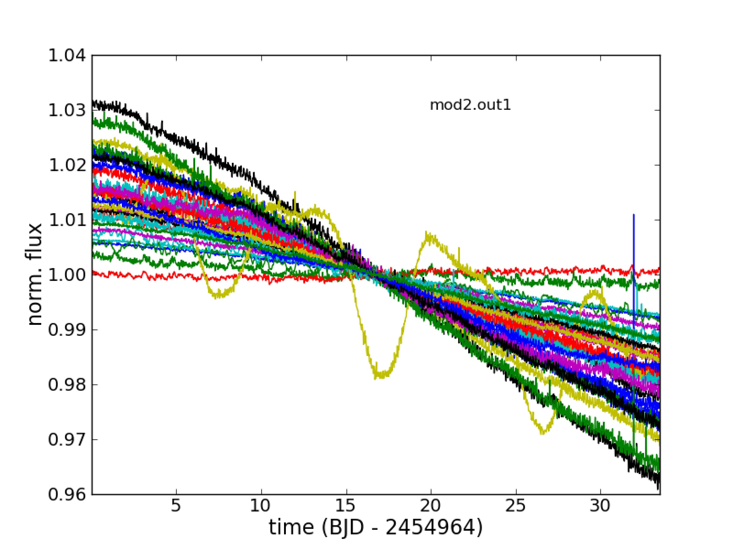
The Kepler space mission, launched on March 6, 2009 (Borucki et al., 2010), exemplifies this opportunity and the associated challenges. The unprecedented precision and baseline of the $\sim$150 000 Kepler light curves, most of which are now in the public domain, opens up the possibility of studying the micro-variability of stars other than the Sun for the first time, probing amplitudes ranging from a few parts per thousand to a few parts per million, and timescales of weeks to years. However, there are also artefacts in the raw data, particularly long term trends, which are prominent in the light curves of all but the highest variability stars. This is visible in Figure 1, which shows a set of example light curves from the first month of Kepler observations, known as Quarter 1 (hereafter Q1; see Section 3.2 for more details).

These common-mode instrumental effects are usually known as systematics. When the cause of the systematics is understood well enough, it is possible to formulate explicit models for their removal. In many other situations, however, we have little knowledge regarding the nature or number of systematic trends in the data. In this paper we present the development of a new methodology, which we refer to as Astrophysically Robust Correction (ARC), which addresses the issue of discovering and removing underlying systematics in astronomical data. We apply the method to data from the first quarter (Q1) of Kepler data, and show that it efficiently removes the systematic artefacts in that dataset. McQuillan, Aigrain, & Roberts (2012) used the resulting ’cleaned’ data to perform a preliminary statistical study of the variability of the Kepler target stars on month timescales.

Figure 1: Example raw light curves from Kepler quarter 1 data. The 30 light curves shown were selected at random among the 1290 objects observed in the first output channel on module 2 of the Kepler detector. Each light curve was normalised by dividing it by its median.

1.1 Existing methods

The problem of trend identification and removal in ensembles of stellar light curves was first addressed in the context of ground-based transit surveys, such as OGLE (Udalski et al., 2002), HatNET (Bakos et al., 2002), or SuperWASP (Pollacco et al., 2006). The sources of systematics in these surveys are atmospheric (e.g. differential airmass variations across the field-of-view, seeing and atmospheric transparency variations) as well as instrumental (e.g. pointing jitter combined with inter- and intra-pixel sensitivity variations). The two methods, which are most widely used to identify and remove systematics in ground-based transit surveys are known as SysRem (Tamuz, Mazeh, & Zucker, 2005) and TFA (Trend Filtering Algorithm, Kovács, Bakos, & Noyes 2005). SysRem attempts to explain each light curve as a linear superposition of all the other light curves, and adjusts the coefficients of this linear basis model so as to minimise the total squared variance of all the light curves. The resulting algorithm is very similar to Principal Component Analysis (PCA, see e.g. Wall et al. 2003), although it allows for individual weighting of each observation of each star. Because of this, the trends are not strictly orthogonal, and must be identified and removed iteratively. The number of times this is done must then represent a trade-off between removing systematics and preserving real variability. TFA proceeds in a similar fashion, but the trends are identified in a limited subset of the light curves, which is selected by the user, so as to contain a representative sample of the systematics, but minimal intrinsic variability.

The images from which the photometry is extracted, or ancillary sensors, can also be used to measure meteorological and instrumental parameters, which are thought to affect the photometry, for example seeing, airmass, detector temperature, etc…From these, one may construct a linear basis with which to model the systematics, a procedure known as external parameter decorrelation, (EPD, Bakos et al. 2007). EPD is usually applied as a preliminary step prior to running a search for additional trends using (e.g.) SysRem or TFA. Although the EPD method as described in Bakos et al. 2007 is designed for large ensembles of light curves, the same principle, namely fitting a given light curve with a linear combination of external parameters, can also be applied in situations where a single star is being monitored, for example high-precision observations of planetary transits or eclipses.

All three of the methods outlined above make a number of important assumptions:

• that the relationship between the trends and the light curves is linear;

• that the data used to identify the trends (light curves or external parameter data) is sufficient to describe them completely;

• that the majority of the stars are not significantly variable, so that systematics dominate the global sum of the squared residuals which is used as a figure of merit.

The third assumption becomes problematic in the case of space-based transit surveys such as Kepler and CoRoT (Baglin et al., 2009), which routinely reach sub-millimagnitude precision. As these missions are revealing, many, if not most, stars are intrinsically variable at that level. Intrinsic variability can become an important, if not dominant, contribution to the global figure of merit one is trying to optimize, exacerbating the problem of preserving this variability whilst removing the systematics. As a result, in PCA-like approaches, the first few principal components can easily be dominated by a small number of highly variable stars, which happen to account for a large fraction of the overall variance of the data. This problem is exacerbated by the fact that these methods are couched in the framework of maximum likelihood, and therefore are not robust against overfitting. Petigura & Marcy (2012) partially address this problem, by identifying and removing from the training set any light curves, whose basis coefficients are deemed anomalous. In this paper we go further, introducing a criterion which explicitly expresses our desiderata that the trends should be constituted of many small contributions from many light curves, and using a fully Bayesian model to avoid over-fitting (see Section 1.2).

The pipeline used to process Kepler data before releasing it to the public incorporates a ‘pre-search data conditioning’ (PDC) stage. The PDC is designed to remove instrumental systematics so as to optimize the efficiency of the transit detection process. Early implementations of the PDC (Jenkins et al., 2010) followed a procedure similar to EPD, but attempted to identify and remove signals of stellar origin in the frequency domain before applying the correction. This preserved astrophysical variability in some, but not all cases. Additionally, in some cases the PDC was found to introduce high-frequency noise into the light curves. This effect has been noted in a previous publication (Murphy, 2012) in which the noise properties of short (1-min) and long (30-min) cadence data were compared for the same targets. It is due to the fact that the estimate of each systematic trend is necessarily noisy. These issues made the PDC-processed light curves unsuitable for variability studies, and motivated the development of the alternative method, which is the subject of this paper. In the mean time, Kepler pipeline has also evolved. In more recent implementations of the PDC, known as PDC-MAP (maximum a-posteriori, Smith et al. 2012; Stumpe et al. 2012), a subset of highly correlated and quiet stars is used to generate a cotrending basis vector set, as well as a set of priors over the coefficients of each basis vector, which is then used in the correction of all the light curves. This leads to a significant improvement in robustness, but we shall defer a detailed comparison to Section 3.2.

1.2 Introducing the ARC

Our starting point in the development of a robust detection and correction methodology for the Kepler data was not fundamentally different to those of previously published methods: like virtually all of them, we use a linear basis model and identify the trends from the light curves themselves, as is done in SysRem and TFA. However, our approach differs in the following important ways:

• we perform the linear basis regression using the Variational Bayes (VB) method of approximate Bayesian inference to ensure that the procedure is robust to uncertainties in the data, while maintaining computational tractability and scalability to large datasets;

• we apply automatic relevance determination(ARD) priors to the coefficients of the basis vectors. These priors have zero mean and their individual widths are adjusted iteratively to maximise the model evidence. This ensures that trends are identified and removed only if there is significant evidence for them in the data;

• we formulate an explicit criterion, based on a measure of the entropy of each trend, to reflect our belief that the trends are systematic i.e. that they are present, at some level, in the majority of light curves, and that the contribution of any single light curve to any given trend should be small;

• we incorporate a de-noising step after the identification of each trend, which uses the empirical mode decomposition (EMD) algorithm, chosen to avoid any intrinsic bias towards trends on particular timescales.

The entropy criterion is similar in spirit to the modified PCA method of Petigura & Marcy (2012), but it actively selects trends which satisfy our desiderata, rather than merely rejecting problematic light curves.

This paper is structured as follows. Section 2 gives an overview of the ARC, focussing on aspects which are new and/or with which our intended readership may be unfamiliar, namely our trend selection and stopping criteria and the EMD algorithm. Section 3 shows some illustrative results, starting with a walk-through on a synthetic example dataset, and then moving on to the Kepler Q1 data. In Section 4, we compare the performance of the PDC-MAP and the ARC. Finally, Section 5 summarises the advantages and limitations of the ARC and discusses open questions on which future work will focus. Detailed descriptions of the Bayesian linear basis regression model and of the VB inference method are given for reference in Appendices A and B.

2 Method

The main challenge, when performing systematics removal with a linear basis model, is to identify the appropriate basis, i.e. the systematic trends. We adopt an iterative approach to this problem, isolating the most dominant systematic trend first, removing it and then repeating the process. At each iteration, the dominant systematic is identified by constructing a set of ‘candidate’ trends from the light curves themselves, ranking them according to the entropy criterion, selecting the top few candidates, combining them into a single time-series using PCA, and denoising the resulting trend. We now proceed to describe each of these steps in detail.

First, we introduce a few notation conventions. Our data consists of $N$ observations each of the relative flux of $M$ stars. Throughout this paper, we use the subscript $n(=1$, …, $N)$ to denote observation number and $m(=1$, …, $M)$ to denote the star number. We denote the $n^{\rm th}$ observation of star $m$ as $d_{nm}$, and the corresponding observation time $t_{n}$. The light curve of star $m$ forms a column vector $\mathbf{d}_{m}\equiv[d_{1m}$, …, $d_{Nm}]^{\sf T}$ (where $\mathbf{A}^{\sf T}$ is the matrix transpose of $\mathbf{A}$).

We consider each of the observed light curves, $\mathbf{d}_{m}$, to be composed of a linear combination of an underlying ‘true’ stellar signal, $\mathbf{s}_{m}$, an unknown number, $K$, of systematic trends, $\mathbf{u}_{k}$ ($k=1$, …, $K$), and an observation noise process, $\mbox{\boldmath$\epsilon$}_{m}$:

$$\mathbf{d}_{m}=\mathbf{s}_{m}+\sum_{k=1}^{K}a_{mk}\mathbf{u}_{k}+\mbox{\boldmath$\epsilon$}_{m}$$ (1)

where the unknown factors $a_{mk}$ represent the contribution of the $k^{\rm th}$ systematic trend to the $m^{\rm th}$ light curve.

Defining the ensemble of all other light curves, $\mathbf{D}_{m}=\{\mathbf{d}_{l\not=m}\}$, we seek to model as much of $\mathbf{d}_{m}$ as possible using $\mathbf{D}_{m}$ as a basis. This is achieved via a Bayesian linear model with inference performed using variational Bayes (see Appendices A and B for details) such that,

$$\mathbf{\hat{d}}_{m}=\sum_{l\not=m}w_{ml}\mathbf{d}_{l}$$ (2)

where the $\{w_{ml}\}$ are a set of weights. We repeat the process for each light curve in turn, resulting in a set of putative explanatory vectors $\{\mathbf{\hat{d}}_{m}\}$. In the remainder of this section, we refer to the $\mathbf{\hat{d}}_{m}$ as candidate trends, to distinguish them from the ‘adopted’ trends $\mathbf{u}_{k}$.

2.1 Trend entropy

Our primary hypothesis is that systematic trends are present in the majority of the light curves. Thus, if $\mathbf{\hat{d}}_{m}$ represents a linear combination of ‘true’ systematic trends, it should be composed of many small contributions from many of the other light curves, rather than a few dominant contributions from a small number of light curves. More formally, the distribution of the weights $\mathbf{w}_{m}=\{w_{ml}\}$ should have a high Shannon entropy (Shannon, 1951):

$$\mathcal{H}\left(\mathbf{w}_{m}\right)=-\sum_{l\not=m}p_{ml}\log_{2}p_{ml},$$ (3)

where we have defined

$$p_{ml}=\frac{w^{2}_{ml}}{\sum_{l^{\prime}\not=m}w^{2}_{ml^{\prime}}}$$ (4)

by analogy with a normalised probability distribution.

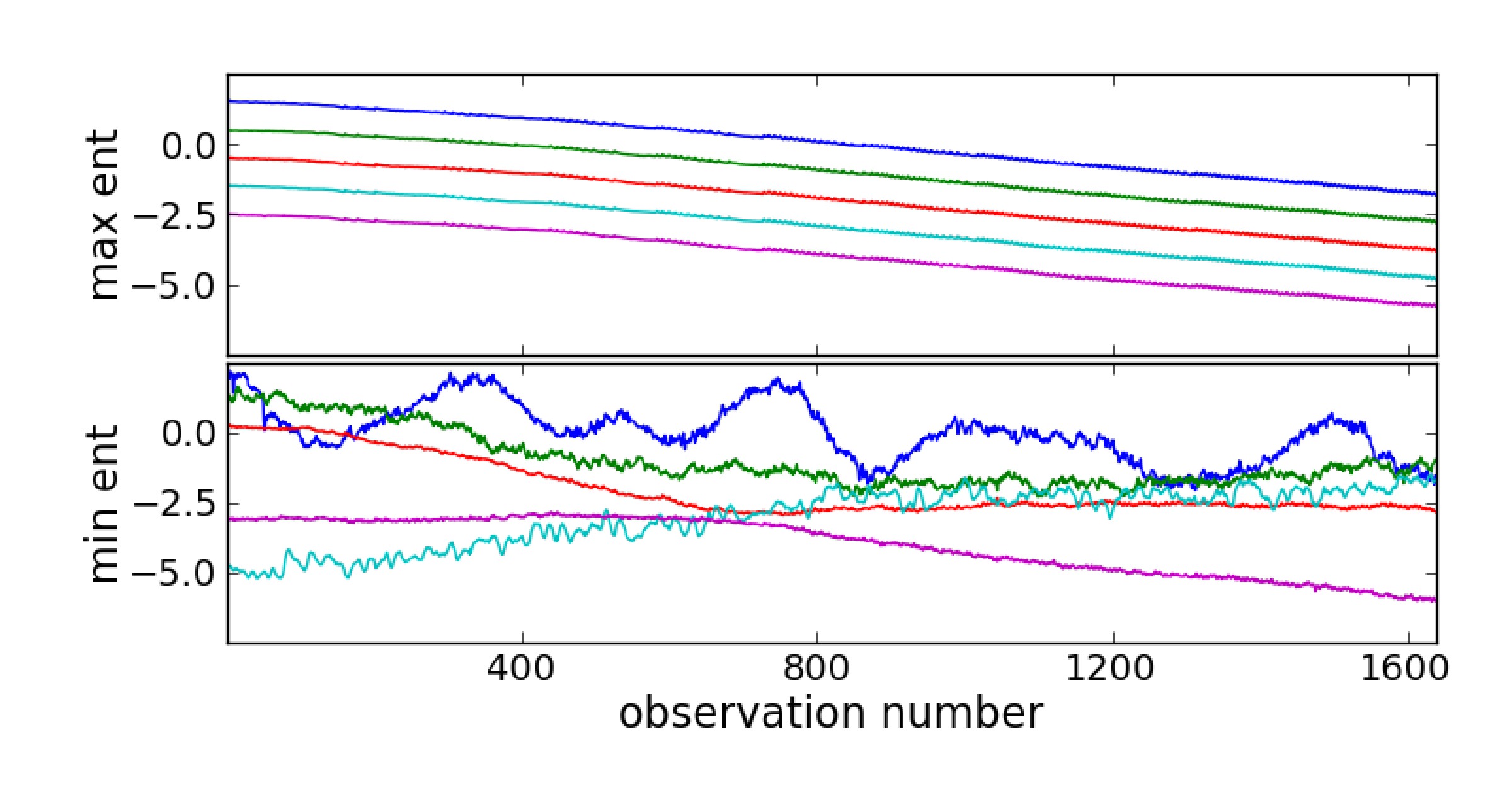
We therefore rank each candidate trend $\mathbf{\hat{d}}_{m}$ according to the entropy $\mathcal{H}\left(\mathbf{w}_{m}\right)$ of the associated set of weights. The $\mathbf{\hat{d}}_{m}$ with the highest entropy are expected to be mutually similar, since they all represent a systematic trend. On the other hand, those with the lowest entropy correspond to cases where a particular light curve was found to be very similar to one or two others, but not to the rest. This is illustrated in the case of the Kepler Q1 data by Figure 2. We form a reduced basis $\mathbf{T}$ by selecting the few candidate trends with the highest entropy. We normally use ten, but as the maximum entropy trends are mutually similar, the exact number (within reason) is not important.

Figure 2: Maximum (top) and minimum (bottom) entropy candidate trends for the Kepler Q1 data (using all of the Q1 light curves). The trends have been normalised to have zero mean and unit variance. Vertical offsets have been added and only five curves shown in each category to improve figure clarity.

2.2 Principal component analysis and spectral radius

If, as expected, the trends in the reduced basis $\mathbf{T}$ are representative of a single, dominant systematic, then they should be mutually similar, as illustrated in Figure 2. We can thus use PCA to extract a single trend from the reduced basis (the first principal component), and evaluate just how dominant this trend is. The first principal component of $\mathbf{T}$ contains most of the information, and explains most of the overall variance of $\mathbf{T}$.

We start by decomposing $\mathbf{T}$ into a pair of orthonormal matrices of singular components, $\mathbf{U}$, and $\mathbf{V}$, and a diagonal matrix $\mathbf{S}$ of singular values, $\sigma_{i}$. The latter are the square roots of $\lambda_{i}$, the eigenvalues of $\mathbf{TT}^{\sf T}$.

$$\mathbf{T}=\mathbf{USV}^{\sf T}.$$ (5)

$\mathbf{U}$ is also the matrix of eigenvectors of $\mathbf{TT}^{\sf T}$:

$$\mathbf{TT}^{\sf T}=\mathbf{U}\mathbf{S}\mathbf{S}^{\sf T}\mathbf{U}^{\sf T}=\mathbf{U}\mbox{\boldmath$\Lambda$}\mathbf{U}^{\sf T},$$ (6)

in which $\Lambda$ is a diagonal matrix of eigenvalues, $\{\lambda_{i}\}$. The spectral radius of each eigenvector, defined as

$$\rho_{i}=\frac{\lambda_{i}}{\sum_{j}\lambda_{j}},$$ (7)

is then a measure of the fraction of the overall variance of $\mathbf{T}$ explained by that eigenvector. In this paper we consider, in particular, the spectral radius,$\rho_{1}$, of the first eigenvector.

Figure 3: First principal component for the set of five maximum-entropy candidate trends shown in the top panel of Figure 2.

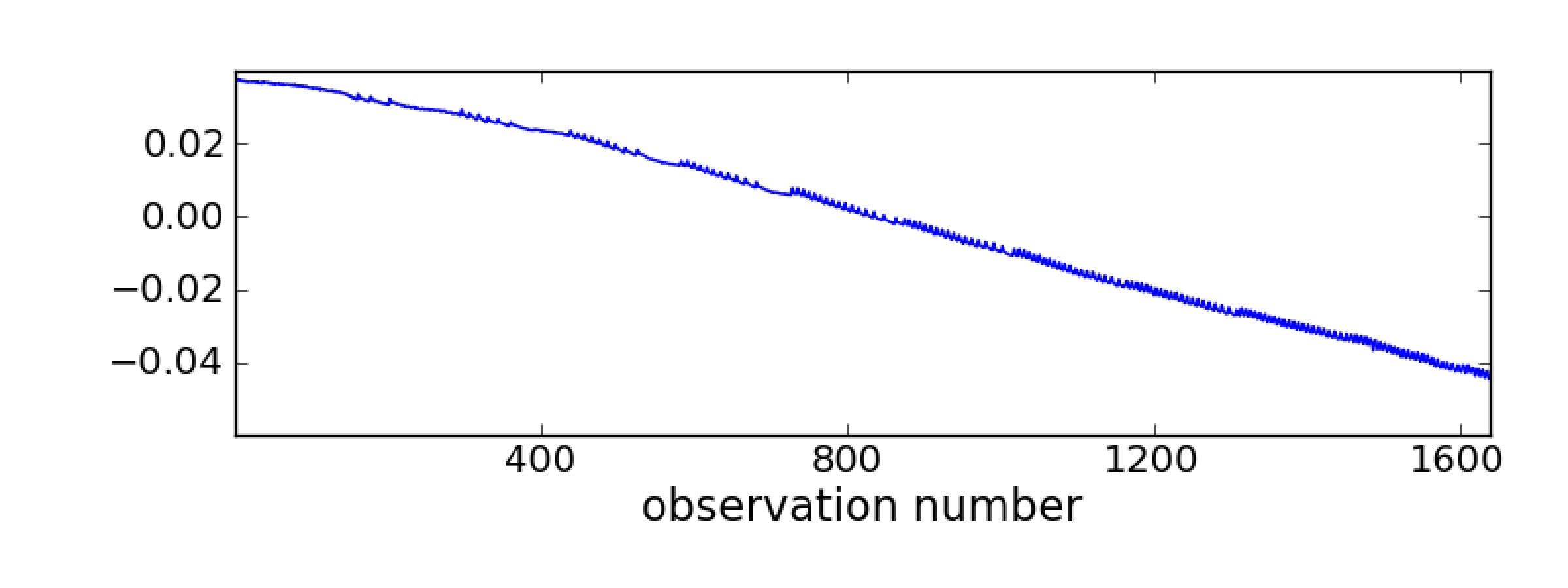
As discussed above, if the candidate trends which make up $\mathbf{T}$ are truly systematic, they should also be self-similar, and the spectral radius of the first principal component should be large (close to unity). If so, the first principal component contains pertinent information regarding the systematic trends in the data. For example, Fig. 3 shows the first principal component of the matrix $\mathbf{T}$ identified from all the Kepler Q1 light curves. Its spectral radius is $>0.99$, so it is highly representative of the $\mathbf{T}$, and it would be reasonable to adopt it as one of the $\mathbf{u}_{k}$. However, as it is a linear combination of a finite number of noisy light curves, it may still contain significant amounts of noise. Using it directly may therefore introduce noise into the light curves, particularly those of bright stars. Thus, we introduce a final de-noising step in our trend discovery process.

2.3 Empirical Mode Decomposition (EMD)

Empirical Mode Decomposition (EMD, Huang et al. 1998) decomposes a time-series into a series of intrinsic modes, each of which admits a well-behaved Hilbert transform, enabling the computation of an energy-frequency-time distribution, or Hilbert spectrum. We chose to use EMD for de-noising of the systematic trends, rather than any other method, because it does not focus on a particular frequency range, but it also does not rely on harmonicity or linearity.

Figure 4: The sifting process of EMD shown over four iterations for an example synthetic dataset (top left, top right, bottom left, then bottom right). The original time series (blue, top left) is successively deflated via a baseline (red curve) formed as the mid-point of the envelope functions (green curves). This process repeats until changes in the baseline curve are below threshold.

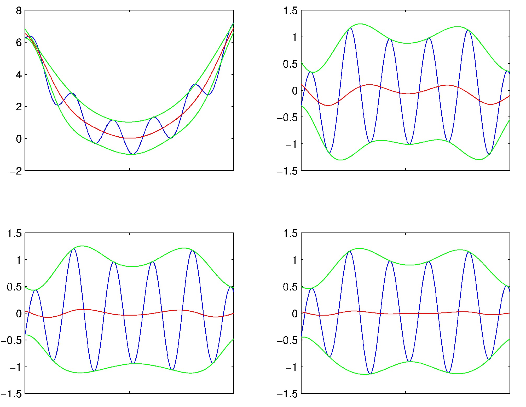
The core computation of EMD lies in the successive detection of maxima and minima in the time-series. These turning points are thence used to define upper and lower envelopes to the signal by fitting a spline curve which passes through the turning-point locations. The mid-point of these envelopes is then used as a baseline which is removed from the signal. This procedure is iterated until the baseline function is flat (to within a threshold). The resultant waveform at this point forms an intrinsic mode, which is then removed from the original time series. The entire process is then repeated, successively extracting intrinsic modes until the residual has no turning points.

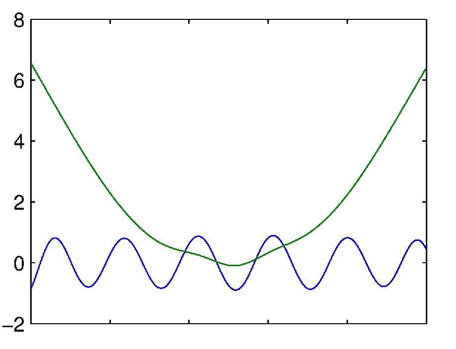
Figure 4 shows this process, which is referred to as sifting in the EMD literature, applied to a simple synthetic time-series. The example signal consists of a sine curve superimposed on a quadratic, as shown in the blue trace in the top left sub-figure. The green curves are the envelope functions at each iteration and the red trace is the mid-point baseline, which is subtracted from the time series at each iteration. We see that, even after a small number of iterations, the sine component is highlighted and this indeed forms the first intrinsic mode of the data. We continue this process until relative changes in the baseline function are $<10^{-3}$ (this results in some 20 iterations for the example shown here). Figure 5 shows both resultant intrinsic mode functions extracted from this data after iterating the sifting process until relative changes are below the threshold.

Figure 5: The two resultant intrinsic modes for the simple sine and quadratic example shown in Fig. 4.

2.4 Iterative trend identification and removal

Starting from the original set of light curves, the trend identification and removal proceeds as follows:

1. identify a set of candidate trends $\{\mathbf{\hat{d}}_{m}\}$, each associated with entropy $\mathcal{H}(\mathbf{w}_{m})$;

2. construct a candidate basis $\mathbf{T}$ from the 10 candidate trends with the highest entropy;

3. apply PCA to $\mathbf{T}$ and measure the spectral radius $\rho_{1}$ of its first principal component;

4. if $\rho_{1}<\rho_{\rm min}$, stop.

5. otherwise, perform EMD on the first principal component, and adopt the intrinsic mode with the largest variance as the next systematic trend $u_{k}$;

6. remove all the trends identified so far to produce a set of partially corrected light curves

   $$\mathbf{\tilde{d}}_{m}=\mathbf{d}_{m}-\sum_{k=1}^{K}a_{mk}\mathbf{u}_{k},$$ (8)

   where the $a_{mk}$ are once again found using VB with ARC priors.

7. return to step (i), with the $\{\mathbf{\tilde{d}}_{m}\}$ as inputs;

The process continues until $\rho_{1}<\rho_{\rm min}$ at step (iv).

The choice of stopping threshold $\rho_{\rm min}$ is a matter of fine-tuning. Typical values used in this work varied between 0.6 and 0.9, and the appropriate threshold was found by trial and error (i.e. by examining small subsets of the corrected light curves obtained using various values of $\rho_{\rm min}$). All the Kepler results presented in this paper used $\rho_{\rm min}=0.8$. We note that one could also select this threshold based on theoretical arguments. For example, recalling that the $\rho_{i}$’s are normalised eigenvalues of the matrix $\mathbf{TT^{\sf T}}$ (Eqs. 6 & 7), we can make use of the fact that the set of eigenvalues of an arbitrary matrix are bounded by the Weyl inequalities. For a large matrix, this can be extended to formulate probability distributions over the expected values in the presence of noise (Everson & Roberts, 2000). This could in principle be used to select $\rho_{\rm min}$ in a probabilistic manner. However, ultimately, the threshold will remain subjective, whether it is couched in terms of $\rho$, or a user-defined credibility limit in probability space. On balance, we felt that trial and error was the best means of ensuring that the choice of $\rho_{\rm min}$ reflects the all-important domain knowledge of the user.

The computational cost of the VB linear basis modelling done in step (i) scales as $M^{2}N$. It thus becomes prohibitive if $M$ is very large. When treating a large number of light curves, it is possible to decouple the trend identification and removal processes, using only a subset of the light curves for trend identification. This subset might be selected at random, or adjusted to contain light curves displaying evidence of systematics, but not strong intrinsic variability. The trend removal process scales more benignly as $MN$ and so can be applied easily even to large sets of light curves.

3 Results

In this section we apply the ARC method outlined above to two example datasets: first, a synthetic example for explanatory purposes, and the Kepler Q1 data, where we compare our results to the output of the existing PDC-MAP pipeline.

3.1 Synthetic example

In this subsection we present a simple synthetic example, to act as a ‘walk-through’ guide to the methodology and as a proof of concept.

We start with a set of 200 synthetic ‘light curves’ formed from random phase, frequency and amplitude sine curves, plus additive Gaussian noise. To these we add random amounts of two ‘systematic trends’: an exponential decay with long time constant, and a quadratic term. This constitutes our input dataset, examples of which may be seen in the top panel of Figure 6. Note that, without loss of generality, we normalise the curves such that each have unit variance and zero mean.

Figure 6: Application of the ARC to a synthetic dataset. Top panel: randomly chosen subset of input light curves. Second panel: the five highest entropy candidate trends found during the first iteration. Third panel: the first principal component of the high-entropy trends, which accounts for $>95$% of the variance. Bottom panel: the two basis trends discovered by the algorithm (solid lines) and the corresponding trends injected into the data (dashed lines); we note that the solid and dashed lines are almost undistinguishable as the recovered trends are very close to the originals.

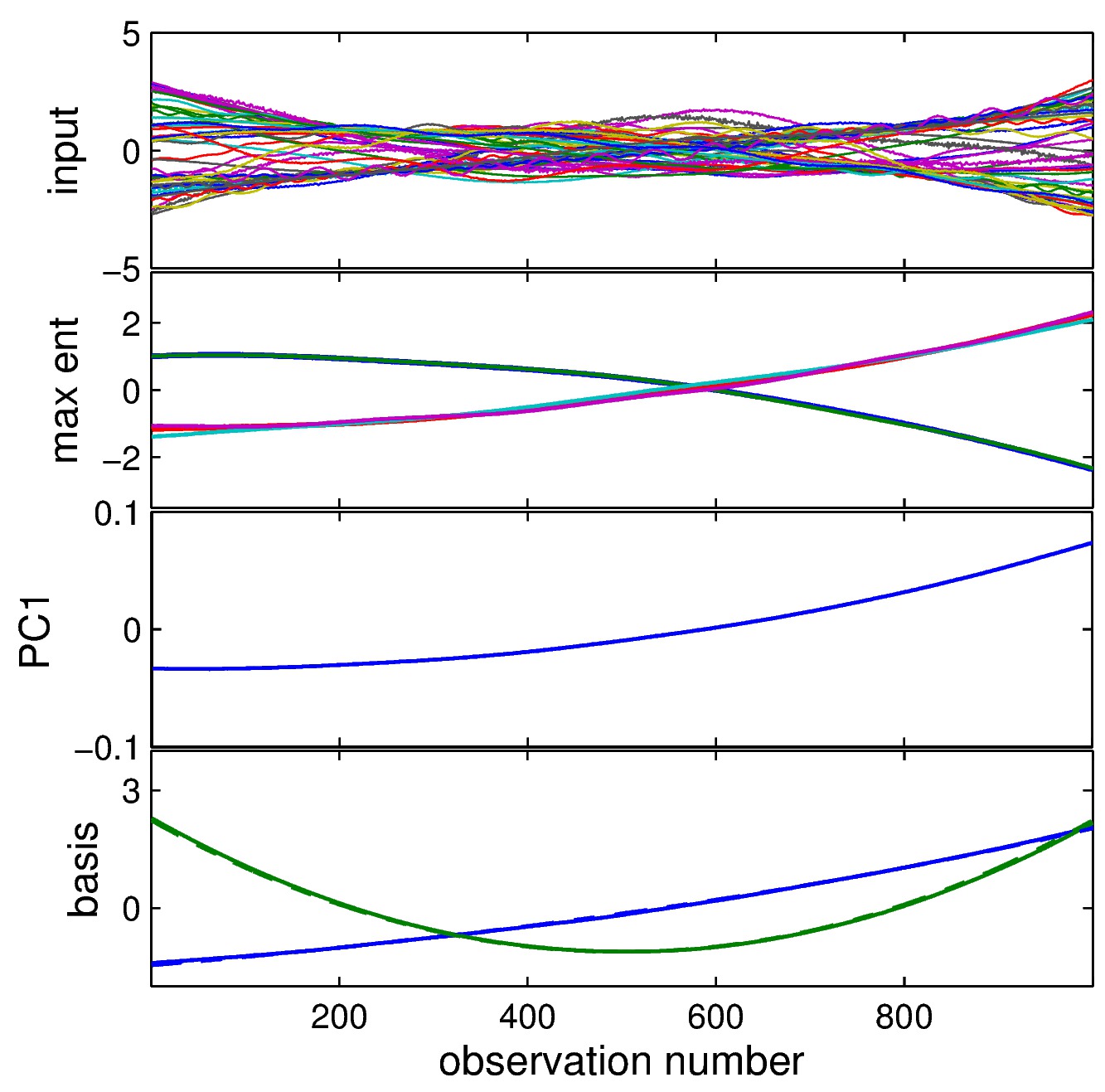
The steps of the method are illustrated in Figure 6. The trends were identified in a representative subset of 50 ‘light curves’ chosen at random, and the basis $\mathbf{T}$ was constructed from the ten highest-entropy trends at each iteration. Two systematic trends were identified before the stopping criterion was reached using $\rho_{\rm min}=0.6$. The resulting correction is illustrated on an example ‘light curve’ (not one of the subset in which the trends were identified) in Figure 7.

Figure 7: Result of the ARC applied to a synthetic dataset. Top panel: example ‘light curve’, with the systematics model (linear combination of the two identified trends) shown in red, and the actual trends injected in blue (with a vertical offset for clarity). Bottom panel: residuals after trend removal using the identified trends.

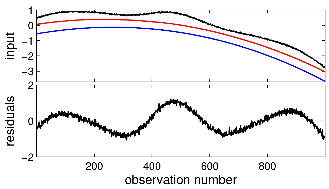
In this synthetic example we may compare the original data, prior to addition of systematic trend artefacts, with the recovered detrended traces, as we have the luxury of knowing the ‘ground truth’. The resultant linear correlations between the true ‘light curves’ and those recovered by the algorithm lie between 0.94 and 0.999, with a median value of 0.98, indicating a very high reconstruction accuracy (we note that the median correlation between the original curves and the trend-corrupted versions is only 0.11).

3.2 Application to Kepler Q1 data

We now apply the ARC to the first month of Kepler data, known as Q1. The ARC-corrected Q1 data were already used by McQuillan, Aigrain, & Roberts (2012) to study the statistics of stellar variability, but here we present a detailed description of the results and a comparison with the more recently released PDC-MAP data. The PDC-MAP data we use in this paper were made public on 25 April 2012 as part of Data Release 14, although the only significant difference between this and the earlier release of Q1 used by McQuillan, Aigrain, & Roberts (2012) is the replacement of the original PDC results with the output of the newer PDC-MAP pipeline. The data to which the ARC was applied are essentially the same.

The Q1 data consist of 1639 observations of 156 097 stars taken over 33.5 days in May–June 2009. The data we consider has been pre-processed only to convert it from pixel-level data to light curves, as described in Jenkins et al. (2010). The incident light is collected by 24 square modules, arranged to cover the focal plane of the telescope (Van Cleve & Caldwell, 2012). Each module consists of two rectangular charge-coupled device (CCD) detectors, each of which has two readout channels, resulting in a total of 84 channels and 94.6 million pixels.

Figure 8: Basis trends inferred from the global set of all Kepler Q1 light curves.

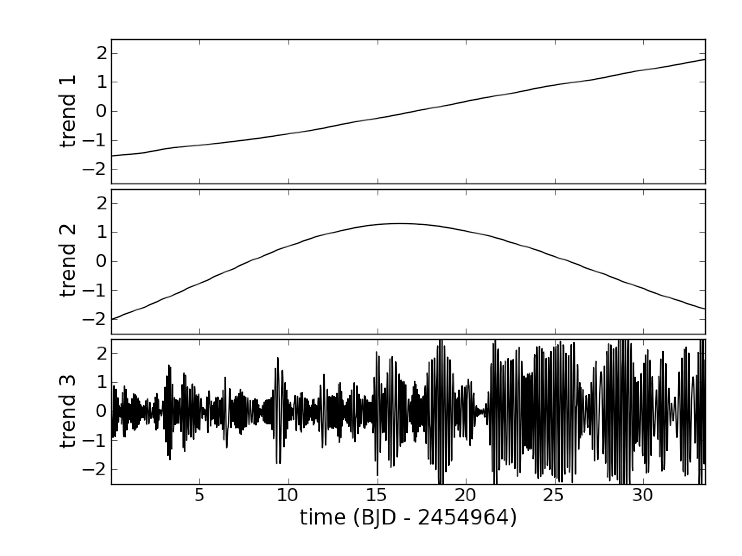
We first identified a single set of basis trends for all the light curves using a randomly selected subset of 200 light curves and using a threshold $\rho_{\rm min}=0.8$. These are shown in Figure 8. The first two have low-complexity, and are roughly linear and quadratic in nature, respectively. The third shows more complex dynamics, but is nonetheless present in a very large number of Q1 light curves. It is caused by the on/off switching of the reaction wheel heaters (Jenkins et al., 2013). We note that, although the first two trends resemble low-order polynomials, they are not simply linear and quadratic components. Furthermore, if we were to remove such low-order polynomials from each light curve individually, we would be failing to take into account the fact that the systematic trends are global rather than specific to each light curve.

Figure 9: Q1 trend basis sets inferred for each module (labelled in bold at the top left of each group of plots) and output channel (labelled at the bottom right of each panel). The blue, green, red, cyan, magenta, yellow and grey lines show trends 1 to 7 respectively (the number of trends identified varies). A vertical offset has been added between consecutive trends for clarity (the most important trend is always the lowest).

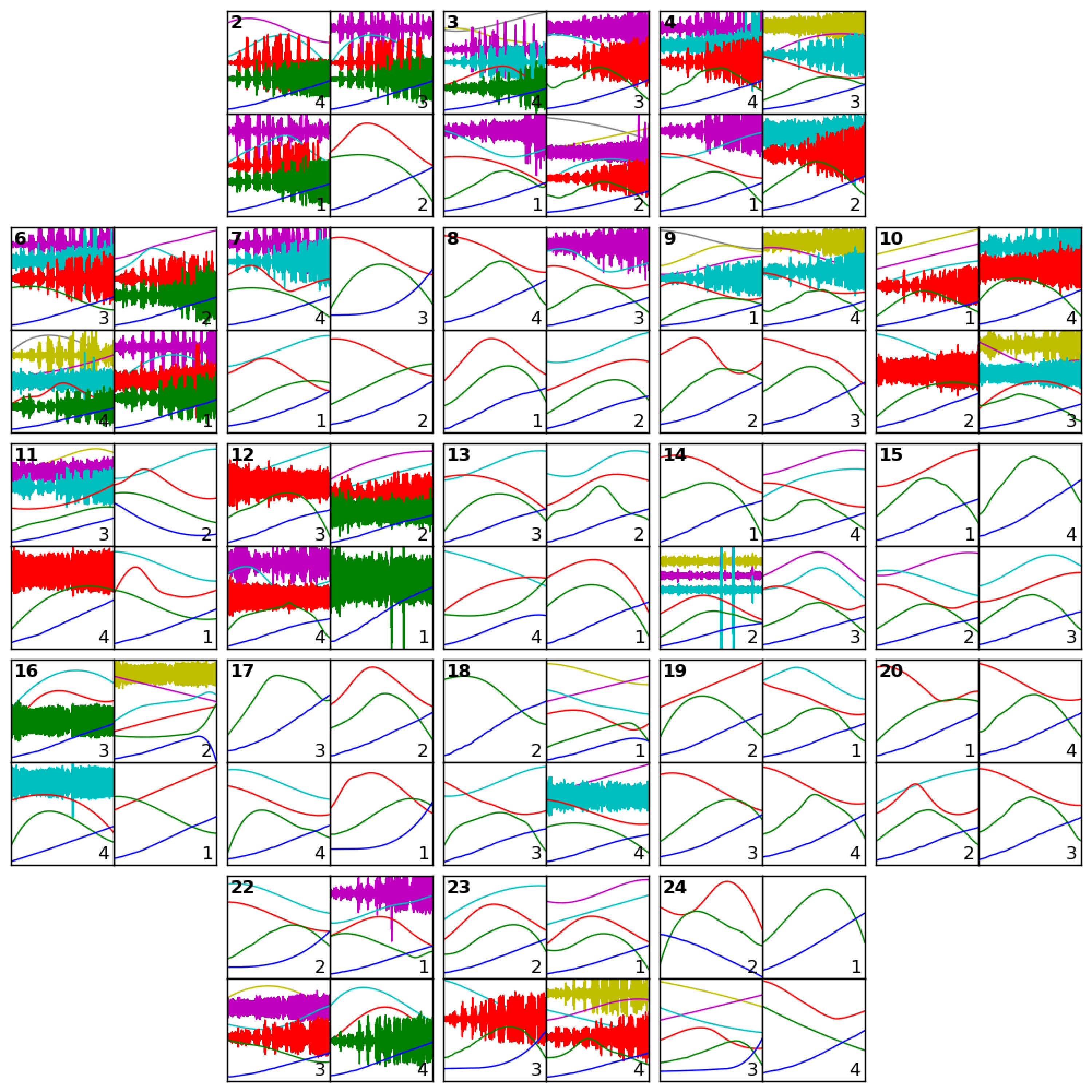
We then repeated the trend identification step, first on a module-by-module basis, then separately for each output channel. The basis trends identified in the latter case are shown in Figure 9. We compared the results from all three approaches, and ultimately settled on the output channel specific basis. The motivation for this is two fold. First, it is reasonable to expect that the systematics affecting the data collected on different detectors and read by different sets of electronics might differ, and visual examination of the corrected light curves appeared to bear this out, although the differences were very small.

Each of the Q1 light curves was then corrected using the set of basis trends identified for the corresponding output channel. The full set of basis trends and corrected light curves is available online at www.physics.ox.ac.uk/users/aigrain/KeplerSys/.

4 Discussion

Figure 10: Example results from Q1. Each row corresponds to a particlar object. In the left column, the raw data and the corrections applied by the PDC-MAP and ARC are shown in black, blue and red, respectively. The module and output channel number, KIC number of the target, and median flux in the raw light curve, are also shown. In the right column, the PDC-MAP and ARC corrected data are shown in blue and red respectively. Each light curve has been normalised by dividing them by their median and subtracting unity. A vertical offset has also been applied between the curves in each panel, to improve clarity.

In this section, we assess the performance of the ARC systematics correction on the Q1 data, and compare it to the PDC-MAP results.

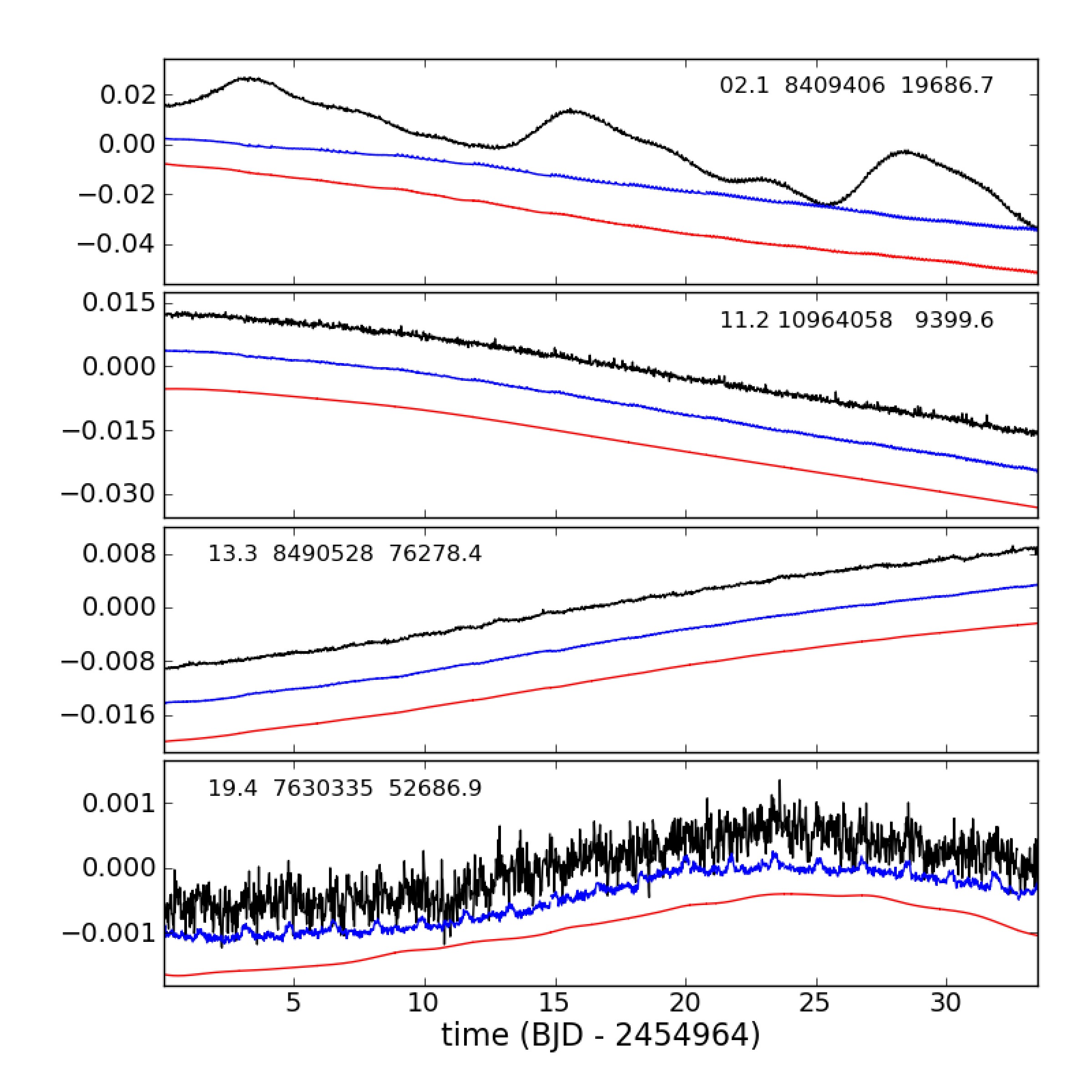
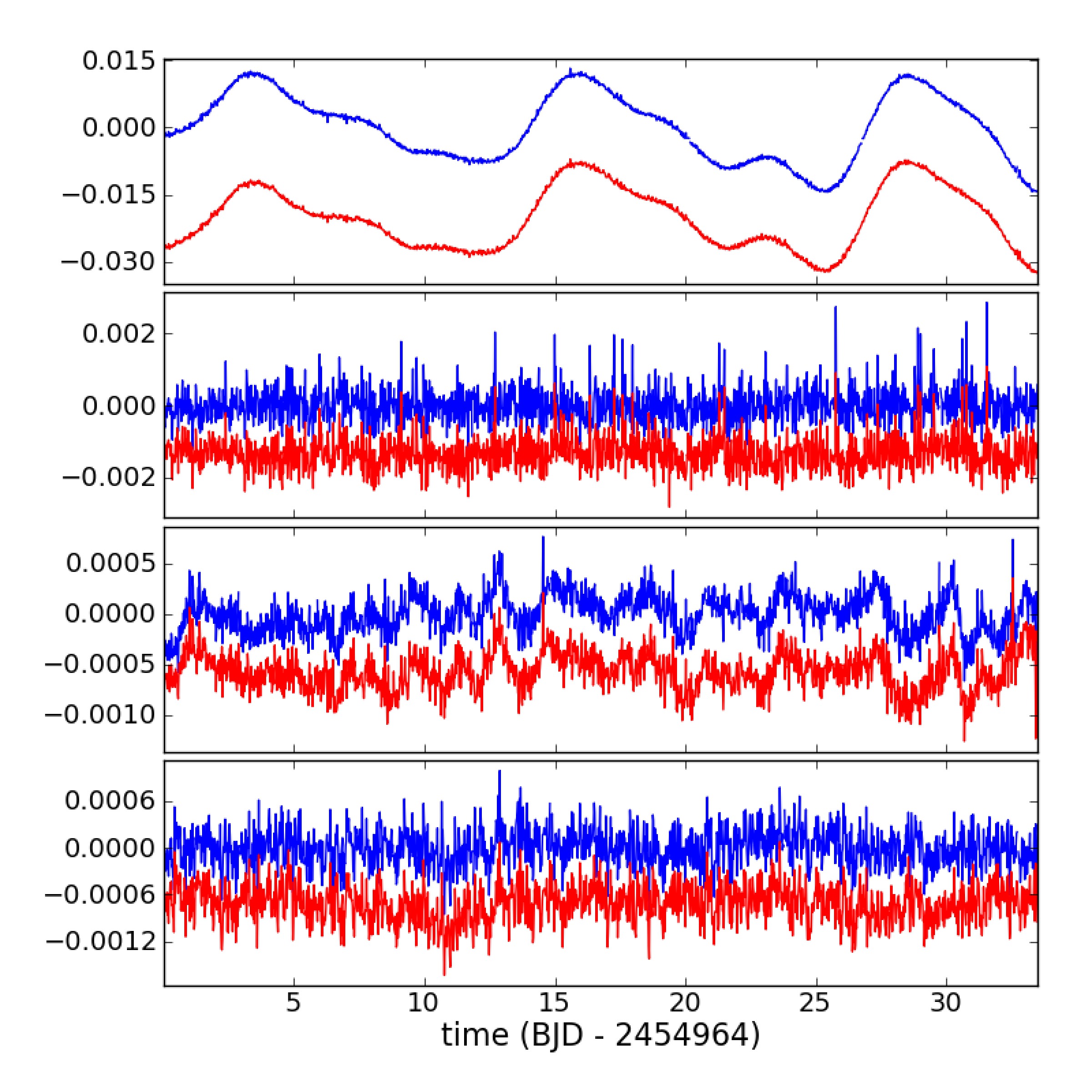
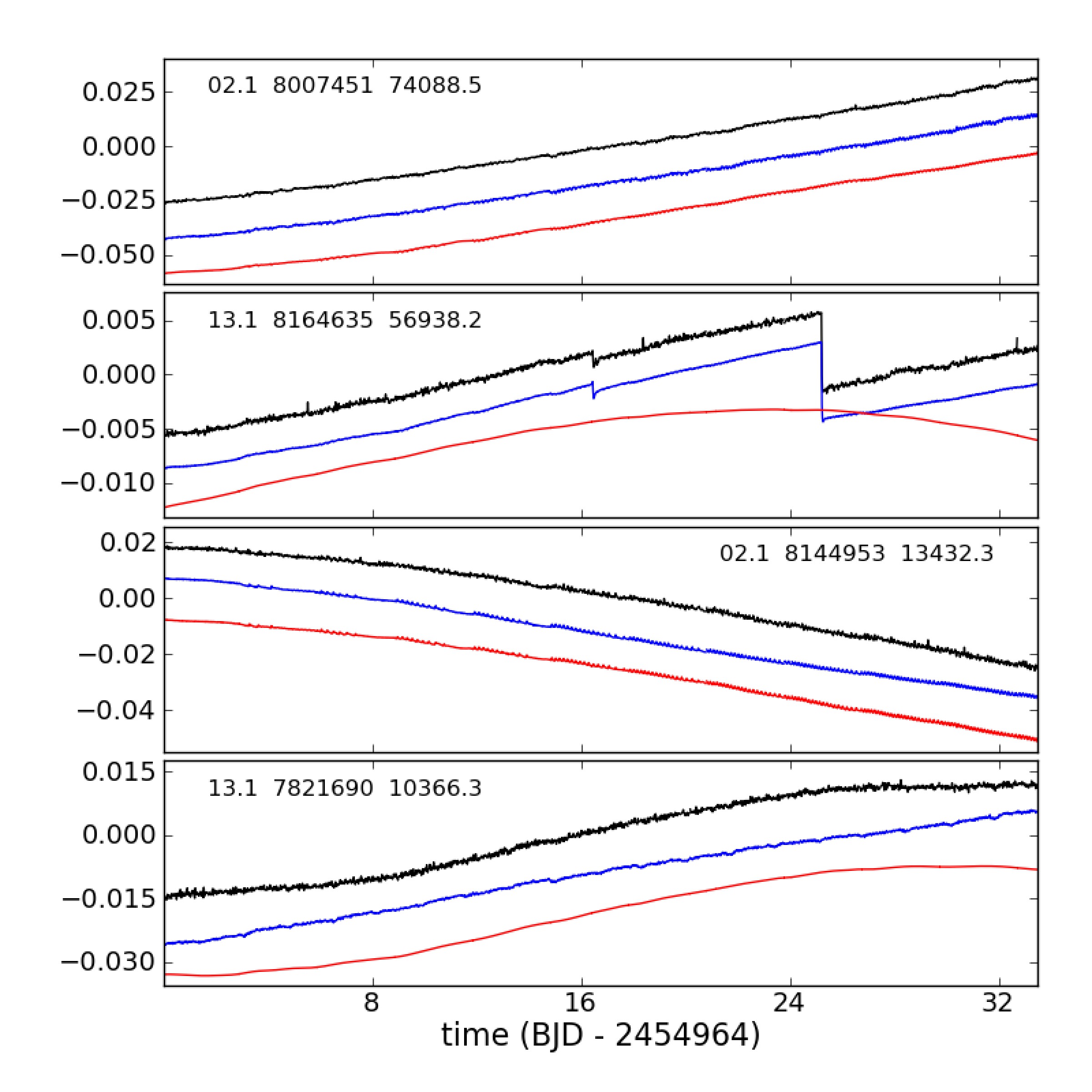
Figure 10 shows a selection of raw Q1 light curves along with the PDC-MAP- and ARC-corrected versions. These were selected at random on four different output channels in different parts of the detector, and are intended to represent a fairly typical subset of light curves, rather than a best- or worst-case scenario. The most striking outcome of the comparison is that the PDC-MAP and ARC results are, to first order, very similar. Both successfully preserve stellar variability in most cases, and remove most of the trends which one would deem to be systematic after visually inspecting many light curves.

Figure 11: Comparison of the light curve scatter on different timescales after correction by PDC-MAP and by the ARC. Each panel shows the ratio of the light curve scatter resulting from the two corrections as a function of the median flux in the light curve. The x-axis has been reversed (so brighter stars are to the left) and plotted on a log scale (so it is similar to a magnitude scale). The black points correspond to output channel 1 on module 2, where the ‘reaction wheel’ trend was found to be proeminent, and the red points to output channel 1 on module 13, near the centre of the detector, where only long-term trends were identifed.

However, there are some minor differences between the corrections applied by the PDC-MAP and the ARC. In the top panel of Figure 10, the low-frequency component of the applied corrections differs slightly. It is very difficult to determine, on a dataset of this duration, which correction is more appropriate. In the bottom panel, the PDC-MAP attempts to correct for the effect of periodic pointing anomalies caused by the presence of an eclipsing binary (EB) among the guide stars used in Q1. This is a known effect, which was remedied after Q1 (by eliminating the offending object from the set of guide stars). As we shall see below, although the EB signature is present among the basis vectors identified by the PDC-MAP pipeline, it remains challenging to correct. The EB signature is not captured at all by the ARC. It is visible in the candidate trends itendified for some (not all) of the output channels, before the EMD denoising step, but it is never represented in the intrinsic mode with the largest variance, which is adopted as the ‘smoothed’ basis trend. This is a limitation of our approach. More importantly, however, in this example the PDC-MAP also introduces significant amounts of high-frequency noise, which was not present in the original light curve. The EMD de-noising step avoids this, at the cost of failing to correct for the EB trend.

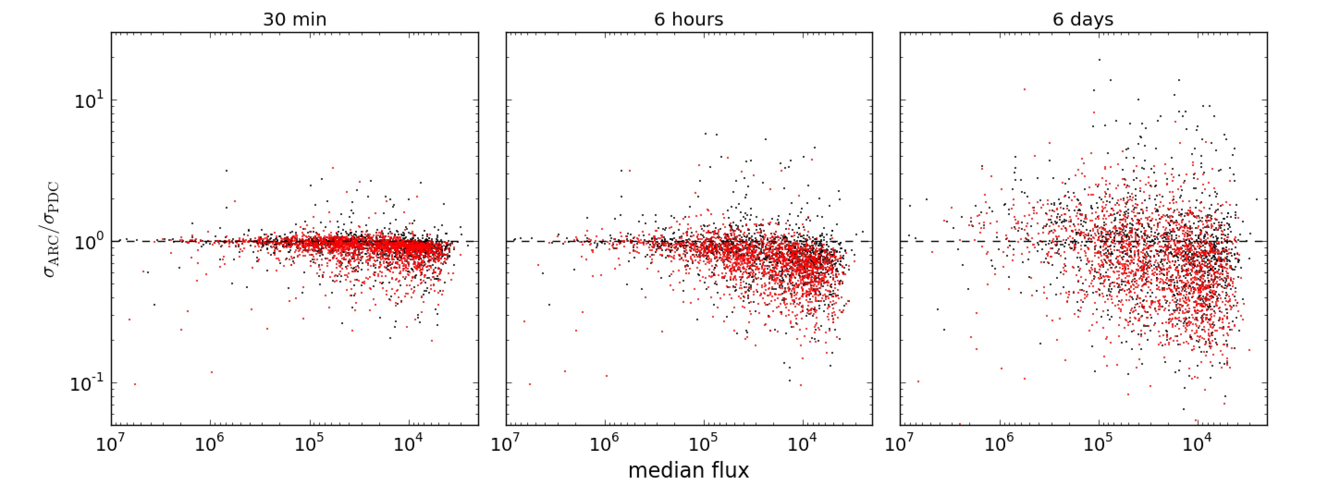
To investigate the differences between the PDC-MAP and ARC further, we computed the relative scatter of the corrected light curves on a range of timescales. We worked from the normalised light curves (after dividing them by the raw median flux), smoothed them on the timescale of interest using a median filter of the corresponding width, and estimated the scatter $\sigma$ as 1.48 times the median of the absolute deviations from unity. Figure 11 shows the ratio $\sigma_{\rm ARC}/\sigma_{\rm PDC}$ (where the subscript PDC refers to the PDC-MAP) as a function of the median flux, for two representative output channels (using all stars in each channel, namely 1290 and 2007 respectively), and for three different timescales: 30 minutes (the sampling of Kepler long-cadence observations), 6 hours (most relevant for transit detection, and 6 days (relevant, for example, to stellar rotation studies).

On all timescales, the ratio is below 1 for the majority of stars, meaning that the scatter of the ARC-corrected light curves is smaller than that of the PDC-MAP light curves. This effect is particularly noticeable for the fainter stars, where the scatters resulting from the two corrections often differ by a factor of 3 or more. At this stage, it would be tempting to interpret this as indicating that the PDC-MAP introduces some spurious signal into many of the light curves, which the ARC does not, presumably thanks to the de-noising step. Of course, we cannot entirely rule out the alternative possiblity that the ARC might be removing real astrophysical signal. However, it seems implausible that it would do systematically across a wide range of timescales, particularly because the ARD priors used at the trend removal stage ensure that trends are only removed if there is significant evidence for them in the data.

In order to verify that ARC is indeed removing only systematics, and that any alterations of the underlying (astrophysical) signals are minimal, we performed an injected signal test. We randomly selected 200 low-variability stars, displaying little other than white noise in their ARC-processed light curves, from mod2.out1. We added artificial sinusoidal signals (similar to those described in Section 3.1) to the raw light curves for these stars. We then used the ARC to identify a basis from to a set of light curves including some with injected signals and some without. This basis was then used to detrend both sets of light curves, allowing us to recover an estimate of the injected signals by subtraction. We then compared this to the actual injected signal in each case: any discrepancies must have been introduced by the ARC process. To quantify these discrepancies, we then evaluated, for each star, the variance of the residuals (the difference between the estimated and injected signals), divided by the variance of the injected signal. This is a quantitative measure of any discrepancy introduced by the ARC. We found that this discrepancy measure has a mean value of 1% and is never above 5%, confirming that the ARC procedure is unlikely to remove real astrophysical variability.

We also note that the number of cases, where the PDC-MAP and the ARC give very different scatters, increases at longer timescales. There are a few cases where the ARC scatter is significantly larger than the PDC-MAP value, and these are more numerous in the module 2 example than in the module 13 one.

Figure 12: Comparison of the ‘average’ power density spectra for bright stars before and after correction with the PDC-MAP and the ARC, in two representative output channels (top and bottom). The black, blue and red curves correspond to the raw, PDC-MAP and ARC data, respectively. The two columns show the same data, but the x-axis scale is logarithmic in one case, and linear in the other.

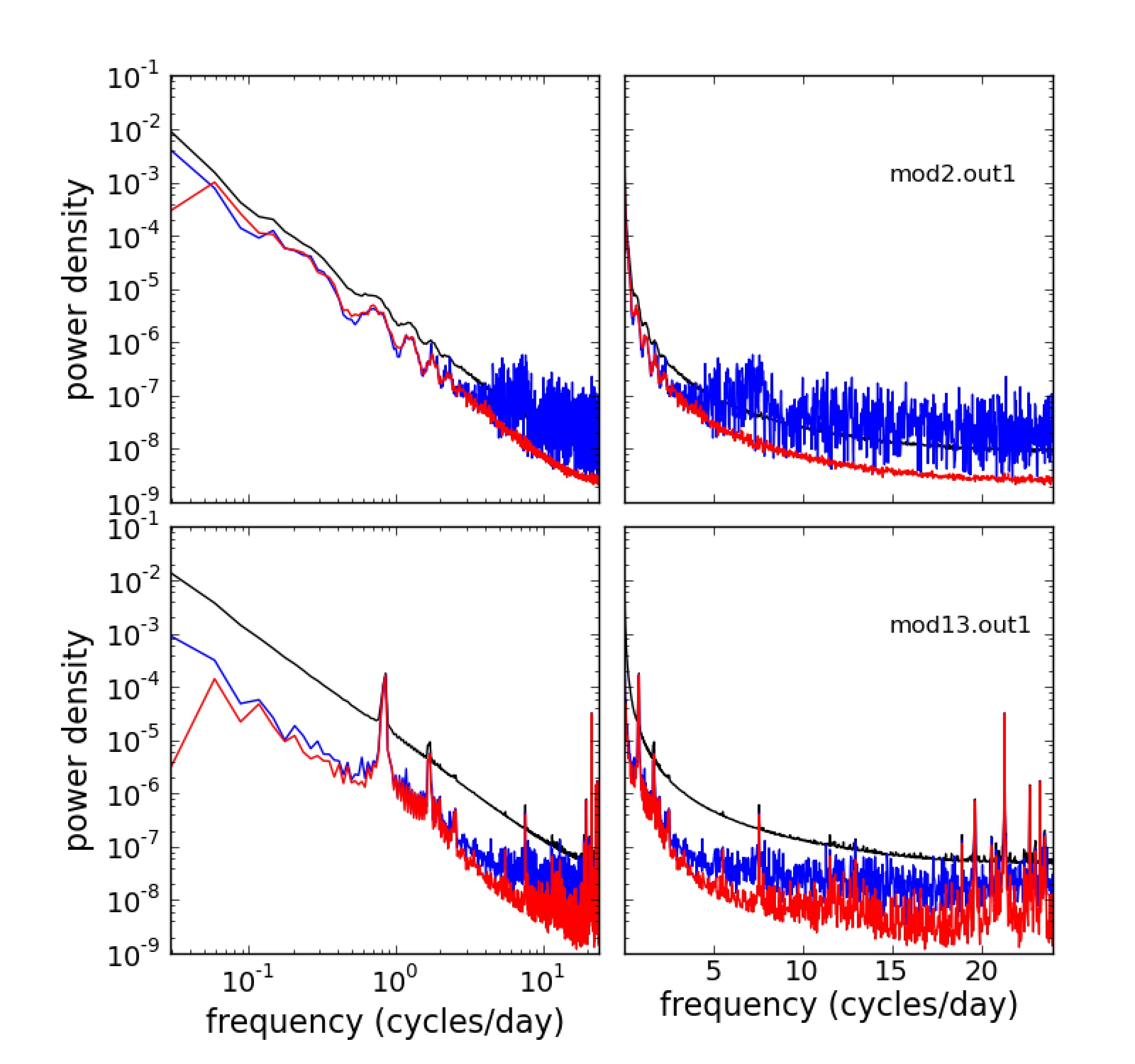
Gilliland et al. (2011) carried out an in-depth investigation of the noise properties of the PDC data. In particular, they showed that the majority of Sun-like stars observed by Kepler appear to display more variability on 6.5-hour timescales than the Sun. This is an important result, because it has a potentially serious impact on Kepler’s ability to detect transits of habitable planets. To estimate the variability on transit timescale, Gilliland et al. (2011) used a quantity known as the 6.5-hour combined differential photometric precision (CDPP). CDPP estimates computed by the Kepler pipeline itself are now publicly available and distributed with the Kepler data. Our 6-hour $\sigma$ estimates are not exactly identical to the CDPP values for the same dataset, because they are obtained in a slightly different fashion, but they do measure a similar quantity, namely the light curve scatter on typical transit timescales. Although improving the detectability of transits was not our primary motive in developing the ARC, the latter yields slightly lower scatter on transit timescales than the PDC, and hence the ARC may prove useful for transit searches.

We also computed ‘average’ power spectra before and after correction, for the bright stars (median raw flux $>10^{5}$ e^-/s) in the same two output channels (giving 56 and 69 stars for the two output channels respectively). These are simply averages of the individual power spectra of each light curve. The results are shown in Figure 12. Again, both systematics correction methods significantly reduce the light curve scatter on most timescales, and their behaviour is very similar at low frequencies (except for the very lowest, but these are poorly constrained due to the limited duration of the dataset). However, the power spectra conclusively demonstrate the fact that the PDC-MAP introduces high-frequency noise into the light curves (see also Murphy, 2012, though this reports results using PDC rather than PDC-MAP). This effect is more significant in some modules than in others, but the differences with the ARC become noticeable upwards of about 2 cycles per day. We note that, for mod2.out1, the set of systematics inferred by the ARC algorithm contains several high-frequency components. Similar trends may well be present in mod13.out1, but they are not significant in a large enough fraction of the light curves from that channel to be identified. This may explain the presence of excess power at high-frequencies in the average power spectrum of the ARC-corrected light curves from that channel, compared to mod2.out1. We ran a test where we arbitrarily fixed the number of trends identified to 5; this leads to the identification of the ‘reaction-wheel heater’ trend in most channels, but with very low spectral radius, indicating that it is not significant in the majority of light curves. This highlights the capricious trade-off between over- and under-fitting: in this work we have attempted to find a balance using the spectral radius threshold, but other choices are possible.

The power spectra shown in the bottom panel of Figure 12 correspond to the central module of the Kepler detector, where the only trends identified by the ARC were long-term. There are clearly systematic effects at well-defined frequencies, which are not well captured by either the PDC-MAP or the ARC. The signal at $\sim 0.8$ cycles/day and harmonics thereof correspond to the aforementioned EB guide star; there are also a number of higher-frequency effects. The fact that neither the PDC-MAP nor the ARC correct these effects well suggests that they may not obey one of the fundamental assumptions underlying both methods. For example, if the contribution of a given trend to a given light curve varies during the quarter, the linear basis model will not be able to capture it.

There are also some interesting differences in the average power at a given frequency, and in the relative reduction in this power introduced by the systematics corrections, for the two output channels shown. However, it would probably be unwise to read too much into this, as these power spectra are based on relatively small numbers of light curves ($\sim 50$ in each case). Another point which we note as interesting, but refrain from discussing further, is that all the power spectra – before and after systematics correction of any kind – are remarkably well-described by power laws with index $-2$, as expected for an auto-regressive stochastic process, and frequently used to model the so-called ‘solar background’ (Harvey 1985. See McQuillan, Aigrain, & Roberts 2012 for a more detailed discussion of this aspect).

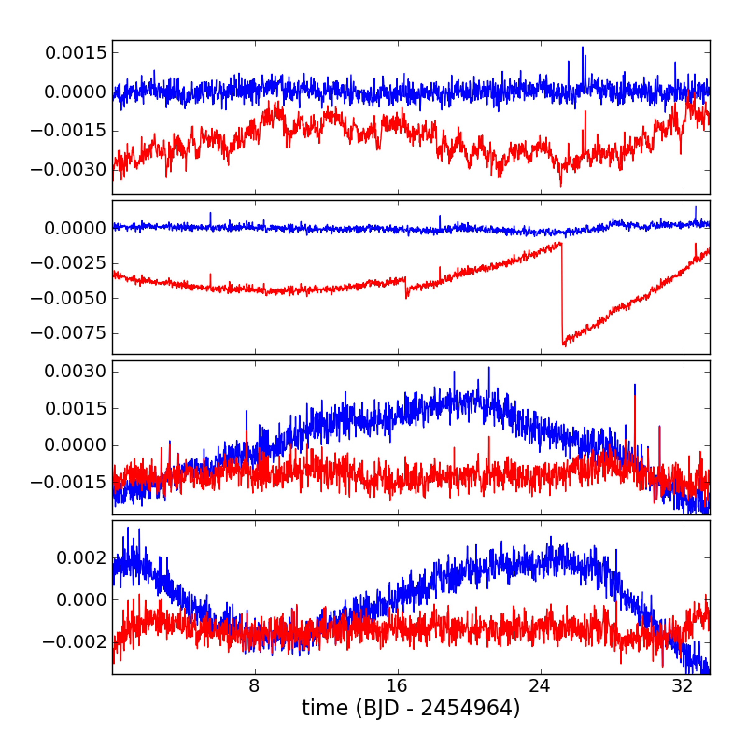
There are a few larger differences between the ARC and PDC-MAP corrections. In Figure 13 we highlight representative, but rare, examples of large deviations. The top two examples show cases where the post-ARC scatter is larger than the post-PDC scatter (by a factor of $>2$ on 30 min timescales, $>3$ on 6 hr timescales and $>5$ on 6 day timescales). In both cases the light curve contains a strong signature of an effect that the ARC cannot deal with, for example the binary guide star (top row) or strong discontinuities (pixel sensitivity drop-outs, 2nd row). The bottom two examples show cases where the post-ARC scatter is considerably smaller than the post-PDC scatter (by a factor of $>3$ on 30 min timescales, $>5$ on 6 hr timescales and $>10$ on 6 day timescales). In both cases this is because the range of basis vectors available in the PDC-MAP detrending algorithm does not explain the light curve as effectively as the ARC.

It is important to highlight two points regarding these deviations. Firstly, the cases where post-ARC scatter is significantly larger than the post-PDC-MAP scatter are much rarer than vice versa. Secondly, the effects the ARC method cannot currently deal with are either not present in later quarters (e.g. the eclipsing binary guide star) or will be dealt with separately by utilising jump-correction software, developed primarily for quarter 2 analysis, which will be described in a later paper.

Figure 13: Example results from Q1 where there are significant deviations between the ARC and PDC-MAP detrended light curves. Each row corresponds to a particlar object. In the left column, the raw data and the corrections applied by the PDC-MAP and ARC are shown in black, blue and red, respectively. The module and output channel number, KIC number of the target, and median flux in the raw light curve, are also shown. In the right column, the PDC-MAP and ARC corrected data are shown in blue and red respectively. Each light curve has been normalised by dividing them by their median and subtracting unity. A vertical offset has also been applied between the curves in each panel, to improve clarity. In the top two examples post-ARC scatter is larger than that from PDC-MAP correction and in the lower two it is less.

5 Conclusions

We have presented a novel method to correct systematic trends present in large ensembles of light curves, while preserving ‘true’ astrophyiscal variability, which we call the ARC method. The ARC is specifically designed for continuous, high-precision observations, where most stars display significant variability. It follows established practice in using linear basis models, but incorporates a number of new features, which are intended to ensure its robustness (Bayesian framework, use of shrinkage priors), and its computational efficiency (approximate inference using variational Bayes). A de-noising step is used to prevent the introduction of spurious random noise into the light curves.

We demonstrated the performance of the method on a simple synthetic dataset, and on the data from the first month of Kepler operations. The results were satisfactory in both cases. In the synthetic example, the systematic trends were correctly identified. The original light curves included the building blocks of realistic stellar signals, namely harmonic functions with random, variable phases and amplitudes, and were recovered robustly, with no evidence of systematic changes in amplitude or frequency. For the Kepler data, the ARC results are similar to those of the PDC-MAP component of the Kepler pipeline for most targets, but with some important differences. In particular, we find that the PDC-MAP still tends to introduce high-frequency noise into the light curves (just as noted by Murphy 2012 for the original PDC). Importantly, this effect remains noticeable on the timescales typical of planetary transits. To address this problem, the Kepler team recently developed a new incarnation of the PDC, known as multi-scale MAP, or msMAP for short (DR21, 2013), which uses a band-splitting approach to separate systematics on different timescales. This does reduce the injection of high-frequency noise into the light curves compared to the PDC-MAP. However, in msMAP the treatment of long-term systematics (on timescales $\geq 21$ days) has reverted to the maximum likelihood approach of the original PDC pipeline. Consequently there is no protection against overfitting, and msMAP suppresses all variations on timescales longer than $\sim 20$ days – whether astrophysical or instrumental (see Fig. 1 in DR21, 2013). Therefore, although we have not had the opportunity to make a detailed comparison between the new msMAP data and the ARC, we expect the letter to be preferrable for variability studies.

We did, however, identify certain types of systematics which are not well-corrected by either the PDC-MAP or ARC. Further work needs to be done on these: one area in particular which could be improved is the de-noising step, as the EMD method used for that step in the present paper is not suitable for sharp systematic effects. Another possibility, which we intend to investigate, is to treat the systematics as multiplicative, rather than additive, by working in log flux units. This which would account for gradual amplitude changes, which could occur due to the combined effect of pixel drift and aperture contamination (if one of the stars in the aperture is more variable than the other). The impact of the residual systematic effects should be relatively limited, because they are confined to well-defined frequency ranges. Overall, we therefore conclude that the ARC-corrected light curves could become a very useful resource for both stellar astrophysics and exoplanet searches, and we have made the Q1 data publicly available (the code is also available on request).

However, the full potential of the Kepler data lies in its very long baseline. This paper focused on the first month of data only, whereas more than three years are now in the public domain. A number of additional difficulties arise when trying to process the additional quarters, and to stitch together multiple quarters. Many of the quarters contain discontinuities, most of which are associated with monthly interruptions in the observations to transfer data back to Earth. Many of the discontinuities are followed by quasi-systematic trends which are present in most light curves, but with slightly different shapes. As the satellite rotates by $90^{\circ}$ about its viewing axis between each quarter, each star falls on a different detector, and this causes changes in both the median flux level and the nature and amplitude of the systematic trends. The ARC is not designed to address these problems. We are in the process of developing a complementary set of ‘fault-correction’ tools, to be applied on a light-curve by-light-curve basis before running the ARC on each channel. The same methodology can then be used to stitch together data from different quarters. These developments will be covered in a forthcoming paper.

As a final cautionary note, we wish to stress that the ARC is intended to provide a fast, automated and robust treatment of a large ensemble of light curves. It is not intended to replace the detailed examination of the pixel-level data (Kinemuchi et al., 2012; Harrison et al., 2012), which remains the method of choice for the correction of systematic trends and artefacts in small numbers of light curves.

Appendix A Bayesian Linear Basis Model

In a general linear basis model, the observations of a dependent variable are modelled as a linear combination of basis functions of an independent variable, plus a noise term. For consistency with the notation used in the rest of the paper, we call the independent variable $t$ and the dependent variable $d$, so that:

$$d(t)=\sum_{k=1}^{K}w_{k}\phi_{k}(t)+\epsilon,$$ (9)

where the $w$’s are known as the factor weights and the $\phi$’s are the basis functions. The noise term, $\epsilon$, is taken to be drawn from a normal (Gaussian) distribution with zero mean and precision (inverse variance) $\beta$. Note that an offset, or bias term, can easily be included in the model by including a basis function which is one everywhere.

Defining the column vectors $\mathbf{w}\equiv[w_{1}$, …, $w_{K}]^{\sf T}$ and $\mbox{\boldmath$\phi$}(t)\equiv[\phi_{1}(t)$, …, $\phi_{K}(t)]^{\sf T}$, we can re-write Equation (9) as:

$$d(t)=\mathbf{w}^{\sf T}\mbox{\boldmath$\phi$}(t)+\epsilon.$$ (10)

We then obtain a system of simultaneous linear equations describing the dataset as a whole:

$$\mathbf{d}=\mathbf{w}^{\sf T}\mbox{\boldmath$\Phi$}+\mbox{\boldmath$\epsilon$},$$ (11)

where $\mathbf{\Phi}$ is an $N\times K$-element matrix with elements $\phi_{k}(t_{n})$ and $\mbox{\boldmath$\epsilon$}\equiv[\epsilon_{1}$, …, $\epsilon_{N}]^{\sf T}$.

The likelihood, i.e. the probability that our model gave rise to the observations, is then simply

$$p(d|\mathbf{w},\beta)=\mathcal{N}(\mathbf{d};\mathbf{w}^{\sf T}\mbox{\boldmath$\Phi$},\beta^{-1}\mathbf{I})$$ (12)

where $\mathcal{N}(\mathbf{a};\mathbf{b},\mathbf{C})$ is the probability of drawing a vector $\mathbf{a}$ from a multi-variate Gaussian distribution with mean vector $\mathbf{b}$ and covariance matrix $\mathbf{C}$, and $\mathbf{I}$ is the identity matrix.

A.1 Maximum Likelihood

The maximum likelihood (ML) solution for the weights is given by the standard pseudo-inverse equation, namely

$$\mathbf{w}_{\rm ML}=(\mbox{\boldmath$\Phi$}^{\sf T}\mbox{\boldmath$\Phi$})^{-1}\mbox{\boldmath$\Phi$}^{\sf T}\mathbf{d}.$$ (13)

However, the ML approach is prone to over-fitting. Some relief from the inherent problems associated with ML solutions may be obtained by introducing a prior over the weights and obtaining the maximum a posteriori (MAP) solution. This approach still relies on point estimates of the parameters of the models, and consequently fails to take into account some of the intrinsic uncertainties.

A full Bayesian solution is obtained by marginalising over the posterior distributions of the variables, which can be achieved, for example, using sample-based approaches such as Markov-Chain Monte-Carlo (MCMC). These can be computationally intensive however, and they scale poorly to large numbers of parameters, and it is often problematic to establish whether convergence has been reached. In this paper, we advocate an alternative solution based on the variational Bayes (VB) framework. In recent years VB has been extensively used in the machine learning literature as a method of choice for approximate Bayesian inference, as it offers computational tractability even on very large data sets. A full tutorial on VB is given in Bishop (2006); Fox & Roberts (2011). In what follows we describe the key features and concentrate on the derivations of update equations for the linear basis model at the core of this paper.

A.2 The full Bayesian model

In a Bayesian framework, the priors over the parameters of the model must be specified. For each of the weights, a zero-mean Gaussian prior with precision $\alpha$ is adopted. The zero mean ensures that the weight associated with a given basis function is only non-zero if the data requires it to be. The Gaussian is the least informative choice of distribution for a quantity that can be either positive or negative, and is therefore appropriate when little information is known about the weights a priori. It is also convenient to chose a form for the prior that is conjugate with the likelihood, because it makes the marginalization process analytic. The joint prior over all the weights is thus:

$$p(\mathbf{w}|\alpha)=\mathcal{N}(\mathbf{w};\mathbf{0},\alpha^{-1}\mathbf{I}).$$ (14)

The value of $\alpha$ does not enter into the likelihood, but it does control the parameters, and it is therefore known as a hyper-parameter. In a fully Bayesian treatment, rather than fixing $\alpha$ to a specific value, we marginalise over it, under a so-called hyper-prior. It is convenient to select a hyper-prior for $\alpha$ that is conjugate with the prior over the weights, because then the marginalisation can be done analytically. As the prior is a Gaussian, and $\alpha$ should always be positive (because it represents an inverse variance), a suitable form for the hyper-prior is a Gamma distribution with shape parameter $a$ and scale parameter $b$:

$$p(\alpha)=\mathcal{G}(\alpha;a,b)\equiv\frac{1}{\Gamma(a)b^{a}}\,\alpha^{a-1}\,e^{-\alpha/b},$$ (15)

where $\Gamma(x)$ is the Gamma function.

The noise precision, $\beta$, is also a parameter of the model, for which we need to adopt a prior. Again, a Gamma distribution is a suitable choice, with hyperparameters $c,d$:

$$p(\beta)=\mathcal{G}(\beta;c,d).$$ (16)

We concatenate all the parameters and hyperparameters of the model into the vector $\mbox{\boldmath$\theta$}=[\mathbf{w},\alpha,\beta]^{\sf T}$. As the weights depend upon the scale $\alpha$ but not the noise precision $\beta$ the joint prior distribution over $\theta$ factorises as:

$$p(\mbox{\boldmath$\theta$})=p(\mathbf{w}|\alpha)\,p(\alpha)\,p(\beta).$$ (17)

Our objective in Bayesian regression is to estimate the posterior distribution, which fully describes our knowledge regarding the parameters of the model, $\theta$, given the data $\mathbf{d}$. This is related to the likelihood and prior by Bayes’s theorem:

$$p(\mbox{\boldmath$\theta$}|\mathbf{d})=\frac{p(\mathbf{d}|\mbox{\boldmath$\theta$})\,p(\mbox{\boldmath$\theta$})}{p(\mathbf{d})}.$$ (18)

The denominator is the evidence or marginal likelihood of the data under the model, and is given by

$$p(\mathbf{d})=\int p(\mathbf{d}|\mbox{\boldmath$\theta$})\,p(\mbox{\boldmath$\theta$})\,\mathrm{d}\mbox{\boldmath$\theta$}$$ (19)

More than a mere normalisation term, the evidence is a quantitative measure of the extent to which the data supports the model.

Appendix B Variational Bayesian Inference

Whether we are interested in the model evidence or in the posterior distribution over individual parameters (after marginalising over the others), the functional dependence of the likelihood and posterior distribution on the parameters are generally unknown. However, we can propose an analytical approximation for any one of them, which can if necessary be refined later. This gives rise to the class of approximate inference methods.

In variational inference, we introduce an analytically tractable distribution $q(\mbox{\boldmath$\theta$}|\mathbf{d})$, which we use to approximate the posterior distribution $p(\mbox{\boldmath$\theta$}|\mathbf{d})$. We use this to write the log evidence as the sum of two separate terms:

$$\log p(\mathbf{d}) = \log p(\mathbf{d})\int q(\mbox{\boldmath$\theta$}|\mathbf{d})\,\mathrm{d}\mbox{\boldmath$\theta$}$$ (20)

$$= \int q(\mbox{\boldmath$\theta$}|\mathbf{d})\,\log p(\mathbf{d})\,\mathrm{d}\mbox{\boldmath$\theta$}$$ (21)

$$= \int q(\mbox{\boldmath$\theta$}|\mathbf{d})\,\log\left[\frac{p(\mathbf{d},\mbox{\boldmath$\theta$})}{p(\mbox{\boldmath$\theta$}|\mathbf{d})}\right]\,\mathrm{d}\mbox{\boldmath$\theta$}$$ (22)

$$= \int q(\mbox{\boldmath$\theta$}|\mathbf{d})\,\log\left[\frac{p(\mathbf{d},\mbox{\boldmath$\theta$})}{p(\mbox{\boldmath$\theta$}|\mathbf{d})}\cdot\frac{q(\mbox{\boldmath$\theta$}|\mathbf{d})}{q(\mbox{\boldmath$\theta$}|\mathbf{d})}\right]\,\mathrm{d}\mbox{\boldmath$\theta$}$$ (24)

$$= \int q(\mbox{\boldmath$\theta$}|\mathbf{d})\log\frac{p(\mathbf{d},\mbox{\boldmath$\theta$})}{q(\mbox{\boldmath$\theta$}|\mathbf{d})}~{}\mathrm{d}\mbox{\boldmath$\theta$}$$

$$\hskip 28.45274pt-\int q(\mbox{\boldmath$\theta$}|\mathbf{d})\log\frac{p(\mbox{\boldmath$\theta$}|\mathbf{d})}{q(\mbox{\boldmath$\theta$}|\mathbf{d})}~{}\mathrm{d}\mbox{\boldmath$\theta$}$$

$$\equiv \mathcal{F}(p,q)+{\rm KL}(p,q).$$ (25)

Equation 25 is the fundamental equation of the VB-framework. The first term on the right-hand side, $\mathcal{F}(p,q)$, is known as the (negative) variational free energy. The second, ${\rm KL}(p,q)$ is the Kullback-Leibler (KL) divergence between the approximate posterior $q$ and the true posterior $p$. Importantly, the KL divergence is always positive. $\mathcal{F}(p,q)$ thus provides a strict lower bound on the log evidence. Moreover, because the KL divergence is zero when the two densities are the same, $\mathcal{F}(p,q)$ will become equal to the log evidence when the approximating posterior is equal to the true posterior, i.e. when $q(\mbox{\boldmath$\theta$}|\mathbf{d})=p(\mbox{\boldmath$\theta$}|\mathbf{d})$. The aim of VB learning is therefore to maximise $\mathcal{F}(p,q)$ and so make the approximate posterior as close as possible to the true posterior. This requires the extremisation of an integral with respect to a functional, which is typically achieved using the calculus of variations.

However, to obtain a practical inference algorithm, we restrict the range of proposal posterior distributions over which we perform the optimization. First, we restrict ourselves to distributions belonging to the exponential family. This ensures that extremisation over the function $q(\mbox{\boldmath$\theta$})$ can be replaced exactly by extremisation with respect to the parameters $\theta$. As this family includes all the commonly-used probability distributions, this constraint is not normally problematic. What we obtain is then a set of coupled update equations over the parameters which are cycled until a convergence criterion is met. This approach is a generalisation of the expectation-maximisation (EM) algorithm, which is obtained as a special case of variational Bayes in the limit of the $q()$ distributions being replaced by delta functions at their maximum-likelihood values (Bishop, 2006).

Furthermore, we also assume that the posterior distribution is separable, meaning that it can be written as a product of independent functions of different parameters (or subsets of the parameters). This makes the resultant inference algorithm computationally very rapid, with little loss of information.

We begin by writing this factorisation as:

$$q(\mbox{\boldmath$\theta$}|\mathbf{d})=\prod_{i}q(\theta_{i}|\mathbf{d}).$$ (26)

This makes the resultant inference algorithm computationally very rapid, with little loss of information. The aim is to find the distribution $q(\mbox{\boldmath$\theta$}|\mathbf{d})$ for which $\mathcal{F}(p,q)$ is largest, which is done by optimising each of the factors in turn. We start by substituting this separable expression into $\mathcal{F}(p,q)$:

$$\mathcal{F}(p,q)=\int\prod_{i}q(\theta_{i}|\mathbf{d})\left[\log p(\mathbf{d},\mbox{\boldmath$\theta$})-\sum_{i}\log q(\theta_{i}|\mathbf{d})\right]\mathrm{d}\mbox{\boldmath$\theta$}.$$ (27)

Next, we write down separately the terms which depend on one of the parameters, $\theta_{j}$:

$$\mathcal{F}(p,q) = \iint\mathrm{d}\theta_{j}\mathrm{d}\mbox{\boldmath$\theta_{(i\neq j)}$}\,q(\theta_{j}|\mathbf{d})\prod_{i\neq j}q(\theta_{i}|\mathbf{d})\$$

$$\times \left[\log p(\mathbf{d},\mbox{\boldmath$\theta$})-\log q(\theta_{j}|\mathbf{d})-\sum_{i\neq j}\log q(\theta_{i}|\mathbf{d})\right].$$

We then rearrange the above equation, so as to isolate the dependency on $\theta_{j}$:

$$\mathcal{F}(p,q) = \int q(\theta_{j}|\mathbf{d})\,\left\{\int\log p(\mathbf{d},\mbox{\boldmath$\theta$})\,\right.$$ (29)

$$\times \left.\prod_{i\neq j}q(\theta_{i}|\mathbf{d})\,\mathrm{d}\mbox{\boldmath$\theta_{(i\neq j)}$}\right\}\,\mathrm{d}\theta_{j}$$

$$- \int q(\theta_{j}|\mathbf{d})\,\log q(\theta_{j}|\mathbf{d})\,\mathrm{d}\theta_{j}\,\int\prod_{i\neq j}q(\theta_{i}|\mathbf{d})\,\mathrm{d}\mbox{\boldmath$\theta_{(i\neq j)}$}$$

$$- \int\prod_{i\neq j}q(\theta_{i}|\mathbf{d})\sum_{i\neq j}\log q(\theta_{i}|\mathbf{d})\,\mathrm{d}\mbox{\boldmath$\theta_{(i\neq j)}$}$$

$$\times \int q(\theta_{j}|\mathbf{d})\,\mathrm{d}\theta_{j}.$$

The second factor in each of the last two terms in Equation (29) is the integral of a probability distribution, and is thus equal to one. Furthermore, the third term is independent of $\theta_{j}$, so:

$$\mathcal{F}(p,q) = \int q(\theta_{j}|\mathbf{d})\,\left\{\int\log p(\mathbf{d},\mbox{\boldmath$\theta$})\,\prod_{i\neq j}q(\theta_{i}|\mathbf{d})\,\mathrm{d}\mbox{\boldmath$\theta_{(i\neq j)}$}\right\}\,\mathrm{d}\theta_{j}$$ (30)

$$- \int q(\theta_{j}|\mathbf{d})\,\log q(\theta_{j}|\mathbf{d})\,\mathrm{d}\theta_{j}\,+{\mbox{const}}(j)$$

where ${\mbox{const}}(j)$ represents a term that is constant with respect to $\theta_{j}$. The quantity in curly braces in the first term of Equation (30) is the expectation of $\log p(\mathbf{d},\mbox{\boldmath$\theta$})$ under the candidate posterior distribution for all the other parameters, $\prod_{i\neq j}q(\theta_{i}|\mathbf{d})$. We wish to isolate the part of it which depends on $\theta_{j}$. To this end, we define the quantity

$$f(\theta_{j})\stackrel{{\scriptstyle\mbox{\tiny def}}}{{=}}\int\log\left[p(\mathbf{d},\mbox{\boldmath$\theta$})\right]_{j}\,\prod_{i\neq j}q(\theta_{i}|\mathbf{d})\,\mathrm{d}\mbox{\boldmath$\theta_{(i\neq j)}$},$$ (31)

where $\left[p(\mathbf{d},\mbox{\boldmath$\theta$})\right]_{j}$ contains all the terms in $p(\mathbf{d},\mbox{\boldmath$\theta$})$, which depend on $\theta_{j}$. We can then write

$$\int\log p(\mathbf{d},\mbox{\boldmath$\theta$})\,\prod_{i\neq j}q(\theta_{i}|\mathbf{d})\,\mathrm{d}\mbox{\boldmath$\theta_{(i\neq j)}$}=f(\theta_{j})+{\mbox{const}}(j)$$ (32)

and thus Equation (30) becomes:

$$\mathcal{F}(p,q) = \int q(\theta_{j}|\mathbf{d})\,\left[f(\theta_{j})+{\mbox{const}}(j)\right]\,\mathrm{d}\theta_{j}$$ (33)

$$- \int q(\theta_{j}|\mathbf{d})\,\log q(\theta_{j}|\mathbf{d})\,\mathrm{d}\theta_{j}\,+{\mbox{const}}(j).$$

The non-constant terms in Equation 33 can readily be identified as the negative KL divergence between $q(\theta_{j}|\mathbf{d})$ and $\exp\left[f(\theta_{j})+{\mbox{const}}(j)\right]$. This divergence is minimised (and is zero) when the two distributions are the same. Therefore, the free energy $\mathcal{F}(p,q)$ is maximised with respect to $\theta_{j}$ simply by setting

$$\log q^{\rm{new}}(\theta_{j}|\mathbf{d})=f^{\rm{old}}(\theta_{j})+{\mbox{ const}}(j).$$ (34)

The additive constant in Equation 34 is set by normalising the distribution $q^{\rm{new}}(\theta_{j}|\mathbf{d})$. Thus, if we take the exponential of both sides and normalize, we obtain the updated distribution for parameter $\theta_{j}$ as:

$$q^{\rm{new}}(\theta_{j}|\mbox{\boldmath$d$})=\frac{\exp\left[f^{\rm{old}}(\theta_{j})\right]}{\int\exp\left[f^{\rm{old}}(\theta_{j})\right]\mathrm{d}\theta_{j}}.$$ (35)

As previously mentioned, we have chosen to use candidate distributions which belong to the exponential family, so that extremisation over the function $q(\mbox{\boldmath$\theta$}|\mathbf{d})$ can be replaced exactly by extremisation with respect to the parameters $\theta$, and thus we can re-write Equation 35

$$q(\theta_{j}^{\rm{new}}|\mbox{\boldmath$d$})=\frac{\exp\left[f(\theta_{j}^{\rm{old}})\right]}{\int\exp\left[f(\theta_{j}^{\rm{old}})\right]\mathrm{d}\theta_{j}}.$$ (36)

We note that, as with the EM algorithm, each iteration is guaranteed to improve the marginal likelihood of the data under the model.

In the following subsections, we describe how the parameters of the linear basis model (the weights $\mathbf{w}$, the weight precision $\alpha$, and the noise precision $\beta$) are inferred using variational Bayes and detail the update equations associated with each of them.

B.1 Updating the weights $\mathbf{w}$

The marginal for the weights is

$$f(\mathbf{w})=\iint q(\beta|\mathbf{d})\,q(\alpha|\mathbf{d})\log\left[p(\mathbf{d}|\mathbf{w},\beta)\,p(\mathbf{w}|\alpha)\right]\,\mathrm{d}\alpha\,\mathrm{d}\beta$$ (37)

Our update equations are hence of the form

$$q(\mathbf{w}|\mathbf{d})\propto\exp[f(\mathbf{w})]$$ (38)

Substituting for the terms in Equation 37 gives

$$f(\mathbf{w}) = -\int q(\beta|\mathbf{d})\,\frac{\beta}{2}\,(\mathbf{d}-\mbox{\boldmath$\Phi$}\mathbf{w})^{\sf T}(\mathbf{d}-\mbox{\boldmath$\Phi$}\mathbf{w})\,\mathrm{d}\beta$$ (39)

$$-\int q(\alpha|\mathbf{d})\,\frac{\alpha}{2}\,\mathbf{w}^{\sf T}\mathbf{w}\,\mathrm{d}\alpha$$

$$= -\frac{\hat{\beta}}{2}\,(\mathbf{d}-\mbox{\boldmath$\Phi$}\mathbf{w})^{\sf T}(\mathbf{d}-\mbox{\boldmath$\Phi$}\mathbf{w})-\frac{\hat{\alpha}}{2}\,\mathbf{w}^{\sf T}\mathbf{w}$$

where $\hat{\alpha}$ and $\hat{\beta}$ are the expectations of the weight and noise precisions under the proposal distributions over $\alpha$ and $\beta$ (see the next two sections for details of the form of these distributions). The weight posterior is therefore a normal distribution: $q(\mathbf{w}|\mathbf{d})=\mathcal{N}(\mathbf{w};\hat{\mathbf{w}},\hat{\mathbf{\Sigma}})$, with

$$\hat{\mathbf{w}} = \hat{\mathbf{\Sigma}}\,\hat{\beta}\,\mbox{\boldmath$\Phi$}^{\sf T}\mathbf{d}$$

$$\hat{\mathbf{\Sigma}} = (\hat{\beta}\,\mbox{\boldmath$\Phi$}^{\sf T}\mbox{\boldmath$\Phi$}+\hat{\alpha}\,\mathbf{I})^{-1}$$ (40)

Thus, the posterior precision matrix, $\hat{\mathbf{\Sigma}}^{-1}$, takes the usual Bayesian form of being the sum of the data precision, and the prior precision, $\hat{\alpha}\mathbf{I}$. If $\hat{\alpha}=0$, i.e. in the absence of prior on the weights, we recover the ML solution of Equation (13).

B.2 Updating the weight precision, $\alpha$

We let

$$f(\alpha) = \iint q(\beta|\mathbf{d})\,q(\mathbf{w}|\mathbf{d})\log\left[p(\mathbf{w}|\alpha)\,p(\alpha)\right]\,\mathrm{d}\mathbf{w}\,\mathrm{d}\beta$$ (41)

$$= \int q(\mathbf{w}|\mathbf{d})\log\left[p(\mathbf{w}|\alpha)\,p(\alpha)\right]\mathrm{d}\mathbf{w}$$

As before, the negative free energy is maximised when

$$q(\alpha|\mathbf{d})\propto\exp[f(\alpha)]$$ (42)

By substituting for the terms in Equation 41 we find that the updated weight precision posterior density is a Gamma distribution $q(\alpha|\mathbf{d})=\mathcal{G}(\alpha;\hat{a},\hat{b})$ where the updated hyper-hyperparameters, $\hat{a}$ and $\hat{b}$, are given by

$$\frac{1}{\hat{a}} = \hat{\mathbf{w}}^{\sf T}\hat{\mathbf{w}}+\frac{1}{2}\,{\rm Tr}(\hat{\mathbf{\Sigma}})+\frac{1}{a_{0}}$$ (43)

$$\hat{b} = \frac{K}{2}+b_{0},$$

where $a_{0}$ and $b_{0}$ are the initial estimates for $a$ and $b$, and $K$ is the number of basis functions. The updated value for $\alpha$, to be substituted into Equations (40), is then simply the mean of this distribution:

$$\hat{\alpha}=\hat{a}\hat{b}.$$ (45)

B.3 Updating the noise precision, $\beta$

Again we start by writing the marginal

$$f(\beta) = \iint q(\alpha|\mathbf{d})\,q(\mathbf{w}|\mathbf{d})\log[p(\mathbf{d}|\mathbf{w},\beta)\,p(\beta)]\,\mathrm{d}\mathbf{w}\,\mathrm{d}\alpha$$ (46)

$$= \int q(\mathbf{w}|\mathbf{d})\log[p(\mathbf{d}|\mathbf{w},\beta)\,p(\beta)]\,\mathrm{d}\mathbf{w}.$$

The negative free energy is then maximised when

$$q(\beta|\mathbf{D})\propto\exp[f(\beta)]$$ (47)

By substituting for the terms in Equation 46 we find, as with $\alpha$, that the posterior distribution over $\beta$ is of Gamma form, $q(\beta|\mathbf{d})=\mathcal{G}(\beta;\hat{c},\hat{d})$. The update equations for $\hat{c}$, $\hat{d}$ and $\hat{\beta}$ are:

$$1/\hat{c} = \frac{1}{2}\,(\mathbf{d}-\mbox{\boldmath$\Phi$}\hat{\mathbf{w}})^{\sf T}(\mathbf{d}-\mbox{\boldmath$\Phi$}\hat{\mathbf{w}})+\frac{1}{2}\,{\rm Tr}\left(\hat{\mbox{\boldmath$\Sigma$}}\,\mbox{\boldmath$\Phi$}^{\sf T}\mbox{\boldmath$\Phi$}\right)+\frac{1}{c_{0}}$$

$$\hat{d} = \frac{N}{2}+d_{0}$$

$$\hat{\beta} = \hat{c}\,\hat{d}$$ (48)

where $N$ is the number of data points.

B.4 Structured priors

Instead of using the isotropic Gaussian of Equation 14, where the distribution over all the weights has a common scale (defined by the single hyperparameter $\alpha$), we can split the weights into groups and allow different groups to have different scales in their distributions; each weight $w_{i}$ can indeed have its own scale hyperparameter. This approach is often referred to as Automatic Relevance Determination (ARD) (Neal, 1998; Bishop, 2006), because by inspecting the inferred scales associated with the weights we can see which (groups of) weights are relevant to the problem at hand. The posteriors for the weights of any basis functions which are not helpful in explaining the data will evolve towards zero-mean distributions with vanishingly small variance. Conversely, the weights of basis functions which are well supported by the data will entertain larger variances in their posterior distributions. This means we may operate with a rich basis set and allow the Bayesian model to select only those basis functions that have explanatory power in the data.

We can allow different weights to have different scales, but still take into account domain knowledge which – for example – may lead us to believe that certain parameters should have a similar posterior scale, by adopting structured priors (Penny & Roberts, 2002), of the form

$$p(\mathbf{w}|\{\alpha_{g}\})=\prod_{g=1}^{G}\left(\frac{\alpha_{g}}{2\pi}\right)^{K_{g}/2}\exp(-\alpha_{g}\,E_{g}(\mathbf{w}))$$ (49)

where the weights have been split into $G$ groups, with $K_{g}$ weights in the $g^{\rm th}$ group,

$$E_{g}(\mathbf{w})=\frac{1}{2}\mathbf{w}^{\sf T}\mathbf{I}_{g}\mathbf{w}$$ (50)

and $\mathbf{I}_{g}$ is a diagonal matrix with ones in the row corresponding to the $g^{\rm th}$ group, and zeros elsewhere. Use of structured priors results in VB updates for the posterior weight covariance and weight precision as follows

$$\hat{\mathbf{\Sigma}} = (\hat{\beta}\,\mbox{\boldmath$\Phi$}^{\sf T}\mbox{\boldmath$\Phi$}+\sum_{g=1}^{G}\hat{\alpha}_{g}\mathbf{I}_{g})^{-1}$$

$$1/\hat{a}_{g} = E_{g}(\hat{\mathbf{w}})+\frac{1}{2}\,{\rm Tr}(\mathbf{I}_{g}\,\hat{\mathbf{\Sigma}}\,\mathbf{I}_{g})+\frac{1}{a_{0}}$$

$$\hat{b}_{g} = \frac{K_{g}}{2}+b_{0}$$

$$\hat{\alpha}_{g} = \hat{a}_{g}\hat{b}_{g}.$$ (51)

The other updates are exactly the same as for the global variance scale over the parameters.

B.5 Implementation details

All the code for the ARC was written in Matlab. The basis discovery phase for all mod.out took just under an hour running on a quad-core 2.6GHz processor under a Unix operating system. The subsequent trend removal over all mod.out took some five minutes and scales linearly with the number of light curves being detrended. Without loss of generality we normalise each light curve to have zero mean and unit variance prior to analysis. We note that this transformation is reversible subsequent to processing. The variational Bayes basis model, detailed in this Appendix, is used in both the trend discovery and trend removal phases of the algorithm, differing only in the details of the structured priors, as described below.

Trend discovery:

In this phase of the algorithm we implement Equation 2 in which successive light curves are modelled as linear combinations of one another. In this phase we use a single global weight precision hyperparameter, $\alpha$, over which we place a Gamma distribution with hyper-hyperparameters $a_{0}=10^{-2},b_{0}=10^{-4}$. The noise precision, $\beta$ is also Gamma distributed with initial hyper-hyperparameters $c_{0}=10^{-2},d_{0}=10^{-4}$.

Trend removal:

In this phase we wish to allow individual precisions associated with the weights of the model, as each weight is linked to a putative (pre-discovered) trend component. This allows shrinkage on trends that are not present in a light curve and avoids falsely removing any components for which there is not compelling evidence. We hence follow the procedure for structured priors as detailed in the previous section of the Appendix. Once more we set vague priors for each weight precision, $\alpha_{g}$, and for the noise precision $\beta$, choosing $a_{0}=10^{-2},b_{0}=10^{-4},c_{0}=10^{-2},d_{0}=10^{-4}$.

References

- Baglin et al. (2009) Baglin A., Auvergne M., Barge P., Deleuil M., Michel E., CoRoT Exoplanet Science Team, 2009, IAUS, 253, 71
- Bakos et al. (2002) Bakos G. Á., et al., 2003, PASP, 114, 974
- Bakos et al. (2007) Bakos G. Á., et al., 2007, ApJ, 670, 826
- Bishop (2006) Bishop C. M., 2006, Pattern Recognition and Machine Learning, Springer
- Borucki et al. (2010) Borucki W. J., et al., 2010, Sci, 327, 977
- Everson & Roberts (2000) Everson R, Roberts S, 2000, IEEE Trans. Sig. Proc. 48(7), 2083.
- Fox & Roberts (2011) Fox C, Roberts S, 2011, Artificial Intelligence Review, 38(2), 85
- Gilliland et al. (2011) Gilliland R. L., et al., 2011, ApJS, 197, 6
- Harrison et al. (2012) Harrison, T. E., Coughlin, J. L., Ule, N. M., Lópèz-Morales, M., 2012, AJ, 143, 4
- Harvey (1985) Harvey, J. W. 1985, in Future missions in Solar, heliospheric and space plasma physics, ESA SP-235
- Hoaglin, Mostellar & Tukey (1983) Hoaglin D. C., Mostellar F., Tukey J. W., 1983, Understanding Robust and Exploratory Data Analysis, John Wiley, New York
- Huang et al. (1998) Huang N. E., et al., 1998, RSPSA, 454, 903
- Jenkins et al. (2010) Jenkins J. M., et al., 2010, ApJ, 713, L87
- Jenkins et al. (2013) Jenkins, J. M., et al., 2013, Kepler data characteristics handbook, KSCI-19040-004
- Kinemuchi et al. (2012) Kinemuchi K., Barclay T., Fanelli M., Pepper J., Still M., Howell S. B., 2012, PASP, 124, 963
- Kovács, Bakos, & Noyes (2005) Kovács G., Bakos G., Noyes R. W., 2005, MNRAS, 356, 557
- McQuillan, Aigrain, & Roberts (2012) McQuillan A., Aigrain S., Roberts S., 2012, A&A, 539, A137
- Murphy (2012) Murphy S. J., 2012, MNRAS, 422, 665
- Neal (1998) Neal R., 1998, in Neural Networks and Machine Learning, Springer-Verlag, 97
- Penny & Roberts (2002) Penny W., Roberts S., 2002, in IEE Proceedings on Vision, image and signal processing, 149(1), 33
- Petigura & Marcy (2012) Petigura E. and Marcy G., 2012, PASP 124, 1073.
- Pollacco et al. (2006) Pollacco D. L., et al., 2006, PASP, 118, 1407
- Shannon (1951) Shannon C. E., 1951, The Bell System Technical Journal, 30, 50
- Smith et al. (2012) Smith J. C., et al., 2012, PASP, 124, 1000
- Stumpe et al. (2012) Stumpe M. C., et al., 2012, PASP, 124, 985
- Tamuz, Mazeh, & Zucker (2005) Tamuz O., Mazeh T., Zucker S., 2005, MNRAS, 356, 1466
- (27) Thompson S. E., J. L. Christiansen, J. Jenkins, M. R. Haas, 2013, Kepler data release notes 21, KSCI-19061-00l
- Udalski et al. (2002) Udalski A., et al., 2002, AcA, 52, 1
- Van Cleve & Caldwell (2012) Van Cleve J. E. & Caldwell D. A, 2009, Kepler Instrument Handbook (KSCI-19033).
- Wall et al. (2003) Wall J. V., Jenkins C. R., Ellis R., Huchra J., Kahn S., Rieke G., Stetson P. B., 2003, Practical Statistics for Astronomers, Cambridge University Press