Spectral gaps of AKLT Hamiltonians using Tensor Network methods

Abstract

Using exact diagonalization and tensor network techniques we compute the gap for the AKLT Hamiltonian in 1D and 2D spatial dimensions. Tensor Network methods are used to extract physical properties directly in the thermodynamic limit, and we support these results using finite-size scalings from exact diagonalization. Studying the AKLT Hamiltonian perturbed by an external field, we show how to obtain an accurate value of the gap of the original AKLT Hamiltonian from the field value at which the ground state verifies $e_{0}<0$, which is a quantum critical point. With the Tensor Network Renormalization Group methods we provide direct evidence of a finite gap in the thermodynamic limit for the AKLT models in the 1D chain and 2D hexagonal and square lattices. This method can be applied generally to Hamiltonians with rotational symmetry, and we also show results beyond the AKLT model.

I Introduction

In quantum many-body systems, the low energy behavior is determined by the ground state and low lying excitations. When there is a spectral gap above the ground state, the system is usually robust against small perturbations. Among the well-known examples are the superconductivity and integer and fractional quantum Hall effects. The existence of a spectral gap above the ground state is also an important condition for robust topological phases, either intrinsic or symmetry-protected. In one dimensional spin chains the relation of the Hamiltonian and the existence of a spectral gap has been extensively studied and understood. For example, Haldane provided convincing field-theory arguments on the existence of a finite spectral gap for integer-spin Heisenberg chains Haldane ; Haldane2 , in contrast to half-odd-integer spins LSM . This conjecture was later substantiated by a rotationally invariant model of a spin-1 chain constructed by Affleck, Kennedy, Lieb and Tasaki (AKLT), in which an exact ground state wave function is known and the finite spectral gap can be shown to exist. Their construction was generalized and extended AKLT2 ; FannesNachtergaeleWerner92 , and in particular the technique of establishing the spectral gap Knabe ; Nachtergaele .

In addition to the one-dimensional spin-1 model, AKLT also generalized their valence-bond solid (VBS) construction to higher dimensions AKLT2 . The AKLT Hamiltonians involve only nearest-neighbor two-body interactions and posssess the rotational symmetry of spins and the spatial symmetry of the underlying lattice. With suitable boundary conditions, their ground states are unique and respect the symmetries of the Hamiltonians. However, the existence of the spectral gap above the unique ground state has not been established rigorously. What was known is that the correlations are decaying exponentially, e.g., for the AKLT ground states on the honeycomb and square lattice AKLT2 . This only suggests that the gap is likely to exist, since it is neither known nor necessary that exponential-decay correlation functions imply the existence of a gap, unless the system has Lorentz symmetry. However, if the system has a finite gap above its ground state the connected correlation functions are known to decay exponentially. It is also known PowerLaw that if the ground-state correlation functions have power-law decay, the system is gapless PowerLaw ; PowerLaw2 . These intuitions are reinforced by numerical studies of the AKLT in the honeycomb lattice, first performed by Ganesh et al., and the finite size scalingganesh shows a robust finite spin gap.

In a very different research direction, AKLT states have recently been explored in the context of quantum computation by local measurement Oneway ; Oneway2 ; RaussendorfWei12 . In particular, the spin-1 AKLT chain can be used to simulate single-qubit gate operations on a single qubit Gross ; Brennen , and the spin-3/2 two-dimensional AKLT state on the honeycomb lattice can be used as a universal resource WeiAffleckRaussendorf11 ; Miyake11 ; WeiAffleckRaussendorf12 . An important question regarding universal resource states is whether they can be the unique ground state of a physically reasonable, gapped Hamiltonian Nielsen06 . If so, these quantum computational resource states may be created by quantum engineering the Hamiltonian and cooling the system to sufficiently low temperature. Therefore, the issue of spectral gaps in AKLT Hamiltonians in two and higher dimensions becomes even more pressing.

Here, we study the spectral properties of the AKLT Hamiltonians, and in particular, we investigate the energy gap of 1D spin-1 chains and 2D hexagonal and square lattices. The general formulation of the AKLT Hamiltonian is a set of projectors acting on nearest neighbors, and projecting into the subspace with maximum spin magnitude that two neighboring can in principle form:

$$H_{\rm AKLT}=\sum_{\langle i,j\rangle}P^{(S_{ij}=s_{\max})}.$$ (1)

For example, $s_{\max}=2$ for the spin-1 chain, $s_{\max}=3$ for the spin-3/2 AKLT model on the honeycomb lattice and $s_{\max}=4$ for the spin-2 model on the square lattice. Defined in this way, the Hamiltonian is semidefinite positive, and the ground state has energy $E_{0}=0$. The ground state of this system is a VBS AKLT (see Fig.1), which is constructed by allocating on each site as many (virtual) spin-1/2 particles as neighboring sites $z$ (e.g., $z=2$ for 1D chains, $z=3$ for the hexagonal lattice, $z=4$ in the 2D square lattice) in their symmetric subspace. The local spin magnitude at each site is thus $z/2$. For each pair of neighboring two sites, the VBS construction places a singlet between the associated two virtual spin-1/2’s. Having a singlet connecting sites imposes restrictions on the total spin evaluated on neighboring sites. In 1D, for example, two neighboring sites cannot add up to spin 2, so the projector $P^{(S=2)}$ (more generally, $P^{(S=s_{\max})}$) to this subspace will yield a zero value when evaluated over the VBS. Being a semipositive definite operator, the VBS is the ground state. With an appropriate boundary condition, it is the unique ground state KLT .

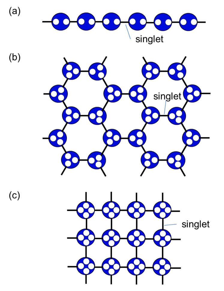
Figure 1: The Valence Bond Solid (VBS) is constructed by allocating on each site as many spin-1/2 particles (in their symmetric subspace) as neighboring sites, e.g., (a) 2 for 1D chains, (b) 3 for the hexagonal lattice, and (c) 4 in the 2D square lattice. For each pair of neighboring sites, the VBS state places a singlet between two spin-1/2. Having a singlet connecting sites imposes restrictions on the total spin evaluated on neighboring sites by $P^{(S=s_{\max})}$.

Let us briefly explain why the AKLT Hamiltonians are spin rotation invariant. Consider the spin-1 chain. Let $\vec{S}_{ij}\equiv\vec{S}_{i}+\vec{S}_{j}$. Then projection of sites $i$ and $j$ to their joint spin-2 subspace is given by $P=\lambda[S_{ij}^{2}-0][S_{ij}^{2}-1(1+1)]$, as it annihilates states in $S_{ij}=0,1$ subspaces. The coefficient $\lambda$ is determined by the requirement that $P$ is a projection on the $S_{ij}=2$ subspace, i.e., $P|S_{ij}=2,S_{z}\rangle=|S_{ij}=2,S_{z}\rangle$, which leads to $1/\lambda=[2(2+1)-0][2(2+1)-1(1+1)]=12$. Then by expanding $S_{ij}^{2}=S_{i}^{2}+S_{j}^{2}+2\vec{S}_{i}\cdot\vec{S}_{j}$ and using that $S_{i}^{2}$ and $S_{j}^{2}$ are constants (2 for spin 1) we obtain that the Hamiltonian contains a polynomial of $\vec{S}_{i}\cdot\vec{S}_{j}$ up to degree 2 (and $s_{\max}$ in general). The resultant AKLT Hamitonians for the spin-1 chain, the spin-3/2 honeycomb lattice, and the spin-2 square lattice are shown in Eqs. (3), (7), and (8), respectively. Thus we arrive at the conclusion that the AKLT Hamiltonian is spin rotation invariant and, additionally, semidefinite positive. Its ground state, the AKLT wavefunction, has energy $E_{0}=0$. This ground state –the VBS– has also total angular momentum $S^{\rm tot}=0$ and $z$ component $S^{\rm tot}_{z}=0$. The AKLT Hamiltonian commutes with $(S^{\rm tot})^{2}$ (where $\vec{S}^{\rm tot}\equiv\sum_{i}\vec{S}^{(i)}$) and $S^{\rm tot}_{z}\equiv\sum_{i}S^{(i)}_{z}$, thus they are good quantum numbers and the eigenstates of the AKLT (or any such spin-rotation invariant) Hamiltonian can be labeled by $|S^{\rm tot},S^{\rm tot}_{z},\alpha\rangle$, where $\alpha$ is some additional labeling for different ways of constructing $|S^{\rm tot},S^{\rm tot}_{z}\rangle$ states. Furthermore, for a given $S^{\rm tot}$ and $\alpha$, the different sublevels characterized by $S^{\rm tot}_{z}$ are degenerate.

We show here how the conservation of the angular momenta can be utilized to compute the gap (even in the thermodynamic limit), by adding a local field term $h\,S^{\rm tot}_{z}$ to the Hamiltonian. We shall consider the total Hamiltonian

$$H(h)=H_{\rm AKLT}+h\sum_{i}S^{(i)}_{z}.$$ (2)

Because of $[S^{\rm tot}_{z},H_{\rm AKLT}]=0$, the VBS ground state does not interact with the local field and has ground state energy remaining zero for any value of $h$. For $h>0$, any excited state with $S_{z}\neq 0$ interacts with the local field and the corresponding zero-field degenerate levels split linearly with $S_{z}$. Here we assume that spin triplets are elementary excitations, as will be justified later. If there is a gap, for some field value $h_{t}>0$ the energy of some level will cross the zero energy to negative, becoming the ground state of the system at the field $h_{t}$. We can observe this transition by computing the energy or the z-component total angular momentum $S_{z}^{\rm tot}$ of the ground state and detecting the transition to $S_{z}\neq 0$ (nonzero magnetization). Interestingly, this can be computed efficiently in the TN description.

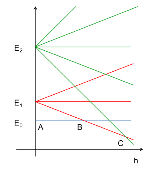
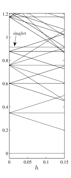
Figure 2: Left: A schematic picture for the level splitting under the external field $h$ for a generic antiferromagnetic spin-rotation invariant Hamiltonian. A represents the location of the ground-state energy at the zero field. The crossings at B, C, etc., represent the ground state switching to one with a different set of quantum numbers. In the thermodynamic limit, the envelope curve for the $E_{0}$ plateau (if it exists) and the successive crossings form the ground state energy curve for the system in presence of the external field $h$. Knowing the first crossing and the slope, one can extrapolate to obtain the zero-field spectral gap. If the first crossing is by the one with a slope $-1$, then the value of $h$ at the crossing point gives the spectral gap. One is interested in the gap in the thermodynamic limit, i.e., the property of this crossing in such limit. Right: The actual spectrum of a $N=8$ AKLT chain with external field (Eq.2). Notice the presence of singlets as excitations at high energies.

As shown schematically in Fig. 2, the response of the non-zero angular momentum states is linear with the field, so from the slope in the energy curve for $h>h_{t}$ we can determine (by linear extrapolation) the energy of each state at $h=0$. As for the gap, we are interested in the first excited state(s). It might be possible that as the field is increased such states never appear as the ground state (of the field-dependent Hamiltonian), as they may be (i) insensitive to the field, i.e., they are also states characterized by $S^{\rm tot}=S^{\rm tot}_{z}=0$, or (ii) before they cross the zero energy curve, higher energy states already cross the zero. We shall argue and provide evidence from exact diagonalization on small systems that (i) the first excited states of antiferromagnetic Hamiltonians (such as Heisenberg and AKLT) are never characterized by $S^{\rm tot}=S^{\rm tot}_{z}=0$ but by $S^{\rm tot}=1,S^{\rm tot}_{z}=\pm 1,0$. If case (ii) occurs, then the determination of the gap from our method will turn into a set of lower bounds. However, we shall also show numerical evidence that (ii) does not occur in our consideration. Moreover, analysis from field-theory treatment on the spin-1 Heisenberg chain predicts that triplets are indeed the lowest excitations affleckPRB . An important part of this work is dedicated to show that the identified transition shows the exact value of the gap.

In this work we utilize various numerical methods, from exact diagonalization and 1D Matrix Product States (MPS) variation method and iTEBD, to the 2D Tensor Network Renormalization Group (TNRG). These methods have nowadays become standard tools to obtain phyical properties in the thermodynamic limit. In the following, we only mention essence of these methods and we refer the readers to the literature for detailed implementation.

We compute the gap of the AKLT Hamiltonian in 1D for finite chains of increasing length, and we directly study as well the infinite case by means of MPS techniques. The resulting gap value $\Delta\cong 0.350$ agrees with previous bounds, but under the above-mentioned assumptions our value is a direct estimation of the gap. We apply the same ideas to the spin-3/2 hexagonal lattice, and find a gap $\Delta\cong 0.101$ using infinite-size Tensor Network methods. Our value is in excellent agreement with previous results obtained by exact diagonalization over small clustersganesh of $N=12-18$ spins. We also obtain a value of the gap $\Delta\cong 0.03$ for the spin-2 square lattice. Notice that all these gap values are obtained from the AKLT Hamiltonian formulated to be the sum of projectors (see Eq.3, 7 and 8), with a coupling term $J<1$ that rescales the energy spectrum, compared to the corresponding Heisenberg Hamtiltonians.

We organize this paper showing first exact results for the 1D spin-1 AKLT model in Section II. We apply MPS techniques to compute the gap in the thermodynamic limit in Section III, where we check our method gainst DMRG results for the spin-1 Heisenberg chain. Then we show how similar techniques can be used for the computation of the gap in 2D systems: in Section IV we show results for the hexagonal spin-3/2 lattice, and in Section V we compute the gap of the square spin-2 lattice. Finally, conclusions are presented in Setion VI.

II 1D AKLT Hamiltonian

In this section we put onto solid grounds and elaborate the ideas presented in the introduction by running some exact calculations for small 1D systems. We explore the energy spectrum around $h=0$ for the total Hamiltonian in Eq. (2) where for spin-1 systems we have

$$H^{S=1}_{\rm AKLT}=\frac{1}{2}\sum_{\langle i,j\rangle}\left[{\vec{S}_{i}\cdot\vec{S}_{j}}+\frac{1}{3}(\vec{S}_{i}\cdot\vec{S}_{j})^{2}+\frac{2}{3}\right]$$ (3)

We note that due to the requirement of being a projector for nearest-neighbor interaction, there is a factor $J=1/2$ compared to the usual Heisenberg Hamiltonian with $J=1$. In order to ensure the uniqueness of the ground state in finite calculations we impose periodic boundary conditions.

We compute the energy of the $6$ lowest energy states for different values of $h$ and evaluate $S_{z}^{tot}$ for the ground state. In Fig.3 we plot these values for a system of $N=12$ as an illustration. In the upper panel we plot the energy per particle of each energy level, and the lower panel shows $S_{z}^{tot}$ of the ground state. At $h=0$ we observe a ground state with $E_{0}=0$ –the AKLT state– and a gap with the first excited state with a triple degeneracy and $S_{z}^{tot}=-1,0,1$. The fact that the energy splits into three levels linearly with the field shows that they have $S_{\rm tot}=1$. Of these 3 lowest-energy excited states, one with $S_{z}^{\rm tot}=-1$ interacts with the field $h>0$ linearly with slope $S_{z}^{\rm tot}=-1$. At a given value of $h_{t}=\Delta$ this excited state has energy $E_{1}=0$, and becomes the ground state for $h>h_{t}$. Other higher levels will come down and cross this level for larger $h$. The original ground state, having $S_{z}^{\rm tot}=0$ keeps having $E_{0}=0$ for any finite $h$. In this scenario there are two ways to extract the gap. First, we can extrapolate from the value of $h=h_{t}$ back linearly to $h=0$ and locate the cross point with the y-axis. Second, without extrapolation, this value of the field $h_{t}$ provides a direct reading of the exact value of the energy gap. (This second view will be useful in the thermodynamic limit, where one has only access to energy and magnetic moment per site). The transition to a ground state with $S_{z}^{tot}=-1$ is just the first of a series of successive transitions to ground states with increasing $S_{z}^{tot}$ which appear after the crossing of the current ground state with excited states with higher $S^{tot}$ –and thus a steepest slope in the energy spectrum. Moreover, for each value of $h$, $S_{z}^{tot}$ is the derivative of the energy and we can observe the transition from these two magnitudes.

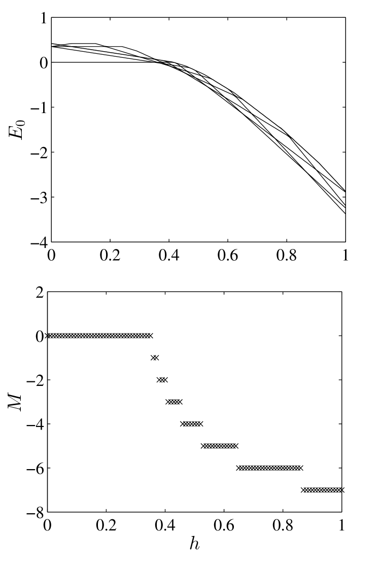
Figure 3: For the Hamiltonian Eq.2 we plot the energy per particle (top) of the $6$ eigenstates with lower energy, and $S_{z}^{tot}$ of the ground state (bottom) as a function of the field $h$, with system size $N=12$ and PBC. At $h=0$ we observe a gap $\Delta$ between the ground state and the triple-degenerate first excited state. Of these 3 sates, one crosses the ground state at $h=\Delta$ after interacting linearly with the field. At this point, the ground states makes a transition to $S_{z}^{tot}=-1$. Successive crossings of higher $S_{z}^{tot}$ will further decrease the total $S_{z}^{tot}$ of the ground state an they become the new low energy states, up to a total $S_{z}^{tot}=Ns$.

	AKLT		Heisenberg
N	$E_{1}-E_{0}$	$E_{2}-E_{0}$	$E_{1}-E_{0}$
8	0.349849122	0.4988577	0.5935552
10	0.350091873	0.4477184	0.5248079
12	0.350120437	0.4187836	0.4841964
14	0.350123733	0.4009563	0.4589653
16	0.350124109	0.3892351	0.4427955

Table 1: Exact gap calculation for spin chains in periodic boundary conditions with increasing length $N$. We show also the energy gap to the second excitation.

Our exact results for different values of $N$ are shown in Table 1, including similar calcuations for the Heisenberg model. Unlike this latter case, in the AKLT we observe a growing energy gap for longer systems, converging to a value $\Delta=0.350$. This is in agreement with previous upper boundsKnabe ; Auerbach . The second transition converges to $\Delta_{2}=\Delta$, which suggests that even in the thermodynamic limit the first transition to a $S_{z}^{tot}\neq 0$ ground state will take place to a state with $S_{z}^{tot}=1$. As shown in Fig.4 the gap for the AKLT has a clear $\frac{1}{N}$ dependence. We will complete this result in the following sections with direct numerical calculations in the thermodynamic limit using Tensor Network methods, but this finite size scaling suggests that our readings of the transition in the ground state at $h_{t}$ provide a direct measurement of the gap.

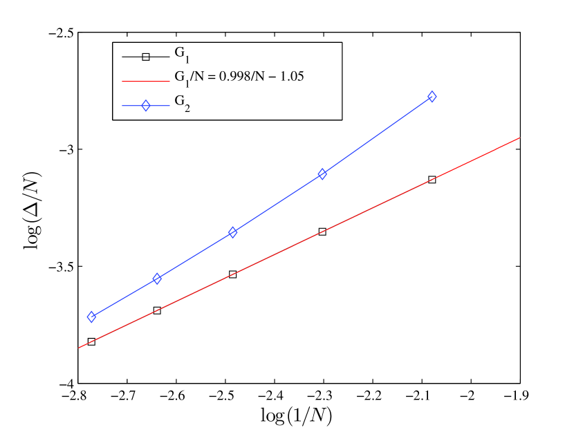
Figure 4: From the exact diagonalization we extract estimations of the gap in the thermodynamic limit of the AKLT Hamiltonian. Left: The energy gap per site $\Delta/N$ vs. $\frac{1}{N}$ for $N=8,10,12,14,16$. The slope of this plot, wtih a good linear fitting, provides the gap estimation $\Delta=0.350$. We plot in blue the difference between the gap to the first excitation and to the second excitation $(E_{2}-E_{1})/N$ vs. $\frac{1}{N}$ for $N=8,10,12,14,16$. With a good square fitting, we observe at $\frac{1}{N}\rightarrow 0$ we a small but positive value of $(E_{2}-E_{1})/N$, so we expect that the first transition to $S_{z}=-1$ is robust in the thermodynamic limit.

III MPS calculations of finite and infinite 1D systems

The exact results in Section II confirm the picture described in Section I, and show how one can extract the value of the gap from the magnetization of ground states. Unfortunately by exact diagonalization, this can be computed for only a few particles. We complete these calculations by showing results computed using tensor network techniques in 1D systems. The following sections will present results for 2D lattices.

MPS and tensor networks provide a detailed description of ground states of local Hamiltonians, and are efficient methods for systems with an energy gap. This implies that for the gapped phase we are exploring here, we can obtain good approximations to the ground state at $h=0$ if there is a gap in the AKLT model. However, we have seen that this gap closes for higher $h$, and then follows a succession of transitions to new ground states. The region near the first transition represents a region close to a continuous quantum phase transition. This translates into a not-so-efficient description of the ground state in this region, so we expect the need of higher bond dimension $\chi$ for the ground state representation. Nevertheless, a good estimationof the phase transition point can be identified by suitable scaling analysis scaling .

Even though we can complete the finite size calculations using finite MPS to obtain the gap for larger systems, due to the fast convergence of this transition value for short chains this task brings little additional information. Moreover, the precision required to assess the $\frac{1}{N}$ dependence found above is numerically demanding. This requires i.e. $\chi=20$ for size $N=12$, in order to obtain the transition for a value of $h$ compatible with the exact diagonalization. Lower values of $D$ will place this transition at higher $h$, which exemplifies the need for relatively high $\chi$ values even for small chains, due to the critical character of the transition.

We can access directly by means of the iTEBD algorithm a representation of the infinite chain by imposing translational invariance in the tensor description (for details see Vidal07 ). The final process however will produce energy and magnetic moment per particle, as opposed to the total energy and total magnetic moment of the exact diagonalization and MPS for finite systems. This means that we cannot extrapolate the energy from the transition point back to $h=0$ to obtain the vertical offset as the energy gap. However, using the second viewpoint mentioned earlier, the field value at which the energy density and the magnetization becomes negative is the value of the energy gap, and no extrapolation is necessary.

We show the iTEBD results for the energy per site in Fig.5, where we can observe clearly a plateau up to $h\sim 0.35$, indicating the gapped phase. This result resembles those in Fig.3 for $N=12$, due to the fast convergence of the spectrum. The solid line in Fig.6 shows $M=S_{z}$ per site in the thermodynamic limit as computed using $\chi=60$ iTEBD. The energy curve displays a plateau followed by a transition at $h=0.350$. The points in Fig.6 are results for $N=10$ obtained by exact diagonalization, displayed here as a reference. For an accurate estimation of the transition, we study the scaling $S_{z}\sim(h-h_{c})^{\beta}$ to obtain $\Delta=0.350$. These results are computed using $\chi=60$ and shown in the inset of Fig.6.

At this point it is interesting to consider the limiting cases we have already explored. Observing the magnetization curves, new plateaus of the magnetization appear for increasing $N$ corresponding to the new values available to the magnetization from the new spin combinations. However, the gap and the value of the field for the totally polarized state are similar for different sizes. This restricts the existing and new plateaus of the magnetization into a the same range of field values. Progressively with increasing $N$ the plateaus will shorten their width, and in the limit $N\rightarrow\infty$ the plateaus will appear at any value of $S_{z}$ (per particle) with an infinitesimal width. This is clearly depicted in Fig.6. The transition point –as read from the magnetization– agrees with the value $\Delta=0.350$ obtained from the finite size scaling.

We comment on an interesting observation. The last plateau where the spins become completely polarized $|-1,-1,-1,...\rangle$ begins at $h=2$. This is due to a transition from a previous plateau characterized by a state of the form

$$|\psi\rangle=\frac{1}{\sqrt{N}}\sum_{j=1}^{N}(-1)^{j}|-1\rangle|-1\rangle...|-1\rangle_{j-1}|0\rangle_{j}|-1\rangle_{j+1}...|-1\rangle.$$ (4)

By direct calculation, we can show that this is an eigenstate and has energy $(N-2)-h(N-1)$. Comparing with the completely polarized state, which has energy $N-hN$, we find that the crossing occurs at the $h=2$. As we shall see in the two dimensional case, the same type of states give the last crossing at $h=3$ in the honeycomb and $h=4$ in the square lattice case (in general $h=z$, the number of neighbors).

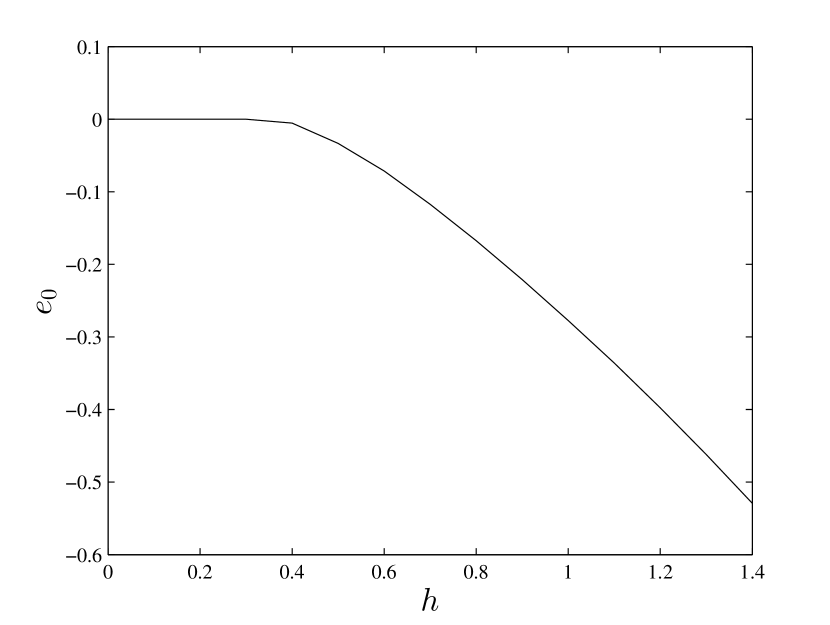
Figure 5: Ground state energy per site of the AKLT Hamiltonian for an infinite chain as computed using iTEBD with $\chi=30$. We can identify a plateau around $h=0$, and the transition to $e_{0}<0$ indicates a change in the ground state. The value $h_{c}$ is used to obtain the gap $\Delta$.

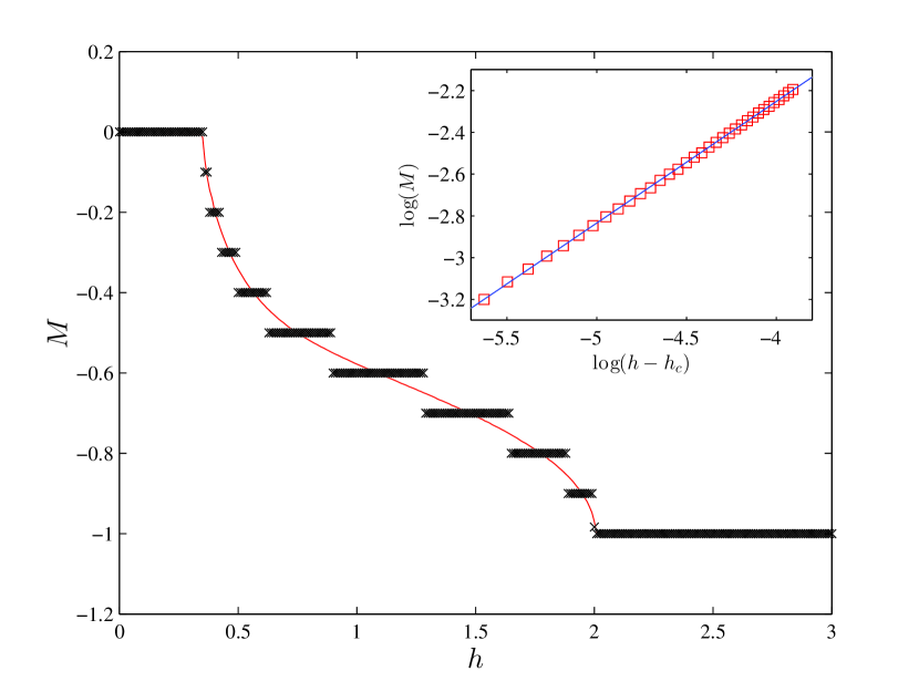
Figure 6: $S_{z}$ per site of the AKLT Hamiltonian for an infinite chain as computed using iTEBD with $\chi=30$ (red solid line). The exact results for $N=10$ are shown in black crosses as a reference. Inset: With a scaling fit of $S_{z}$ close to the transition, we obtain a value of the transition $\Delta=0.350$. A bigger bond dimension $\chi=60$ is used to perform this fit.

The existence of a finite nonzero gap in the thermodynamic limit was already established by AKLT AKLT2 via lower bounds and their technique was subsequently generalized by Knabe Knabe and by Nachtergaele Nachtergaele . However, the lower bounds provided by these methods are not tight. Our method for accessing the gap via the external field $h=\Delta$ holds even for $N\rightarrow\infty$ whenever the first excited state – which is a triplet– has total $S_{z}=-1$ (as the system approaches infinityaffleckPRB2 ). In this direction is important to study the structure for the first excited state. In Knabe the elementary excitations (so-called crackions) are expressed as a variational perturbation over the AKLT state, by the superposition of states formed by breaking one of the virtual singlet bonds. These excitations in fact are not eigenstates of the Hamiltonian in Eq. 3 but provide an upper bound of the energy of the first excited state. This value $\Delta=\frac{10}{27}\cong 0.37$ can also be derived from the single-mode approximation Auerbach and is close to but higher than our estimation $\Delta=0.350$.

From the proposed excited states we also discard the existence of other states with $S^{tot}=0$ between the ground state and the first excitations with $S^{tot}=1$. These excitations don’t interact with the field $h$ and thus will never cross the ground state, making them invisible to our method. However, field-theory argumentsaffleckPRB and numerical results whiteGap ; HeisGap indicate that the first excitation is a triplet with $S^{tot}=1$, and the first excitation with $S^{tot}=0$ appears with very high energy. This is consistent with our finite size results of Table 1 and Fig. 4.

III.1 1D Bilinear biquadratic Model

The AKLT model is a particular case of the family of the bilinear biquadratic Hamiltonian written as

$$H_{BB}=\sum_{\langle i,j\rangle}\left[\vec{S}_{i}\cdot\vec{S}_{j}+\gamma(\vec{S}_{i}\cdot\vec{S}_{j})^{2}\right].$$ (5)

We note that the AKLT model corresponds to $\gamma=1/3$. However, in order to write the AKLT as a composition of projecting operators one includes an overall factor $J=1/2$ (see Eq. (3) as the Hamiltonian used earlier).

As a direct extension of the previous analysis of the AKLT model we use the same techniques to explore the gap of Eq. 5 for the Heisenberg model, i.e. the case with $\gamma=0$. Previous DMRG calculations show accurately a gapped phase with $\Delta=0.4107$ whiteGap , and bounds to this gap have been calculated in HeisGap . In Ref.affleckPRL a bosonic model for the excitations of the Hesenberg model provides a scaling function around the transition to $e_{0}<0$ as

$$M\sim\frac{\sqrt{(h-h_{c})\Delta}}{2v\pi},$$ (6)

where $\Delta$ is the energy gap and $v$ the magnon velocity.

Using the method presented above we compute the gap and magnon velocity using a fit of $S_{z}$ around $h_{c}$, which also provides the value of the gap $\Delta$. Our results are shown in Fig.7. These results are obtained with iTEBD and $\chi=80$ with fourth order Trotter evolution for the state preparation. From the fit (see the inset of Fig.7) we obtain $\Delta=0.4105$ and $v=2.37$, in good agreement with the results in affleckPRL ; WeyrauchRakov and the DMRG result in whiteGap .

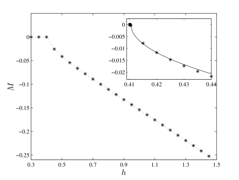
Figure 7: For the Heisenberg spin-1 model, the transition in the magnetization $M$ vs. the field $h$. Excitations are states of $S_{z}^{tot}=-1$, and we read directly the gap from the transition in the ground state magnetization $S_{z}^{tot}\neq 0$. The dotted line is included as a reference, not actual data. Inset: Detailed view of the transition region. The solid line is a fit to the function $M\sim\frac{\sqrt{(h-h_{c})\Delta}}{2v\pi}$. From the fit we obtain $\Delta=0.4105$ and $v=2.37$.

IV Hexagonal lattice in 2D

Using PBC, the spin-3/2 AKLT state, e.g, on the honeycomb lattice is the unique ground state of the following Hamiltonian with spin rotational symmetry

$$H^{S=3/2}_{\rm AKLT} = \frac{27}{160}\sum_{\langle i,j\rangle}\Big{[}\vec{S}_{i}\cdot\vec{S}_{j}+\frac{116}{243}(\vec{S}_{i}\cdot\vec{S}_{j})^{2}$$ (7)

$$+\frac{16}{243}(\vec{S}_{i}\cdot\vec{S}_{j})^{3}+\frac{55}{108}\Big{]},$$

defined on trivalent lattices AKLT2 . If open boundary conditions are used or the boundary spin-3/2’s are terminated by spin-1/2’s with Heisenberg-type interaction (between the spin-1/2 and the boundary spin-3/2) the ground state is unique. Similarly, AKLT states defined on any tetravalent lattice, such as the square, Kagomé and the 3D diamond lattices, are the ground states of a spin isotropic Hamiltonian with the highest order term proportional to $(\vec{S}_{i}\cdot\vec{S}_{j})^{4}$.

In order to study this lattice in the thermodynamic limit we use the TNRGlevin ; wen ; xiangPRB method to obtain expectation values of the energy and magnetization per site. This method is governed by a parameter $D$ for the state preparation by local update, and $D_{cut}$ for the RG calculation. Obtaining values for finite systems with TN requires either setting PBC or including boundary spin-1/2 particles to obtain a unique ground state. These two approaches are more involved than TNRG, and we are mainly interested in proving propertied of the infinite lattice. For exact calculations in finite systems, we impose PBC in our numerics.

The approach to 2D systems presented here is the same as for the 1D spin chain. In the infinite limit we have only access to expectation values per site, which is enough to identify the transition between the ground state and excited states at some $h$, as will be shown. Scanning for different values of $h$ and computing the energy and magnetization, we identify the transition at which they first become negative, i.e., $e_{0}<0$ and $m_{z}<0$.

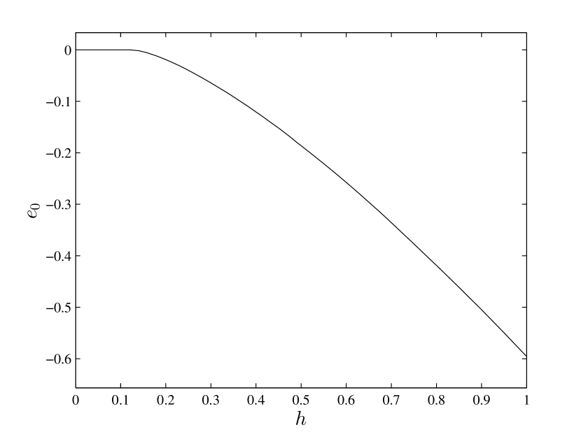
Figure 8: Ground state energy per site $e_{0}$ as a function of the field $h$, computed with $D=3$ and $D_{cut}=20$. We observe a flat region around $h=0$ indicating the presence of a gap $\Delta$. The transition to $e_{0}<0$ at $h_{c}$ provides a direct reading of a lower bound to the gap.

We plot the results of this procedure to obtain the energy per site in Fig.8 using $D=3$ for the ground state tensors, and $D_{cut}=20$ for the RG method. We clearly observe a plateau of $e_{0}=0$ up to the value $h_{c}\sim 0.1$. A more accurate analysis is presented for the magnetization $S_{z}$ per site in Fig.9. We again observe a flat region before the transition at $h_{c}\sim 0.1$, indicating the presence of an energy gap. These results are in good agreement with finite size calculations sylvain ; ganesh over small clusters of spins. The inset shows results around the transition point using $D=2,3,4,5$ for the ground state tensors, and $D_{cut}=20$ for the RG method. As a remark, we observe the transition to the fully polarized state of the hexagonal lattice at a value of the field $h_{f}=3$. As explained above, this transition happens at $h_{f}=2s$ (with $s$ the local spin).

We compare the TNRG results with exact diagonalization for small lattices as a reference. We construct a small lattice with PBC of size $2\times 4$ and $3\times 4$ to obtain the gap (see Fig. 10). For these settings we obtain the gap values $\Delta_{2\times 4}=0.092029$ and $\Delta_{3\times 4}=0.095345$. Notice that again the first transition provides an exact reading of the gap: this suggests that for small systems the single spin excitations are the lowest excited states, as in the 1D chain. However, without bounds for the excitation energy in the infinite hexagonal lattice, we can only conjecture that the transition values coincide with the gap in the thermodynamic limit, i.e. the elementary excitations have $S^{tot}=1$.

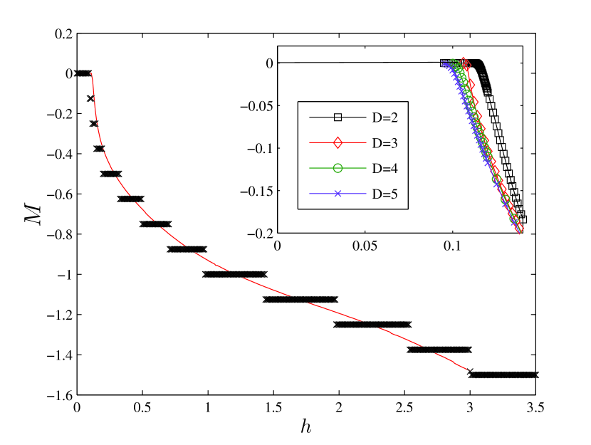
Figure 9: $S_{z}$ per site of the AKLT Hamiltonian for an infinite hexagonal lattice as computed using TNRG with $D=3$ and $D_{cut}=20$ (red solid line). The cross marks are exact results for a lattice $2\times 4$ using PBC. Inset: Transition in the magnetization of the infinite hexagonal lattice using $D=2,3,4,5$ using $D_{cut}=20$.

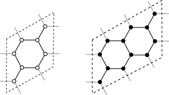
Figure 10: Disposition of the lattices used for finite size calculations of the finite hexagonal lattice with PBC to compute the gap by exact diagonalization. For a lattice (white circles, left) we find $\Delta_{2\times 4}=0.092029$. Introducting $4$ additional sites (to the right in black circles, with a total size $3\times 4$) we obtain $\Delta_{3\times 4}=0.095345$.

As shown in the inset of Fig. 9 the transition point shifts to lower values of $h_{c}$ as the bond dimension $D$ increases. Exact diagonalization results suggest –as in 1D chains– higher values of the gap for larger systems. Identifying a critical transition using Tensor Network methods requires large bond dimensions and a careful choice of the interval for the scaling fitsandvik .

To identify the infinite-system transition point from our results using TNRG (see the inset in Fig.9), we perform a scaling analysis for different values of $D$. We use the scaling relation for the magnetization close to the transition point $M\sim(h-h_{c})^{\beta}$. Fitting the energy, we obtain $h_{c}={0.12,0.108,0.104,0.100}$ for $D=2,3,4,5$ respectively. Using the magnetization in a similar way we obtain $h_{c}={0.12,0.108,0.105,0.101}$. The fitting results for the magnetization $S_{z}$ are shown in Fig.11.

Figure 11: Using the scaling relation $M\sim(h-h_{c})^{\beta}$ we obtain the value of the critical transition for $D=2,3,4,5$ at $h_{c}=0.12,0.108,0.105,0.101$ respectively. Using the energy instead of the magnetization (not shown here), we obtain similar transition values.

V Square lattice in 2D: infinite study with TNRG

We finally study the 2D square lattice, where the AKLT state can be viewed as 4 spin-1/2 particles at each site, for a total local spin $s=2$. The AKLT hamiltonian projects two neighboring $s=2$ particles into the spin $s=4$ subspace, resulting in the Hamiltonian

$$H^{S=2}_{\rm AKLT} = \frac{1}{14}\sum_{\langle i,j\rangle}\Big{[}\vec{S}_{i}\cdot\vec{S}_{j}+\frac{7}{10}(\vec{S}_{i}\cdot\vec{S}_{j})^{2}$$ (8)

$$+\frac{7}{45}(\vec{S}_{i}\cdot\vec{S}_{j})^{3}+\frac{1}{90}(\vec{S}_{i}\cdot\vec{S}_{j})^{4}\Big{]}.$$

Following the same procedure as for the spin-1 and spin-3/2 AKLT systems, we compute the transition $h_{c}$ from the magnetization $S_{z}$. Our results are obtained solely using TNRG in the infinite limit, and are shown in Fig. 12 for $D=2,3$. Even though the plateau cannot be clearly observed as in the other models, a scaling fit of the magnetization (see the inset in Fig. 12) is compatible with a gap value $\Delta=0.03$. Such a small value has to be considered together with the prefactor $J=\frac{1}{14}$ so the Hamiltonian is formed as a combination of projecting operators.

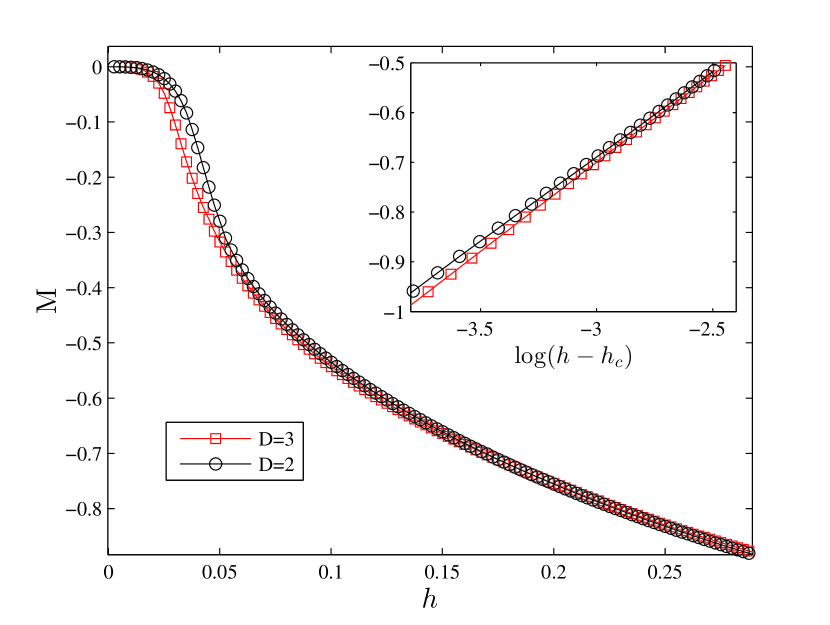
Figure 12: Magnetization curve for the spin-2 AKLT Hamiltonian in presence on an external field $h$ on the square lattice. We show here results for $D=2,3$ simulations using TNRG where we set $D_{cut}=20$. Inset: Using the scaling reation $M\sim(h-h_{c})^{\beta}$ we plot $\log(h-h_{c})$ vs. $\log(M)$, from where we obtain a transition at $h_{c}=0.03$.

VI Conclusions

The study of the gap of AKLT Hamiltonians conducted here starts with exact diagonalization for finite systems that suggest the existence of a gapped phase and provides evidence supporting that the first excited states form a triplet. For 1D spin-1 chains we have both lower and upper bounds for this gap, which agree with our finite size scaling results. Using MPS we can access longer systems sizes, but the gap is clearly observed to converge quickly even at small chain lengths. We complete the picture in 1D with iTEBD results that also agree with the finite size results, resulting in a gap for the spin-1 AKLT chain of $\Delta\cong 0.350$.

In 2D, numerical exact results reach only hexagonal lattices of small size. Finite size PEPS simulations may complement these results for a proper finite size scaling; however, we did do this. Instead, using TNRG techniques we directly access the thermodynamic limit and obtain a value of the gap $\Delta\cong 0.10$ in agreement with the finite results. This agreement arises from two observations: the gap increases with the system size, and the fast convergence of the gap with $N$ can be observed even in very small systems. For the square lattice we cannot obtain exact results for appropriate sizes and we rely solely on TNRG results. These results suggest also a gapped phase with $\Delta\cong 0.03$.

Our method to compute the gap in the limit of infinite system size introduces an additional field term in the Hamiltonian commuting with it and this is equivalent to probing the first quantum phase transition as $h$ increases from $0$. We have shown results for the AKLT Hamiltonian, and in general for the bilinear biquadratic model in the gapped phase. Our results have good agreement with previous bounds and DMRG result for 1D spin chains. Nevertheless, the general idea of this method can be applied by identifying symmetries in ground states of Hamiltonians commuting with the additional external field. It would be desirable to have analytic proof for the existence of the gap.

Note added: Similar results on the honeycomb lattice were recently obtained in psc .

- (1) F. D. M. Haldane, Phys. Lett. A 93, 464 (1983).
- (2) F. D. M. Haldane, Phys. Rev. Lett. 50, 1153 (1983).
- (3) E. H. Lieb, T. D. Schultz, and D. C. Mattis, Ann. Phys. (N.Y.) 16, 407 (1961).
- (4) I. Affleck, T. Kennedy, E. H. Lieb, and H. Tasaki, Comm. Math. Phys. 115, 477 (1998).
- (5) M. Fannes, B. Nachtergaele, and R. F. Werner, Comm. Math. Phys. 144, 443 (1992).
- (6) S. Knabe, J. Stat. Phys. 52, 627 (1988).
- (7) B. Nachtergaele, Comm. Math. Phys. 175, 565 (1996).
- (8) M. Hastings and T. Koma, Comm. Math. Phys. 265, 781 (2006).
- (9) B. Nachtergaele and R. Sims, Comm. Math. Phys. 265, 119 (2006).
- (10) R. Ganesh, D. N. Sheng, Young-June Kim and A. Paramekanti1, Phys. Rev. B 83, 144414 (2011).
- (11) R. Raussendorf and H. J. Briegel, Phys. Rev. Lett. 86, 5188 (2001).
- (12) H. J. Briegel, D. E. Browne, W. Dür, R. Raussendorf, and M. Van den Nest, Nature Phys. 5, 19 (2009).
- (13) R. Raussendorf and T.-C. Wei, Annual Review of Condensed Matter Physics 3, pp.239-261 (2012).
- (14) D. Gross and J. Eisert, Phys. Rev. Lett. 98, 220503 (2007).
- (15) G. K. Brennen and A. Miyake, Phys. Rev. Lett. 101, 010502 (2008).
- (16) T.-C. Wei, I. Affleck, and R. Raussendorf, Phys. Rev. Lett. 106, 070501 (2011).
- (17) A. Miyake, Ann. Phys. (Leipzig) 326, 1656 (2011).
- (18) T.-C. Wei, I. Affleck, and R. Raussendorf, Phys. Rev. A 86, 032328 (2012).
- (19) M. A. Nielsen, Rep. Math. Phys. 57, 147 (2006).
- (20) I. Affleck, T. Kennedy, E. H. Lieb, and H. Tasaki, Phys. Rev. Lett. 59, 799 (1987).
- (21) T. Kennedy, E. H. Lieb, and H. Tasaki, Journal of Stat. Phys. 53, 383 (1988).
- (22) Ian Affleck, Phys. Rev. B 41, 6697 (1990).
- (23) A. Auerbach, Interacting Electrons and Quantum Magnetism (Springer-Verlag, New York, 1998).
- (24) L. Tagliacozzo, T. R. de Oliveira, S. Iblisdir, J. I. Latorre, Phys. Rev. B 78, 024410 (2008).
- (25) G. Vidal, Phys. Rev. Lett. 98, 070201 (2007).
- (26) Ian Affleck, Phys. Rev. B 43, 3215 (1991).
- (27) S.R. White and D. A. Huse, Phys. Rev. B 48, 3844-3852 (1993).
- (28) D. P. Arovas, A. Auerbach and F. D. M. Haldane, Phys. Rev. Lett. 60, 531 (1988).
- (29) E. K. Sorensen and I. Affleck, Phys. Rev. Lett 71, 1633 (1993).
- (30) M. Weyrauch and M. V. Rakov, Ukr. J. Phys. 58, 657 (2013).
- (31) M. Levin and C. P. Nave, Phys. Rev. Lett. 99, 120601 (2007).
- (32) Z. C. Gu, M. Levin and X. G. Wen, Phys. Rev. B 78, 205116 (2008).
- (33) H. H. Zhao, Z. Y. Xie, Q. N. Chen, Z. C. Wei, J. W. Cai and T. Xiang, Phys. Rev. B 81, 174411 (2010).
- (34) S. Capponi, private communication.
- (35) Chen Liu, Ling Wang, Anders W. Sandvik, Yu-Cheng Su, Ying-Jer Kao, Phys. Rev. B 82, 060410(R) (2010).
- (36) D. Poilblanc, N. Schuch, J. I. Cirac, arXiv:1308.3463 (2013).