Thermodynamics of QCD at vanishing density

Abstract

We study the phase structure of QCD at finite temperature within a Polyakov-loop extended quark-meson model. Such a model describes the chiral as well as the confinement-deconfinement dynamics. In the present investigation, based on the approach and results put forward in Braun et al. (2011); Herbst et al. (2013); Haas et al. (2013); Mitter and Schaefer (2013), both, matter as well as glue fluctuations are included. We present results for the order parameters as well as some thermodynamic observables and find very good agreement with recent results from lattice QCD.

I Introduction

The study of strongly interacting matter under extreme conditions is a very active field of research. Experiments conducted at CERN, RHIC and the future FAIR and NICA facilities aim at probing the phase structure of Quantum Chromodynamics (QCD).

From the theoretical side, calculating the phase structure from first principles is a hard task which requires the use of non-perturbative methods. Over the recent years a lot of progress has been made in this direction. In particular it has been shown that, apart from lattice QCD, also continuum methods, such as the Functional Renormalisation Group (FRG) Litim and Pawlowski (1999); Berges et al. (2002); Pawlowski (2007); Gies (2012); Schaefer and Wambach (2008); Pawlowski (2011); Braun (2012); von Smekal (2012) are well suited to study the QCD phase diagram. This has been demonstrated in e.g. Braun et al. (2010a, 2011); Fischer and Luecker (2013); Fister and Pawlowski (2013); Fischer et al. (2013); Haas et al. (2013) at vanishing as well as finite temperature and chemical potential. Complementary to first-principles studies, low-energy QCD has been studied successfully within effective models. Especially the use of Polyakov-loop extended chiral models makes it possible to study the interrelation of the chiral and deconfinement phase transitions, e.g. Meisinger and Ogilvie (1996); Pisarski (2000); Fukushima (2004); Megias et al. (2006); Ratti et al. (2006); Mukherjee et al. (2007); Roessner et al. (2007); Sasaki et al. (2007); Schaefer et al. (2007); Fraga and Mocsy (2007); Fukushima (2008); Sakai et al. (2008); Herbst et al. (2011); Skokov et al. (2011, 2010a); Schaefer and Wagner (2012); Braun and Janot (2011); Kamikado et al. (2013); Braun and Herbst (2012); Fukushima and Kashiwa (2013); Mintz et al. (2013); Herbst et al. (2013); Haas et al. (2013); Stiele et al. (2013); Strodthoff and von Smekal (2013). However, the confinement sector in these models is not fully constrained, resulting in various parametrisations of the corresponding order-parameter potential, the glue or Polyakov-loop potential. Furthermore, the important unquenching effects on the glue potential are usually not included. Ideally, this potential is derived from QCD directly, leaving no ambiguity. This has recently been accomplished with the FRG for two-flavour QCD in the chiral limit Braun et al. (2011) and for $2+1$ flavours in Fischer et al. (2013) and puts us in the position to make use of these results to improve the effective description of the gauge sector. In summary, these effective models can be systematically improved towards full QCD, using input from the lattice and other first-principles studies, see e.g. Braun et al. (2011); Pawlowski (2011); Herbst et al. (2013); Haas et al. (2013). In Haas et al. (2013); Stiele et al. (2012) this approach has already been tested in a mean-field approximation.

In the present work we aim at quantitative results for the thermodynamics of QCD. To achieve this goal, we combine the previous efforts of Herbst et al. (2013); Mitter and Schaefer (2013) and include quantum and thermal fluctuations with the FRG in an effective Polyakov–quark-meson (PQM) model with $2+1$ flavours. Furthermore, we apply the augmentation of the gauge sector by QCD results as in Haas et al. (2013). In combination, this gives us a good handle on the chiral and confinement-deconfinement transitions and thermodynamics of QCD.

This work is structured as follows: In Sec. II we briefly review the FRG approach to QCD and its connection to low-energy effective models. In particular, we discuss how to augment low-energy effective models with first-principles results from QCD. In Sec. III we provide the details of our truncation and present the resulting flow equation in Sec. III.2. Results for the order parameters and thermodynamic observables for $2+1$ flavours are presented in Sec. IV.1 and Sec. IV.3, respectively. Sec. IV.2 contains our prediction for the thermodynamics in the two-flavour case. Concluding remarks and a summary are presented in Sec. V. We discuss the dependence of our results on various parameters in the appendix.

II Functional Renormalisation Group Approach to Low-Energy QCD

The mapping of QCD degrees of freedom to low-energy effective models is discussed in depth in, e.g. Braun et al. (2011); Pawlowski (2011); Herbst et al. (2013); Haas et al. (2013). Here, we only briefly recapitulate the main points.

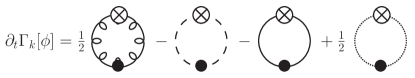
Figure 1: Partially hadronised version of the FRG flow for QCD. The loops denote the gluon, ghost, quark and meson contributions, respectively. The crosses mark the FRG regulator term.

Fig. 1 shows the pictorial representation of the FRG flow of QCD, where the first two loops represent the gluon and ghost contributions, respectively, whereas the third loop denotes the quark degrees of freedom. The fourth loop corresponds to mesonic degrees of freedom which have been introduced via the dynamical hadronisation technique Gies and Wetterich (2002, 2004); Pawlowski (2007); Floerchinger and Wetterich (2009).

It is well-established that the ghost-gluon sector decouples from the matter dynamics below the chiral and deconfinement temperatures, see e.g. Fischer et al. (2009). In terms of the flow equation, Fig. 1, this means that in this regime we are only left with the dynamical matter sector given by the last two loops, explicitly

$$\partial_{t}\Delta\Gamma_{k}[\bar{A};\phi] = -\operatorname{Tr}\left(G_{q}[\bar{A};\phi]\partial_{t}R_{q}\right)$$ (1)

$$+\ \frac{1}{2}\operatorname{Tr}\left(G_{H}[\bar{A};\phi]\partial_{t}R_{H}\right)\,.$$

The full field content is collected in $\phi~{}=~{}(a,\ c,\ \bar{c},\ q,\ \bar{q},\ H)$ . In the non-perturbative domain of QCD the spectrum is gapped and only light constituent quarks ($q,\bar{q}$) and the corresponding hadrons ($H$) do not decouple, whereas the ghost ($c,\bar{c}$) and gluon ($A=\bar{A}+a$) fields, as well as the heavy matter sector act as spectators at low densities. Here we have decomposed the gauge fields into a constant background $\bar{A}$ and a fluctuating part $a$.

The effective action of full QCD can then be written as

$$\Gamma_{k}=\beta\mathcal{V}V[A_{0}]+\Delta\Gamma_{k}[\bar{A}_{0},\phi]\,,$$ (2)

where $\mathcal{V}$ is the spatial volume and $\beta=1/T$ the inverse temperature. In Eq. (2), the first term denotes the QCD glue potential, encoding the ghost-gluon dynamics in the presence of matter fields. The second term contains the matter contribution coupled to a background gluon field $\bar{A}_{0}$. This contribution is well-described in terms of low-energy chiral models, such as the Nambu–Jona-Lasinio (NJL) and quark-meson (QM) models, coupled to Polyakov loops. In this work we make use of a Polyakov–quark-meson (PQM) truncation Schaefer et al. (2007); Skokov et al. (2010a); Herbst et al. (2011) for the matter sector at low energies. It is important to notice that the glue potential $V[A_{0}]$ in full QCD is different from its Yang-Mills counterpart due to unquenching effects, see e.g. the discussion in Herbst et al. (2013); Haas et al. (2013). The glue potential used in effective models, on the other hand, is usually fitted to pure Yang-Mills lattice results Pisarski (2000); Scavenius et al. (2002); Ratti et al. (2006); Roessner et al. (2007); Fukushima (2008); Lo et al. (2013).

To approximate unquenching effects we formulate the glue potential in terms of the reduced temperature

$$t=\frac{T-T_{\rm cr}}{T_{\rm cr}}\,,$$ (3)

and write $V_{\rm YM/glue}[A_{0};t]\,.$ To be more precise, there are also two reduced temperatures, defined in terms of the critical temperatures $T_{\rm cr}=T_{\rm cr}^{\rm YM}$ and $T_{\rm cr}=T_{\rm cr}^{\rm glue}$. One important effect of dynamical matter fields is to lower the scale $T_{\rm cr}^{\rm glue}$ as compared to $T_{\rm cr}^{\rm YM}$, which can be used to model the unquenching effects Schaefer et al. (2007); Herbst et al. (2011). In the present work we remedy the scale mismatch with the help of first-principles QCD results, see Haas et al. (2013) for a detailed discussion. There, the FRG results for the glue potential in YM theory Braun et al. (2010a, b); Fister and Pawlowski (2013) and QCD with two massless quark flavours Braun et al. (2011) have been compared, see also Fischer et al. (2013) for results with $2+1$ flavours. It was found that, apart from a rescaling, the shape of the glue potential in both theories is very similar close to $T_{\rm cr}$, see Figs. 5 and 7 in Haas et al. (2013). The simple linear relation

$$t_{\rm YM}(t_{\rm glue})\approx 0.57\,t_{\rm glue}\,,$$ (4)

is already capable of connecting the scales of both theories. In this manner, a potential $V_{\rm glue}[\Phi,\bar{\Phi};t]=V_{\rm YM}[\Phi(A_{0}),\bar{\Phi}(A_{0});t_{\rm YM}(t)]$ is defined, where $\Phi,\ \bar{\Phi}$ denote the Polyakov loop and its conjugate. Note that the relation Eq. (4) holds only for small and moderate temperatures, as the slope saturates at high scales, where the perturbative limit is reached.

In the following, Eq. (4) is used to account for the scale mismatch introduced by the fit of the PQM glue potential to YM lattice data. The only quantity left to fix is then the critical temperature of the glue sector, $T_{\rm cr}^{\rm glue}$. This value can in principle also be deduced from the QCD glue potential, see Braun et al. (2011), and yields $T_{\rm cr}^{\rm glue}(N_{f}=2)=203$ MeV. Since the absolute scale in Braun et al. (2011) was not computed in a chiral extrapolation of the theory with physical quark masses, we consider $T_{\rm cr}^{\rm glue}$ as an open parameter in the range

$$180~{}\text{MeV}\lesssim T_{\rm cr}^{\rm glue}\lesssim T_{\rm cr}^{\rm YM}=270~{}\text{MeV}\,,$$ (5)

constrained by the estimates in Schaefer et al. (2007); Herbst et al. (2011).

III Polyakov–Quark-Meson Model

In the following we provide some details of the Polyakov–quark-meson (PQM) model Schaefer et al. (2007); Skokov et al. (2010a); Herbst et al. (2011) and discuss the corresponding FRG flow equation at leading order in an expansion in derivatives.

The chiral sector of this model is given by the well-known quark-meson model Ellwanger and Wetterich (1994); Jungnickel and Wetterich (1996a); Schaefer and Pirner (1997); Berges et al. (1999); Schaefer and Wambach (2005). The integration of the gluonic degrees of freedom results in a potential for the Polyakov-loops ($\Phi(A_{0}),\,\bar{\Phi}(A_{0})$). They are coupled to the matter sector via the quark fields.

III.1 Setup

The Euclidean Lagrangian for the PQM model reads

$$\mathcal{L}_{\rm PQM} = \bar{q}\left({D\!\hbox to0.0pt{\hss/}}\,+h\,T^{a}(\sigma_{a}+i\gamma_{5}\pi_{a})+\mu\gamma_{0}\right)q$$ (6)

$$+\ \mathcal{L}_{m}+\ V_{\rm glue}(\Phi,\bar{\Phi};t)\,,$$

with a flavour-blind Yukawa coupling $h$ and the covariant derivative ${D\!\hbox to0.0pt{\hss/}}\,(\Phi)=\gamma_{\mu}\partial_{\mu}-i\,g\gamma_{0}A_{0}(\Phi)$ coupling the quark fields to the Polyakov loop. In this work we assume isospin symmetry in the light sector and use a flavour-blind chemical potential $\mu\,.$ The mesonic Lagrangian is given by Lenaghan et al. (2000); Schaefer and Wagner (2009); Mitter and Schaefer (2013)

$$\mathcal{L}_{m} = \operatorname{Tr}(\partial_{\mu}\Sigma\partial_{\mu}\Sigma^{\dagger})+U(\rho_{1},\tilde{\rho}_{2})+c\,\xi$$ (7)

$$-\ \operatorname{Tr}\left[C(\Sigma+\Sigma^{\dagger})\right]\,.$$

Here, the field $\Sigma$ is a complex $(3\times 3)$-matrix

$$\Sigma=\Sigma_{a}T^{a}=(\sigma_{a}+i\pi_{a})T^{a}\,,$$ (8)

where $\sigma_{a}$ denotes the scalar and $\pi_{a}$ the pseudo-scalar meson nonets and the Hermitian generators of the flavour $U(3)$ symmetry are defined via the Gell-Mann matrices as $T^{a}=\lambda^{a}/2\,.$ It is advantageous to rotate into the non-strange–strange basis via

$$\begin{pmatrix}\sigma_{x}\\ \sigma_{y}\end{pmatrix}=\frac{1}{\sqrt{3}}\begin{pmatrix}\sqrt{2}&1\\ 1&-\sqrt{2}\end{pmatrix}\begin{pmatrix}\sigma_{0}\\ \sigma_{8}\end{pmatrix}\,,$$ (9)

with $\sigma_{x}$ the non-strange and $\sigma_{y}$ the strange condensate. Then, the explicit symmetry breaking term consistent with isospin symmetry takes the simple form $\operatorname{Tr}\left[C(\Sigma+\Sigma^{\dagger})\right]\to c_{x}\sigma_{x}+c_{y}\sigma_{y}$ , with $c_{x},c_{y}$ governing the bare light and strange quark masses, respectively.

The meson potential $U$ can be expressed via the chiral invariants $\rho_{i}=\operatorname{Tr}\left[(\Sigma\Sigma^{\dagger})^{i}\right]$, $i=1,\,\dots,\,N_{f}$ Jungnickel and Wetterich (1996b). In the ($2+1$)-flavour approximation, where $\sigma_{3}=0$, $\rho_{3}$ can be expressed in terms of the other invariants and we use the set $\{\rho_{1},\,\tilde{\rho}_{2},\,\xi\}$ with

$$\rho_{1} = \frac{1}{2}\left(\sigma_{x}^{2}+\sigma_{y}^{2}\right)\,,$$

$$\tilde{\rho}_{2} = \rho_{2}-\frac{1}{3}\rho_{1}^{2}=\frac{1}{24}\left(\sigma_{x}^{2}-2\sigma_{y}^{2}\right)^{2}\,,$$

$$\xi = \det(\Sigma)+\det(\Sigma^{\dagger})=\frac{\sigma_{x}^{2}\sigma_{y}}{2\sqrt{2}}\,.$$ (10)

Here, $\xi$ represents the ’t Hooft determinant ’t Hooft (1976a, b), rewritten in the mesonic language Kobayashi et al. (1971); ’t Hooft (1986), and as such implements the chiral $U_{A}(1)$ anomaly. The strength of its coupling, $c$, determines the mass splitting between the $\eta$, $\eta^{\prime}$ and pions, see e.g. Mitter and Schaefer (2013); Schaefer and Wagner (2009); Schaefer and Mitter (2013) for a detailed discussion.

Furthermore, the quasi-particle energies of the quarks and mesons are given by $E_{i}=\sqrt{k^{2}+m_{i}^{2}}$, $i~{}\in~{}\{l,\,s,\,j\}$ with $j\in\{\sigma,\,a_{0},\,\kappa,\,f_{0},\,\pi,\,K,\,\eta,\,\eta^{\prime}\}$. The masses themselves are defined as

$$m_{l} = h\frac{\langle\sigma_{x}\rangle}{2}\,,$$

$$m_{s} = h\frac{\langle\sigma_{y}\rangle}{\sqrt{2}}\,,$$ (11)

for the light and strange quarks, respectively, and

$$\{m_{j}^{2}\}=\text{eig}\left\{H_{\Sigma}\left(U(\rho_{1},\tilde{\rho}_{2})+c\xi\right)\right\}$$ (12)

for the mesons. Here, $H_{\Sigma}(.)$ denotes the Hessian w.r.t. $\Sigma$ and $\text{eig}\{.\}$ denotes the set of eigenvalues of the given operator. For further details on this model we refer the reader to Lenaghan et al. (2000); Schaefer and Wagner (2009); Mitter and Schaefer (2013). The two-flavour case considered in Sec. IV.2 is obtained by omitting the strange quark sector as well as all mesons except the sigma and pions.

What is now left is to specify the glue potential $V_{\rm glue}$. We have argued above that we can use the YM-based parametrisations $\mathcal{U}$ of the glue potential and modify the scale according to QCD FRG results, Eq. (4). Several parametrisations of the Polyakov-loop potential have been put forward in the recent years Pisarski (2000); Scavenius et al. (2002); Ratti et al. (2006); Roessner et al. (2007); Fukushima (2008); Fukushima and Kashiwa (2013); Lo et al. (2013). In the main text we only show results for a polynomial version, introduced in Pisarski (2000); Ratti et al. (2006)

$$\frac{\mathcal{U}_{\rm poly}(\Phi,\bar{\Phi};t)}{T^{4}} = -\frac{b_{2}(t)}{2}\Phi\bar{\Phi}-\ \frac{b_{3}}{6}\left(\Phi^{3}+\bar{\Phi}^{3}\right)$$ (13)

$$+\ \frac{b_{4}}{4}\left(\Phi\bar{\Phi}\right)^{2}\,.$$

The temperature-dependent coefficient, expressed in terms of the reduced temperature, is given by

$$b_{2}(t)=a_{0}+\frac{a_{1}}{1+t}+\frac{a_{2}}{(1+t)^{2}}+\frac{a_{3}}{(1+t)^{3}}\,.$$ (14)

The parameters $a_{i},\,b_{i}$ of Eqs. (13) and (14) have been determined in Ratti et al. (2006) by a fit to pure Yang-Mills lattice results to be

$$a_{0}=6.75\,,\ a_{1}=-1.95\,,\ a_{2}=2.625\,,\ a_{3}=-7.44$$ (15)

and

$$b_{3}=0.75\,,\quad b_{4}=7.5\,.$$ (16)

We use the lattice result for the pressure to fix the open parameter $T_{\rm cr}^{\rm glue}=210$ MeV in $\mathcal{U}(\Phi,\bar{\Phi};t)$. A discussion of the dependence of our results on this choice and on the parametrisation of $\mathcal{U}$ can be found in the appendix.

III.2 Fluctuations in the PQM model

In the present work we go beyond the mean-field approximation used in Haas et al. (2013) and apply the FRG to include quantum and thermal fluctuations of the PQM model. This provides us with a more realistic description of the chiral and deconfinement phase transitions. In fact it has been shown previously, see e.g. Schaefer and Wambach (2005), that fluctuations smear out the phase transition, yielding smoother transitions that are in better agreement with lattice results.

The flow equation for the two-flavour PQM model has been derived previously in Skokov et al. (2010a); Herbst et al. (2011) while the flow of the $(2+1)$-flavour quark-meson model is discussed in depth in Mitter and Schaefer (2013). It is then straight-forward to deduce the flow equation of the full $(2+1)$-flavour PQM model

$$\partial_{t}\Omega_{k}=\frac{k^{5}}{12\pi^{2}}\left\{\sum_{i=1}^{2N_{f}^{2}}\frac{1}{E_{i}}\coth\left(\frac{E_{i}}{2T}\right)\right.$$ (17)

$$\quad\left.-\frac{8N_{c}}{E_{l}}\left[1-N_{l}(T,\mu;\Phi,\bar{\Phi})-N_{\bar{l}}(T,\mu;\Phi,\bar{\Phi})\right]\right.$$

$$\quad\left.-\frac{4N_{c}}{E_{s}}\left[1-N_{s}(T,\mu;\Phi,\bar{\Phi})-N_{\bar{s}}(T,\mu;\Phi,\bar{\Phi})\right]\right\}\,.$$

The Polyakov-loop extended quark/anti-quark occupation numbers are given by

$$N_{q}(T,\mu;\Phi,\bar{\Phi})=\hskip 148.0pt$$ (18)

$$\dfrac{1+2\bar{\Phi}e^{(E_{q}-\mu)/T}+\Phi e^{2(E_{q}-\mu)/T}}{1+3\bar{\Phi}e^{(E_{q}-\mu)/T}+3\Phi e^{2(E_{q}-\mu)/T}+e^{3(E_{q}-\mu)/T}}\,,$$

and $N_{\bar{q}}(T,\mu;\Phi,\bar{\Phi})\equiv N_{q}(T,-\mu;\bar{\Phi},\Phi)$ for $q=l,s$.

Note that we restrict ourselves to leading order in a derivative expansion and neglect the running of any couplings involving quark interactions. The RG running of the mesonic couplings, on the other hand, is encoded in the scale-dependent effective potential $\Omega_{k}$.

In order to solve the flow Eq. (17), we have to specify an initial potential at the cutoff scale $\Lambda$. In this work we have chosen $\Lambda=1$ GeV, in accordance with our interpretation of the quark-meson model as a low-energy effective description. We keep only renormalisable terms in the mesonic potential at the cutoff scale and restrict ourselves to only two chiral invariants $\rho_{1},\tilde{\rho}_{2}$, cf. the discussion in Mitter and Schaefer (2013)

$$U_{\Lambda}(\rho_{1},\tilde{\rho}_{2})=a_{10}\rho_{1}+a_{01}\tilde{\rho}_{2}+\frac{a_{20}}{2}\rho_{1}^{2}\,.$$ (19)

The parameters are fixed to $a_{10}=(972.63~{}\text{ MeV})^{2},\,a_{01}=50,\,a_{20}=2.5$ which, together with the choices $h~{}=~{}6.5$ for the Yukawa coupling, $c=-4807.84$ MeV for the ’t Hooft–determinant coupling and explicit breaking strengths $c_{x}=(120.73~{}\text{MeV})^{3}$ and $c_{y}=(336.41~{}\text{MeV})^{3}$, reproduces the physical spectrum as well as the pion and kaon decay constants in the vacuum Beringer et al. (2012). In particular, we have chosen a sigma-meson mass of $m_{\sigma}=400$ MeV. In Appendix .3 we discuss the dependence of our results on this choice.

At temperatures $2\pi T\gtrsim\Lambda\,,$ thermal fluctuations become important also at scales above the cutoff $k>\Lambda$. These thermal fluctuations are, however, not taken into account in the solution to the flow Eq. (17) with finite cutoff $\Lambda$. Therefore, the initial potential $\Omega_{\Lambda}$ is not fully independent of temperature, which is quantitatively important in the region $2\pi T\gtrsim\Lambda$. On the other hand, this temperature dependence of the initial potential $\Omega_{\Lambda}$ is also governed by the flow Eq. (17) and can be obtained by integrating the vacuum flow from the cutoff $\Lambda$ up to a scale $\bar{\Lambda}\gg 2\pi T$ and subsequently integrating the finite temperature flow down to $\Lambda$ again

$$\Delta\Omega_{\Lambda}(T,\mu)=\int_{\Lambda}^{\bar{\Lambda}}\frac{dk}{k}\left(\partial_{t}\Omega_{k}(T,\mu)-\partial_{t}\Omega_{k}(0,0)\right)\,.$$ (20)

This procedure is equivalent to a change of the initial scale from $\Lambda$ to $\bar{\Lambda}$, while keeping the infrared physics fixed, i.e. a change in the renormalisation scale. However, as we expect mesonic fluctuations to be less important at scales $k>\Lambda=1$ GeV, we approximate the difference by the purely fermionic contribution to Eq. (17). Since the fermionic contribution to the flow is independent of $\Omega_{k}$, the approximate temperature dependence of $\Omega_{\Lambda}$ is given by the simple integral Braun et al. (2004); Herbst et al. (2011)

$$\Delta\Omega_{\Lambda} = \left.\int^{\infty}_{\Lambda}dk\frac{k^{4}}{12\pi^{2}}\right\{$$

$$\quad\quad\frac{8N_{c}}{E_{l}}\left[N_{l}(T,\mu;\Phi,\bar{\Phi})+N_{\bar{l}}(T,\mu;\Phi,\bar{\Phi})\right]$$

$$\quad\left.+\ \frac{4N_{c}}{E_{s}}\left[N_{s}(T,\mu;\Phi,\bar{\Phi})+N_{\bar{s}}(T,\mu;\Phi,\bar{\Phi})\right]\right\}\,.$$

Here, we have chosen $\bar{\Lambda}=\infty$, since the fermionic difference flow is finite. Finally we obtain

$$\Omega_{\Lambda}(T,\mu;\sigma_{x},\sigma_{y},\Phi,\bar{\Phi}) = U_{\Lambda}(\rho_{1},\tilde{\rho}_{2})+\,\mathcal{U}(\Phi,\bar{\Phi};t)$$ (22)

$$+\ \Delta\Omega_{\Lambda}(T,\mu;\sigma_{x},\sigma_{y},\Phi,\bar{\Phi})\,,$$

for the initial potential at the cutoff scale $\Lambda$, including fermionic temperature corrections.

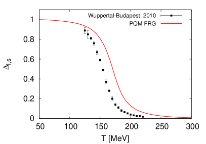
Figure 2: Temperature dependence of the subtracted chiral condensate: the FRG curve is compared to the lattice result by the Wuppertal-Budapest collaboration Borsanyi et al. (2010a).

IV Results

IV.1 QCD Crossover

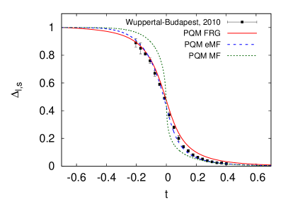
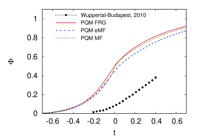
Figure 3: Temperature dependence of the subtracted chiral condensate (left) and Polyakov loop (right). The FRG result is compared to the lattice result of the Wuppertal-Budapest collaboration, Borsanyi et al. (2010a), as well as to the mean-field result. See text for comments on the Polyakov loop in continuum approaches.

From the solution to the flow Eq. (17) we can determine the phase structure and thermodynamics of the PQM model. For the time being, we restrict ourselves to vanishing chemical potential. This has the advantage that in this limit the Polyakov loop and its conjugate coincide, $\bar{\Phi}=\Phi$. Hence, the numerical effort to solve the equations of motion (EoM)

$$\left.\dfrac{\partial\Omega_{k\to 0}}{\partial\sigma_{x}}\right|_{\chi_{0}}=\left.\dfrac{\partial\Omega_{k\to 0}}{\partial\sigma_{y}}\right|_{\chi_{0}}=\left.\dfrac{\partial\Omega_{k\to 0}}{\partial\Phi}\right|_{\chi_{0}}=0\,,$$ (23)

which determine the order parameters $\chi_{0}=\left(\sigma_{x},\sigma_{y},\Phi\right)$ for given temperature and chemical potential, is drastically reduced. A discussion of the numerical method used to solve this multi-dimensional system of partial differential equations can be found in Strodthoff et al. (2012); Mitter and Schaefer (2013).

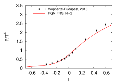
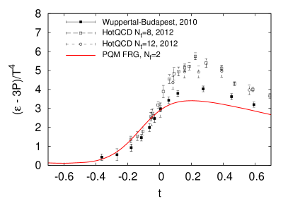
Figure 4: FRG result for the pressure (left) and interaction measure (right) for two quark flavours, compared to the $(2+1)$-flavour lattice results Bazavov (2013); Borsanyi et al. (2010b). See text for details.

In Fig. 2 our result for the subtracted chiral condensate,

$$\Delta_{l,s}=\frac{\left(\sigma_{x}-\frac{c_{x}}{c_{y}}\sigma_{y}\right)_{T}}{\left(\sigma_{x}-\frac{c_{x}}{c_{y}}\sigma_{y}\right)_{T=0}}$$ (24)

is shown in comparison with the lattice result by the Wuppertal-Budapest collaboration Borsanyi et al. (2010a). Due to the finite quark masses, we find a smooth crossover and there is no exact definition of the transition temperature. Nevertheless, it is customary to associate a transition temperature with the peak position of the temperature derivative of the order parameter, $d\Delta_{l,s}/dT$. Using this definition, we obtain $T_{\chi}=172$ MeV for the chiral crossover temperature, and similarly $T_{d}=163$ MeV for the Polyakov-loop related transition via $d\Phi/dT$. Both values agree roughly with the transition region on the lattice $(147-165)$ MeV Borsanyi et al. (2010a) and the pseudocritical temperatures $T_{\chi}=157\pm{3}$ MeV Borsanyi et al. (2010a) and $T_{\chi}=154\pm{9}$ MeV Bazavov et al. (2012).

Note that, apart from a shift along the temperature axis,the slope of our FRG result for the subtracted condensate coincides with the lattice one, cf. Figs. 2 and 3. This indicates that the relative strength of the relevant dynamics is included properly. However, there is a difference in the absolute scale, $T_{\chi}$, in our calculation and the lattice. This is to some extent related to our choice of the sigma meson mass. From experiment it is known that the $\sigma$ ($f_{0}(500)$) is a broad resonance, $(400-550)-i(200-350)$ MeV Beringer (Particle Data Group). It has been shown previously, see e.g. Schaefer and Wagner (2009), that a lower sigma mass results in a lower chiral transition temperature, while the slope of the condensate is only changed marginally. For the curve shown in Fig. 2 the value $m_{\sigma}=400~{}$MeV has been used. We have checked that for lower values, entailing stronger mesonic fluctuations, the result is shifted even closer to the lattice one. However, the value of $m_{\sigma}=400$ MeV is already at the lower experimental boundary, hence we refrain from using a lower mass in the following. The impact of this mass parameter on thermodynamics is also discussed in Appendix .3.

The axial anomaly similarly influences the transition. It has been demonstrated in Mitter and Schaefer (2013) that the transition temperature is reduced for vanishing anomaly coupling, $c=0$. In fact, with our choice of $m_{\sigma}=400~{}$MeV and $c=0$, the resulting condensate lies almost exactly on top of the lattice points. Note that in this case the $\eta^{\prime}$ meson would be an additional pseudo-Goldstone boson, again leading to enhanced fluctuations. However, this choice is unphysical and results in, e.g., a too high pressure at low temperatures. The use of a temperature-dependent anomaly coupling, $c(T)$, is expected to resolve this issue. In summary, we have found that for a correct description of the absolute scale, further mesonic fluctuations need to be included. Within our FRG treatment this would correspond to higher mesonic operators in our cutoff potential, $\Omega_{\Lambda}$. In full QCD such contributions are dynamically generated at higher scales, but we have omitted them in the present work since we restrict our cutoff action to contain renormalisable operators only.

We conclude that while the absolute scale, $T_{\chi}$, differs from the lattice one by about $10\%$ in our FRG calculation, the relative strength of the relevant dynamics of the transition is captured well. This is due to the inclusion of unquenching effects as well as matter fluctuations. We postpone the improvement of our scale-setting procedure to future work and concentrate on the discussion of the dynamics of the transition in the following. To this end, all results are expressed in terms of the reduced temperature $t=(T-T_{\chi})/T_{\chi}$. This choice allows us to compare the overall shape - and thereby the proper inclusion of the relevant dynamics - of the observables, while a mismatch of the critical temperatures is scaled out.

Fig. 3 shows the subtracted chiral condensate (left) as well as the Polyakov loop (right) in terms of the reduced temperature. As argued above, we observe excellent agreement between the FRG (solid line) and lattice (symbols) result for the chiral condensate, especially at temperatures below $T_{\chi}$. In turn, for temperatures above the transition the present model overestimates the importance of mesonic fluctuations, and the FRG result for the order parameter is above the lattice result. The use of dynamical hadronisation, Gies and Wetterich (2002, 2004); Pawlowski (2007); Floerchinger and Wetterich (2009), should compensate this effect.

For comparison, in Fig. 3 we also show results from a PQM mean-field calculation without (“MF”, dotted line) and with (“eMF“, dashed line) the fermionic vacuum loop contribution Skokov et al. (2010b); Andersen et al. (2011); Gupta and Tiwari (2012); Schaefer and Wagner (2012). Note that we fix the remaining parameters of the model, $m_{\sigma}$ and $T_{\rm cr}^{\rm glue}$, by comparing the pressure to the lattice pressure, cf. discussion in Appendix .2. In this manner, the effect of fluctuations is partially included in the model parameters. This results in different parameter values for the mean-field and FRG calculations. We use $m_{\sigma}=500$ MeV and $T_{\rm cr}^{\rm glue}=210$ MeV for the standard mean-field calculation, as discussed in Haas et al. (2013); Stiele et al. (2012) and $m_{\sigma}=400$ MeV, $T_{\rm cr}^{\rm glue}=260$ MeV for the extended mean-field calculation. However, it is clear from, e.g., Fig. 3, that a modification of the parameters is not sufficient to describe the full dynamics of the transition. The inclusion of fluctuations, as done in our FRG setup, is crucial to reproduce the slope of the order parameter as well as thermodynamic observables correctly.

In fact, the pseudocritical temperature of the standard mean-field approximation is closer to the lattice one than our FRG result, $T_{\chi}=T_{d}=158$ MeV. However, this approach neglects mesonic fluctuations, and the transition comes out too steep, see Fig. 3. Including the fermionic vacuum fluctuations yields too high pseudocritical temperatures, $T_{\chi}=181$ MeV and $T_{d}=173$ MeV. Compared to the standard MF result, on the other hand, the slope of the condensate is reduced.

A word of caution needs to be added concerning the Polyakov loop, Fig. 3 (right). It is well-known that the definitions of this quantity used on the lattice, $\langle\Phi\rangle$, and the present continuum formulation, $\Phi[\langle A_{0}\rangle]$, differ and a direct comparison is not possible. In view of this, we do not expect agreement of these two observables. However, it can be shown that the continuum definition serves as an upper bound for the lattice one, $\Phi[\langle A_{0}\rangle]\geq~{}\langle\Phi\rangle\,,$ up to renormalisation issues, cf. Braun et al. (2010a); Marhauser and Pawlowski (2008). Hence, an approximate coincidence of the respective crossover regions is still anticipated. Indeed, we find that our transition temperature, defined by the inflection point of the Polyakov loop, roughly agrees with the transition region found on the lattice.

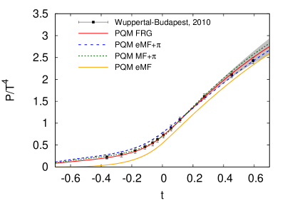
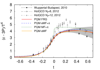
Figure 5: $(2+1)$-flavour FRG results for the pressure (left) and interaction measure (right) compared to the lattice, Bazavov (2013); Borsanyi et al. (2010b), and mean-field results. See text for details.

IV.2 Thermodynamics: $N_{f}=2$

Within the FRG framework, the full quantum effective potential is defined by the effective average potential $\Omega_{k}$ in the infrared, evaluated on the solution of the EoM,

$$\Omega(T,\mu)=\Omega_{k\to 0}(T,\mu)|_{\chi_{0}}\,.$$ (25)

The pressure of the system is then given by the negative of the effective potential, normalised in the vacuum

$$P=-\Omega(T,\mu)+\Omega(0,0)\,,$$ (26)

and serves as a thermodynamic potential, from which we can deduce other bulk thermodynamic quantities in the standard way. In particular, we are interested in the free energy density

$$\epsilon=-P+Ts+\sum_{f}\mu_{f}n_{f}\,,$$ (27)

with the entropy density $s=\partial P/\partial T$ and the quark number densities $n_{f}=\partial P/\partial\mu_{f}$ for $f=u,d,s$ . Moreover, we consider the interaction measure

$$\Delta=\epsilon-3P\,,$$ (28)

which quantifies the deviation from the equation of state of an ideal gas, $\epsilon=3P$.

We compare these quantities to results of the HotQCD collaboration, Bazavov (2013), using the HISQ action and temporal lattice extents of $N_{\tau}=8,12$ as well as to the continuum extrapolated results of the Wuppertal-Budapest collaboration Borsanyi et al. (2010b).

We start our discussion of thermodynamic quantities by studying the two-flavour case. The flow equation of the two-flavour PQM model has previously been discussed in Skokov et al. (2010a); Herbst et al. (2011). Here, we use the parameter set given in Herbst et al. (2013), with $m_{\sigma}=540$ MeV. To our knowledge, there are no recent two-flavour lattice results for thermodynamics available. This entails that we cannot fix the remaining parameter, $T_{\rm cr}^{\rm glue}$, to, e.g., the lattice pressure. Instead we have chosen the same value as for $2+1$ flavours, $T_{\rm cr}^{\rm glue}=210$ MeV, see also our discussion in Sec. IV.3 below. This value is close to the phenomenological HTL estimate, $T_{\rm cr}^{\rm glue}(N_{f}=2)=208$ MeV put forward in Schaefer et al. (2007); Herbst et al. (2011) and the FRG estimate, $T_{\rm cr}^{\rm glue}=203$ MeV of Braun et al. (2011). Furthermore, this choice results in almost degenerate chiral and Polyakov-loop critical temperatures. Having fixed all parameters, the results of the present section serve as a prediction for the thermodynamics of two-flavour QCD.

In Fig. 4 we show the pressure (left) and interaction measure (right), both normalised by $T^{4}$. For comparison we also show the lattice results for $2+1$ flavours. Despite the fact that we only consider two quark flavours here, the overall agreement is rather good. At low temperatures, the lightest mesonic degrees of freedom, the pions, are expected to dominate the pressure. These are already included in the two-flavour model. At high temperatures, on the other hand, the two-flavour FRG result underestimates the $(2+1)$-flavour lattice value. This is expected due to the additional third quark species contributing to the lattice pressure at high $T$.

The right panel of Fig. 4 shows the interaction measure. Deviations from the lattice are more pronounced in this quantity due to the presence of derivatives in its definition. Of course we do not expect perfect agreement between our two-flavour computation and the $N_{f}=2+1$ lattice result. However, the strongest modifications are expected around the phase transition, where there are more light degrees of freedom contributing to the thermodynamics for $2+1$ flavours. In the low and high temperature regimes the quarks and mesons are heavy, respectively, and hence contribute less to the thermodynamic observables. This explains the surprisingly good agreement between the two and three flavour results. In fact, we find reasonable agreement with the lattice data below the phase transition, $t\leq 0$. While the peak height is underestimated, the increase in $\Delta/T^{4}$ around $T_{c}$ is similar to the lattice. Above $T_{c}$, the two-flavour curve lies below the lattice result.

IV.3 Thermodynamics: $N_{f}=2+1$

Next, we turn to the (2+1)-flavour model. Here, we can directly compare to the available (2+1)-flavour lattice results and fix our open parameter, $T_{\rm cr}^{\rm glue}\,$ by comparison of the pressure. Fig. 5 (left, solid line) then shows our result for the pressure, normalised by $T^{4}$, which agrees very well with the lattice result in the continuum limit. Near $t=0$ this is a consequence of our choice of $T_{\rm cr}^{\rm glue}$. The nice agreement with lattice data away from $T_{\chi}$, on the other hand, indicates that we have included all relevant degrees of freedom, especially below the transition temperature. The grey band gives an error estimate of our FRG result, which is obtained from the change of the threshold functions with respect to the temperature, at vanishing mass at the ultraviolet cutoff $\Lambda$. This results in

$$P\pm\Delta P(\Lambda,T) = P\left(1\pm\frac{2}{e^{\Lambda/T}-1}\right)\,.$$ (29)

The propagation of uncertainty in the interaction measure as a derived quantity has been taken into account via

$$\frac{d\left(P\pm\Delta P(\Lambda,T)\right)}{dT} = \frac{dP}{dT}\pm\frac{d\left(P\frac{2}{e^{\Lambda/T}-1}\right)}{dT}\,.$$ (30)

Also shown in Fig. 5 are the mean-field results. To achieve a better description of the thermodynamics at low $T$, we have augmented the MF and eMF results by the contribution of a thermal pion gas, where the pion in-medium mass is determined by the mean-field potential. Our two flavour FRG calculation, see Sec. IV.2, confirms that these are the relevant degrees of freedom below the phase transition. To highlight the impact of this pion contribution, we also show results for the pure eMF calculation in Fig. 5 (yellow, solid line). Strictly speaking, this contribution picks up a field-dependence via the in-medium pion mass, which would modify the equations of motion. Here, however, we consider it as a correction to the thermodynamic potential only, and hence neglect its backcoupling on the equations of motion. For consistency, we also neglect all terms containing field derivatives, $\partial{P_{\pi}}/\partial\phi_{i}$, in higher thermodynamic observables.

While the pressure of the mean-field approximation including pions (dotted line) lies above the FRG and lattice ones, the inclusion of the vacuum term (dashed line) results in an additional increase in $P$ at low $t$ and a decrease at high $t$. As expected, the omission of the pion contribution in the eMF calculation (solid, yellow line) yields a pressure that is too low, especially below the phase transition, where pions are expected to dominate the thermodynamics.

The interaction measure is displayed in the right panel of Fig. 5. Similarly to the other observables, also the interaction measure is too steep within the standard mean-field approximation. Including the vacuum term, the transition is smoothened out and already agrees quite well with the Wuppertal-Budapest results. Turning to our FRG result (red, solid curve), we find remarkably good agreement with the continuum extrapolated lattice result from the Wuppertal-Budapest collaboration. There is a stronger deviation from the HotQCD data, but we attribute this to the lacking continuum limit of their data. In fact it is observed that the peak height of $\Delta/T^{4}$ goes down as the continuum is approached, cf. Borsanyi et al. (2010b); Bazavov (2013). Although not shown explicitly, we want to stress that the drastic reduction of the peak height in the interaction measure towards the lattice results is due the inclusion of $t_{\rm YM}(t_{\rm glue})$ in both the FRG and mean-field approaches, see also Haas et al. (2013); Stiele et al. (2012).

In comparison to our two-flavour result, we see that the inclusion of the heavier strange quark and especially the full scalar and pseudoscalar meson nonets increases the peak height of the interaction measure and puts our curve right on top of the lattice result. At high temperatures we find that $\Delta/T^{4}$ decreases too slowly in our calculation. However, this is the region where our scale matching procedure, Eq. (4), ceases to be valid and corrections are expected.

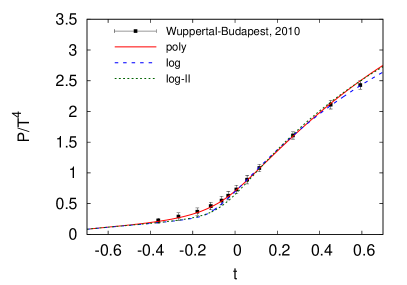
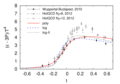
Figure 6: $(2+1)$-flavour FRG results for the pressure (left) and interaction measure (right) with polynomial (solid, red) Ratti et al. (2006), logarithmic (dashed, blue) Roessner et al. (2007) and enhanced logarithmic (dotted, green) Lo et al. (2013) Polyakov-loop potential with $T_{\rm cr}^{\rm glue}\,=210$ MeV.

V Conclusion and Outlook

We have investigated order parameters and thermodynamic observables of two and $2+1$ flavour QCD within effective Polyakov–quark-meson models. This type of models can be systematically related to full QCD, as e.g. discussed in Herbst et al. (2013); Haas et al. (2013). Thus far, the glue sector of these models is badly constrained. One often resorts to a Ginzburg–Landau-like ansatz for the glue potential obtained from fits to lattice Yang-Mills theory.

Recently, first-principles continuum results for the unquenched glue potentials have become available. These have been used to augment the glue sector considerably in a mean-field approach to the PQM model Haas et al. (2013). It was shown that by a simple rescaling of the temperature in the standard Yang-Mills based Polyakov-loop potentials one can already capture the essential glue dynamics of the unquenched system

In the present work, we have extended the previous investigation Haas et al. (2013) by additionally including thermal and quantum fluctuations via the functional renormalisation group. A comparison to lattice QCD simulations with $2+1$ flavours shows excellent agreement up to temperatures of approximately $1.3$ times the critical temperature. Therefore, we conclude that most of the relevant dynamics for the QCD crossover can already be captured within the PQM model. Additionally, we have put forward a prediction for the pressure and interaction measure for two quark flavours, where no recent lattice results with physical masses are available.

The present work serves as a benchmark of our system at vanishing chemical potential, which allows us to conclude that we have all relevant fluctuations included. Since our approach is not restricted to the zero chemical potential region we can now aim at the full phase diagram, $\mu\geq 0$ .

Acknowledgements

We thank L. Haas, L. Fister and J. Schaffner-Bielich for discussions and collaboration on related topics. This work is supported by the Helmholtz Alliance HA216/EMMI, by ERC-AdG-290623, by the FWF through grant P24780-N27 and Erwin-Schrödinger-Stipendium No. J3507, by the GP-HIR, by the BMBF grant OSPL2VHCTG and by CompStar, a research networking programme of the European Science Foundation.

Appendix: Parameter Dependence

In this appendix we estimate the parameter dependence of our results. In particular, we discuss the influence of the Polyakov-loop potential chosen, our choice of the glue critical temperature $T_{\rm cr}^{\rm glue}$ and the sigma-meson mass.

.1 Polyakov-loop Potential

	$T_{\chi}$ [MeV]	$T_{d}$ [MeV]
poly	172	163
log	170	146
log-II	172	156

Table 1: Chiral and deconfinement crossover temperatures for different parametrisations of the Polyakov-loop potential, all with $T_{\rm cr}^{\rm glue}=210\,\mathrm{MeV}$.

In the Polyakov-loop extended chiral models one is free to choose a parametrisation of the Polyakov-loop potential. It is customary to employ a Landau–Ginzburg-like ansatz and fit the parameters to available lattice data. However, in this manner only the region close to the minimum is constrained, not the overall shape. This is the reason why several different functional forms have been chosen in the past. In practise, when the Polyakov-loop is coupled to the matter sector, regions away from the minimum are probed and one should not expect to find exactly the same results with different versions of the potential.

In the main text we have presented results for a polynomial parametrisation Ratti et al. (2006). Here, we want to compare these results to those using a logarithmic version of the potential Roessner et al. (2007)

$$\frac{\mathcal{U}_{\rm log}(\Phi,\bar{\Phi};t)}{T^{4}}=-\frac{1}{2}a(t)\bar{\Phi}\Phi$$ (31)

$$\qquad\quad+\ b(t)\ln\left[1-6\bar{\Phi}\Phi+4\left(\Phi^{3}+\bar{\Phi}^{3}\right)-3\left(\bar{\Phi}\Phi\right)^{2}\right]\,,$$

In this variant, the logarithmic form arises from the integration of the Haar measure and constrains the Polyakov-loop variables $\Phi,\bar{\Phi}$ to values smaller than one.

Furthermore, we show results with the parametrisation recently proposed in Lo et al. (2013)

$$\frac{\mathcal{U}_{\rm log-II}(\Phi,\bar{\Phi};t)}{T^{4}}=\frac{\mathcal{U}_{\rm log}(\Phi,\bar{\Phi};t)}{T^{4}}$$

$$\qquad\qquad+\frac{c(t)}{2}\left(\Phi^{3}+\bar{\Phi}^{3}\right)+d(t)\left(\bar{\Phi}\Phi\right)^{2}\,.$$ (32)

The parameters of Eqs. (31) and (.1) have been fixed in Roessner et al. (2007) and Lo et al. (2013), respectively.

Tab. 1 summarises our FRG results for the transition temperatures using the initial values given in Sec. III.2 and these different Polyakov-loop potentials. Using the polynomial Polyakov-loop potential, the chiral and deconfinement transitions lie closer to each other than with the logarithmic ones.

In Fig. 6, the pressure (left) and interaction measure (right) are shown for $N_{f}=2+1$ and the three parametrisations. The pressure for the two logarithmic versions lies below the lattice result at low temperature, while the overall agreement is quite good also in this case. In the interaction measure, however, differences are seen more clearly. The trace anomaly resulting from the standard logarithmic potential rises much steeper than the one obtained with the polynomial version. The peak height, on the other hand, agrees well with the results of the Wuppertal-Budapest collaboration, independent of the parametrisation of the potential.

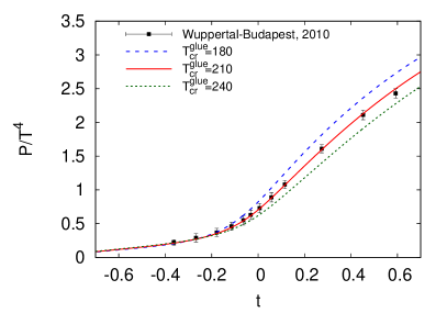
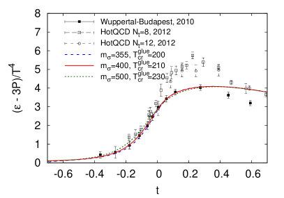
Figure 7: Pressure for different values of $T_{\rm cr}^{\rm glue}$ (left) and interaction measure for different choices of $m_{\sigma}$ with the corresponding optimal $T_{\rm cr}^{\rm glue}$ (right).

$m_{\sigma}$ [MeV]	$T_{\chi}$ [MeV]	$T_{\rm cr}^{\rm glue}$ [MeV]
$355$	$163$	$200$
$400$	$172$	$210$
$500$	$190$	$230$

Table 2: Chiral crossover temperatures for different values of the sigma-meson mass. In every calculation, the corresponding optimal value for $T_{\rm cr}^{\rm glue}$ as obtained from fixing the pressure has been used.

.2 Glue Critical Temperature

Next, we discuss the impact of the glue critical temperature, $T_{\rm cr}^{\rm glue}$. In the main text we have chosen $T_{\rm cr}^{\rm glue}=210$ MeV for $2+1$ flavours with physical anomaly strength. This value has been obtained by a comparison of the resulting pressure to the lattice results of the Wuppertal-Budapest collaboration. Fig. 7 (left) summarises the dependence of the pressure on $T_{\rm cr}^{\rm glue}$. In terms of the reduced temperature $t$, the effect of the glue critical temperature is to stretch the transition region, i.e. the transition becomes less steep for larger $T_{\rm cr}^{\rm glue}$.

.3 Sigma-Meson Mass

The sigma meson, $f_{0}(500)$ is a rather broad resonance, $(400-550)-i(200-350)$ MeV, which leaves us some freedom to fix this mass in our setup. The choice of this mass influences, e.g. the position of the phase transition and the location of a possible critical endpoint in the phase diagram Schaefer and Wagner (2009). For $2+1$ flavours we have fixed $m_{\sigma}=400$ MeV, see also our discussion in Sec. IV.1. In Tab. 2 we show the critical temperatures for different choices of the sigma-meson mass. Although the absolute value $T_{\chi}$ is quite susceptible to $m_{\sigma}$, we find that the thermodynamic observables in terms of the reduced temperature are not. This is demonstrated for the interaction measure in the right panel of Fig. 7. We have to stress, however, that this $m_{\sigma}$ independence is partially due to the fact that a change in the sigma-meson mass can be compensated to some degree by a change in $T_{\rm cr}^{\rm glue}$, see also Haas et al. (2013); Stiele et al. (2012).

References

- Braun et al. (2011) J. Braun, L. M. Haas, F. Marhauser, and J. M. Pawlowski, Phys.Rev.Lett. 106, 022002 (2011), arXiv:0908.0008 [hep-ph] .
- Herbst et al. (2013) T. K. Herbst, J. M. Pawlowski, and B.-J. Schaefer, Phys. Rev. D88, 014007 (2013), arXiv:1302.1426 [hep-ph] .
- Haas et al. (2013) L. M. Haas, R. Stiele, J. Braun, J. M. Pawlowski, and J. Schaffner-Bielich, Phys.Rev. D87, 076004 (2013), arXiv:1302.1993 [hep-ph] .
- Mitter and Schaefer (2013) M. Mitter and B.-J. Schaefer, (2013), arXiv:1308.3176 [hep-ph] .
- Litim and Pawlowski (1999) D. F. Litim and J. M. Pawlowski, World Sci. , 168 (1999), arXiv:hep-th/9901063 .
- Berges et al. (2002) J. Berges, N. Tetradis, and C. Wetterich, Phys.Rept. 363, 223 (2002), arXiv:hep-ph/0005122 .
- Pawlowski (2007) J. M. Pawlowski, Annals Phys. 322, 2831 (2007), arXiv:hep-th/0512261 .
- Gies (2012) H. Gies, Lect.Notes Phys. 852, 287 (2012), arXiv:hep-ph/0611146 .
- Schaefer and Wambach (2008) B.-J. Schaefer and J. Wambach, Phys.Part.Nucl. 39, 1025 (2008), arXiv:hep-ph/0611191 .
- Pawlowski (2011) J. M. Pawlowski, AIP Conf.Proc. 1343, 75 (2011), arXiv:1012.5075 [hep-ph] .
- Braun (2012) J. Braun, J.Phys. G39, 033001 (2012), arXiv:1108.4449 [hep-ph] .
- von Smekal (2012) L. von Smekal, Nucl.Phys.Proc.Suppl. 228, 179 (2012), arXiv:1205.4205 [hep-ph] .
- Braun et al. (2010a) J. Braun, H. Gies, and J. M. Pawlowski, Phys.Lett. B684, 262 (2010a), arXiv:0708.2413 [hep-th] .
- Fischer and Luecker (2013) C. S. Fischer and J. Luecker, Phys.Lett. B718, 1036 (2013), arXiv:1206.5191 [hep-ph] .
- Fister and Pawlowski (2013) L. Fister and J. M. Pawlowski, Phys.Rev. D88, 045010 (2013), arXiv:1301.4163 [hep-ph] .
- Fischer et al. (2013) C. S. Fischer, L. Fister, J. Luecker, and J. M. Pawlowski, (2013), arXiv:1306.6022 [hep-ph] .
- Meisinger and Ogilvie (1996) P. N. Meisinger and M. C. Ogilvie, Phys.Lett. B379, 163 (1996), arXiv:hep-lat/9512011 .
- Pisarski (2000) R. D. Pisarski, Phys.Rev. D62, 111501 (2000), arXiv:hep-ph/0006205 .
- Fukushima (2004) K. Fukushima, Phys.Lett. B591, 277 (2004), arXiv:hep-ph/0310121 .
- Megias et al. (2006) E. Megias, E. Ruiz Arriola, and L. Salcedo, Phys.Rev. D74, 065005 (2006), arXiv:hep-ph/0412308 .
- Ratti et al. (2006) C. Ratti, M. A. Thaler, and W. Weise, Phys.Rev. D73, 014019 (2006), arXiv:hep-ph/0506234 .
- Mukherjee et al. (2007) S. Mukherjee, M. G. Mustafa, and R. Ray, Phys.Rev. D75, 094015 (2007), arXiv:hep-ph/0609249 .
- Roessner et al. (2007) S. Roessner, C. Ratti, and W. Weise, Phys.Rev. D75, 034007 (2007), arXiv:hep-ph/0609281 .
- Sasaki et al. (2007) C. Sasaki, B. Friman, and K. Redlich, Phys. Rev. D75, 074013 (2007), arXiv:hep-ph/0611147 .
- Schaefer et al. (2007) B.-J. Schaefer, J. M. Pawlowski, and J. Wambach, Phys.Rev. D76, 074023 (2007), arXiv:0704.3234 [hep-ph] .
- Fraga and Mocsy (2007) E. Fraga and A. Mocsy, Braz.J.Phys. 37, 281 (2007), arXiv:hep-ph/0701102 .
- Fukushima (2008) K. Fukushima, Phys.Rev. D77, 114028 (2008), arXiv:0803.3318 [hep-ph] .
- Sakai et al. (2008) Y. Sakai, K. Kashiwa, H. Kouno, and M. Yahiro, Phys.Rev. D77, 051901 (2008), arXiv:0801.0034 [hep-ph] .
- Herbst et al. (2011) T. K. Herbst, J. M. Pawlowski, and B.-J. Schaefer, Phys.Lett. B696, 58 (2011), arXiv:1008.0081 [hep-ph] .
- Skokov et al. (2011) V. Skokov, B. Friman, and K. Redlich, Phys.Rev. C83, 054904 (2011), arXiv:1008.4570 [hep-ph] .
- Skokov et al. (2010a) V. Skokov, B. Stokic, B. Friman, and K. Redlich, Phys. Rev. C82, 015206 (2010a), arXiv:1004.2665 [hep-ph] .
- Schaefer and Wagner (2012) B.-J. Schaefer and M. Wagner, Phys.Rev. D85, 034027 (2012), arXiv:1111.6871 [hep-ph] .
- Braun and Janot (2011) J. Braun and A. Janot, Phys.Rev. D84, 114022 (2011), arXiv:1102.4841 [hep-ph] .
- Kamikado et al. (2013) K. Kamikado, N. Strodthoff, L. von Smekal, and J. Wambach, Phys.Lett. B718, 1044 (2013), arXiv:1207.0400 [hep-ph] .
- Braun and Herbst (2012) J. Braun and T. K. Herbst, (2012), arXiv:1205.0779 [hep-ph] .
- Fukushima and Kashiwa (2013) K. Fukushima and K. Kashiwa, Phys.Lett. B723, 360 (2013), arXiv:1206.0685 [hep-ph] .
- Mintz et al. (2013) B. W. Mintz, R. Stiele, R. O. Ramos, and J. Schaffner-Bielich, Phys.Rev. D87, 036004 (2013), arXiv:1212.1184 [hep-ph] .
- Stiele et al. (2013) R. Stiele, E. S. Fraga, and J. Schaffner-Bielich, (2013), arXiv:1307.2851 [hep-ph] .
- Strodthoff and von Smekal (2013) N. Strodthoff and L. von Smekal, (2013), arXiv:1306.2897 [hep-ph] .
- Stiele et al. (2012) R. Stiele, L. M. Haas, J. Braun, J. M. Pawlowski, and J. Schaffner-Bielich, PoS ConfinementX, 215 (2012), arXiv:1303.3742 [hep-ph] .
- Gies and Wetterich (2002) H. Gies and C. Wetterich, Phys.Rev. D65, 065001 (2002), arXiv:hep-th/0107221 .
- Gies and Wetterich (2004) H. Gies and C. Wetterich, Phys.Rev. D69, 025001 (2004), arXiv:hep-th/0209183 .
- Floerchinger and Wetterich (2009) S. Floerchinger and C. Wetterich, Phys.Lett. B680, 371 (2009), arXiv:0905.0915 [hep-th] .
- Fischer et al. (2009) C. S. Fischer, A. Maas, and J. M. Pawlowski, Annals Phys. 324, 2408 (2009), arXiv:0810.1987 [hep-ph] .
- Scavenius et al. (2002) O. Scavenius, A. Dumitru, and J. Lenaghan, Phys.Rev. C66, 034903 (2002), arXiv:hep-ph/0201079 .
- Lo et al. (2013) P. M. Lo, B. Friman, O. Kaczmarek, K. Redlich, and C. Sasaki, Phys. Rev. D 88, 074502 (2013), arXiv:1307.5958 [hep-lat] .
- Braun et al. (2010b) J. Braun, A. Eichhorn, H. Gies, and J. M. Pawlowski, Eur.Phys.J. C70, 689 (2010b), arXiv:1007.2619 [hep-ph] .
- Ellwanger and Wetterich (1994) U. Ellwanger and C. Wetterich, Nucl.Phys. B423, 137 (1994), arXiv:hep-ph/9402221 .
- Jungnickel and Wetterich (1996a) D. Jungnickel and C. Wetterich, Phys.Rev. D53, 5142 (1996a), arXiv:hep-ph/9505267 .
- Schaefer and Pirner (1997) B.-J. Schaefer and H.-J. Pirner, Nucl.Phys. A627, 481 (1997), arXiv:hep-ph/9706258 .
- Berges et al. (1999) J. Berges, D. Jungnickel, and C. Wetterich, Phys.Rev. D59, 034010 (1999), arXiv:hep-ph/9705474 .
- Schaefer and Wambach (2005) B.-J. Schaefer and J. Wambach, Nucl.Phys. A757, 479 (2005), arXiv:nucl-th/0403039 .
- Lenaghan et al. (2000) J. T. Lenaghan, D. H. Rischke, and J. Schaffner-Bielich, Phys.Rev. D62, 085008 (2000), arXiv:nucl-th/0004006 .
- Schaefer and Wagner (2009) B.-J. Schaefer and M. Wagner, Phys.Rev. D79, 014018 (2009), arXiv:0808.1491 [hep-ph] .
- Jungnickel and Wetterich (1996b) D. U. Jungnickel and C. Wetterich, Phys. Rev. D53, 5142 (1996b), arXiv:hep-ph/9505267 .
- ’t Hooft (1976a) G. ’t Hooft, Phys.Rev. D14, 3432 (1976a).
- ’t Hooft (1976b) G. ’t Hooft, Phys.Rev.Lett. 37, 8 (1976b).
- Kobayashi et al. (1971) M. Kobayashi, H. Kondo, and T. Maskawa, Prog.Theor.Phys. 45, 1955 (1971).
- ’t Hooft (1986) G. ’t Hooft, Phys.Rept. 142, 357 (1986).
- Schaefer and Mitter (2013) B.-J. Schaefer and M. Mitter, (2013), arXiv:1312.3850 [hep-ph] .
- Beringer et al. (2012) J. Beringer et al. (Particle Data Group), Phys.Rev. D86, 010001 (2012).
- Braun et al. (2004) J. Braun, K. Schwenzer, and H.-J. Pirner, Phys.Rev. D70, 085016 (2004), arXiv:hep-ph/0312277 .
- Borsanyi et al. (2010a) S. Borsanyi et al. (Wuppertal-Budapest Collaboration), JHEP 1009, 073 (2010a), arXiv:1005.3508 [hep-lat] .
- Strodthoff et al. (2012) N. Strodthoff, B.-J. Schaefer, and L. von Smekal, Phys.Rev. D85, 074007 (2012), arXiv:1112.5401 [hep-ph] .
- Bazavov (2013) A. Bazavov (HotQCD Collaboration), Nucl.Phys. A904-905, 877c (2013), arXiv:1210.6312 [hep-lat] .
- Borsanyi et al. (2010b) S. Borsanyi, G. Endrodi, Z. Fodor, A. Jakovac, S. D. Katz, et al., JHEP 1011, 077 (2010b), arXiv:1007.2580 [hep-lat] .
- Bazavov et al. (2012) A. Bazavov, T. Bhattacharya, M. Cheng, C. DeTar, H. Ding, et al., Phys.Rev. D85, 054503 (2012), arXiv:1111.1710 [hep-lat] .
- Beringer (Particle Data Group) J. Beringer (Particle Data Group) et al., Phys. Rev. D86, 010001 (2012).
- Skokov et al. (2010b) V. Skokov, B. Friman, E. Nakano, K. Redlich, and B.-J. Schaefer, Phys.Rev. D82, 034029 (2010b), arXiv:1005.3166 [hep-ph] .
- Andersen et al. (2011) J. O. Andersen, R. Khan, and L. T. Kyllingstad, (2011), arXiv:1102.2779 [hep-ph] .
- Gupta and Tiwari (2012) U. S. Gupta and V. K. Tiwari, Phys.Rev. D85, 014010 (2012), arXiv:1107.1312 [hep-ph] .
- Marhauser and Pawlowski (2008) F. Marhauser and J. M. Pawlowski, (2008), arXiv:0812.1144 [hep-ph] .