A Global Homogeneity Test for High-Dimensional Linear Regression

Camille Charbonnierlabel=u]camille.charbonnier@ensae.org [    Nicolas Verzelenlabel=v]nicolas.verzelen@supagro.inra.fr [    Fanny Villerslabel=w]fanny.villers@upmc.fr [
Abstract

This paper is motivated by the comparison of genetic networks based on microarray samples. The aim is to test whether the differences observed between two inferred Gaussian graphical models come from real differences or arise from estimation uncertainties. Adopting a neighborhood approach, we consider a two-sample linear regression model with random design and propose a procedure to test whether these two regressions are the same. Relying on multiple testing and variable selection strategies, we develop a testing procedure that applies to high-dimensional settings where the number of covariates p𝑝p is larger than the number of observations n1subscript𝑛1n_{1} and n2subscript𝑛2n_{2} of the two samples. Both type I and type II errors are explicitely controlled from a non-asymptotic perspective and the test is proved to be minimax adaptive to the sparsity. The performances of the test are evaluated on simulated data. Moreover, we illustrate how this procedure can be used to compare genetic networks on Hess et al breast cancer microarray dataset.

62H15,
62P10,
Gaussian graphical model,
two-sample hypothesis testing,
high-dimensional statistics,
multiple testing,
adaptive testing,
minimax hypothesis testing,
detection boundary,
keywords:
[class=AMS]
keywords:

, and

t1 t2 t3

1 Introduction

The recent flood of high-dimensional data has motivated the development of a vast range of sparse estimators for linear regressions, in particular a large variety of derivatives from the Lasso. Although theoretical guarantees have been provided in terms of prediction, estimation and selection performances (among a lot of others [7, 47, 34]), the research effort has only recently turned to the construction of high-dimensional confidence intervals or parametric hypothesis testing schemes [49, 8, 23, 29, 31]. Yet, quantifying the confidence surrounding coefficient estimates and selected covariates is essential in areas of application where these will nourrish further targeted investigations.

In this paper we consider the two-sample linear regression model with Gaussian random design.

Y(1)superscript𝑌1\displaystyle{Y}^{(1)} =\displaystyle= X(1)β(1)+ϵ(1)superscript𝑋1superscript𝛽1superscriptitalic-ϵ1\displaystyle{X}^{(1)}\beta^{(1)}+\epsilon^{(1)} (1)
Y(2)superscript𝑌2\displaystyle{Y}^{(2)} =\displaystyle= X(2)β(2)+ϵ(2).superscript𝑋2superscript𝛽2superscriptitalic-ϵ2\displaystyle{X}^{(2)}\beta^{(2)}+\epsilon^{(2)}\ . (2)

In this statistical model, the size p𝑝p row vectors X(1)superscript𝑋1X^{(1)} and X(2)superscript𝑋2X^{(2)} follow Gaussian distributions 𝒩(0p,Σ(1))𝒩subscript0𝑝superscriptΣ1{\mathcal{N}}(0_{p},\Sigma^{(1)}) and 𝒩(0p,Σ(2))𝒩subscript0𝑝superscriptΣ2{\mathcal{N}}(0_{p},\Sigma^{(2)}) whose covariance matrices remain unknown. The noise components ϵ(1)superscriptitalic-ϵ1\epsilon^{(1)} and ϵ(2)superscriptitalic-ϵ2\epsilon^{(2)} are independent from the design matrices and follow a centered Gaussian distribution with unknown standard deviations σ(1)superscript𝜎1\sigma^{(1)} and σ(2)superscript𝜎2\sigma^{(2)}. In this formal setting, our objective is to develop a test for the equality of β(1)superscript𝛽1\beta^{(1)} and β(2)superscript𝛽2\beta^{(2)} which remains valid in high-dimension.

Suppose that we observe an n1subscript𝑛1n_{1}-sample of (Y(1),X(1))superscript𝑌1superscript𝑋1(Y^{(1)},X^{(1)}) and an n2subscript𝑛2n_{2}-sample of (Y(2),X(2))superscript𝑌2superscript𝑋2(Y^{(2)},X^{(2)}) noted 𝐘(1)superscript𝐘1{\bf Y}^{(1)}, 𝐗(1)superscript𝐗1{\bf X}^{(1)}, and 𝐘(2)superscript𝐘2{\bf Y}^{(2)}, 𝐗(2)superscript𝐗2{\bf X}^{(2)}, with n1subscript𝑛1n_{1} and n2subscript𝑛2n_{2} remaining smaller than p𝑝p. Defining analogously ϵ(1)superscriptbold-italic-ϵ1\boldsymbol{\epsilon}^{(1)} and ϵ(2)superscriptbold-italic-ϵ2\boldsymbol{\epsilon}^{(2)}, we obtain the decompositions 𝐘(1)=𝐗(1)β(1)+ϵ(1)superscript𝐘1superscript𝐗1superscript𝛽1superscriptbold-italic-ϵ1{\bf Y}^{(1)}={\bf X}^{(1)}\beta^{(1)}+\boldsymbol{\epsilon}^{(1)} and 𝐘(2)=𝐗(2)β(2)+ϵ(2)superscript𝐘2superscript𝐗2superscript𝛽2superscriptbold-italic-ϵ2{\bf Y}^{(2)}={\bf X}^{(2)}\beta^{(2)}+\boldsymbol{\epsilon}^{(2)}. Given these observations, we want to test whether models (1) and (2) are the same, that is

{0:β(1)=β(2),σ(1)=σ(2),andΣ(1)=Σ(2)1:β(1)β(2) or σ(1)σ(2).cases:subscript0absentformulae-sequencesuperscript𝛽1superscript𝛽2formulae-sequencesuperscript𝜎1superscript𝜎2andsuperscriptΣ1superscriptΣ2:subscript1absentformulae-sequencesuperscript𝛽1superscript𝛽2 or superscript𝜎1superscript𝜎2\begin{cases}\mathcal{H}_{0}:&\beta^{(1)}=\beta^{(2)}\ ,\quad\sigma^{(1)}=\sigma^{(2)}\ ,\quad\text{and}\quad\Sigma^{(1)}=\Sigma^{(2)}\\ \mathcal{H}_{1}:&\beta^{(1)}\neq\beta^{(2)}\ \text{ or }\quad\sigma^{(1)}\neq\sigma^{(2)}\ .\\ \end{cases} (3)

In the null hypothesis, we include the assumption that the population covariances of the covariates are equal (Σ(1)=Σ(2)superscriptΣ1superscriptΣ2\Sigma^{(1)}=\Sigma^{(2)}), while under the alternative hypothesis the population covariances are not required to be the same. This choice of assumptions is primarely motivated by our final objective to derive homogeneity tests for Gaussian graphical models (see below). A discussion of the design hypotheses is deferred to Section 7.

1.1 Connection with two-sample Gaussian graphical model testing

This testing framework is mainly motivated by the validation of differences observed between Gaussian graphical models (modelling regulation networks) inferred from transcriptomic data from two samples [32, 17, 12] when looking for new potential drug or knock-out targets [24]. Following the development of univariate differential analysis techniques, there is now a surging demand for the detection of differential regulations between pairs of conditions (treated vs. placebo, diseased vs. healthy, exposed vs. control, …). Given two gene regulation networks inferred from two transcriptomic data samples, it is however difficult to disentangle differences in the estimated networks that are due to estimation errors from real differences in the true underlying networks.

We suggest to build upon our two-sample high-dimensional linear regression testing scheme to derive a global test for the equality of high-dimensional Gaussian graphical models inferred under pairs of conditions.

Formally speaking, the global two-sample GGM testing problem is defined as follows. Consider two Gaussian random vectors Z(1)𝒩(0,[Ω(1)]1)similar-tosuperscript𝑍1𝒩0superscriptdelimited-[]superscriptΩ11{Z}^{(1)}\sim\mathcal{N}(0,[\Omega^{(1)}]^{-1}) and Z(2)𝒩(0,[Ω(2)]1)similar-tosuperscript𝑍2𝒩0superscriptdelimited-[]superscriptΩ21Z^{(2)}\sim\mathcal{N}(0,[\Omega^{(2)}]^{-1}). The dependency graphs are characterized by the non-zero entries of the precision matrices Ω(1)superscriptΩ1\Omega^{(1)} and Ω(2)superscriptΩ2\Omega^{(2)} [26]. Given an n1subscript𝑛1n_{1}-sample of Z(1)superscript𝑍1Z^{(1)} and an n2subscript𝑛2n_{2}-sample of Z(2)superscript𝑍2Z^{(2)}, the objective is to test

0G:Ω(1)=Ω(2) versus 1G:Ω(1)Ω(2),:subscriptsuperscript𝐺0superscriptΩ1superscriptΩ2 versus subscriptsuperscript𝐺1:superscriptΩ1superscriptΩ2\mathcal{H}^{G}_{0}:\ \Omega^{(1)}=\Omega^{(2)}\quad\text{ versus }\quad\mathcal{H}^{G}_{1}:\ \Omega^{(1)}\neq\Omega^{(2)}\ , (4)

where Ω(1)superscriptΩ1\Omega^{(1)} and Ω(2)superscriptΩ2\Omega^{(2)} are assumed to be sparse (most of their entries are zero). This testing problem is global as the objective is to assess a statistically significant difference between the two distributions. If the test is rejected, a more ambitious objective is to infer the entries where the precision matrices differ (ie Ωi,j(1)Ωi,j(2)subscriptsuperscriptΩ1𝑖𝑗subscriptsuperscriptΩ2𝑖𝑗\Omega^{(1)}_{i,j}\neq\Omega^{(2)}_{i,j}).

Adopting a neighborhood selection approach [32] as recalled in Section 6, high-dimensional GGM estimation can be solved by multiple high-dimensional linear regressions. As such, two-sample GGM testing (4) can be solved via multiple two-sample hypothesis testing as (3) in the usual linear regression framework. This extension of two-sample linear regression tests to GGMs is described in Section 6.

1.2 Related work

The literature on high-dimensional two-sample tests is very light. In the context of high-dimensional two-sample comparison of means, [4, 39, 11, 30] have introduced global tests to compare the means of two high-dimensional Gaussian vectors with unknown variance. Recently, [9, 27] developped two-sample tests for covariance matrices of two high-dimensional vectors.

In contrast, the one-sample analog of our problem has recently attracted a lot of attention, offering as many theoretical bases for extension to the two-sample problem. In fact, the high-dimensional linear regression tests for the nullity of coefficients can be interpreted as a limit of the two-sample test in the case where β(2)superscript𝛽2\beta^{(2)} is known to be zero, and the sample size n2subscript𝑛2n_{2} is considered infinite so that we perfectly know the distribution of the second sample.

There are basically two different objectives in high-dimensional linear testing: a local and a global approach. In the local approach, one considers the p𝑝p tests for the nullity of each coefficient 0,i:βi(1)=0:subscript0𝑖superscriptsubscript𝛽𝑖10\mathcal{H}_{0,i}:\leavevmode\nobreak\ \beta_{i}^{(1)}=0 (i=1,,p𝑖1𝑝i=1,\ldots,p) with the purpose of controling error measures such as the false discovery rate of the resulting multiple testing procedures. In a way, one aims to assess the individual statistical significance of each of the variables. This can be achieved by providing a confidence region for β(1)superscript𝛽1\beta^{(1)} [49, 8, 23, 29, 31]. Another line of work derives p𝑝p-values for the nullity of each of the coefficients. Namely, [48] suggests a screen and clean procedure based upon half-sampling. Model selection is first applied upon a random half of the sample in order to test for the significance of each coefficient using the usual combination of ordinary least squares and Student t-tests on a model of reasonnable size on the remaining second half. To reduce the dependency of the results to the splitting, [33] advocate to use half-sampling B𝐵B times and then aggregate the B𝐵B p𝑝p-values obtained for variable j𝑗j in a way which controls either the family-wise error rate or false discovery rate.

In the global approach, the objective is to test the null hypothesis 0:β(1)=0:subscript0superscript𝛽10\mathcal{H}_{0}:\leavevmode\nobreak\ \beta^{(1)}=0. Although global approaches are clearly less informative than approaches providing individual significance tests like [33, 49, 8], they can reach better performances from smaller sample sizes. Such a property is of tremendous importance when dealing with high-dimensional datasets. The idea of [46], based upon the work of [6], is to approximate the alternative 1:β(1)0:subscript1superscript𝛽10\mathcal{H}_{1}:\beta^{(1)}\neq 0 by a collection of tractable alternatives {1S:jS,βj(1)0,S𝒮}conditional-setsuperscriptsubscript1𝑆formulae-sequence𝑗𝑆formulae-sequencesuperscriptsubscript𝛽𝑗10𝑆𝒮\{\mathcal{H}_{1}^{S}:\exists j\in S\ ,\ \beta_{j}^{(1)}\neq 0,S\in\mathcal{S}\} working on subsets S{1,,p}𝑆1𝑝S\subset\{1,\ldots,p\} of reasonable sizes. The null hypothesis is rejected if the null hypothesis 0Ssuperscriptsubscript0𝑆\mathcal{H}_{0}^{S} is rejected for at least one of the subsets S𝒮𝑆𝒮S\in\mathcal{S}. Admittedly, the resulting procedure is computationally intensive. Nonetheless it is non-asymptotically minimax adaptive to the unknown sparsity of β(1)superscript𝛽1\beta^{(1)}, that is it achieves the optimal rate of detection without any assumption on the population covariance Σ(1)superscriptΣ1\Sigma^{(1)} of the covariates. Another series of work relies on higher-criticism. This last testing framework was originally introduced in orthonormal designs [15], but has been proved to reach optimal detection rates in high-dimensional linear regression as well [3, 22]. In the end, higher-criticism is highly competitive in terms of computing time and achieves the asymptotic rate of detection with the optimal constants. However, these nice properties require strong assumptions on the design.

While writing this paper, we came across the parallel work of Städler and Mukherjee [40], which adopts a local approach in an elegant adaptation of the screen and clean procedure in its simple-split [48] and multi-split [33] versions to the two-sample framework. Interestingly, their work also led to an extension to GGM testing [41].

In contrast we build our testing strategy upon the global approach developed by [6] and [46]. A more detailed comparison of [40, 41] with our contribution is deferred to simulations (Section 5) and discussion (Section 7).

1.3 Our contribution

Our suggested approach stems from the fundamental assumption that either the true supports of β(1)superscript𝛽1\beta^{(1)} and β(2)superscript𝛽2\beta^{(2)} are sparse or that their difference β(1)β(2)superscript𝛽1superscript𝛽2\beta^{(1)}-\beta^{(2)} is sparse, so that the test can be successfully led in a subset S{1,,p}superscript𝑆1𝑝S^{\star}\subset\{1,\ldots,p\} of variables with reasonnable size, compared to the sample sizes n1subscript𝑛1n_{1} and n2subscript𝑛2n_{2}. Of course, this low dimensional subset Ssuperscript𝑆S^{\star} is unknown. The whole objective of the testing strategy is to achieve similar rates of detection (up to a logarithmic constant) as an oracle test which would know in advance the optimal low-dimensional subset Ssuperscript𝑆S^{\star}.

Concretely, we proceed in three steps :

  1. 1.

    We define algorithms to select a data-driven collection of subsets 𝒮^^𝒮\widehat{{\mathcal{S}}} identified as most informative for our testing problem, in an attempt to circumvent the optimal subset Ssuperscript𝑆S^{\star}.

  2. 2.

    New parametric statistics related to the likelihood ratio statistic between the conditional distributions Y(1)|XS(1)conditionalsuperscript𝑌1superscriptsubscript𝑋𝑆1Y^{(1)}|X_{S}^{(1)} and Y(2)|XS(2)conditionalsuperscript𝑌2superscriptsubscript𝑋𝑆2Y^{(2)}|X_{S}^{(2)} are defined for S𝒮^𝑆^𝒮S\in\widehat{{\mathcal{S}}}.

  3. 3.

    We define two calibration procedures which both guarantee a control on type-I error:

    • we use a Bonferroni calibration which is both computationally and conceptually simple, allowing us to prove that this procedure is minimax adaptive to the sparsity of β(1)superscript𝛽1\beta^{(1)} and β(2)superscript𝛽2\beta^{(2)} from a non-asymptotic point of view;

    • we define a calibration procedure based upon permutations to reach a fine tuning of multiple testing calibration in practice, for an increase in empirical power.

The resulting testing procedure is completely data-driven and its type I error is explicitely controlled. Furthermore, it is computationally amenable in a large p𝑝p and small n𝑛n setting. Interestingly, the procedure does not require any half-sampling steps which are known to decrease the robustness when the sample size is small.

The procedure is described in Section 2 while Section 3 is devoted to technical details, among which theoretical controls on Type I error, as well as some useful empirical tools for interpretation. Section 4 provides a non-asymptotic control of the power. Section 5 provides simulated experiments comparing the performances of the suggested procedures with the approach of [40]. In Section 6, we detail the extension of the procedure to handle the comparison of Gaussian graphical models. The method is illustrated on Transcriptomic Breast Cancer Data. Finally, all the proofs are postponed to Section 8.

The R𝑅R codes of our algorithms are available at [1].

1.4 Notation

In the sequel, psubscript𝑝\ell_{p} norms are denoted ||p|\cdot|_{p}, except for the l2subscript𝑙2l_{2} norm which is referred as .\|.\| to alleviate notations. For any positive definite matrix ΣΣ\Sigma, .Σ\|.\|_{\Sigma} denotes the Euclidean norm associated with the scalar product induced by ΣΣ\Sigma: for every vector x𝑥x, xΣ2=xΣxsubscriptsuperscriptnorm𝑥2Σsuperscript𝑥Σ𝑥\|x\|^{2}_{\Sigma}=x^{\intercal}\Sigma x. Besides, fo every set S𝑆S, |S|𝑆|S| denote its cardinality. For any integer k𝑘k, 𝐈ksubscript𝐈𝑘{\bf I}_{k} stands for the identity matrix of size k𝑘k. For any square matrix A𝐴A, φmax(A)subscript𝜑𝐴\varphi_{\max}(A) and φmin(A)subscript𝜑𝐴\varphi_{\min}(A) denote respectively the maximum and minimum eigenvalues of A𝐴A. When the context makes it obvious, we may omit to mention A𝐴A to alleviate notations and use φmaxsubscript𝜑\varphi_{\max} and φminsubscript𝜑\varphi_{\min} instead. Moreover, 𝐘𝐘\mathbf{Y} refers to the size n1+n2subscript𝑛1subscript𝑛2n_{1}+n_{2} concatenation of 𝐘(1)superscript𝐘1\mathbf{Y}^{(1)} and 𝐘(2)superscript𝐘2\mathbf{Y}^{(2)} and 𝐗𝐗\mathbf{X} refers to the size (n1+n2)×psubscript𝑛1subscript𝑛2𝑝(n_{1}+n_{2})\times p the concatenation of 𝐗(1)superscript𝐗1\mathbf{X}^{(1)} and 𝐗(2)superscript𝐗2\mathbf{X}^{(2)}. To finish with, L𝐿L refers to a positive numerical constant that may vary from line to line.

2 Description of the testing strategy

Likelihood ratio statistics used to test hypotheses like 0subscript0\mathcal{H}_{0} in the classical large n𝑛n, small p𝑝p setting are intractable on high-dimensional datasets for the mere reason that the maximum likelihood estimator is not itself defined under high-dimensional design proportions. Our approach approximates the intractable high-dimensional test by a multiple testing construction, similarly to the strategy developped by [6] in order to derive statistical tests against non-parametric alternatives and adapted to one sample tests for high-dimensional linear regression in [46].

For any subset S𝑆S of {1,,p}1𝑝\{1,\ldots,p\} satisfying 2|S|n1n22𝑆subscript𝑛1subscript𝑛22|S|\leq n_{1}\wedge n_{2}, denote XS(1)superscriptsubscript𝑋𝑆1X_{S}^{(1)} and XS(2)superscriptsubscript𝑋𝑆2X_{S}^{(2)} the restrictions of the random vectors X(1)superscript𝑋1X^{(1)} and X(2)superscript𝑋2X^{(2)} to covariates indexed by S𝑆S. Their covariance structure is noted ΣS(1)subscriptsuperscriptΣ1𝑆\Sigma^{(1)}_{S} (resp. ΣS(2)subscriptsuperscriptΣ2𝑆\Sigma^{(2)}_{S}). Consider the linear regression of Y(1)superscript𝑌1Y^{(1)} by XS(1)superscriptsubscript𝑋𝑆1X_{S}^{(1)} defined by

{Y(1)=XS(1)βS(1)+ϵS(1)Y(2)=XS(2)βS(2)+ϵS(2),casessuperscript𝑌1absentsuperscriptsubscript𝑋𝑆1superscriptsubscript𝛽𝑆1superscriptsubscriptitalic-ϵ𝑆1superscript𝑌2absentsuperscriptsubscript𝑋𝑆2superscriptsubscript𝛽𝑆2superscriptsubscriptitalic-ϵ𝑆2\begin{cases}Y^{(1)}&=X_{S}^{(1)}\beta_{S}^{(1)}+\epsilon_{S}^{(1)}\\ Y^{(2)}&=X_{S}^{(2)}\beta_{S}^{(2)}+\epsilon_{S}^{(2)},\end{cases}

where the noise variables ϵS(1)superscriptsubscriptitalic-ϵ𝑆1\epsilon_{S}^{(1)} and ϵS(2)superscriptsubscriptitalic-ϵ𝑆2\epsilon_{S}^{(2)} are independent from XS(1)superscriptsubscript𝑋𝑆1X_{S}^{(1)} and XS(2)superscriptsubscript𝑋𝑆2X_{S}^{(2)} and follow centered Gaussian distributions with new unkwown conditional standard deviations σS(1)superscriptsubscript𝜎𝑆1\sigma_{S}^{(1)} and σS(2)superscriptsubscript𝜎𝑆2\sigma_{S}^{(2)}. We now state the test hypotheses in reduced dimension:

{0,S:βS(1)=βS(2),σS(1)=σS(2),andΣS(1)=ΣS(2),1,S:βS(1)βS(2)orσS(1)σS(2).cases:subscript0𝑆absentformulae-sequencesuperscriptsubscript𝛽𝑆1superscriptsubscript𝛽𝑆2formulae-sequencesuperscriptsubscript𝜎𝑆1superscriptsubscript𝜎𝑆2andsubscriptsuperscriptΣ1𝑆subscriptsuperscriptΣ2𝑆:subscript1𝑆absentformulae-sequencesuperscriptsubscript𝛽𝑆1superscriptsubscript𝛽𝑆2orsuperscriptsubscript𝜎𝑆1superscriptsubscript𝜎𝑆2\begin{cases}\mathcal{H}_{0,S}:&\beta_{S}^{(1)}=\beta_{S}^{(2)}\ ,\quad\sigma_{S}^{(1)}=\sigma_{S}^{(2)}\ ,\quad\text{and}\quad\Sigma^{(1)}_{S}=\Sigma^{(2)}_{S},\\ \mathcal{H}_{1,S}:&\beta_{S}^{(1)}\neq\beta_{S}^{(2)}\quad\text{or}\quad\sigma_{S}^{(1)}\neq\sigma_{S}^{(2)}.\end{cases}

Of course, there is no reason in general for βS(1)superscriptsubscript𝛽𝑆1\beta_{S}^{(1)} and βS(2)superscriptsubscript𝛽𝑆2\beta_{S}^{(2)} to coincide with the restrictions of β(1)superscript𝛽1\beta^{(1)} and β(2)superscript𝛽2\beta^{(2)} to S𝑆S, even less in high-dimension since variables in S𝑆S can be in all likelihood correlated with covariates in Scsuperscript𝑆𝑐S^{c}. Yet, as exhibited by Lemma 2.1, there is still a strong link between the collection of low dimensional hypotheses 0,Ssubscript0𝑆\mathcal{H}_{0,S} and the global null hypothesis 0subscript0\mathcal{H}_{0}.

Lemma 2.1.

The hypothesis 0subscript0\mathcal{H}_{0} implies 0,Ssubscript0𝑆\mathcal{H}_{0,S} for any subset S{1,p}𝑆1𝑝S\subset\{1,\ldots p\}.

Proof.

Under 0subscript0\mathcal{H}_{0}, the random vectors of size p+1𝑝1p+1 (Y(1),X(1))superscript𝑌1superscript𝑋1(Y^{(1)},X^{(1)}) and (Y(2),X(2))superscript𝑌2superscript𝑋2(Y^{(2)},X^{(2)}) follow the same distribution. Hence, for any subset S𝑆S, Y(1)superscript𝑌1Y^{(1)} follows conditionally on XS(1)superscriptsubscript𝑋𝑆1X_{S}^{(1)} the same distribution as Y(2)superscript𝑌2Y^{(2)} conditionnally on XS(2)superscriptsubscript𝑋𝑆2X_{S}^{(2)}. In other words, βS(1)=βS(2)superscriptsubscript𝛽𝑆1superscriptsubscript𝛽𝑆2\beta_{S}^{(1)}=\beta_{S}^{(2)}. ∎

By contraposition, it suffices to reject at least one of the 0,Ssubscript0𝑆\mathcal{H}_{0,S} hypotheses to reject the global null hypothesis. This fundamental observation motivates our testing procedure. As summarized in Algorithm 1, the idea is to build a well-calibrated multiple testing procedure that considers the testing problems 0,Ssubscript0𝑆\mathcal{H}_{0,S} against 1,Ssubscript1𝑆\mathcal{H}_{1,S} for a collection of subsets 𝒮𝒮{\mathcal{S}}. Obviously, it would be prohibitive in terms of algorithmic complexity to test 0,Ssubscript0𝑆\mathcal{H}_{0,S} for every S{1,,p}𝑆1𝑝S\subset\{1,\ldots,p\}, since there would be 2psuperscript2𝑝2^{p} such sets. As a result, we restrain ourselves to a relatively small collection of hypotheses {0,S,S𝒮^}subscript0𝑆𝑆^𝒮\{\mathcal{H}_{0,S},S\in\widehat{{\mathcal{S}}}\}, where the collection of supports 𝒮^^𝒮\widehat{{\mathcal{S}}} is potentially data-driven. If the collection 𝒮^^𝒮\widehat{{\mathcal{S}}} is judiciously selected, then we can manage not to lose too much power compared to the exhaustive search.

We now turn to the description of the three major elements required by our overall strategy (see Algorithm 1):

  1. 1.

    a well-targeted data-driven collection of models 𝒮^^𝒮\widehat{{\mathcal{S}}} as produced by Algorithm 2;

  2. 2.

    a parametric statistic to test the hypotheses 0,Ssubscript0𝑆\mathcal{H}_{0,S} for S𝒮^𝑆^𝒮S\in\widehat{{\mathcal{S}}}, we resort actually to a combination of three parametric statistics FS,Vsubscript𝐹𝑆𝑉F_{S,V}, FS,1subscript𝐹𝑆1F_{S,1} and FS,2subscript𝐹𝑆2F_{S,2};

  3. 3.

    a calibration procedure guaranteeing the control on type I error as in Algorithm 3 or 4.

Algorithm 1 Overall Adaptive Testing Strategy
Data 𝐗(1)superscript𝐗1\mathbf{X}^{(1)},𝐗(2)superscript𝐗2\mathbf{X}^{(2)},𝐘(1)superscript𝐘1\mathbf{Y}^{(1)},𝐘(2)superscript𝐘2\mathbf{Y}^{(2)}, collection 𝒮𝒮{\mathcal{S}} and desired level α𝛼\alpha
Step 1 - Choose a collection 𝒮^^𝒮\widehat{{\mathcal{S}}} of low-dimensional models (as e.g. 𝒮^Lassosubscript^𝒮Lasso{\widehat{\mathcal{S}}_{\text{Lasso}}} in Algorithm 2)
procedure ModelChoice(𝐗(1)superscript𝐗1\mathbf{X}^{(1)},𝐗(2)superscript𝐗2\mathbf{X}^{(2)},𝐘(1)superscript𝐘1\mathbf{Y}^{(1)},𝐘(2)superscript𝐘2\mathbf{Y}^{(2)},𝒮𝒮{\mathcal{S}})
     Define the model collection 𝒮^𝒮^𝒮𝒮\widehat{{\mathcal{S}}}\subset{\mathcal{S}}
end procedure
Step 2 - Compute p-values for each test in low dimension
procedure Test(𝐗S(1)superscriptsubscript𝐗𝑆1\mathbf{X}_{S}^{(1)},𝐗S(2)superscriptsubscript𝐗𝑆2\mathbf{X}_{S}^{(2)},𝐘(1)superscript𝐘1\mathbf{Y}^{(1)},𝐘(2)superscript𝐘2\mathbf{Y}^{(2)},𝒮^^𝒮\widehat{{\mathcal{S}}})
     for each subset S𝑆S in 𝒮^^𝒮\widehat{{\mathcal{S}}} do
         Compute the p-values q~V,Ssubscript~𝑞𝑉𝑆\tilde{q}_{V,S}, q~1,Ssubscript~𝑞1𝑆\tilde{q}_{1,S}, q~2,Ssubscript~𝑞2𝑆\tilde{q}_{2,S} associated to the statistics FS,Vsubscript𝐹𝑆𝑉F_{S,V}, FS,1subscript𝐹𝑆1F_{S,1}, FS,2subscript𝐹𝑆2F_{S,2}
     end for
end procedure
Step 3 - Calibrate decision thresholds as in Algorithms 3 (Bonferroni) or 4 (Permutations)
procedure Calibration(𝐗(1)superscript𝐗1\mathbf{X}^{(1)},𝐗(2)superscript𝐗2\mathbf{X}^{(2)},𝐘(1)superscript𝐘1\mathbf{Y}^{(1)},𝐘(2)superscript𝐘2\mathbf{Y}^{(2)},𝒮^^𝒮\widehat{{\mathcal{S}}},α𝛼\alpha)
     for each subset S𝑆S in 𝒮^^𝒮\widehat{{\mathcal{S}}} and each i=V,1,2𝑖𝑉12i=V,1,2 do
         Define a threshold αi,Ssubscript𝛼𝑖𝑆\alpha_{i,S}.
     end for
end procedure
Step 4 - Final Decision
if there is a least one model S𝑆S in 𝒮^^𝒮\widehat{{\mathcal{S}}} such that there is at least one p-value for which q~i,S<αi,Ssubscript~𝑞𝑖𝑆subscript𝛼𝑖𝑆\tilde{q}_{i,S}<\alpha_{i,S} then
     Reject the global null hypothesis 0subscript0\mathcal{H}_{0}
end if

2.1 Choices of Test Collections (Step 1)

The first step of our procedure (Algorithm 1) amounts to select a collection 𝒮^^𝒮\widehat{{\mathcal{S}}} of subsets of {1,,p}1𝑝\{1,\ldots,p\}, also called models. A good collection 𝒮^^𝒮\widehat{\mathcal{S}} of subsets must satisfy a tradeoff between the inclusion of the maximum number of relevant subsets S𝑆S and a reasonable computing time for the whole testing procedure, which is linear in the size |𝒮^|^𝒮|\widehat{{\mathcal{S}}}| of the collection. The construction of 𝒮^^𝒮\widehat{{\mathcal{S}}} proceeds in two steps: (i) One chooses a deterministic collection 𝒮𝒮{\mathcal{S}} of models. (ii) One defines an algorithm (called ModelChoice in Algorithm 1) mapping the raw data (𝐗,𝐘)𝐗𝐘(\mathbf{X},\mathbf{Y}) to some collection 𝒮^^𝒮\widehat{{\mathcal{S}}} satisfying 𝒮^𝒮^𝒮𝒮\widehat{{\mathcal{S}}}\subset{\mathcal{S}}. Even though the introduction of 𝒮𝒮{\mathcal{S}} as an argument of the mapping could appear artificial at this point, this quantity will be used in the calibration step of the procedure. Our methodology can be applied to any fixed or data-driven collection. Still, we focus here on two particular collections. The first one is useful for undertaking the first steps of the mathematical analysis. For practical applications, we advise to use the second collection.

Deterministic Collections 𝒮ksubscript𝒮absent𝑘{\mathcal{S}}_{\leq k}.

By deterministic, we mean the model choice step is trivial in the sense ModelChoice(𝐗,𝐘,𝒮)=𝒮𝐗𝐘𝒮𝒮(\mathbf{X},\mathbf{Y},{\mathcal{S}})={\mathcal{S}}. Among deterministic collections, the most straightforward collections consist of all size-k𝑘k subsets of {1,,p}1𝑝\{1,\ldots,p\}, which we denote 𝒮ksubscript𝒮𝑘{\mathcal{S}}_{k}. This kind of family provides collections which are independent from the data, thereby reducing the risk of overfitting. However, as we allow the model size k𝑘k or the total number of candidate variables p𝑝p to grow, these deterministic families can rapidly reach unreasasonble sizes. Admittedly, 𝒮1subscript𝒮1{\mathcal{S}}_{1} always remains feasible, but reducing the search to models of size 1 can be costly in terms of power. As a variation on size k𝑘k models, we introduce the collection of all models of size smaller than k𝑘k, denoted 𝒮k=j=1k𝒮jsubscript𝒮absent𝑘superscriptsubscript𝑗1𝑘subscript𝒮𝑗{\mathcal{S}}_{\leq k}=\bigcup_{j=1}^{k}{\mathcal{S}}_{j}, which will prove useful in theoretical developments.

Lasso-type Collection 𝒮^Lassosubscript^𝒮Lasso{\widehat{\mathcal{S}}_{\text{Lasso}}}.

Among all data-driven collections, we suggest the Lasso-type collection 𝒮^Lassosubscript^𝒮Lasso{\widehat{\mathcal{S}}_{\text{Lasso}}}. Before proceeding to its definition, let us informally discuss the subsets that a “good” collection 𝒮^^𝒮\widehat{{\mathcal{S}}} should contain. Let supp(β)supp𝛽\mathrm{supp}(\beta) denote the support of a vector β𝛽\beta. Intuitively, under the alternative hypothesis, good candidates for the subsets are either subsets of S:=supp(β(1))supp(β(2))assignsubscriptsuperscript𝑆suppsuperscript𝛽1suppsuperscript𝛽2S^{*}_{\vee}:=\mathrm{supp}(\beta^{(1)})\cup\mathrm{supp}(\beta^{(2)}) or subsets of SΔ:=Supp(β(1)β(2))assignsubscriptsuperscript𝑆ΔSuppsuperscript𝛽1superscript𝛽2S^{*}_{\Delta}:=\mathrm{Supp}(\beta^{(1)}-\beta^{(2)}). The first model Ssubscriptsuperscript𝑆S^{*}_{\vee} nicely satisfies βS(1)=β(1)subscriptsuperscript𝛽1subscriptsuperscript𝑆superscript𝛽1\beta^{(1)}_{S^{*}_{\vee}}=\beta^{(1)} and βS(2)=β(2)subscriptsuperscript𝛽2subscriptsuperscript𝑆superscript𝛽2\beta^{(2)}_{S^{*}_{\vee}}=\beta^{(2)}. The second subset has a smaller size than Ssubscriptsuperscript𝑆S^{*}_{\vee} and focuses on covariates corresponding to different parameters in the full regression. However, the divergence between effects might only appear conditionally on other variables with similar effects, this is why the first subset Ssubscriptsuperscript𝑆S^{*}_{\vee} is also of interest. Obviously, both subsets Ssubscriptsuperscript𝑆S^{*}_{\vee} and SΔsubscriptsuperscript𝑆ΔS^{*}_{\Delta} are unknown. This is why we consider a Lasso methodology that amounts to estimating both Ssubscriptsuperscript𝑆S^{*}_{\vee} and SΔsubscriptsuperscript𝑆ΔS^{*}_{\Delta} in the collection 𝒮^Lassosubscript^𝒮Lasso{\widehat{\mathcal{S}}_{\text{Lasso}}}. Details on the construction of 𝒮^Lassosubscript^𝒮Lasso{\widehat{\mathcal{S}}_{\text{Lasso}}} are postponed to Section 3.1.

2.2 Parametric Test Statistic (Step 2)

Given a subset S𝑆S, we consider the three following statistics to test 0,Ssubscript0𝑆\mathcal{H}_{0,S} against 1,Ssubscript1𝑆\mathcal{H}_{1,S}:

FS,Vsubscript𝐹𝑆𝑉\displaystyle F_{S,V} :=assign\displaystyle:= 2+𝐘(1)𝐗(1)β^S(1)2/n1𝐘(2)𝐗(2)β^S(2)2/n2+𝐘(2)𝐗(2)β^S(2)2/n2𝐘(1)𝐗(1)β^S(1)2/n1,2superscriptnormsuperscript𝐘1superscript𝐗1subscriptsuperscript^𝛽1𝑆2subscript𝑛1superscriptnormsuperscript𝐘2superscript𝐗2subscriptsuperscript^𝛽2𝑆2subscript𝑛2superscriptnormsuperscript𝐘2superscript𝐗2subscriptsuperscript^𝛽2𝑆2subscript𝑛2superscriptnormsuperscript𝐘1superscript𝐗1superscriptsubscript^𝛽𝑆12subscript𝑛1\displaystyle-2+\frac{\|\mathbf{Y}^{(1)}-\mathbf{X}^{(1)}\widehat{\beta}^{(1)}_{S}\|^{2}/n_{1}}{\|{\bf Y}^{(2)}-\mathbf{X}^{(2)}\widehat{\beta}^{(2)}_{S}\|^{2}/n_{2}}+\frac{\|\mathbf{Y}^{(2)}-\mathbf{X}^{(2)}\widehat{\beta}^{(2)}_{S}\|^{2}/n_{2}}{\|\mathbf{Y}^{(1)}-\mathbf{X}^{(1)}\widehat{\beta}_{S}^{(1)}\|^{2}/n_{1}}\ , (5)
FS,1subscript𝐹𝑆1\displaystyle F_{S,1} :=assign\displaystyle:= 𝐗S(2)(β^S(1)β^S(2))2/n2𝐘(1)𝐗(1)β^S(1)2/n1,FS,2:=𝐗S(1)(β^S(1)β^S(2))2/n1𝐘(2)𝐗(2)β^S(2)2/n2.assignsuperscriptnormsubscriptsuperscript𝐗2𝑆subscriptsuperscript^𝛽1𝑆subscriptsuperscript^𝛽2𝑆2subscript𝑛2superscriptnormsuperscript𝐘1superscript𝐗1subscriptsuperscript^𝛽1𝑆2subscript𝑛1subscript𝐹𝑆2superscriptnormsubscriptsuperscript𝐗1𝑆subscriptsuperscript^𝛽1𝑆subscriptsuperscript^𝛽2𝑆2subscript𝑛1superscriptnormsuperscript𝐘2superscript𝐗2subscriptsuperscript^𝛽2𝑆2subscript𝑛2\displaystyle\frac{\|{\bf X}^{(2)}_{S}(\widehat{\beta}^{(1)}_{S}-\widehat{\beta}^{(2)}_{S})\|^{2}/n_{2}}{\|\mathbf{Y}^{(1)}-\mathbf{X}^{(1)}\widehat{\beta}^{(1)}_{S}\|^{2}/n_{1}}\ ,\quad\quad F_{S,2}:=\frac{\|{\bf X}^{(1)}_{S}(\widehat{\beta}^{(1)}_{S}-\widehat{\beta}^{(2)}_{S})\|^{2}/n_{1}}{\|\mathbf{Y}^{(2)}-\mathbf{X}^{(2)}\widehat{\beta}^{(2)}_{S}\|^{2}/n_{2}}\ . (6)

As explained in Section 3, these three statistics derive from the Kullback-Leibler divergence between the conditional distributions Y(1)|XS(1)conditionalsuperscript𝑌1superscriptsubscript𝑋𝑆1Y^{(1)}|X_{S}^{(1)} and Y(2)|XS(2)conditionalsuperscript𝑌2superscriptsubscript𝑋𝑆2Y^{(2)}|X_{S}^{(2)}. While the first term FS,Vsubscript𝐹𝑆𝑉F_{S,V} evaluates the discrepancies in terms of conditional variances, the last two terms FS,1subscript𝐹𝑆1F_{S,1} and FS,2subscript𝐹𝑆2F_{S,2} address the comparison of β(1)superscript𝛽1\beta^{(1)} to β(2)superscript𝛽2\beta^{(2)}.

Because the distributions under the null of the statistics FS,isubscript𝐹𝑆𝑖F_{S,i}, for i=V,1,2𝑖𝑉12i=V,1,2, depend on the size of S𝑆S, the only way to calibrate the multiple testing step over a collection of models of various sizes is to convert the statistics to a unique common scale. The most natural is to convert observed FS,isubscript𝐹𝑆𝑖F_{S,i}’s into p𝑝p-values. Under H0,Ssubscript𝐻0𝑆H_{0,S}, the conditional distributions of FS,isubscript𝐹𝑆𝑖F_{S,i} for i=V,1,2𝑖𝑉12i=V,1,2 to 𝐗Ssubscript𝐗𝑆{\bf X}_{S} are parameter-free and explicit (see Proposition 3.1 in the next section). Consequently, one can define the exact p𝑝p-values associated to FS,isubscript𝐹𝑆𝑖F_{S,i}, conditional on 𝐗Ssubscript𝐗𝑆\mathbf{X}_{S}. However, the computation of the p𝑝p-values require a function inversion, which can be computationally prohibitive. This is why we introduce explicit upper bounds q~i,Ssubscript~𝑞𝑖𝑆\tilde{q}_{i,S} (Equations (15,19)) of the exact p𝑝p-values.

2.3 Combining the parametric statistics (Step 3)

The objective of this subsection is to calibrate a multiple testing procedure based on the sequence of p𝑝p-values {(q~V,S,q~1,S,q~2,S),S𝒮^}subscript~𝑞𝑉𝑆subscript~𝑞1𝑆subscript~𝑞2𝑆𝑆^𝒮\{(\tilde{q}_{V,S},\tilde{q}_{1,S},\tilde{q}_{2,S}),\ S\in\widehat{{\mathcal{S}}}\}, so that the type-I error remains smaller than a chosen level α𝛼\alpha. In particular, when using a data-driven model collection, we must take good care of preventing the risk of overfitting which results from using the same dataset both for model selection and hypothesis testing.

For the sake of simplicity, we assume in the two following paragraphs that 𝒮not-subset-of-nor-equals𝒮\emptyset\nsubseteq{\mathcal{S}}, which merely means that we do not include in the collection of tests the raw comparison of Var(𝐘(1))Varsuperscript𝐘1\mbox{Var}{(\mathbf{Y}^{(1)})} to Var(𝐘(2))Varsuperscript𝐘2\mbox{Var}{(\mathbf{Y}^{(2)})}.

Testing Procedure

Given a model collection 𝒮^^𝒮\widehat{{\mathcal{S}}} and a sequence α^=(αi,S)i=V,1,2,S𝒮^^𝛼subscriptsubscript𝛼𝑖𝑆formulae-sequence𝑖𝑉12𝑆^𝒮\widehat{\alpha}=(\alpha_{i,S})_{i=V,1,2,\ S\in\widehat{{\mathcal{S}}}}, we define the test function:

T𝒮^α^={1if S𝒮^,i{V,1,2}q~i,Sαi,S.0otherwise.superscriptsubscript𝑇^𝒮^𝛼cases1formulae-sequenceif 𝑆^𝒮formulae-sequence𝑖𝑉12subscript~𝑞𝑖𝑆subscript𝛼𝑖𝑆0otherwise.T_{\widehat{{\mathcal{S}}}}^{\widehat{\alpha}}=\begin{cases}1&\text{if }\exists S\in\widehat{\mathcal{S}},\ \exists i\in\{V,1,2\}\quad\tilde{q}_{i,S}\leq\alpha_{i,S}.\\ 0&\text{otherwise.}\end{cases} (7)

In other words, the test function rejects the global null if there exists at least one model S𝒮^𝑆^𝒮S\leavevmode\nobreak\ \in\leavevmode\nobreak\ \widehat{{\mathcal{S}}} such that at least one of the three p𝑝p-values is below the corresponding threshold αi,Ssubscript𝛼𝑖𝑆\alpha_{i,S}. In Section 3.3, we describe two calibration methods for choosing the thresholds (αi,S)S𝒮^subscriptsubscript𝛼𝑖𝑆𝑆^𝒮(\alpha_{i,S})_{S\in\widehat{{\mathcal{S}}}}. We first define a natural Bonferroni procedure, whose conceptual simplicity allows us to derive non-asymptotic type II error bounds of the corresponding tests (Section 4). However, this Bonferroni correction reveals too conservative in practice, in part paying the price for resorting to data-driven collections and upper bounds on the true p𝑝p-values. This is why we introduce as a second option the permutation calibration procedure. This second procedure controls the type I error at the nominal level and therefore outperforms the Bonferroni calibration in practice. Nevertheless, the mathematical analysis of the corresponding test becomes more intricate and we are not able to provide sharp type II error bounds.

Remark: In practice, we advocate the use of the Lasso Collection 𝒮^Lassosubscript^𝒮Lasso{\widehat{\mathcal{S}}_{\text{Lasso}}} (Algorithm 2) combined with the permutation calibration method (Algorithm 4). Henceforth, the corresponding procedure is denoted T𝒮^LassoPsubscriptsuperscript𝑇𝑃subscript^𝒮LassoT^{P}_{{\widehat{\mathcal{S}}_{\text{Lasso}}}}.

3 Discussion of the procedure and Type I error

In this section, we provide remaining details on the three steps of the testing procedure. First, we describe the collection 𝒮^Lassosubscript^𝒮Lasso{\widehat{\mathcal{S}}_{\text{Lasso}}} and provide an informal justification of its definition. Second, we explain the ideas underlying the parametric statistics FS,isubscript𝐹𝑆𝑖F_{S,i}, i=V,1,2𝑖𝑉12i=V,1,2 and we define the corresponding p𝑝p-values q~i,Ssubscript~𝑞𝑖𝑆\tilde{q}_{i,S}. Finally, the Bonferroni and permutation calibration methods are defined, which allows us to control the type I error of the corresponding testing procedures.

3.1 Collection 𝒮^Lassosubscript^𝒮Lasso{\widehat{\mathcal{S}}_{\text{Lasso}}}

We start from 𝒮Dmaxsubscript𝒮absentsubscript𝐷{\mathcal{S}}_{\leq D_{\max}}, where, in practice, Dmax=(n1n2)/2subscript𝐷subscript𝑛1subscript𝑛22D_{\max}=\lfloor(n_{1}\wedge n_{2})/2\rfloor and we consider the following reparametrized joint regression model.

[𝐘(1)𝐘(2)]=[𝐗(1)𝐗(1)𝐗(2)𝐗(2)][θ(1)θ(2)]+[ϵ(1)ϵ(2)].delimited-[]superscript𝐘1superscript𝐘2delimited-[]superscript𝐗1superscript𝐗1superscript𝐗2superscript𝐗2delimited-[]superscriptsubscript𝜃1superscriptsubscript𝜃2delimited-[]superscriptbold-italic-ϵ1superscriptbold-italic-ϵ2\left[\begin{array}[]{c}{\bf Y}^{(1)}\\ {\bf Y}^{(2)}\end{array}\right]=\left[\begin{array}[]{cc}{\bf X}^{(1)}&{\bf X}^{(1)}\\ {\bf X}^{(2)}&-{\bf X}^{(2)}\end{array}\right]\left[\begin{array}[]{c}\theta_{*}^{(1)}\\ \theta_{*}^{(2)}\end{array}\right]+\left[\begin{array}[]{c}\boldsymbol{\epsilon}^{(1)}\\ \boldsymbol{\epsilon}^{(2)}\end{array}\right]\ . (8)

In this new model, θ(1)superscriptsubscript𝜃1\theta_{*}^{(1)} captures the mean effect (β(1)+β(2))/2superscript𝛽1superscript𝛽22(\beta^{(1)}+\beta^{(2)})/2, while θ(2)superscriptsubscript𝜃2\theta_{*}^{(2)} captures the discrepancy between the sample-specific effect β(i)superscript𝛽𝑖\beta^{(i)} and the mean effect θ(1)superscriptsubscript𝜃1\theta_{*}^{(1)}, that is to say θ(2)=(β(1)β(2))/2superscriptsubscript𝜃2superscript𝛽1superscript𝛽22\theta_{*}^{(2)}=(\beta^{(1)}-\beta^{(2)})/2. Consequently, SΔ:=Supp(β(1)β(2))=supp(θ(2))assignsubscriptsuperscript𝑆ΔSuppsuperscript𝛽1superscript𝛽2suppsuperscriptsubscript𝜃2S^{*}_{\Delta}:=\mathrm{Supp}(\beta^{(1)}-\beta^{(2)})=\mathrm{supp}(\theta_{*}^{(2)}) and S:=supp(β(1))supp(β(2))=supp(θ(1))supp(θ(2))assignsubscriptsuperscript𝑆suppsuperscript𝛽1suppsuperscript𝛽2suppsuperscriptsubscript𝜃1suppsuperscriptsubscript𝜃2S^{*}_{\vee}:=\mathrm{supp}(\beta^{(1)})\cup\mathrm{supp}(\beta^{(2)})=\mathrm{supp}(\theta_{*}^{(1)})\cup\mathrm{supp}(\theta_{*}^{(2)}). To simplify notations, denote by 𝐘𝐘\bf{Y} the concatenation of 𝐘(1)superscript𝐘1{\bf{Y}}^{(1)} and 𝐘(2)superscript𝐘2{\bf{Y}}^{(2)}, as well as by 𝐖𝐖{\bf W} the reparametrized design matrix of (8). For a given λ>0𝜆0\lambda>0, the Lasso estimator of θsubscript𝜃\theta_{*} is defined by

θ^λ:=(θ^λ(1)θ^λ(2)):=argminθ2p𝐘𝐖θ+λθ1,assignsubscript^𝜃𝜆superscriptsubscript^𝜃𝜆1superscriptsubscript^𝜃𝜆2assignsubscript𝜃superscript2𝑝norm𝐘𝐖𝜃𝜆subscriptnorm𝜃1\displaystyle\widehat{\theta}_{\lambda}:=\left(\begin{array}[]{c}\widehat{\theta}_{\lambda}^{(1)}\\ \widehat{\theta}_{\lambda}^{(2)}\end{array}\right):=\arg\min_{\theta\in\mathbb{R}^{2p}}\|{\bf{Y}}-{\bf W}\theta\|+\lambda\|\theta\|_{1}\ , (11)
V^λ:=supp(θ^λ),V^λ(i):=supp(θ^λ(i)),i=1,2.formulae-sequenceassignsubscript^𝑉𝜆suppsubscript^𝜃𝜆formulae-sequenceassignsubscriptsuperscript^𝑉𝑖𝜆suppsubscriptsuperscript^𝜃𝑖𝜆𝑖12\displaystyle\hat{V}_{\lambda}:=\mathrm{supp}(\widehat{\theta}_{\lambda}),\quad\hat{V}^{(i)}_{\lambda}:=\mathrm{supp}(\widehat{\theta}^{(i)}_{\lambda}),\ i=1,2\ . (12)

For a suitable choice of the tuning parameter λ𝜆\lambda and under assumptions of the designs, it is proved [7, 34] that θ^λsubscript^𝜃𝜆\widehat{\theta}_{\lambda} estimates well θsubscript𝜃\theta_{*} and V^λsubscript^𝑉𝜆\hat{V}_{\lambda} is a good estimator of supp(θ)suppsubscript𝜃\mathrm{supp}(\theta_{*}). The Lasso parameter λ𝜆\lambda tunes the amount of sparsity of θ^λsubscript^𝜃𝜆\widehat{\theta}_{\lambda}: the larger the parameter λ𝜆\lambda, the smaller the support V^λsubscript^𝑉𝜆\hat{V}_{\lambda}. As the optimal choice of λ𝜆\lambda is unknown, the collection 𝒮^Lassosubscript^𝒮Lasso{\widehat{\mathcal{S}}_{\text{Lasso}}} is built using the collection of all estimators (V^λ)λ>0subscriptsubscript^𝑉𝜆𝜆0(\hat{V}_{\lambda})_{\lambda>0}, also called the Lasso regularization path of θsubscript𝜃\theta_{*}. Below we provide an algorithm for computing 𝒮^Lassosubscript^𝒮Lasso{\widehat{\mathcal{S}}_{\text{Lasso}}} along with some additional justifications.

Algorithm 2 Construction of the Lasso-type Collection 𝒮^Lassosubscript^𝒮Lasso{\widehat{\mathcal{S}}_{\text{Lasso}}}
Data 𝐗(1)superscript𝐗1\mathbf{X}^{(1)},𝐗(2)superscript𝐗2\mathbf{X}^{(2)},𝐘(1)superscript𝐘1\mathbf{Y}^{(1)},𝐘(2)superscript𝐘2\mathbf{Y}^{(2)}, Collection 𝒮Dmaxsubscript𝒮absentsubscript𝐷𝑚𝑎𝑥{\mathcal{S}}_{\leq D_{max}}
𝐘[𝐘(𝟏)𝐘(𝟐)]𝐘delimited-[]superscript𝐘1superscript𝐘2\bf{Y}\leftarrow\left[\begin{array}[]{c}{\bf Y}^{(1)}\\ {\bf Y}^{(2)}\end{array}\right]
𝐖[𝐗(𝟏)𝐗(𝟏)𝐗(𝟐)𝐗(𝟐)]𝐖delimited-[]superscript𝐗1superscript𝐗1superscript𝐗2superscript𝐗2\bf{W}\leftarrow\left[\begin{array}[]{cc}{\bf X}^{(1)}&{\bf X}^{(1)}\\ {\bf X}^{(2)}&-{\bf X}^{(2)}\end{array}\right]
Compute the function f:λV^λ:𝑓maps-to𝜆subscript^𝑉𝜆f:\lambda\ \mapsto\hat{V}_{\lambda} (defined in (11,12)) using Lars-Lasso Algorithm [16]
Compute the decreasing sequences (λk)1kqsubscriptsubscript𝜆𝑘1𝑘𝑞(\lambda_{k})_{1\leq k\leq q} of jumps in f𝑓f
k1𝑘1k\leftarrow 1, 𝒮^L(1)superscriptsubscript^𝒮𝐿1\widehat{\mathcal{S}}_{L}^{(1)}\leftarrow\emptyset, 𝒮^L(2)superscriptsubscript^𝒮𝐿2\widehat{\mathcal{S}}_{L}^{(2)}\leftarrow\emptyset
while |V^λk(1)V^λk(2)|<Dmaxsubscriptsuperscript^𝑉1subscript𝜆𝑘subscriptsuperscript^𝑉2subscript𝜆𝑘subscript𝐷|\hat{V}^{(1)}_{\lambda_{k}}\cup\hat{V}^{(2)}_{\lambda_{k}}|<D_{\max} do
     𝒮^L(1)𝒮^L(1){V^λk(1)V^λk(2)}superscriptsubscript^𝒮𝐿1superscriptsubscript^𝒮𝐿1subscriptsuperscript^𝑉1subscript𝜆𝑘subscriptsuperscript^𝑉2subscript𝜆𝑘\widehat{\mathcal{S}}_{L}^{(1)}\leftarrow\widehat{\mathcal{S}}_{L}^{(1)}\cup\{\hat{V}^{(1)}_{\lambda_{k}}\cup\hat{V}^{(2)}_{\lambda_{k}}\}
     𝒮^L(2)𝒮^L(2){V^λk(2)}superscriptsubscript^𝒮𝐿2superscriptsubscript^𝒮𝐿2subscriptsuperscript^𝑉2subscript𝜆𝑘\widehat{\mathcal{S}}_{L}^{(2)}\leftarrow\widehat{\mathcal{S}}_{L}^{(2)}\cup\{\hat{V}^{(2)}_{\lambda_{k}}\}
     kk+1𝑘𝑘1k\leftarrow k+1
end while
𝒮^Lasso𝒮^L(1)𝒮^L(2)𝒮1subscript^𝒮Lassosubscriptsuperscript^𝒮1𝐿superscriptsubscript^𝒮𝐿2subscript𝒮1{\widehat{\mathcal{S}}_{\text{Lasso}}}\leftarrow\widehat{\mathcal{S}}^{(1)}_{L}\cup\widehat{\mathcal{S}}_{L}^{(2)}\cup{\mathcal{S}}_{1}

It is known [16] that the function f:λV^λ:𝑓maps-to𝜆subscript^𝑉𝜆f:\lambda\mapsto\hat{V}_{\lambda} is piecewise constant. Consequently, there exist thresholds λ1>λ2>subscript𝜆1subscript𝜆2\lambda_{1}>\lambda_{2}>\ldots such that V^λsubscript^𝑉𝜆\hat{V}_{\lambda} changes on λksubscript𝜆𝑘\lambda_{k}’s only. The function f𝑓f and the collection (λk)subscript𝜆𝑘(\lambda_{k}) are computed efficiently using the Lars-Lasso Algorithm [16]. We build two collections of models using (V^λk(1))k1subscriptsubscriptsuperscript^𝑉1subscript𝜆𝑘𝑘1(\hat{V}^{(1)}_{\lambda_{k}})_{k\geq 1} and (V^λk(2))k1subscriptsubscriptsuperscript^𝑉2subscript𝜆𝑘𝑘1(\hat{V}^{(2)}_{\lambda_{k}})_{k\geq 1}. Following the intuition described above, for a fixed λksubscript𝜆𝑘\lambda_{k}, V^λk(2)subscriptsuperscript^𝑉2subscript𝜆𝑘\hat{V}^{(2)}_{\lambda_{k}} is an estimator of supp(β(1)β(2))suppsuperscript𝛽1superscript𝛽2\mathrm{supp}(\beta^{(1)}-\beta^{(2)}) while V^λk(1)V^λk(2)subscriptsuperscript^𝑉1subscript𝜆𝑘subscriptsuperscript^𝑉2subscript𝜆𝑘\hat{V}^{(1)}_{\lambda_{k}}\cup\hat{V}^{(2)}_{\lambda_{k}} is an estimator of supp(β(1))supp(β(2))suppsuperscript𝛽1suppsuperscript𝛽2\mathrm{supp}(\beta^{(1)})\cup\mathrm{supp}(\beta^{(2)}). This is why we define

𝒮^L(1):=k=1kmax{V^λk(1)V^λk(2)},𝒮^L(2):=k=1kmax{V^λk(2)},formulae-sequenceassignsubscriptsuperscript^𝒮1𝐿superscriptsubscript𝑘1subscript𝑘subscriptsuperscript^𝑉1subscript𝜆𝑘subscriptsuperscript^𝑉2subscript𝜆𝑘assignsubscriptsuperscript^𝒮2𝐿superscriptsubscript𝑘1subscript𝑘subscriptsuperscript^𝑉2subscript𝜆𝑘\widehat{\mathcal{S}}^{(1)}_{L}:=\bigcup_{k=1}^{k_{\max}}\left\{\hat{V}^{(1)}_{\lambda_{k}}\cup\hat{V}^{(2)}_{\lambda_{k}}\right\}\ ,\quad\quad\quad\widehat{\mathcal{S}}^{(2)}_{L}:=\bigcup_{k=1}^{k_{\max}}\left\{\hat{V}^{(2)}_{\lambda_{k}}\right\}\ ,

where kmaxsubscript𝑘k_{\max} is the smallest integer q𝑞q such that |V^λq+1(1)V^λq+1(2)|>Dmaxsubscriptsuperscript^𝑉1subscript𝜆𝑞1subscriptsuperscript^𝑉2subscript𝜆𝑞1subscript𝐷|\hat{V}^{(1)}_{\lambda_{q+1}}\cup\hat{V}^{(2)}_{\lambda_{q+1}}|>D_{\max}. In the end, we consider the following 𝒮^Lassosubscript^𝒮Lasso{\widehat{\mathcal{S}}_{\text{Lasso}}} data-driven family,

𝒮^Lasso:=𝒮^L(1)𝒮^L(2)𝒮1.assignsubscript^𝒮Lassosubscriptsuperscript^𝒮1𝐿superscriptsubscript^𝒮𝐿2subscript𝒮1{\widehat{\mathcal{S}}_{\text{Lasso}}}:=\widehat{\mathcal{S}}^{(1)}_{L}\cup\widehat{\mathcal{S}}_{L}^{(2)}\cup{\mathcal{S}}_{1}. (13)

Recall that 𝒮1subscript𝒮1{\mathcal{S}}_{1} is the collection of the p𝑝p models of size 1. Recently, data-driven procedures have been proposed to tune the Lasso and find a parameter λ^^𝜆\widehat{\lambda} is such a way that θ^λ^subscript^𝜃^𝜆\widehat{\theta}_{\widehat{\lambda}} is a good estimator of θsubscript𝜃\theta_{*} (see e.g. [42, 5]). We use the whole regularization path instead of the sole estimator θ^λ^subscript^𝜃^𝜆\widehat{\theta}_{\widehat{\lambda}}, because our objective is to find subsets S𝑆S such that the statistics FS,isubscript𝐹𝑆𝑖F_{S,i} are powerful. Consider an example where β(2)=0superscript𝛽20\beta^{(2)}=0 and β(1)superscript𝛽1\beta^{(1)} contains one large coefficient and many small coefficients. If the sample size is large enough, a well-tuned Lasso estimator will select several variables. In contrast, the best subset S𝑆S (in terms of power of FS,isubscript𝐹𝑆𝑖F_{S,i}) contains only one variable. Using the whole regularization path, we hope to find the best trade-off between sparsity (small size of S𝑆S) and differences between βS(1)subscriptsuperscript𝛽1𝑆\beta^{(1)}_{S} and βS(2)subscriptsuperscript𝛽2𝑆\beta^{(2)}_{S}. This last remark is formalized in Section 4.4. Finally, the size of the collection 𝒮^Lassosubscript^𝒮Lasso{\widehat{\mathcal{S}}_{\text{Lasso}}} is generally linear with (n1n2)psubscript𝑛1subscript𝑛2𝑝(n_{1}\wedge n_{2})\vee p, which makes the computation of (q~i,S)S𝒮^Lasso,i=V,1,2subscriptsubscript~𝑞𝑖𝑆formulae-sequence𝑆subscript^𝒮Lasso𝑖𝑉12(\tilde{q}_{i,S})_{S\in{\widehat{\mathcal{S}}_{\text{Lasso}}},i=V,1,2} reasonnable.

3.2 Parametric statistics and p𝑝p-values

3.2.1 Symmetric conditional likelihood

In this subsection, we explain the intuition behind the choice of the parametric statistics (FS,V,FS,1,FS,2)subscript𝐹𝑆𝑉subscript𝐹𝑆1subscript𝐹𝑆2(F_{S,V},F_{S,1},F_{S,2}) defined in Equations (5,6). Let us denote by (1)superscript1\mathcal{L}^{(1)} (resp. (2)superscript2\mathcal{L}^{(2)}) the log\log-likelihood of the first (resp. second) sample normalized by n1subscript𝑛1n_{1} (resp. n2subscript𝑛2n_{2}). Given a subset S{1,,p}𝑆1𝑝S\subset\{1,\ldots,p\} of size smaller than n1n2subscript𝑛1subscript𝑛2n_{1}\wedge n_{2}, (β^S(1),σ^S(1))subscriptsuperscript^𝛽1𝑆superscriptsubscript^𝜎𝑆1(\widehat{\beta}^{(1)}_{S},\widehat{\sigma}_{S}^{(1)}) stands for the maximum likelihood estimator of (β(1),σ(1))superscript𝛽1superscript𝜎1(\beta^{(1)},\sigma^{(1)}) among vectors β𝛽\beta whose supports are included in S𝑆S. Similarly, we note (β^S(2),σ^S(2))subscriptsuperscript^𝛽2𝑆superscriptsubscript^𝜎𝑆2(\widehat{\beta}^{(2)}_{S},\widehat{\sigma}_{S}^{(2)}) for the maximum likelihood corresponding to the second sample.

Statistics FS,Vsubscript𝐹𝑆𝑉F_{S,V}, FS,1subscript𝐹𝑆1F_{S,1} and FS,2subscript𝐹𝑆2F_{S,2} appear as the decomposition of a two-sample likelihood-ratio, measuring the symmetrical adequacy of sample-specific estimators to the opposite sample. To do so, let us define the likelihood ratio in sample i𝑖i between an arbitrary pair (β,σ)𝛽𝜎(\beta,\sigma) and the corresponding sample-specific estimator (β^S(i),σ^S(i))subscriptsuperscript^𝛽𝑖𝑆subscriptsuperscript^𝜎𝑖𝑆(\widehat{\beta}^{(i)}_{S},\widehat{\sigma}^{(i)}_{S}):

𝒟ni(i)(β,σ):=ni(i)(β^S(i),σ^S(i))ni(i)(β,σ).assignsuperscriptsubscript𝒟subscript𝑛𝑖𝑖𝛽𝜎superscriptsubscriptsubscript𝑛𝑖𝑖subscriptsuperscript^𝛽𝑖𝑆subscriptsuperscript^𝜎𝑖𝑆superscriptsubscriptsubscript𝑛𝑖𝑖𝛽𝜎{\mathcal{D}}_{n_{i}}^{(i)}(\beta,\sigma):=\mathcal{L}_{n_{i}}^{(i)}\left(\widehat{\beta}^{(i)}_{S},\widehat{\sigma}^{(i)}_{S}\right)-\mathcal{L}_{n_{i}}^{(i)}\left(\beta,\sigma\right).

With this definition, 𝒟n1(1)(β^(2),σ^(2))superscriptsubscript𝒟subscript𝑛11superscript^𝛽2superscript^𝜎2{\mathcal{D}}_{n_{1}}^{(1)}(\widehat{\beta}^{(2)},\widehat{\sigma}^{(2)}) measures how far (β^(2),σ^(2))superscript^𝛽2superscript^𝜎2(\widehat{\beta}^{(2)},\widehat{\sigma}^{(2)}) is from (β^(1),σ^(1))superscript^𝛽1superscript^𝜎1(\widehat{\beta}^{(1)},\widehat{\sigma}^{(1)}) in terms of likelihood within sample 1. The following symmetrized likelihood statistic can be decomposed into the sum of FS,Vsubscript𝐹𝑆𝑉F_{S,V}, FS,1subscript𝐹𝑆1F_{S,1} and FS,2subscript𝐹𝑆2F_{S,2}:

2[𝒟n1(1)(β^(2),σ^(2))+𝒟n2(2)(β^(1),σ^(1))]=FS,V+FS,1+FS,2.2delimited-[]superscriptsubscript𝒟subscript𝑛11superscript^𝛽2superscript^𝜎2superscriptsubscript𝒟subscript𝑛22superscript^𝛽1superscript^𝜎1subscript𝐹𝑆𝑉subscript𝐹𝑆1subscript𝐹𝑆22\left[{\mathcal{D}}_{n_{1}}^{(1)}(\widehat{\beta}^{(2)},\widehat{\sigma}^{(2)})+{\mathcal{D}}_{n_{2}}^{(2)}(\widehat{\beta}^{(1)},\widehat{\sigma}^{(1)})\right]=F_{S,V}+F_{S,1}+F_{S,2}\ . (14)

Instead of the three statistics (FS,i)i=V,1,2subscriptsubscript𝐹𝑆𝑖𝑖𝑉12(F_{S,i})_{i=V,1,2}, one could use the symmetric likelihood (14) to build a testing procedure. However, we do not manage to obtain an explicit and sharp upper bound of the p𝑝p-values associated to the statistic (14), which makes the resulting procedure either computationally intensive if one estimated the p𝑝p-values by a Monte-Carlo approach or less powerful if one uses a non-sharp upper bound of the p𝑝p-values. In contrast, we explain below how, by considering separately FS,Vsubscript𝐹𝑆𝑉F_{S,V}, FS,1subscript𝐹𝑆1F_{S,1} and FS,2subscript𝐹𝑆2F_{S,2}, one upper bounds sharply the exact p𝑝p-values.

3.2.2 Definition of the p𝑝p-values

Denote by g(x)=2+x+1/x𝑔𝑥2𝑥1𝑥g(x)=-2+x+1/x the non-negative function defined on +superscript\mathbb{R}^{+}. Since the restriction of g𝑔g to [1;+)1[1;+\infty) is a bijection, we note g1superscript𝑔1g^{-1} the corresponding reciprocal function.

Proposition 3.1 (Conditional distributions of FS,Vsubscript𝐹𝑆𝑉F_{S,V}, FS,1subscript𝐹𝑆1F_{S,1} and FS,2subscript𝐹𝑆2F_{S,2} under 0,Ssubscript0𝑆\mathcal{H}_{0,S}).
  1. 1.

    Let Z𝑍Z denote a Fisher random variable with (n1|S|,n2|S|)subscript𝑛1𝑆subscript𝑛2𝑆(n_{1}-|S|,n_{2}-|S|) degrees of freedom. Then, under the null hypothesis,

    FS,V|𝐗S0,Sg[Zn2(n1|S|)n1(n2|S|)].conditionalsubscript𝐹𝑆𝑉subscript𝐗𝑆subscript0𝑆similar-to𝑔delimited-[]𝑍subscript𝑛2subscript𝑛1𝑆subscript𝑛1subscript𝑛2𝑆F_{S,V}|\mathbf{X}_{S}\quad\underset{\mathcal{H}_{0,S}}{\sim}\quad g\left[Z\ \frac{n_{2}(n_{1}-|S|)}{n_{1}(n_{2}-|S|)}\right].
  2. 2.

    Let Z1subscript𝑍1Z_{1} and Z2subscript𝑍2Z_{2} be two centered and independent Gaussian vectors with covariance 𝐗S(2)[(𝐗S(1)T𝐗S(1))1+(𝐗S(2)T𝐗S(2))1]𝐗S(2)Tsuperscriptsubscript𝐗𝑆2delimited-[]superscriptsuperscriptsubscript𝐗𝑆1𝑇superscriptsubscript𝐗𝑆11superscriptsuperscriptsubscript𝐗𝑆2𝑇superscriptsubscript𝐗𝑆21superscriptsubscript𝐗𝑆2𝑇\mathbf{X}_{S}^{(2)}\left[(\mathbf{X}_{S}^{(1)T}\mathbf{X}_{S}^{(1)})^{-1}+(\mathbf{X}_{S}^{(2)T}\mathbf{X}_{S}^{(2)})^{-1}\right]\mathbf{X}_{S}^{(2)T} and 𝐈n1|S|subscript𝐈subscript𝑛1𝑆{\bf I}_{n_{1}-|S|}. Then, under the null hypothesis,

    FS,1|𝐗S0,SZ12/n2Z22/n1.conditionalsubscript𝐹𝑆1subscript𝐗𝑆subscript0𝑆similar-tosuperscriptnormsubscript𝑍12subscript𝑛2superscriptnormsubscript𝑍22subscript𝑛1F_{S,1}|\mathbf{X}_{S}\quad\underset{\mathcal{H}_{0,S}}{\sim}\quad\frac{\|Z_{1}\|^{2}/n_{2}}{\|Z_{2}\|^{2}/n_{1}}.

    A symmetric result holds for FS,2subscript𝐹𝑆2F_{S,2}.

Although the distributions identified in Proposition 3.1 are not all familiar distributions with ready-to-use quantile tables, they all share the advantage that they do not depend on any unknown quantity, such as design variances Σ(1)superscriptΣ1\Sigma^{(1)} and Σ(2)superscriptΣ2\Sigma^{(2)}, noise variances σ(1)superscript𝜎1\sigma^{(1)} and σ(2)superscript𝜎2\sigma^{(2)}, or even true signals β(1)superscript𝛽1\beta^{(1)} and β(2)superscript𝛽2\beta^{(2)}. For any i=V,1,2𝑖𝑉12i=V,1,2, we note Q¯i,|S|(u|𝐗S)subscript¯𝑄𝑖𝑆conditional𝑢subscript𝐗𝑆\overline{Q}_{i,|S|}(u|\mathbf{X}_{S}) for the conditional probability that FS,isubscript𝐹𝑆𝑖F_{S,i} is larger than u𝑢u.

By Proposition 3.1, the exact p𝑝p-value q~V,S=Q¯V,|S|(FS,V|𝐗S)subscript~𝑞𝑉𝑆subscript¯𝑄𝑉𝑆conditionalsubscript𝐹𝑆𝑉subscript𝐗𝑆\tilde{q}_{V,S}=\overline{Q}_{V,|S|}(F_{S,V}|\mathbf{X}_{S}) associated to FS,Vsubscript𝐹𝑆𝑉F_{S,V} is easily computed from the distribution function of a Fisher random variable:

q~V,S=n1|S|,n2|S|[g1(FS,V)n1(n2|S|)n2(n1|S|)]+n2|S|,n1|S|[g1(FS,V)n2(n1|S|)n1(n2|S|)],subscript~𝑞𝑉𝑆subscriptsubscript𝑛1𝑆subscript𝑛2𝑆delimited-[]superscript𝑔1subscript𝐹𝑆𝑉subscript𝑛1subscript𝑛2𝑆subscript𝑛2subscript𝑛1𝑆subscriptsubscript𝑛2𝑆subscript𝑛1𝑆delimited-[]superscript𝑔1subscript𝐹𝑆𝑉subscript𝑛2subscript𝑛1𝑆subscript𝑛1subscript𝑛2𝑆\tilde{q}_{V,S}=\mathcal{F}_{n_{1}-|S|,n_{2}-|S|}\left[g^{-1}\left(F_{S,V}\right)\frac{n_{1}(n_{2}-|S|)}{n_{2}(n_{1}-|S|)}\right]+\mathcal{F}_{n_{2}-|S|,n_{1}-|S|}\left[g^{-1}\left(F_{S,V}\right)\frac{n_{2}(n_{1}-|S|)}{n_{1}(n_{2}-|S|)}\right]\ , (15)

where m,n(u)subscript𝑚𝑛𝑢\mathcal{F}_{m,n}(u) denotes the probability that a Fisher random variable with (m,n)𝑚𝑛(m,n) degrees of freedom is larger than u𝑢u.

Since the conditional distribution of FS,1subscript𝐹𝑆1F_{S,1} given XSsubscript𝑋𝑆X_{S} only depends on |S|𝑆|S|, n1subscript𝑛1n_{1}, n2subscript𝑛2n_{2}, and 𝐗Ssubscript𝐗𝑆\mathbf{X}_{S}, one could compute an estimation of the p𝑝p-value Q¯1(u|XS)subscript¯𝑄1conditional𝑢subscript𝑋𝑆\overline{Q}_{1}(u|X_{S}) associated with an observed value u𝑢u by Monte-Carlo simulations. However, this approach is computationally prohibitive for large collections of subsets S𝑆S. This is why we use instead an explicit upper bound of Q¯1,|S|(u|𝐗S)subscript¯𝑄1𝑆conditional𝑢subscript𝐗𝑆\overline{Q}_{1,|S|}(u|\mathbf{X}_{S}) based on Laplace method, as given in the definition below and justified in the proof of Proposition 3.3.

Definition 3.2 (Definition of Q~1,|S|subscript~𝑄1𝑆\widetilde{Q}_{1,|S|} and Q~2,|S|subscript~𝑄2𝑆\widetilde{Q}_{2,|S|}).

Let us note a=(a1,,a|S|)𝑎subscript𝑎1subscript𝑎𝑆a=(a_{1},\ldots,a_{|S|}) the positive eigenvalues of

n1n2(n1|S|)𝐗S(2)[(𝐗S(1)T𝐗S(1))1+(𝐗S(2)T𝐗S(2))1]𝐗S(2)T.subscript𝑛1subscript𝑛2subscript𝑛1𝑆superscriptsubscript𝐗𝑆2delimited-[]superscriptsuperscriptsubscript𝐗𝑆1𝑇superscriptsubscript𝐗𝑆11superscriptsuperscriptsubscript𝐗𝑆2𝑇superscriptsubscript𝐗𝑆21superscriptsubscript𝐗𝑆2𝑇\frac{n_{1}}{n_{2}(n_{1}-|S|)}\mathbf{X}_{S}^{(2)}\left[(\mathbf{X}_{S}^{(1)T}\mathbf{X}_{S}^{(1)})^{-1}+(\mathbf{X}_{S}^{(2)T}\mathbf{X}_{S}^{(2)})^{-1}\right]\mathbf{X}_{S}^{(2)T}\ .

For any u|a|1𝑢subscript𝑎1u\leq|a|_{1}, define Q~1,|S|(u|𝐗S):=1assignsubscript~𝑄1𝑆conditional𝑢subscript𝐗𝑆1\widetilde{Q}_{1,|S|}(u|\mathbf{X}_{S}):=1. For any u>|a|1𝑢subscript𝑎1u>|a|_{1}, take

Q~1,|S|(u|𝐗S):=exp[12i=1|S|log(12λai)n1|S|2log(1+2λun1|S|)],assignsubscript~𝑄1𝑆conditional𝑢subscript𝐗𝑆12superscriptsubscript𝑖1𝑆12superscript𝜆subscript𝑎𝑖subscript𝑛1𝑆212superscript𝜆𝑢subscript𝑛1𝑆\displaystyle\widetilde{Q}_{1,|S|}(u|\mathbf{X}_{S}):=\exp\left[-\frac{1}{2}\sum_{i=1}^{|S|}\log\left(1-2\lambda^{*}a_{i}\right)-\frac{n_{1}-|S|}{2}\log\left(1+\frac{2\lambda^{*}u}{n_{1}-|S|}\right)\right]\ , (16)

where λsubscript𝜆\lambda_{*} is defined as follows. If all the components of a𝑎a are equal, then λ:=u|a|12u(|a|+|a|1n1|S|)assignsuperscript𝜆𝑢subscript𝑎12𝑢subscript𝑎subscript𝑎1subscript𝑛1𝑆\lambda^{*}:=\frac{u-|a|_{1}}{2u(|a|_{\infty}+\frac{|a|_{1}}{n_{1}-|S|})}. If a𝑎a is not a constant vector, then we define

b𝑏\displaystyle b :=assign\displaystyle:= |a|1u|a|(n1|S|)+u+a2|a||a|1,subscript𝑎1𝑢subscript𝑎subscript𝑛1𝑆𝑢superscriptnorm𝑎2subscript𝑎subscript𝑎1\displaystyle\frac{|a|_{1}u}{|a|_{\infty}(n_{1}-|S|)}+u+\frac{\|a\|^{2}}{|a|_{\infty}}-|a|_{1},
ΔΔ\displaystyle\Delta :=assign\displaystyle:= b24u(u|a|1)(n1|S|)|a|(|a|1a2|a|),superscript𝑏24𝑢𝑢subscript𝑎1subscript𝑛1𝑆subscript𝑎subscript𝑎1superscriptnorm𝑎2subscript𝑎\displaystyle b^{2}-\frac{4u\left(u-|a|_{1}\right)}{(n_{1}-|S|)|a|_{\infty}}\left(|a|_{1}-\frac{\|a\|^{2}}{|a|_{\infty}}\right), (17)
λsuperscript𝜆\displaystyle\lambda^{*} :=assign\displaystyle:= 14un1|S|(|a|1a2|a|)(bΔ).14𝑢subscript𝑛1𝑆subscript𝑎1superscriptnorm𝑎2subscript𝑎𝑏Δ\displaystyle\frac{1}{\frac{4u}{n_{1}-|S|}\left(|a|_{1}-\frac{\|a\|^{2}}{|a|_{\infty}}\right)}\left(b-\sqrt{\Delta}\right)\ . (18)

Q~2,|S|subscript~𝑄2𝑆\widetilde{Q}_{2,|S|} is defined analogously by exchanging the role of 𝐗S(1)superscriptsubscript𝐗𝑆1\mathbf{X}_{S}^{(1)} and 𝐗S(2)superscriptsubscript𝐗𝑆2\mathbf{X}_{S}^{(2)}.

Proposition 3.3.

For any u0𝑢0u\geq 0, and for i=1,2𝑖12i=1,2, Q¯i,|S|(u|𝐗S)Q~i,|S|(u|𝐗S)subscript¯𝑄𝑖𝑆conditional𝑢subscript𝐗𝑆subscript~𝑄𝑖𝑆conditional𝑢subscript𝐗𝑆\overline{Q}_{i,|S|}(u|\mathbf{X}_{S})\leq\widetilde{Q}_{i,|S|}(u|\mathbf{X}_{S}).

Finally we define the approximate p𝑝p-values q~1,Ssubscript~𝑞1𝑆\tilde{q}_{1,S} and q~2,Ssubscript~𝑞2𝑆\tilde{q}_{2,S} by

q~1,S:=Q~1,|S|(FS,1|𝐗S),q~2,S:=Q~2,|S|(FS,2|𝐗S).formulae-sequenceassignsubscript~𝑞1𝑆subscript~𝑄1𝑆conditionalsubscript𝐹𝑆1subscript𝐗𝑆assignsubscript~𝑞2𝑆subscript~𝑄2𝑆conditionalsubscript𝐹𝑆2subscript𝐗𝑆\tilde{q}_{1,S}:=\widetilde{Q}_{1,|S|}(F_{S,1}|\mathbf{X}_{S})\ ,\quad\quad\tilde{q}_{2,S}:=\widetilde{Q}_{2,|S|}(F_{S,2}|\mathbf{X}_{S})\ . (19)

Although we use similar notations for q~i,Ssubscript~𝑞𝑖𝑆\tilde{q}_{i,S} with i=V,1,2𝑖𝑉12i=V,1,2, this must not mask the essential difference that q~1,Ssubscript~𝑞1𝑆\tilde{q}_{1,S} is the exact p𝑝p-value of FS,1subscript𝐹𝑆1F_{S,1} whereas q~1,Ssubscript~𝑞1𝑆\tilde{q}_{1,S} and q~2,Ssubscript~𝑞2𝑆\tilde{q}_{2,S} only are upper-bounds on FS,2subscript𝐹𝑆2F_{S,2} and FS,2subscript𝐹𝑆2F_{S,2} p𝑝p-values. The consequences of this asymetry in terms of calibration of the test is discussed in the next subsection.

3.3 Comparison of the calibration procedures and Type I error

3.3.1 Bonferroni Calibration (B)

Recall that a data-driven model collection 𝒮^^𝒮\widehat{{\mathcal{S}}} is defined as the result of a fixed algorithm mapping a deterministic collection 𝒮𝒮{\mathcal{S}} and (𝐗,𝐘)𝐗𝐘(\mathbf{X},\mathbf{Y}) to a subcollection 𝒮^^𝒮\widehat{{\mathcal{S}}}. The collection of thresholds α^B={αi,S,S𝒮^}superscript^𝛼𝐵subscript𝛼𝑖𝑆𝑆^𝒮\widehat{\alpha}^{B}=\left\{\alpha_{i,S},\ S\in\widehat{{\mathcal{S}}}\right\} is chosen such that

S𝒮i=V,1,2αi,Sα.subscript𝑆𝒮subscript𝑖𝑉12subscript𝛼𝑖𝑆𝛼\sum_{S\in{\mathcal{S}}}\sum_{i=V,1,2}\alpha_{i,S}\leq\alpha\ . (20)

For the collection 𝒮ksubscript𝒮absent𝑘{\mathcal{S}}_{\leq k}, or any data-driven collection derived from 𝒮ksubscript𝒮absent𝑘{\mathcal{S}}_{\leq k}, a natural choice is

αV,S:=α2k(p|S|)1,α1,S=α2,S:=α4k(p|S|)1,formulae-sequenceassignsubscript𝛼𝑉𝑆𝛼2𝑘superscriptbinomial𝑝𝑆1subscript𝛼1𝑆subscript𝛼2𝑆assign𝛼4𝑘superscriptbinomial𝑝𝑆1\alpha_{V,S}:=\frac{\alpha}{2k}\binom{p}{|S|}^{-1}\ ,\quad\alpha_{1,S}=\alpha_{2,S}:=\frac{\alpha}{4k}\binom{p}{|S|}^{-1}\ , (21)

which puts as much weight to the comparison of the conditional variances (FS,Vsubscript𝐹𝑆𝑉F_{S,V}) and the comparison of the coefficients (FS,1,FS,2)subscript𝐹𝑆1subscript𝐹𝑆2(F_{S,1},F_{S,2}). Similarly for the collection 𝒮^Lassosubscript^𝒮Lasso{\widehat{\mathcal{S}}_{\text{Lasso}}}, a natural choice is (21) with k𝑘k replaced by Dmaxsubscript𝐷D_{\max} (which equals (n1n2)/2subscript𝑛1subscript𝑛22\lfloor(n_{1}\wedge n_{2})/2\rfloor in practice).

Algorithm 3 Bonferroni Calibration for a collection 𝒮^𝒮Dmax^𝒮subscript𝒮absentsubscript𝐷\widehat{{\mathcal{S}}}\subset\mathcal{S}_{\leq D_{\max}}
maximum model dimension Dmaxsubscript𝐷𝑚𝑎𝑥D_{max}, model collection 𝒮^^𝒮\widehat{{\mathcal{S}}}, desired level α𝛼\alpha
for each subset S𝑆S in 𝒮^^𝒮\widehat{{\mathcal{S}}} do
     αV,Sα(2Dmax)1(p|S|)1subscript𝛼𝑉𝑆𝛼superscript2subscript𝐷𝑚𝑎𝑥1superscriptbinomial𝑝𝑆1\alpha_{V,S}\leftarrow\alpha(2D_{max})^{-1}\binom{p}{|S|}^{-1}
     α1,Sα(4Dmax)1(p|S|)1subscript𝛼1𝑆𝛼superscript4subscript𝐷𝑚𝑎𝑥1superscriptbinomial𝑝𝑆1\alpha_{1,S}\leftarrow\alpha(4D_{max})^{-1}\binom{p}{|S|}^{-1}, α2,Sα1,Ssubscript𝛼2𝑆subscript𝛼1𝑆\alpha_{2,S}\leftarrow\alpha_{1,S}
end for

Given any data-driven collection 𝒮^^𝒮\widehat{{\mathcal{S}}}, denote by T𝒮^Bsubscriptsuperscript𝑇𝐵^𝒮T^{B}_{\widehat{{\mathcal{S}}}} the multiple testing procedure calibrated by Bonferroni thesholds α^Bsuperscript^𝛼𝐵\widehat{\alpha}^{B} (20).

Proposition 3.4 (Size of T𝒮^Bsubscriptsuperscript𝑇𝐵^𝒮T^{B}_{\widehat{{\mathcal{S}}}}).

The test function T𝒮^Bsubscriptsuperscript𝑇𝐵^𝒮T^{B}_{\widehat{{\mathcal{S}}}} satisfies 0[T𝒮^B=1]αsubscriptsubscript0delimited-[]subscriptsuperscript𝑇𝐵^𝒮1𝛼\mathbb{P}_{\mathcal{H}_{0}}[T^{B}_{\widehat{{\mathcal{S}}}}=1]\leq\alpha.

Remark 3.1 (Bonferroni correction on 𝒮𝒮{\mathcal{S}} and not on 𝒮^^𝒮\widehat{{\mathcal{S}}}).

Note that even though we only compute the statistics FS,isubscript𝐹𝑆𝑖F_{S,i} for models S𝒮^𝑆^𝒮S\in\widehat{{\mathcal{S}}}, the Bonferroni correction (20) must be applied to the initial deterministic collection 𝒮𝒮{\mathcal{S}} including 𝒮^^𝒮\widehat{{\mathcal{S}}}. Indeed, if we replace the condition (20) by the condition S𝒮^i=13αi,Sαsubscript𝑆^𝒮superscriptsubscript𝑖13subscript𝛼𝑖𝑆𝛼\sum_{S\in\widehat{{\mathcal{S}}}}\sum_{i=1}^{3}\alpha_{i,S}\leq\alpha, then the size of the corresponding is not constrained anymore to be smaller than α𝛼\alpha. This is due to the fact that we use the same data set to select 𝒮^𝒮^𝒮𝒮\widehat{{\mathcal{S}}}\subset{\mathcal{S}} and to perform the multiple testing procedure. As a simple example, consider any deterministic collection 𝒮𝒮{\mathcal{S}} and the data-driven collection

𝒮^={argminS𝒮mini=V,1,2q~i,S},^𝒮subscript𝑆𝒮subscript𝑖𝑉12subscript~𝑞𝑖𝑆\widehat{{\mathcal{S}}}=\left\{\arg\min_{S\in{\mathcal{S}}}\min_{i=V,1,2}\tilde{q}_{i,S}\right\}\ ,

meaning that 𝒮^^𝒮\widehat{{\mathcal{S}}} only contains the subset S𝑆S that minimizes the p𝑝p-values of the parametric tests. Thus, computing T𝒮^Bsuperscriptsubscript𝑇^𝒮𝐵T_{\widehat{{\mathcal{S}}}}^{B} for this particular collection 𝒮^^𝒮\widehat{{\mathcal{S}}} is equivalent to performing a multiple testing procedure on 𝒮𝒮{\mathcal{S}}.

Although procedure T𝒮^Bsubscriptsuperscript𝑇𝐵^𝒮T^{B}_{\widehat{{\mathcal{S}}}} is computationally and conceptually simple, the size of the corresponding test can be much lower than α𝛼\alpha because of three difficulties:

  1. 1.

    Independently from our problem, Bonferroni corrections are known to be too conservative under dependence of the test statistics.

  2. 2.

    As emphasized by Remark 3.1, whereas the Bonferroni correction needs to be based on the whole collection 𝒮𝒮{\mathcal{S}}, only the subsets S𝒮^𝑆^𝒮S\in\widehat{{\mathcal{S}}} are considered. Provided we could afford the computational cost of testing all subsets within 𝒮𝒮{\mathcal{S}}, this loss cannot be compensated for if we use the Bonferroni correction.

  3. 3.

    As underlined in the above subsection, for computational reasons we do not consider the exact p𝑝p-values of FS,1subscript𝐹𝑆1F_{S,1} and FS,2subscript𝐹𝑆2F_{S,2} but only upper bounds q~1,Ssubscript~𝑞1𝑆\tilde{q}_{1,S} and q~2,Ssubscript~𝑞2𝑆\tilde{q}_{2,S} of them. We therefore overestimate the type I error due to FS,1subscript𝐹𝑆1F_{S,1} and FS,2subscript𝐹𝑆2F_{S,2}.

In fact, the three aforementionned issues are addressed by the permutation approach.

3.3.2 Calibration by permutation (P).

The collection of thresholds α^P={αi,S,S𝒮^}superscript^𝛼𝑃subscript𝛼𝑖𝑆𝑆^𝒮\widehat{\alpha}^{P}=\{\alpha_{i,S},\ S\in\widehat{{\mathcal{S}}}\} is chosen such that each αi,Ssubscript𝛼𝑖𝑆\alpha_{i,S} remains inversely proportional to (p|S|)binomial𝑝𝑆\binom{p}{|S|} in order to put all subset sizes at equal footage. In other words, we choose a collection of thresholds of the form

αi,S=C^i(p|S|)1,subscript𝛼𝑖𝑆subscript^𝐶𝑖superscriptbinomial𝑝𝑆1\alpha_{i,S}=\widehat{C}_{i}\binom{p}{|S|}^{-1}\ , (22)

where C^isubscript^𝐶𝑖\widehat{C}_{i}’s are calibrated by permutation to control the type I error of the global test.

Given a permutation π𝜋\pi of the set {1,,n1+n2}1subscript𝑛1subscript𝑛2\{1,\ldots,n_{1}+n_{2}\}, one gets 𝐘πsuperscript𝐘𝜋\mathbf{Y}^{\pi} and 𝐗πsuperscript𝐗𝜋\mathbf{X}^{\pi} by permuting the components of 𝐘𝐘\mathbf{Y} and the rows of 𝐗𝐗\mathbf{X}. This allows us to get a new sample (𝐘π,(1)superscript𝐘𝜋1\mathbf{Y}^{\pi,(1)}, 𝐘π,(2)superscript𝐘𝜋2\mathbf{Y}^{\pi,(2)}, 𝐗π,(1)superscript𝐗𝜋1\mathbf{X}^{\pi,(1)}, 𝐗π,(2))\mathbf{X}^{\pi,(2)}). Using this new sample, we compute a new collection 𝒮^πsuperscript^𝒮𝜋\widehat{{\mathcal{S}}}^{\pi}, parametric statistics (FS,iπ)i=V,1,2subscriptsuperscriptsubscript𝐹𝑆𝑖𝜋𝑖𝑉12(F_{S,i}^{\pi})_{i=V,1,2} and p𝑝p-values (q~i,S)i=V,1,2subscriptsubscript~𝑞𝑖𝑆𝑖𝑉12(\tilde{q}_{i,S})_{i=V,1,2}. Denote 𝒫𝒫\mathcal{P} the uniform distribution over the permutations of size n1+n2subscript𝑛1subscript𝑛2n_{1}+n_{2}.

We define C^Vsubscript^𝐶𝑉\widehat{C}_{V} as the α/2𝛼2\alpha/2-quantiles with respect to 𝒫𝒫\mathcal{P} of

minS𝒮^π[q~V,S(p|S|)].subscript𝑆superscript^𝒮𝜋subscript~𝑞𝑉𝑆binomial𝑝𝑆\min_{S\in\widehat{{\mathcal{S}}}^{\pi}}\left[\tilde{q}_{V,S}\binom{p}{|S|}\right]\ . (23)

Similarly, C^1=C^2subscript^𝐶1subscript^𝐶2\widehat{C}_{1}=\widehat{C}_{2} are the α/2𝛼2\alpha/2-quantiles with respect to 𝒫𝒫\mathcal{P} of

minS𝒮^π[(q~1,Sq~2,S)(p|S|)].subscript𝑆superscript^𝒮𝜋subscript~𝑞1𝑆subscript~𝑞2𝑆binomial𝑝𝑆\min_{S\in\widehat{{\mathcal{S}}}^{\pi}}\left[\left(\tilde{q}_{1,S}\wedge\tilde{q}_{2,S}\right)\binom{p}{|S|}\right]\ . (24)

In practice, the quantiles C^isubscript^𝐶𝑖\widehat{C}_{i} are estimated by sampling a large number B𝐵B of permutations. The permutation calibration procedure for the Lasso collection 𝒮^Lassosubscript^𝒮Lasso{\widehat{\mathcal{S}}_{\text{Lasso}}} is summarized in Algorithm 4.

Algorithm 4 Calibration by Permutation for 𝒮^Lassosubscript^𝒮Lasso{\widehat{\mathcal{S}}_{\text{Lasso}}}
Data 𝐗(1)superscript𝐗1\mathbf{X}^{(1)},𝐗(2)superscript𝐗2\mathbf{X}^{(2)},𝐘(1)superscript𝐘1\mathbf{Y}^{(1)},𝐘(2)superscript𝐘2\mathbf{Y}^{(2)}, maximum model dimension Dmaxsubscript𝐷D_{\max}, number B𝐵B of permutations, desired level α𝛼\alpha
for b = 1,…, B do
     Draw π𝜋\pi a random permutation of {1,,n1+n2}1subscript𝑛1subscript𝑛2\{1,\ldots,n_{1}+n_{2}\}
     𝐗(b),𝐘(b)superscript𝐗𝑏superscript𝐘𝑏absent{{\bf X}^{(b)},\bf{Y}}^{(b)}\leftarrow π𝜋\pi-permutation of (𝐗,𝐘)𝐗𝐘({\bf X},\bf{Y})
     procedure LassoModelChoice(𝐗(1,b)superscript𝐗1𝑏\mathbf{X}^{(1,b)},𝐗(2,b)superscript𝐗2𝑏\mathbf{X}^{(2,b)},𝐘(1,b)superscript𝐘1𝑏\mathbf{Y}^{(1,b)},𝐘(2,b)superscript𝐘2𝑏\mathbf{Y}^{(2,b)},𝒮Dmaxsubscript𝒮absentsubscript𝐷{\mathcal{S}}_{\leq D_{\max}})
         Define 𝒮^Lasso(b)superscriptsubscript^𝒮Lasso𝑏{\widehat{\mathcal{S}}_{\text{Lasso}}}^{(b)} (as in Algorithm 2)
     end procedure
     procedure Test(𝐗(1,b)superscript𝐗1𝑏\mathbf{X}^{(1,b)},𝐗(2,b)superscript𝐗2𝑏\mathbf{X}^{(2,b)},𝐘(1,b)superscript𝐘1𝑏\mathbf{Y}^{(1,b)},𝐘(2,b)superscript𝐘2𝑏\mathbf{Y}^{(2,b)},𝒮^Lasso(b)superscriptsubscript^𝒮Lasso𝑏{\widehat{\mathcal{S}}_{\text{Lasso}}}^{(b)})
         for each subset S𝑆S in 𝒮^Lasso(b)superscriptsubscript^𝒮Lasso𝑏{\widehat{\mathcal{S}}_{\text{Lasso}}}^{(b)} do
              Compute the p𝑝p-values q~i,S(b)superscriptsubscript~𝑞𝑖𝑆𝑏\tilde{q}_{i,S}^{(b)} for i=V,1,2𝑖𝑉12i=V,1,2.
         end for
         CV(b)minS𝒮^Lasso(b)q~V,S(b)(p|S|)superscriptsubscript𝐶𝑉𝑏subscript𝑆superscriptsubscript^𝒮Lasso𝑏superscriptsubscript~𝑞𝑉𝑆𝑏binomial𝑝𝑆C_{V}^{(b)}\leftarrow\min_{S\in{\widehat{\mathcal{S}}_{\text{Lasso}}}^{(b)}}\tilde{q}_{V,S}^{(b)}\binom{p}{|S|}
         C1(b)minS𝒮^Lasso(b)(q~1,S(b)q~2,S(b))(p|S|)superscriptsubscript𝐶1𝑏subscript𝑆superscriptsubscript^𝒮Lasso𝑏superscriptsubscript~𝑞1𝑆𝑏superscriptsubscript~𝑞2𝑆𝑏binomial𝑝𝑆C_{1}^{(b)}\leftarrow\min_{S\in{\widehat{\mathcal{S}}_{\text{Lasso}}}^{(b)}}\left(\tilde{q}_{1,S}^{(b)}\wedge\tilde{q}_{2,S}^{(b)}\right)\binom{p}{|S|}
     end procedure
end for
Define C^Vsubscript^𝐶𝑉\widehat{C}_{V} as the α/2𝛼2\alpha/2-quantile of the (CV(1),,CV(B))superscriptsubscript𝐶𝑉1superscriptsubscript𝐶𝑉𝐵(C_{V}^{(1)},\dots,C_{V}^{(B)}) distribution
Define C^1=C^2subscript^𝐶1subscript^𝐶2\widehat{C}_{1}=\widehat{C}_{2} as the α/2𝛼2\alpha/2-quantile of the (C1(1),,C1(B))superscriptsubscript𝐶11superscriptsubscript𝐶1𝐵(C_{1}^{(1)},\dots,C_{1}^{(B)}) distribution
for each subset S𝑆S in 𝒮^Lassosubscript^𝒮Lasso{\widehat{\mathcal{S}}_{\text{Lasso}}}, each i=V,1,2𝑖𝑉12i=V,1,2do
     αi,SC^i(p|S|)1subscript𝛼𝑖𝑆subscript^𝐶𝑖superscriptbinomial𝑝𝑆1\alpha_{i,S}\leftarrow\widehat{C}_{i}\binom{p}{|S|}^{-1}
end for

Given any data-driven collection 𝒮^^𝒮\widehat{{\mathcal{S}}}, denote by T𝒮^Psubscriptsuperscript𝑇𝑃^𝒮T^{P}_{\widehat{{\mathcal{S}}}} the multiple testing procedure calibrated by the permutation method (22).

Proposition 3.5 (Size of T𝒮^Psubscriptsuperscript𝑇𝑃^𝒮T^{P}_{\widehat{{\mathcal{S}}}}).

The test function T𝒮^Psubscriptsuperscript𝑇𝑃^𝒮T^{P}_{\widehat{{\mathcal{S}}}} satisfies

α/20[T𝒮^P=1]α.𝛼2subscriptsubscript0delimited-[]subscriptsuperscript𝑇𝑃^𝒮1𝛼\alpha/2\leq\mathbb{P}_{\mathcal{H}_{0}}\left[T^{P}_{\widehat{{\mathcal{S}}}}=1\right]\leq\alpha\ .
Remark 3.2.

Through the three constants C^Vsubscript^𝐶𝑉\widehat{C}_{V}, C^1subscript^𝐶1\widehat{C}_{1} and C^2subscript^𝐶2\widehat{C}_{2} (Eq. (23,24)), the permutation approach corrects simultaneously for the losses mentioned earlier due to the Bonferroni correction, in particular the restriction to a data-driven class 𝒮^^𝒮\widehat{{\mathcal{S}}} and the approximate p𝑝p-values q~1,Ssubscript~𝑞1𝑆\tilde{q}_{1,S} and q~2,Ssubscript~𝑞2𝑆\tilde{q}_{2,S}. Yet, the level of T𝒮^Psubscriptsuperscript𝑇𝑃^𝒮T^{P}_{\widehat{{\mathcal{S}}}} is not exactly α𝛼\alpha because we treat separately the the statistics FS,Vsubscript𝐹𝑆𝑉F_{S,V} and (FS,1,FS,2)subscript𝐹𝑆1subscript𝐹𝑆2(F_{S,1},F_{S,2}) and apply a Bonferroni correction. It would be possible to calibrate all the statistics simultaneously in order to constrain the size of the corresponding test to be exactly α𝛼\alpha. However, this last approach would favor the statistic FS,1subscript𝐹𝑆1F_{S,1} too much, because we would put on the same level the exact p𝑝p-value q~V,Ssubscript~𝑞𝑉𝑆\tilde{q}_{V,S} and the upper bounds q~1,Ssubscript~𝑞1𝑆\tilde{q}_{1,S} and q~2,Ssubscript~𝑞2𝑆\tilde{q}_{2,S}.

3.4 Interpretation tools

Empirical p𝑝p-value

When using a calibration by permutations, one can derive an empirical p𝑝p-value pempiricalsuperscript𝑝𝑒𝑚𝑝𝑖𝑟𝑖𝑐𝑎𝑙p^{empirical} to assess the global significance of the test. In contrast with model and statistic specific p𝑝p-values q~i,Ssubscript~𝑞𝑖𝑆\tilde{q}_{i,S}, this p𝑝p-value provides a nominally accurate estimation of the type-I error rate associated with the global multiple testing procedure, every model in the collection and test statistic being considered. It can be directly compared to the desired level α𝛼\alpha to decide about the rejection or not of the global null hypothesis.

This empirical p-value is obtained as the fraction of the permuted values of the statistic that are less than the observed test statistic. Keeping the notation of Algorithm 4, the empirical p-value for the variance and coefficient parts are given respectively by :

pVempirical=subscriptsuperscript𝑝𝑒𝑚𝑝𝑖𝑟𝑖𝑐𝑎𝑙𝑉absent\displaystyle p^{empirical}_{V}= 1Bb=1B𝟙[CV(b)<minS𝒮^Lassoq~V,S(p|S|)],1𝐵superscriptsubscript𝑏1𝐵1delimited-[]superscriptsubscript𝐶𝑉𝑏subscript𝑆subscript^𝒮Lassosubscript~𝑞𝑉𝑆binomial𝑝𝑆\displaystyle\frac{1}{B}\sum_{b=1}^{B}\mathds{1}\left[C_{V}^{(b)}<\min_{S\in{\widehat{\mathcal{S}}_{\text{Lasso}}}}\tilde{q}_{V,S}\binom{p}{|S|}\right]\ ,
p12empirical=subscriptsuperscript𝑝𝑒𝑚𝑝𝑖𝑟𝑖𝑐𝑎𝑙12absent\displaystyle p^{empirical}_{1-2}= 1Bb=1B𝟙[C1(b)<minS𝒮^Lasso(q~1,Sq~2,S)(p|S|)].1𝐵superscriptsubscript𝑏1𝐵1delimited-[]superscriptsubscript𝐶1𝑏subscript𝑆subscript^𝒮Lassosubscript~𝑞1𝑆subscript~𝑞2𝑆binomial𝑝𝑆\displaystyle\frac{1}{B}\sum_{b=1}^{B}\mathds{1}\left[C_{1}^{(b)}<\min_{S\in{\widehat{\mathcal{S}}_{\text{Lasso}}}}\left(\tilde{q}_{1,S}\wedge\tilde{q}_{2,S}\right)\binom{p}{|S|}\right]\ .

The empirical p-value for the global test is then given by the following equation.

pempirical=2min(pVempirical,p12empirical).superscript𝑝𝑒𝑚𝑝𝑖𝑟𝑖𝑐𝑎𝑙2subscriptsuperscript𝑝𝑒𝑚𝑝𝑖𝑟𝑖𝑐𝑎𝑙𝑉subscriptsuperscript𝑝𝑒𝑚𝑝𝑖𝑟𝑖𝑐𝑎𝑙12p^{empirical}=2\min(p^{empirical}_{V},p^{empirical}_{1-2}). (25)
Rejected model

Moreover, one can keep track of the model responsible for the rejection, unveiling sensible information on which particular coefficients most likely differ between samples. The rejected models for the variance and coefficient parts are given respectively by :

SVR=subscriptsuperscript𝑆𝑅𝑉absent\displaystyle S^{R}_{V}= argminS𝒮^Lassoq~V,S(p|S|)subscript𝑆subscript^𝒮Lassosubscript~𝑞𝑉𝑆binomial𝑝𝑆\displaystyle\arg\min_{S\in{\widehat{\mathcal{S}}_{\text{Lasso}}}}\tilde{q}_{V,S}\binom{p}{|S|}
S12R=subscriptsuperscript𝑆𝑅12absent\displaystyle S^{R}_{1-2}= argminS𝒮^Lasso(q~1,Sq~2,S)(p|S|)subscript𝑆subscript^𝒮Lassosubscript~𝑞1𝑆subscript~𝑞2𝑆binomial𝑝𝑆\displaystyle\arg\min_{S\in{\widehat{\mathcal{S}}_{\text{Lasso}}}}\left(\tilde{q}_{1,S}\wedge\tilde{q}_{2,S}\right)\binom{p}{|S|}

We define the rejected model SRsuperscript𝑆𝑅S^{R} as model SVRsubscriptsuperscript𝑆𝑅𝑉S^{R}_{V} or S12Rsubscriptsuperscript𝑆𝑅12S^{R}_{1-2} according to the smallest empirical p-value pVempiricalsubscriptsuperscript𝑝𝑒𝑚𝑝𝑖𝑟𝑖𝑐𝑎𝑙𝑉p^{empirical}_{V} or p12empiricalsubscriptsuperscript𝑝𝑒𝑚𝑝𝑖𝑟𝑖𝑐𝑎𝑙12p^{empirical}_{1-2}.

4 Power and Adaptation to Sparsity

Let us fix some number δ(0,1)𝛿01\delta\in(0,1). The objective is to investigate the set of parameters (β(1),σ(1),β(2),σ(2))superscript𝛽1superscript𝜎1superscript𝛽2superscript𝜎2(\beta^{(1)},\sigma^{(1)},\beta^{(2)},\sigma^{(2)}) that enforce the power of the test to exceed 1δ1𝛿1-\delta. We focus here on the Bonferroni calibration (B) procedure because the analysis is easier. Section 5 will illustrate that the permutation calibration (P) outperforms the Bonferroni calibration (B) in practice. In the sequel, ABless-than-or-similar-to𝐴𝐵A\lesssim B (resp. ABgreater-than-or-equivalent-to𝐴𝐵A\gtrsim B) means that for some positive constant L(α,δ)𝐿𝛼𝛿L(\alpha,\delta) that only depends on α𝛼\alpha and δ𝛿\delta, AL(α,δ)B𝐴𝐿𝛼𝛿𝐵A\leq L(\alpha,\delta)B (resp. AL(α,δ)B𝐴𝐿𝛼𝛿𝐵A\geq L(\alpha,\delta)B).

We first define the symmetrized Kullback-Leibler divergence as a way to measure the discrepancies between (β(1),σ(1))superscript𝛽1superscript𝜎1(\beta^{(1)},\sigma^{(1)}) and (β(2),σ(2))superscript𝛽2superscript𝜎2(\beta^{(2)},\sigma^{(2)}). Then, we consider tests with deterministic collections in Sections 4.24.3. We prove that the corresponding tests are minimax adaptive to the sparsity of the parameters or to the sparsity of the difference β(1)β(2)superscript𝛽1superscript𝛽2\beta^{(1)}-\beta^{(2)}. Sections 4.44.5 are devoted to the analysis T𝒮^LassoBsuperscriptsubscript𝑇subscript^𝒮Lasso𝐵T_{{\widehat{\mathcal{S}}_{\text{Lasso}}}}^{B}. Under stronger assumptions on the population covariances than for deterministic collections, we prove that the performances of T𝒮^LassoBsuperscriptsubscript𝑇subscript^𝒮Lasso𝐵T_{{\widehat{\mathcal{S}}_{\text{Lasso}}}}^{B} are nearly optimal.

4.1 Symmetrized Kullback-Leibler divergence

Intuitively, the test T𝒮Bsuperscriptsubscript𝑇𝒮𝐵T_{{\mathcal{S}}}^{B} should reject 0subscript0\mathcal{H}_{0} with large probability when (β(1),σ(1))superscript𝛽1superscript𝜎1(\beta^{(1)},\sigma^{(1)}) is far from (β(2),σ(2))superscript𝛽2superscript𝜎2(\beta^{(2)},\sigma^{(2)}) in some sense. A classical way of measuring the divergence between two distributions is the Kullback-Leibler discrepancy. In the sequel, we note 𝒦[Y(1)|X;Y(2)|X]𝒦subscriptconditionalsuperscript𝑌1𝑋subscriptconditionalsuperscript𝑌2𝑋\mathcal{K}\left[\mathbb{P}_{Y^{(1)}|X};\mathbb{P}_{Y^{(2)}|X}\right] the Kullback discrepancy between the conditional distribution of Y(1)superscript𝑌1Y^{(1)} given X(1)=Xsuperscript𝑋1𝑋X^{(1)}=X and conditional distribution of Y(2)superscript𝑌2Y^{(2)} given X(2)=Xsuperscript𝑋2𝑋X^{(2)}=X. Then, we denote 𝒦1subscript𝒦1\mathcal{K}_{1} the expectation of this Kullback divergence when X𝒩(0p,Σ(1))similar-to𝑋𝒩subscript0𝑝superscriptΣ1X\sim\mathcal{N}(0_{p},\Sigma^{(1)}). Exchanging the roles of Σ(1)superscriptΣ1\Sigma^{(1)} and Σ(2)superscriptΣ2\Sigma^{(2)}, we also define 𝒦2subscript𝒦2\mathcal{K}_{2}:

𝒦1:=𝔼X(1){𝒦[Y(1)|X;Y(2)|X]},𝒦2:=𝔼X(2){𝒦[Y(2)|X;Y(1)|X]}.formulae-sequenceassignsubscript𝒦1subscript𝔼superscript𝑋1𝒦subscriptconditionalsuperscript𝑌1𝑋subscriptconditionalsuperscript𝑌2𝑋assignsubscript𝒦2subscript𝔼superscript𝑋2𝒦subscriptconditionalsuperscript𝑌2𝑋subscriptconditionalsuperscript𝑌1𝑋\mathcal{K}_{1}:=\mathbb{E}_{X^{(1)}}\left\{\mathcal{K}\left[\mathbb{P}_{Y^{(1)}|X};\mathbb{P}_{Y^{(2)}|X}\right]\right\}\ ,\quad\mathcal{K}_{2}:=\mathbb{E}_{X^{(2)}}\left\{\mathcal{K}\left[\mathbb{P}_{Y^{(2)}|X};\mathbb{P}_{Y^{(1)}|X}\right]\right\}\ .

The sum 𝒦1+𝒦2subscript𝒦1subscript𝒦2\mathcal{K}_{1}+\mathcal{K}_{2} forms a semidistance with respect to (β(1),σ(1))superscript𝛽1superscript𝜎1(\beta^{(1)},\sigma^{(1)}) and (β(2),σ(2))superscript𝛽2superscript𝜎2(\beta^{(2)},\sigma^{(2)}) as proved by the following decomposition

2(𝒦1+𝒦2)=(σ(1)σ(2))2+(σ(2)σ(1))22+β(2)β(1)Σ(2)2(σ(1))2+β(2)β(1)Σ(1)2(σ(2))2.2subscript𝒦1subscript𝒦2superscriptsuperscript𝜎1superscript𝜎22superscriptsuperscript𝜎2superscript𝜎122superscriptsubscriptnormsuperscript𝛽2superscript𝛽1superscriptΣ22superscriptsuperscript𝜎12superscriptsubscriptnormsuperscript𝛽2superscript𝛽1superscriptΣ12superscriptsuperscript𝜎222\left(\mathcal{K}_{1}+\mathcal{K}_{2}\right)=\left(\frac{\sigma^{(1)}}{\sigma^{(2)}}\right)^{2}+\left(\frac{\sigma^{(2)}}{\sigma^{(1)}}\right)^{2}-2+\frac{\|\beta^{(2)}-\beta^{(1)}\|_{\Sigma^{(2)}}^{2}}{(\sigma^{(1)})^{2}}+\frac{\|\beta^{(2)}-\beta^{(1)}\|_{\Sigma^{(1)}}^{2}}{(\sigma^{(2)})^{2}}.

When Σ(1)Σ(2)superscriptΣ1superscriptΣ2\Sigma^{(1)}\neq\Sigma^{(2)}, we quantify the discrepancy between these covariance matrices by

φΣ(1),Σ(2):=φmax{Σ(2)(Σ(1))1Σ(2)+Σ(1)(Σ(2))1Σ(1)}.assignsubscript𝜑superscriptΣ1superscriptΣ2subscript𝜑superscriptΣ2superscriptsuperscriptΣ11superscriptΣ2superscriptΣ1superscriptsuperscriptΣ21superscriptΣ1\varphi_{\Sigma^{(1)},\Sigma^{(2)}}:=\varphi_{\max}\left\{\sqrt{\Sigma^{(2)}}(\Sigma^{(1)})^{-1}\sqrt{\Sigma^{(2)}}+\sqrt{\Sigma^{(1)}}(\Sigma^{(2)})^{-1}\sqrt{\Sigma^{(1)}}\right\}\ .

Observe that the quantity φΣ(1),Σ(2)subscript𝜑superscriptΣ1superscriptΣ2\varphi_{\Sigma^{(1)},\Sigma^{(2)}} can be considered as a constant if we assume that the smallest and largest eigenvalues of Σ(i)superscriptΣ𝑖\Sigma^{(i)} are bounded away from zero and infinity.

4.2 Power of T𝒮kBsuperscriptsubscript𝑇subscript𝒮absent𝑘𝐵T_{{\mathcal{S}}_{\leq k}}^{B}

First, we control the power of T𝒮Bsuperscriptsubscript𝑇𝒮𝐵T_{{\mathcal{S}}}^{B} for a deterministic collection 𝒮=𝒮k𝒮subscript𝒮absent𝑘{\mathcal{S}}={\mathcal{S}}_{\leq k} (with some k(n1n2)/2𝑘subscript𝑛1subscript𝑛22k\leq(n_{1}\wedge n_{2})/2) and the Bonferroni calibration weights α^i,Ssubscript^𝛼𝑖𝑆\widehat{\alpha}_{i,S} as in (21)). For any βp𝛽superscript𝑝\beta\in\mathbb{R}^{p}, |β|0subscript𝛽0|\beta|_{0} refers to the size of its support and |β|𝛽|\beta| stands for the vector (|βi|),i=1,,pformulae-sequencesubscript𝛽𝑖𝑖1𝑝(|\beta_{i}|),i=1,\ldots,p. We consider the two following assumptions

𝐀.1:log(1/(αδ))n1n2.{\bf A.1}:\hskip 142.26378pt\log(1/(\alpha\delta))\lesssim n_{1}\wedge n_{2}\ .\hskip 142.26378pt
𝐀.2:|β(1)|0+|β(2)|0k(n1n2log(p)),log(p)n1n2.{\bf A.2}:\hskip 56.9055pt|\beta^{(1)}|_{0}+|\beta^{(2)}|_{0}\lesssim k\wedge\left(\frac{n_{1}\wedge n_{2}}{\log(p)}\right)\ ,\quad\quad\log(p)\leq n_{1}\wedge n_{2}\ .\hskip 56.9055pt
Remark 4.1.

Condition A.1 requires that the type I and type II errors under consideration are not exponentially smaller than the sample size. Condition A.2 tells us that the number of non-zero components of β(1)superscript𝛽1\beta^{(1)} and β(2)superscript𝛽2\beta^{(2)} has to be smaller than (n1n2)/log(p)subscript𝑛1subscript𝑛2𝑝(n_{1}\wedge n_{2})/\log(p). This requirement has been shown [44] to be minimal to obtain fast rates of testing of the form (26) in the specific case β(2)=0superscript𝛽20\beta^{(2)}=0, σ(1)=σ(2)superscript𝜎1superscript𝜎2\sigma^{(1)}=\sigma^{(2)} and n2=subscript𝑛2n_{2}=\infty.

Theorem 4.1 (Power of T𝒮kBsuperscriptsubscript𝑇subscript𝒮absent𝑘𝐵T_{{\mathcal{S}}_{\leq k}}^{B}).

Assuming that A.1 and A.2 hold, [T𝒮kB=1]1δdelimited-[]superscriptsubscript𝑇subscript𝒮absent𝑘𝐵11𝛿\mathbb{P}[T_{{\mathcal{S}}_{\leq k}}^{B}=1]\geq 1-\delta as long as

𝒦1+𝒦2φΣ(1),Σ(2){|β(1)|0|β(2)|01}log(p)+log(1αδ)n1n2.greater-than-or-equivalent-tosubscript𝒦1subscript𝒦2subscript𝜑superscriptΣ1superscriptΣ2subscriptsuperscript𝛽10subscriptsuperscript𝛽201𝑝1𝛼𝛿subscript𝑛1subscript𝑛2\mathcal{K}_{1}+\mathcal{K}_{2}\gtrsim\varphi_{\Sigma^{(1)},\Sigma^{(2)}}\frac{\left\{|\beta^{(1)}|_{0}\vee|\beta^{(2)}|_{0}\vee 1\right\}\log\left(p\right)+\log\left(\frac{1}{\alpha\delta}\right)}{n_{1}\wedge n_{2}}\ . (26)

If we further assume that Σ(1)=Σ(2):=ΣsuperscriptΣ1superscriptΣ2assignΣ\Sigma^{(1)}=\Sigma^{(2)}:=\Sigma, then [T𝒮kB=1]1δdelimited-[]superscriptsubscript𝑇subscript𝒮absent𝑘𝐵11𝛿\mathbb{P}[T_{{\mathcal{S}}_{\leq k}}^{B}=1]\geq 1-\delta as long as

β(1)β(2)Σ2Var[Y(1)]Var[Y(2)]|β(1)β(2)|0log(p)+log(1αδ)n1n2.greater-than-or-equivalent-tosubscriptsuperscriptnormsuperscript𝛽1superscript𝛽22ΣVardelimited-[]superscript𝑌1Vardelimited-[]superscript𝑌2subscriptsuperscript𝛽1superscript𝛽20𝑝1𝛼𝛿subscript𝑛1subscript𝑛2\frac{\|\beta^{(1)}-\beta^{(2)}\|^{2}_{\Sigma}}{\mbox{Var}[Y^{(1)}]\wedge\mbox{Var}[Y^{(2)}]}\gtrsim\frac{|\beta^{(1)}-\beta^{(2)}|_{0}\log\left(p\right)+\log\left(\frac{1}{\alpha\delta}\right)}{n_{1}\wedge n_{2}}\ . (27)
Remark 4.2.

The condition Σ(1)=Σ(2)superscriptΣ1superscriptΣ2\Sigma^{(1)}=\Sigma^{(2)} is not necessary to control the power of T𝒮kBsuperscriptsubscript𝑇subscript𝒮absent𝑘𝐵T_{{\mathcal{S}}_{\leq k}}^{B} in terms of |β(1)β(2)|0subscriptsuperscript𝛽1superscript𝛽20|\beta^{(1)}-\beta^{(2)}|_{0} as in (27). However, the expression (27) would become far more involved.

Remark 4.3.

Before assessing the optimality of Theorem 4.1, let us briefly compare the two rates of detection (26) and (27). According to (26), T𝒮kBsuperscriptsubscript𝑇subscript𝒮absent𝑘𝐵T_{{\mathcal{S}}_{\leq k}}^{B} is powerful as soon as the symmetrized Kullback distance is large compared to {|β(1)|0|β(2)|0}log(p)/(n1n2)subscriptsuperscript𝛽10subscriptsuperscript𝛽20𝑝subscript𝑛1subscript𝑛2\{|\beta^{(1)}|_{0}\vee|\beta^{(2)}|_{0}\}\log\left(p\right)/(n_{1}\wedge n_{2}). In contrast, (27) tells us that T𝒮kBsuperscriptsubscript𝑇subscript𝒮absent𝑘𝐵T_{{\mathcal{S}}_{\leq k}}^{B} is powerful when β(1)β(2)Σ2/(Var[Y(1)]Var[Y(2)])subscriptsuperscriptnormsuperscript𝛽1superscript𝛽22ΣVardelimited-[]superscript𝑌1Vardelimited-[]superscript𝑌2\|\beta^{(1)}-\beta^{(2)}\|^{2}_{\Sigma}/(\mbox{Var}[Y^{(1)}]\wedge\mbox{Var}[Y^{(2)}]) is large compared to the sparsity of the difference: |β(1)β(2)|0log(p)/(n1n2)subscriptsuperscript𝛽1superscript𝛽20𝑝subscript𝑛1subscript𝑛2|\beta^{(1)}-\beta^{(2)}|_{0}\log\left(p\right)/(n_{1}\wedge n_{2}).

When β(1)superscript𝛽1\beta^{(1)} and β(2)superscript𝛽2\beta^{(2)} have many non-zero coefficients in common, |β(1)β(2)|0subscriptsuperscript𝛽1superscript𝛽20|\beta^{(1)}-\beta^{(2)}|_{0} is much smaller than |β(1)|0|β(2)|0subscriptsuperscript𝛽10subscriptsuperscript𝛽20|\beta^{(1)}|_{0}\vee|\beta^{(2)}|_{0}. Furthermore, the left-hand side of (27) is of the same order as 𝒦1+𝒦2subscript𝒦1subscript𝒦2\mathcal{K}_{1}+\mathcal{K}_{2} when Σ(1)=Σ(2)superscriptΣ1superscriptΣ2\Sigma^{(1)}=\Sigma^{(2)}, σ(1)=σ(2)superscript𝜎1superscript𝜎2\sigma^{(1)}=\sigma^{(2)} and β(i)Σ/σ(i)1less-than-or-similar-tosubscriptnormsuperscript𝛽𝑖Σsuperscript𝜎𝑖1\|\beta^{(i)}\|_{\Sigma}/\sigma^{(i)}\lesssim 1 for i=1,2𝑖12i=1,2, that is when the conditional variances are equal and when the signals β(i)Σsubscriptnormsuperscript𝛽𝑖Σ\|\beta^{(i)}\|_{\Sigma} are at most at the same order as the noises levels σ(i)superscript𝜎𝑖\sigma^{(i)}. In such a case, (27) outperforms (26) and only the sparsity of the difference β(1)β(2)superscript𝛽1superscript𝛽2\beta^{(1)}-\beta^{(2)} plays a role in the detection rates. Below, we prove that (26) and (27) are both optimal from a minimax point of view but on different sets.

Proposition 4.2 (Minimax lower bounds).

Assume that p5𝑝5p\geq 5, Σ(1)=Σ(2)=IpsuperscriptΣ1superscriptΣ2subscript𝐼𝑝\Sigma^{(1)}=\Sigma^{(2)}=I_{p}, fix some γ>0𝛾0\gamma>0, and fix (α,δ)𝛼𝛿(\alpha,\delta) such that α+δ<53%𝛼𝛿percent53\alpha+\delta<53\%. There exist two constants L(α,δ,γ)𝐿𝛼𝛿𝛾L(\alpha,\delta,\gamma) and L(α,δ,γ)superscript𝐿𝛼𝛿𝛾L^{\prime}(\alpha,\delta,\gamma) such that the following holds.

  • For all 1sp1/2γ1𝑠superscript𝑝12𝛾1\leq s\leq p^{1/2-\gamma} no level-α𝛼\alpha test has a power larger than 1δ1𝛿1-\delta simultaneously over all s𝑠s-sparse vectors (β(1),β(2))superscript𝛽1superscript𝛽2(\beta^{(1)},\beta^{(2)}) satisfying 𝐀.2𝐀.2{\bf A.2} and

    𝒦1+𝒦2L(α,δ,γ)sn1n2log(p).subscript𝒦1subscript𝒦2𝐿𝛼𝛿𝛾𝑠subscript𝑛1subscript𝑛2𝑝\mathcal{K}_{1}+\mathcal{K}_{2}\geq L(\alpha,\delta,\gamma)\frac{s}{n_{1}\wedge n_{2}}\log\left(p\right)\ . (28)
  • For all 1sp1/2γ1𝑠superscript𝑝12𝛾1\leq s\leq p^{1/2-\gamma}, no level-α𝛼\alpha test has a power larger than 1δ1𝛿1-\delta simultaneously over all sparse vectors (β(1),β(2))superscript𝛽1superscript𝛽2(\beta^{(1)},\beta^{(2)}) satisfying 𝐀.2𝐀.2{\bf A.2}, |β(1)β(2)|0ssubscriptsuperscript𝛽1superscript𝛽20𝑠|\beta^{(1)}-\beta^{(2)}|_{0}\leq s and

    β(1)β(2)Ip2Var[Y(1)]Var[Y(2)]L(α,δ,γ)sn1n2log(p).subscriptsuperscriptnormsuperscript𝛽1superscript𝛽22subscript𝐼𝑝Vardelimited-[]superscript𝑌1Vardelimited-[]superscript𝑌2superscript𝐿𝛼𝛿𝛾𝑠subscript𝑛1subscript𝑛2𝑝\frac{\|\beta^{(1)}-\beta^{(2)}\|^{2}_{I_{p}}}{\mbox{Var}[Y^{(1)}]\wedge\mbox{Var}[Y^{(2)}]}\geq L^{\prime}(\alpha,\delta,\gamma)\frac{s}{n_{1}\wedge n_{2}}\log\left(p\right)\ . (29)

The proof (in Section 8) is a straightforward application of minimax lower bounds obtained for the one-sample testing problem [46, 3].

Remark 4.4.

Equation (26) together with (28) tell us that T𝒮kBsuperscriptsubscript𝑇subscript𝒮absent𝑘𝐵T_{{\mathcal{S}}_{\leq k}}^{B} simultaneously achieves (up to a constant) the optimal rates of detection over s𝑠s-sparse vectors β(1)superscript𝛽1\beta^{(1)} and β(2)superscript𝛽2\beta^{(2)} for all

skp1/2γn1n2log(p),less-than-or-similar-to𝑠𝑘superscript𝑝12𝛾subscript𝑛1subscript𝑛2𝑝s\lesssim k\wedge p^{1/2-\gamma}\wedge\frac{n_{1}\wedge n_{2}}{\log(p)}\ ,

for any γ>0𝛾0\gamma>0. Nevertheless, we only managed to prove the minimax lower bound for Σ(1)=Σ(2)=IpsuperscriptΣ1superscriptΣ2subscript𝐼𝑝\Sigma^{(1)}=\Sigma^{(2)}=I_{p}, implying that, even though the detection rate (26) is unimprovable uniformly over all (Σ(1),Σ(2))superscriptΣ1superscriptΣ2(\Sigma^{(1)},\Sigma^{(2)}), some improvement is perhaps possible for specific covariance matrices. Up to our knowledge, there exist no such results of adaptation to the population covariance of the design even in the one sample problem.

Remark 4.5.

Equation (27) together with (29) tells us that T𝒮kBsuperscriptsubscript𝑇subscript𝒮absent𝑘𝐵T_{{\mathcal{S}}_{\leq k}}^{B} simultaneously achieves (up to a constant) the optimal rates of detection over s𝑠s-sparse differences β(1)β(2)superscript𝛽1superscript𝛽2\beta^{(1)}-\beta^{(2)} satisfying β(1)Σσ(1)β(2)Σσ(2)1subscriptnormsuperscript𝛽1Σsuperscript𝜎1subscriptnormsuperscript𝛽2Σsuperscript𝜎21\frac{\|\beta^{(1)}\|_{\Sigma}}{\sigma^{(1)}}\vee\frac{\|\beta^{(2)}\|_{\Sigma}}{\sigma^{(2)}}\leq 1 for all skp1/2γn1n2log(p)less-than-or-similar-to𝑠𝑘superscript𝑝12𝛾subscript𝑛1subscript𝑛2𝑝s\lesssim k\wedge p^{1/2-\gamma}\wedge\frac{n_{1}\wedge n_{2}}{\log(p)}.

Remark 4.6 (Informal justification of the introduction of the collection 𝒮^Lassosubscript^𝒮Lasso{\widehat{\mathcal{S}}_{\text{Lasso}}}).

If we look at the proof of Theorem 4.1, we observe that the power (26) is achieved by the statistics (FS,V,FS,1,FS,2)subscript𝐹subscript𝑆𝑉subscript𝐹subscript𝑆1subscript𝐹subscript𝑆2(F_{S_{\vee},V},F_{S_{\vee},1},F_{S_{\vee},2}) where Ssubscript𝑆S_{\vee} is the union of the support of β(1)superscript𝛽1\beta^{(1)} and β(2)superscript𝛽2\beta^{(2)}. In contrast, (27) is achieved by the statistics (FSΔ,V,FSΔ,1,FSΔ,2)subscript𝐹subscript𝑆Δ𝑉subscript𝐹subscript𝑆Δ1subscript𝐹subscript𝑆Δ2(F_{S_{\Delta},V},F_{S_{\Delta},1},F_{S_{\Delta},2}) where SΔsubscript𝑆ΔS_{\Delta} is the support of β(1)β(2)superscript𝛽1superscript𝛽2\beta^{(1)}-\beta^{(2)}. Intuitively, the idea underlying the collection 𝒮^L(1)superscriptsubscript^𝒮𝐿1\widehat{{\mathcal{S}}}_{L}^{(1)} in the definition (13) of 𝒮^Lassosubscript^𝒮Lasso{\widehat{\mathcal{S}}_{\text{Lasso}}} is to estimate Ssubscript𝑆S_{\vee}, while the idea underlying the collection 𝒮^L(2)superscriptsubscript^𝒮𝐿2\widehat{{\mathcal{S}}}_{L}^{(2)} is to estimate SΔsubscript𝑆ΔS_{\Delta}.

4.3 Power of T𝒮Bsuperscriptsubscript𝑇𝒮𝐵T_{{\mathcal{S}}}^{B} for any deterministic 𝒮𝒮{\mathcal{S}}

Theorem 4.3 belows extends Theorem 4.1 from deterministic collections of the form 𝒮ksubscript𝒮absent𝑘{\mathcal{S}}_{\leq k} to any deterministic collection 𝒮𝒮{\mathcal{S}}, unveiling a bias/variance-like trade-off linked to the cardinality of subsets S𝑆S of collection 𝒮𝒮{\mathcal{S}}. To do so, we need to consider the Kullback discrepancy between the conditional distribution of Y(1)superscript𝑌1Y^{(1)} given XS(1)=XSsuperscriptsubscript𝑋𝑆1subscript𝑋𝑆X_{S}^{(1)}=X_{S} and the conditional distribution of Y(2)superscript𝑌2Y^{(2)} given XS(2)=XSsuperscriptsubscript𝑋𝑆2subscript𝑋𝑆X_{S}^{(2)}=X_{S}, which we denote 𝒦[Y(1)|XS;Y(2)|XS]𝒦subscriptconditionalsuperscript𝑌1subscript𝑋𝑆subscriptconditionalsuperscript𝑌2subscript𝑋𝑆\mathcal{K}\left[\mathbb{P}_{Y^{(1)}|X_{S}};\mathbb{P}_{Y^{(2)}|X_{S}}\right]. For short, we respectively note 𝒦1(S)subscript𝒦1𝑆{\mathcal{K}}_{1}(S) and 𝒦2(S)subscript𝒦2𝑆{\mathcal{K}}_{2}(S)

𝒦1(S)subscript𝒦1𝑆\displaystyle\mathcal{K}_{1}(S) :=assign\displaystyle:= 𝔼XS(1){𝒦[Y(1)|XS;Y(2)|XS]},subscript𝔼superscriptsubscript𝑋𝑆1𝒦subscriptconditionalsuperscript𝑌1subscript𝑋𝑆subscriptconditionalsuperscript𝑌2subscript𝑋𝑆\displaystyle\mathbb{E}_{X_{S}^{(1)}}\left\{\mathcal{K}\left[\mathbb{P}_{Y^{(1)}|X_{S}};\mathbb{P}_{Y^{(2)}|X_{S}}\right]\right\}\ ,
𝒦2(S)subscript𝒦2𝑆\displaystyle\mathcal{K}_{2}(S) :=assign\displaystyle:= 𝔼XS(2){𝒦[Y(2)|XS;Y(1)|XS]}.subscript𝔼superscriptsubscript𝑋𝑆2𝒦subscriptconditionalsuperscript𝑌2subscript𝑋𝑆subscriptconditionalsuperscript𝑌1subscript𝑋𝑆\displaystyle\mathbb{E}_{X_{S}^{(2)}}\left\{\mathcal{K}\left[\mathbb{P}_{Y^{(2)}|X_{S}};\mathbb{P}_{Y^{(1)}|X_{S}}\right]\right\}\ .

Intuitively, 𝒦1(S)+𝒦2(S)subscript𝒦1𝑆subscript𝒦2𝑆\mathcal{K}_{1}(S)+\mathcal{K}_{2}(S) corresponds to some distance between the regression of Y(1)superscript𝑌1Y^{(1)} given XS(1)superscriptsubscript𝑋𝑆1X_{S}^{(1)} and of Y(2)superscript𝑌2Y^{(2)} given XS(2)superscriptsubscript𝑋𝑆2X_{S}^{(2)}. Noting ΣS(1)superscriptsubscriptΣ𝑆1\Sigma_{S}^{(1)} (resp. ΣS(2)superscriptsubscriptΣ𝑆2\Sigma_{S}^{(2)}) the restriction of Σ(1)superscriptΣ1\Sigma^{(1)} (resp. Σ(2)superscriptΣ2\Sigma^{(2)}) to indices in S𝑆S, we define

φS:=φmax{ΣS(2)(ΣS(1))1ΣS(2)+ΣS(1)(ΣS(2))1ΣS(1)}.assignsubscript𝜑𝑆subscript𝜑superscriptsubscriptΣ𝑆2superscriptsuperscriptsubscriptΣ𝑆11superscriptsubscriptΣ𝑆2superscriptsubscriptΣ𝑆1superscriptsuperscriptsubscriptΣ𝑆21superscriptsubscriptΣ𝑆1\varphi_{S}:=\varphi_{\max}\left\{\sqrt{\Sigma_{S}^{(2)}}(\Sigma_{S}^{(1)})^{-1}\sqrt{\Sigma_{S}^{(2)}}+\sqrt{\Sigma_{S}^{(1)}}(\Sigma_{S}^{(2)})^{-1}\sqrt{\Sigma_{S}^{(1)}}\right\}\ . (30)
Theorem 4.3 (Power of T𝒮Bsuperscriptsubscript𝑇𝒮𝐵T_{{\mathcal{S}}}^{B} for any deterministic 𝒮𝒮{\mathcal{S}}).

For any S𝒮𝑆𝒮S\in{\mathcal{S}}, we note αS=mini=V,1,2αi,Ssubscript𝛼𝑆subscript𝑖𝑉12subscript𝛼𝑖𝑆\alpha_{S}=\min_{i=V,1,2}\alpha_{i,S}. The power of T𝒮Bsuperscriptsubscript𝑇𝒮𝐵T_{{\mathcal{S}}}^{B} is larger than 1δ1𝛿1-\delta as long as there exists S𝒮𝑆𝒮S\in{\mathcal{S}} such that |S|n1n2less-than-or-similar-to𝑆subscript𝑛1subscript𝑛2|S|\lesssim n_{1}\wedge n_{2} and

1+log[1/(δαS)]11𝛿subscript𝛼𝑆\displaystyle 1+\log[1/(\delta\alpha_{S})] less-than-or-similar-to\displaystyle\lesssim n1n2,subscript𝑛1subscript𝑛2\displaystyle n_{1}\wedge n_{2}\ , (31)

and

𝒦1(S)+𝒦2(S)φS(1n1+1n2)[|S|+log(1αSδ)].greater-than-or-equivalent-tosubscript𝒦1𝑆subscript𝒦2𝑆subscript𝜑𝑆1subscript𝑛11subscript𝑛2delimited-[]𝑆1subscript𝛼𝑆𝛿\mathcal{K}_{1}(S)+\mathcal{K}_{2}(S)\gtrsim\varphi_{S}\left(\frac{1}{n_{1}}+\frac{1}{n_{2}}\right)\left[|S|+\log\left(\frac{1}{\alpha_{S}\delta}\right)\right]\ . (32)
Remark 4.7.

Let us note Δ(S)Δ𝑆\Delta(S) the right hand side of (32). According to Theorem 4.3, The term Δ(S)Δ𝑆\Delta(S) plays the role of a variance term and therefore increases with the cardinality of S𝑆S. Furthermore, the term 𝒦1𝒦1(S)+𝒦2𝒦2(S)subscript𝒦1subscript𝒦1𝑆subscript𝒦2subscript𝒦2𝑆\mathcal{K}_{1}-\mathcal{K}_{1}(S)+\mathcal{K}_{2}-\mathcal{K}_{2}(S) plays the role of a bias. Let us note 𝒮superscript𝒮\mathcal{S}^{*} the subcollection of 𝒮𝒮\mathcal{S} made of sets S𝑆S satisfying (31). According to theorem 4.3, T𝒮Bsuperscriptsubscript𝑇𝒮𝐵T_{{\mathcal{S}}}^{B} is powerful as long as 𝒦1+𝒦2subscript𝒦1subscript𝒦2\mathcal{K}_{1}+\mathcal{K}_{2} is larger (up to constants) to

infS𝒮{𝒦1𝒦1(S)+𝒦2𝒦2(S)}+Δ(S)subscriptinfimum𝑆superscript𝒮subscript𝒦1subscript𝒦1𝑆subscript𝒦2subscript𝒦2𝑆Δ𝑆\inf_{S\in\mathcal{S}^{*}}\left\{\mathcal{K}_{1}-\mathcal{K}_{1}(S)+\mathcal{K}_{2}-\mathcal{K}_{2}(S)\right\}+\Delta(S) (33)

Such a result is comparable to oracle inequalities obtained in estimation since the test T𝒮Bsuperscriptsubscript𝑇𝒮𝐵T_{{\mathcal{S}}}^{B} is powerful when the Kullback loss 𝒦1+𝒦2subscript𝒦1subscript𝒦2\mathcal{K}_{1}+\mathcal{K}_{2} is larger than the trade-off (33) between a bias-like term and a variance-like term without requiring the knowledge of this trade-off in advance. We refer to [6] for a thorough comparison between oracle inequalities in model selection and second type error terms of this form.

4.4 Power of T𝒮^LassoBsuperscriptsubscript𝑇subscript^𝒮Lasso𝐵T_{{\widehat{\mathcal{S}}_{\text{Lasso}}}}^{B}

For the sake of simplicity, we restrict in this subsection to the case n1=n2:=nsubscript𝑛1subscript𝑛2assign𝑛n_{1}=n_{2}:=n, more general results being postponed to the next subsection. The test T𝒮n/2Bsuperscriptsubscript𝑇subscript𝒮absent𝑛2𝐵T_{{\mathcal{S}}_{\leq n/2}}^{B} is computationally expensive (non polynomial with respect to p𝑝p). The collection 𝒮^Lassosubscript^𝒮Lasso{\widehat{\mathcal{S}}_{\text{Lasso}}} has been introduced to fix this burden. We consider T𝒮^LassoBsuperscriptsubscript𝑇subscript^𝒮Lasso𝐵T_{{\widehat{\mathcal{S}}_{\text{Lasso}}}}^{B} with the prescribed Bonferroni calibration weights α^i,Ssubscript^𝛼𝑖𝑆\widehat{\alpha}_{i,S} (as in (21) with k𝑘k replaced by (n1n2)/2subscript𝑛1subscript𝑛22\lfloor(n_{1}\wedge n_{2})/2\rfloor. In the statements below, ψΣ(1),Σ(2)(1)subscriptsuperscript𝜓1superscriptΣ1superscriptΣ2\psi^{(1)}_{\Sigma^{(1)},\Sigma^{(2)}}, ψΣ(1),Σ(2)(2)subscriptsuperscript𝜓2superscriptΣ1superscriptΣ2\psi^{(2)}_{\Sigma^{(1)},\Sigma^{(2)}},… refer to positive quantities that only depend on the largest and the smallest eigenvalues of Σ(1)superscriptΣ1\Sigma^{(1)} and Σ(2)superscriptΣ2\Sigma^{(2)}. Consider the additional assumptions

𝐀.3:|β(1)|0|β(2)|0ψΣ(1),Σ(2)(1)nlog(p).{\bf A.3}:\hskip 85.35826pt|\beta^{(1)}|_{0}\vee|\beta^{(2)}|_{0}\lesssim\psi^{(1)}_{\Sigma^{(1)},\Sigma^{(2)}}\frac{n}{\log(p)}\ .\hskip 128.0374pt
𝐀.4:|β(1)|0|β(2)|0ψΣ(1),Σ(2)(2)nlog(p).{\bf A.4}:\hskip 85.35826pt|\beta^{(1)}|_{0}\vee|\beta^{(2)}|_{0}\lesssim\psi^{(2)}_{\Sigma^{(1)},\Sigma^{(2)}}\sqrt{\frac{n}{\log(p)}}\ .\hskip 113.81102pt
Theorem 4.4.

Assuming that A.1 and A.3 hold, we have [T𝒮^LassoB=1]1δdelimited-[]superscriptsubscript𝑇subscript^𝒮Lasso𝐵11𝛿\mathbb{P}[T_{{\widehat{\mathcal{S}}_{\text{Lasso}}}}^{B}=1]\geq 1-\delta as long as

𝒦1+𝒦2ψΣ(1),Σ(2)(3){|β(1)|0|β(2)|01}log(p)+log(1αδ)n.greater-than-or-equivalent-tosubscript𝒦1subscript𝒦2subscriptsuperscript𝜓3superscriptΣ1superscriptΣ2subscriptsuperscript𝛽10subscriptsuperscript𝛽201𝑝1𝛼𝛿𝑛\mathcal{K}_{1}+\mathcal{K}_{2}\gtrsim\psi^{(3)}_{\Sigma^{(1)},\Sigma^{(2)}}\frac{\left\{|\beta^{(1)}|_{0}\vee|\beta^{(2)}|_{0}\vee 1\right\}\log\left(p\right)+\log\left(\frac{1}{\alpha\delta}\right)}{n}\ . (34)

If Σ(1)=Σ(2)=ΣsuperscriptΣ1superscriptΣ2Σ\Sigma^{(1)}=\Sigma^{(2)}=\Sigma and if 𝐀.1𝐀.1{\bf A.1} and 𝐀.4𝐀.4{\bf A.4} hold, then [T𝒮^LassoB=1]1δdelimited-[]superscriptsubscript𝑇subscript^𝒮Lasso𝐵11𝛿\mathbb{P}[T_{{\widehat{\mathcal{S}}_{\text{Lasso}}}}^{B}=1]\geq 1-\delta as long as

β(1)β(2)Σ2Var[Y(1)]Var[Y(2)]ψΣ,Σ(4)|β(1)β(2)|0log(p)+log(1αδ)n.greater-than-or-equivalent-tosubscriptsuperscriptnormsuperscript𝛽1superscript𝛽22ΣVardelimited-[]superscript𝑌1Vardelimited-[]superscript𝑌2subscriptsuperscript𝜓4ΣΣsubscriptsuperscript𝛽1superscript𝛽20𝑝1𝛼𝛿𝑛\frac{\|\beta^{(1)}-\beta^{(2)}\|^{2}_{\Sigma}}{\mbox{Var}[Y^{(1)}]\wedge\mbox{Var}[Y^{(2)}]}\gtrsim\psi^{(4)}_{\Sigma,\Sigma}\frac{|\beta^{(1)}-\beta^{(2)}|_{0}\log\left(p\right)+\log\left(\frac{1}{\alpha\delta}\right)}{n}\ . (35)
Remark 4.8.

The rates of detection (34) and the sparsity condition A.3 are analogous to (26) and Condition A.2 in Theorem 4.1 for T𝒮(n1n2)/2Bsuperscriptsubscript𝑇subscript𝒮absentsubscript𝑛1subscript𝑛22𝐵T_{{\mathcal{S}}_{\leq(n_{1}\wedge n_{2})/2}}^{B}. The second result (35) is also similar to (27). As a consequence, T𝒮^LassoBsuperscriptsubscript𝑇subscript^𝒮Lasso𝐵T_{{\widehat{\mathcal{S}}_{\text{Lasso}}}}^{B} is minimax adaptive to the sparsity of (β(1),β(2))superscript𝛽1superscript𝛽2(\beta^{(1)},\beta^{(2)}) and of β(1)β(2)superscript𝛽1superscript𝛽2\beta^{(1)}-\beta^{(2)}.

Remark 4.9.

Dependencies of A.3, A.4, (34) and (35) on Σ(1)superscriptΣ1\Sigma^{(1)} and Σ(2)superscriptΣ2\Sigma^{(2)} are unavoidable because the collection 𝒮^Lassosubscript^𝒮Lasso{\widehat{\mathcal{S}}_{\text{Lasso}}} is based on the Lasso estimator which require design assumptions to work well [10]. Nevertheless, one can improve all these dependencies using restricted eigenvalues instead of largest eigenvalues. This and other extensions are considered in next subsection.

4.5 Sharper analysis of T𝒮^LassoBsubscriptsuperscript𝑇𝐵subscript^𝒮LassoT^{B}_{{\widehat{\mathcal{S}}_{\text{Lasso}}}}

Given a matrix 𝐗𝐗\mathbf{X}, an integer k𝑘k, and a number M𝑀M, one respectively defines the largest and smallest eigenvalues of order k𝑘k, the compatibility constants κ[M,k,𝐗]𝜅𝑀𝑘𝐗\kappa[M,k,\mathbf{X}] and η[M,k,𝐗]𝜂𝑀𝑘𝐗\eta[M,k,\mathbf{X}] (see [43]) by

Φk,+(𝐗)subscriptΦ𝑘𝐗\displaystyle\Phi_{k,+}(\mathbf{X}) =\displaystyle= supθ,1|θ|0k𝐗θ2θ2,Φk,(𝐗)=infθ,1|θ|0k𝐗θ2θ2,subscriptsupremum𝜃1subscript𝜃0𝑘superscriptnorm𝐗𝜃2superscriptnorm𝜃2subscriptΦ𝑘𝐗subscriptinfimum𝜃1subscript𝜃0𝑘superscriptnorm𝐗𝜃2superscriptnorm𝜃2\displaystyle\sup_{\theta,1\leq|\theta|_{0}\leq k}\frac{\|\mathbf{X}\theta\|^{2}}{\|\theta\|^{2}}\ ,\quad\Phi_{k,-}(\mathbf{X})=\inf_{\theta,1\leq|\theta|_{0}\leq k}\frac{\|\mathbf{X}\theta\|^{2}}{\|\theta\|^{2}}\ ,
κ[M,k,𝐗]𝜅𝑀𝑘𝐗\displaystyle\kappa[M,k,\mathbf{X}] =\displaystyle= minT,θ:|T|k,θ𝒞(M,T){𝐗θθ},subscript:𝑇𝜃formulae-sequence𝑇𝑘𝜃𝒞𝑀𝑇norm𝐗𝜃norm𝜃\displaystyle\min_{T,\theta:\ |T|\leq k,\ \theta\in\mathcal{C}(M,T)}\left\{\frac{\|\mathbf{X}\theta\|}{\|\theta\|}\right\}\ ,
η[M,k,𝐗]𝜂𝑀𝑘𝐗\displaystyle\eta[M,k,\mathbf{X}] =\displaystyle= minT,θ:|T|k,θ𝒞(M,T){k𝐗θ|θ|1},subscript:𝑇𝜃formulae-sequence𝑇𝑘𝜃𝒞𝑀𝑇𝑘norm𝐗𝜃subscript𝜃1\displaystyle\min_{T,\theta:\ |T|\leq k,\ \theta\in\mathcal{C}(M,T)}\left\{\sqrt{k}\frac{\|\mathbf{X}\theta\|}{|\theta|_{1}}\right\}\ , (36)

where 𝒞(M,T)={θ:|θTc|1<M|θT|1}𝒞𝑀𝑇conditional-set𝜃evaluated-atsubscriptsubscript𝜃superscript𝑇𝑐1bra𝑀subscript𝜃𝑇1\mathcal{C}(M,T)=\{\theta:\ |\theta_{T^{c}}|_{1}<M|\theta_{T}|_{1}\}. Given an integer k𝑘k, define

γΣ(1),Σ(2),ksubscript𝛾superscriptΣ1superscriptΣ2𝑘\displaystyle\gamma_{\Sigma^{(1)},\Sigma^{(2)},k} :=assign\displaystyle:= i=1,2κ2[6,k,Σ(i)]i=1,2Φk,+(Σ(i)),subscript𝑖12superscript𝜅26subscript𝑘superscriptΣ𝑖subscript𝑖12subscriptΦsubscript𝑘superscriptΣ𝑖\displaystyle\frac{\bigwedge_{i=1,2}\kappa^{2}\left[6,k_{*},\sqrt{\Sigma^{(i)}}\right]}{\bigvee_{i=1,2}\Phi_{k_{*},+}(\sqrt{\Sigma^{(i)}})}\ ,
γΣ(1),Σ(2),ksubscriptsuperscript𝛾superscriptΣ1superscriptΣ2𝑘\displaystyle\gamma^{\prime}_{\Sigma^{(1)},\Sigma^{(2)},k} :=assign\displaystyle:= i=1,2Φk,+2(Σ(i))i=1,2Φk,(Σ(i))i=1,2κ2[6,k,Σ(i)],\displaystyle\frac{\bigvee_{i=1,2}\Phi^{2}_{k,+}(\sqrt{\Sigma^{(i)}})}{\bigwedge_{i=1,2}\Phi_{k,-}(\sqrt{\Sigma^{(i)}})\bigwedge_{i=1,2}\kappa^{2}[6,k,\sqrt{\Sigma^{(i)}]}}\ ,

that measure the closeness to orthogonality of Σ(1)superscriptΣ1\Sigma^{(1)} and Σ(2)superscriptΣ2\Sigma^{(2)}. Theorem 4.4 is straightforward consequence of the two following results.

Proposition 4.5.

There exist four positive constants Lsuperscript𝐿L^{*}, L1subscriptsuperscript𝐿1L^{*}_{1}, L2subscriptsuperscript𝐿2L^{*}_{2}, and L3subscriptsuperscript𝐿3L^{*}_{3} such that following holds. Define ksubscript𝑘k_{*} as the largest integer that satisfies

(k+1)log(p)L(n1n2),subscript𝑘1𝑝superscript𝐿subscript𝑛1subscript𝑛2(k_{*}+1)\log(p)\leq L^{*}(n_{1}\wedge n_{2})\ , (37)

and assume that

1+log[1/(αδ)]<L1(n1n2).11𝛼𝛿subscriptsuperscript𝐿1subscript𝑛1subscript𝑛21+\log\left[1/(\alpha\delta)\right]<L^{*}_{1}(n_{1}\wedge n_{2})\ . (38)

The hypothesis 0subscript0\mathcal{H}_{0} is rejected by T𝒮^LassoBsuperscriptsubscript𝑇subscript^𝒮Lasso𝐵T_{{\widehat{\mathcal{S}}_{\text{Lasso}}}}^{B} with probability larger than 1δ1𝛿1-\delta for any (β(1),β(2))superscript𝛽1superscript𝛽2(\beta^{(1)},\beta^{(2)}) satisfying

|β(1)|0+|β(2)|0L2γΣ(1),Σ(2),kk(n1n2n2n1).subscriptsuperscript𝛽10subscriptsuperscript𝛽20subscriptsuperscript𝐿2subscript𝛾superscriptΣ1superscriptΣ2𝑘subscript𝑘subscript𝑛1subscript𝑛2subscript𝑛2subscript𝑛1|\beta^{(1)}|_{0}+|\beta^{(2)}|_{0}\leq L^{*}_{2}\gamma_{\Sigma^{(1)},\Sigma^{(2)},k}k_{*}\left(\frac{n_{1}}{n_{2}}\wedge\frac{n_{2}}{n_{1}}\right)\ . (39)

and

𝒦1+𝒦2L3γΣ(1),Σ(2),k(|β(1)|0|β(2)|01)log(p)+log{1/(αδ)}n1n2(n1n2n2n1).subscript𝒦1subscript𝒦2subscriptsuperscript𝐿3subscriptsuperscript𝛾superscriptΣ1superscriptΣ2subscript𝑘subscriptsuperscript𝛽10subscriptsuperscript𝛽201𝑝1𝛼𝛿subscript𝑛1subscript𝑛2subscript𝑛1subscript𝑛2subscript𝑛2subscript𝑛1\displaystyle\mathcal{K}_{1}+\mathcal{K}_{2}\geq L^{*}_{3}\gamma^{\prime}_{\Sigma^{(1)},\Sigma^{(2)},k_{*}}\frac{\left(|\beta^{(1)}|_{0}\vee|\beta^{(2)}|_{0}\vee 1\right)\log(p)+\log\{1/(\alpha\delta)\}}{n_{1}\wedge n_{2}}\left(\frac{n_{1}}{n_{2}}\vee\frac{n_{2}}{n_{1}}\right)\ .

This proposition tells us that T𝒮^LassoBsuperscriptsubscript𝑇subscript^𝒮Lasso𝐵T_{{\widehat{\mathcal{S}}_{\text{Lasso}}}}^{B} behaves nearly as well as what has been obtained in (26) for T𝒮(n1n2)/2Bsubscriptsuperscript𝑇𝐵subscript𝒮absentsubscript𝑛1subscript𝑛22T^{B}_{{\mathcal{S}}_{\leq(n_{1}\wedge n_{2})/2}}, at least when n1subscript𝑛1n_{1} and n2subscript𝑛2n_{2} are of the same order.

In the next proposition, we assume that Σ(1)=Σ(2):=ΣsuperscriptΣ1superscriptΣ2assignΣ\Sigma^{(1)}=\Sigma^{(2)}:=\Sigma. Given an integer k𝑘k, define

γ~Σ,k:=κ[6,k,Σ]Φk,1/2(Σ)Φ1,+(Σ),γ~Σ,k(2):=κ2[6,k,Σ]Φk,+(Σ),γ~Σ,k(3):=Φ1,+2(Σ)κ2[6,k,Σ].formulae-sequenceassignsubscript~𝛾Σ𝑘𝜅6𝑘ΣsubscriptsuperscriptΦ12𝑘ΣsubscriptΦ1Σformulae-sequenceassignsubscriptsuperscript~𝛾2Σ𝑘superscript𝜅26𝑘ΣsubscriptΦ𝑘Σassignsubscriptsuperscript~𝛾3Σ𝑘subscriptsuperscriptΦ21Σsuperscript𝜅26𝑘Σ\tilde{\gamma}_{\Sigma,k}:=\frac{\kappa[6,k,\sqrt{\Sigma}]\Phi^{1/2}_{k,-}(\sqrt{\Sigma})}{\Phi_{1,+}(\sqrt{\Sigma})}\ ,\quad\tilde{\gamma}^{(2)}_{\Sigma,k}:=\frac{\kappa^{2}\left[6,k,\sqrt{\Sigma}\right]}{\Phi_{k,+}(\sqrt{\Sigma})}\ ,\quad\tilde{\gamma}^{(3)}_{\Sigma,k}:=\frac{\Phi^{2}_{1,+}(\sqrt{\Sigma})}{\kappa^{2}[6,k,\sqrt{\Sigma}]}\ .\
Proposition 4.6.

Let us assume that Σ(1)=Σ(2):=ΣsuperscriptΣ1superscriptΣ2assignΣ\Sigma^{(1)}=\Sigma^{(2)}:=\Sigma. There exist five positive constants Lsuperscript𝐿L^{*}, L~superscript~𝐿\tilde{L}^{*}, L1subscriptsuperscript𝐿1L^{*}_{1}, L2subscriptsuperscript𝐿2L^{*}_{2}, and L3subscriptsuperscript𝐿3L^{*}_{3} such that following holds. Define ksubscript𝑘k_{*} and k~subscript~𝑘\tilde{k}_{*} as the largest positive integers that satisfy

(k+1)log(p)subscript𝑘1𝑝\displaystyle(k_{*}+1)\log(p) \displaystyle\leq L(n1n2),superscript𝐿subscript𝑛1subscript𝑛2\displaystyle L^{*}(n_{1}\wedge n_{2})\ ,
k~subscript~𝑘\displaystyle\tilde{k}_{*} \displaystyle\leq L~γ~Σ,k[n1n2|n1n2|n1n2log(p)],superscript~𝐿subscript~𝛾Σsubscript𝑘delimited-[]subscript𝑛1subscript𝑛2subscript𝑛1subscript𝑛2subscript𝑛1subscript𝑛2𝑝\displaystyle\tilde{L}^{*}\tilde{\gamma}_{\Sigma,k_{*}}\left[\frac{n_{1}\wedge n_{2}}{|n_{1}-n_{2}|}\wedge\sqrt{\frac{n_{1}\wedge n_{2}}{\log(p)}}\right]\ , (40)

with the convention x/0=𝑥0x/0=\infty. Assume that

1+log[1/(αδ)]<L1(n1n2).11𝛼𝛿subscriptsuperscript𝐿1subscript𝑛1subscript𝑛21+\log\left[1/(\alpha\delta)\right]<L^{*}_{1}(n_{1}\wedge n_{2})\ .

The hypothesis 0subscript0\mathcal{H}_{0} is rejected by T𝒮^LassoBsuperscriptsubscript𝑇subscript^𝒮Lasso𝐵T_{{\widehat{\mathcal{S}}_{\text{Lasso}}}}^{B} with probability larger than 1δ1𝛿1-\delta for any (β(1),β(2))superscript𝛽1superscript𝛽2(\beta^{(1)},\beta^{(2)}) satisfying

|β(1)|0+|β(2)|0L2γ~Σ,k~(2)k~.subscriptsuperscript𝛽10subscriptsuperscript𝛽20subscriptsuperscript𝐿2subscriptsuperscript~𝛾2Σsubscript~𝑘subscript~𝑘|\beta^{(1)}|_{0}+|\beta^{(2)}|_{0}\leq L^{*}_{2}\tilde{\gamma}^{(2)}_{\Sigma,\tilde{k}_{*}}\tilde{k}_{*}\ . (41)

and

β(1)β(2)Σ2Var(Y(1))Var(Y(2))L3γ~Σ,k(3)[(|β(1)β(2)|01)log(p)+log{1/(αδ)}].superscriptsubscriptnormsuperscript𝛽1superscript𝛽2Σ2Varsuperscript𝑌1Varsuperscript𝑌2subscriptsuperscript𝐿3subscriptsuperscript~𝛾3Σsubscript𝑘delimited-[]subscriptsuperscript𝛽1superscript𝛽201𝑝1𝛼𝛿\displaystyle\frac{\|\beta^{(1)}-\beta^{(2)}\|_{\Sigma}^{2}}{\mbox{Var}(Y^{(1)})\wedge\mbox{Var}(Y^{(2)})}\geq L^{*}_{3}\tilde{\gamma}^{(3)}_{\Sigma,k_{*}}\left[\left(|\beta^{(1)}-\beta^{(2)}|_{0}\vee 1\right)\log(p)+\log\{1/(\alpha\delta)\}\right]\ .
Remark 4.10.

The definition (40) of k~subscript~𝑘\tilde{k}_{*} together with Condition (41) restrict the number of non-zero components |β(1)|0+|β(2)|0subscriptsuperscript𝛽10subscriptsuperscript𝛽20|\beta^{(1)}|_{0}+|\beta^{(2)}|_{0} to be small in front of (n1n2)/|n1n2|subscript𝑛1subscript𝑛2subscript𝑛1subscript𝑛2(n_{1}\wedge n_{2})/|n_{1}-n_{2}|. This technical assumption enforces the design matrix in the reparametrized model (8) to be almost block-diagonal and allows us to control efficiently the Lasso estimator θ^λ(2)subscriptsuperscript^𝜃2𝜆\widehat{\theta}^{(2)}_{\lambda} of θ(2)superscriptsubscript𝜃2\theta_{*}^{(2)} for some λ>0𝜆0\lambda>0 (see the proof in Section 8 for further details). Still, this is not clear to what extent this assumption is necessary.

5 Numerical Experiments

This section evaluates the performances of the suggested test statistics along with aforementioned test collections and calibrations on simulated linear regression datasets.

5.1 Synthetic Linear Regression Data

In order to calibrate the difficulty of the testing task, we simulate our data according to the rare and weak parametrization adopted in [3]. We choose a large but still reasonable number of variables p=200𝑝200p=200, and restrict ourselves to cases where the number of observations n=n1=n2𝑛subscript𝑛1subscript𝑛2n=n_{1}=n_{2} in each sample remains smaller than p𝑝p. The sparsity of sample-specific coefficients β(1)superscript𝛽1\beta^{(1)} and β(2)superscript𝛽2\beta^{(2)} is parametrized by the number of non zero common coefficients p1ηsuperscript𝑝1𝜂p^{1-\eta} and the number of non zero coefficients p1η2superscript𝑝1subscript𝜂2p^{1-\eta_{2}} which are specific to β(2)superscript𝛽2\beta^{(2)}. The magnitude μrsubscript𝜇𝑟\mu_{r} of all non zero coefficients is set to a common value of 2rlogp2𝑟𝑝\sqrt{2r\log{p}}, where we let the magnitude parameter range from r=0𝑟0r=0 to r=0.5𝑟0.5r=0.5:

β(1)=(μrμrμr0000)β(2)=(μrμrμrp1η common coefficientsμrμrp1η2 sample-2-specific coefficients 00)\begin{array}[]{rccc}\beta^{(1)}=&(\mu_{r}\ \mu_{r}\dots\mu_{r}&0\dots 0&0\dots 0)\\ \beta^{(2)}=&\underbrace{(\mu_{r}\ \mu_{r}\dots\mu_{r}}_{p^{1-\eta}\text{ common coefficients}}&\underbrace{\mu_{r}\dots\mu_{r}}_{p^{1-\eta_{2}}\text{ sample-2-specific coefficients }}&0\dots 0)\\ \end{array}

We consider three sample sizes n=25, 50, 100𝑛2550100n=25,\ 50,\ 100, and generate two sub-samples of equal size n1=n2=nsubscript𝑛1subscript𝑛2𝑛n_{1}=n_{2}=n according to the following sample specific linear regression models:

{𝐘(1)=𝐗(1)β(1)+ε(1),𝐘(2)=𝐗(2)β(2)+ε(2).casessuperscript𝐘1superscript𝐗1superscript𝛽1superscript𝜀1superscript𝐘2superscript𝐗2superscript𝛽2superscript𝜀2\left\{\begin{array}[]{rcl}\mathbf{Y}^{(1)}&=&\mathbf{X}^{(1)}\beta^{(1)}+\varepsilon^{(1)},\\ \mathbf{Y}^{(2)}&=&\mathbf{X}^{(2)}\beta^{(2)}+\varepsilon^{(2)}.\end{array}\right.

Design matrices 𝐗(1)superscript𝐗1\mathbf{X}^{(1)} and 𝐗(2)superscript𝐗2\mathbf{X}^{(2)} are generated by multivariate Gaussian distributions, 𝐗i(j)𝒩(0,Σ(j))similar-tosuperscriptsubscript𝐗𝑖𝑗𝒩0superscriptΣ𝑗\mathbf{X}_{i}^{(j)}\sim\mathcal{N}(0,\Sigma^{(j)}) with varying choices of Σ(j)superscriptΣ𝑗\Sigma^{(j)}, as detailed below. Noise components εi(1)superscriptsubscript𝜀𝑖1\varepsilon_{i}^{(1)} and εi(2)superscriptsubscript𝜀𝑖2\varepsilon_{i}^{(2)} are generated independantly from 𝐗(1)superscript𝐗1\mathbf{X}^{(1)} and 𝐗(2)superscript𝐗2\mathbf{X}^{(2)} according to a standard centered Gaussian distribution.

The next two paragraphs detail the different design scenarios under study as well as test statistics, collections and calibrations in competition. Each experiment is repeated 1000 times.

Design Scenarios Under Study.
Sparsity Patterns.

We study six different sparsity patterns as summarized in Table 1. The first two are meant to validate type I error control. The last four allow us to compare the performances of the various test statistics, collections and calibrations under different sparsity levels and proportions of shared coefficients. In all cases, the choices of sparsity parameters η𝜂\eta and η2subscript𝜂2\eta_{2} lead to strong to very strong levels of sparsity. The last column of Table 1 illustrates the signal sparsity patterns of β(1)superscript𝛽1\beta^{(1)} and β(2)superscript𝛽2\beta^{(2)} associated with each scenario. In scenarios 1 and 2, sample-specific signals share little, if not none, non zero coefficient. In scenarios 3 and 4, sample-specific coefficients show some overlap. Scenario 4 is the most difficult one since the number of sample-2-specific coefficients is much smaller than the number of common non zero coefficients: the sparsity of the difference between β(1)superscript𝛽1\beta^{(1)} and β(2)superscript𝛽2\beta^{(2)} is much smaller than the global sparsity of β(2)superscript𝛽2\beta^{(2)}. This explains why the illustration in the last column might be misleading: the two patterns are not equal but do actually differ by only one covariate.

Beyond those six varying sparsity patterns, we consider three different correlation structures Σ(1)superscriptΣ1\Sigma^{(1)} and Σ(2)superscriptΣ2\Sigma^{(2)} for the generation of the design matrix. In all three cases, we assume that Σ(1)=Σ(2)=ΣsuperscriptΣ1superscriptΣ2Σ\Sigma^{(1)}=\Sigma^{(2)}=\Sigma. On top of the basic orthogonal matrix Σ(1)=Σ(2)=IpsuperscriptΣ1superscriptΣ2subscript𝐼𝑝\Sigma^{(1)}=\Sigma^{(2)}=I_{p}, we investigate two randomly generated correlation structures.

Power Decay Correlation Structure.

First, we consider a power decay correlation structure such that Σi,j=ρ|ij|subscriptΣ𝑖𝑗superscript𝜌𝑖𝑗\Sigma_{i,j}=\rho^{|i-j|}. Since the sparsity pattern of β(1)superscript𝛽1\beta^{(1)} and β(2)superscript𝛽2\beta^{(2)} is linked to the order of the covariates, we randomly permute at each run the columns and rows of ΣΣ\Sigma in order to make sure that the correlation structure is independent from the sparsity pattern.

Gaussian Graphical Model Structure.

Second, we simulate correlation structures with the R package GGMselect. The function simulateGraph generates covariance matrices corresponding to Gaussian graphical model structure made of clusters with some intra-cluster and extra-cluster connectivity coefficients. See Section 4 of [18] for more details. A new structure is generated at each run.

Both random correlation structures are calibrated such that, on average, each covariate is correlated with 10 other covariates with correlations above 0.2 in absolute value. This corresponds to fixing ρ𝜌\rho at a value of 0.750.750.75 in the power decay correlation structure and the intra-cluster connectivity coefficient to 5% in the Gaussian graphical model structure. With the default option of the function simulateGraph the extra-cluster connectivity coefficient is taken five times smaller.

Setting η𝜂\eta \sharp common η2subscript𝜂2\eta_{2} \sharp β(2)superscript𝛽2\beta^{(2)} specific Signals
00subscript00\mathcal{H}_{00} - 0 - 0 [Uncaptioned image]
0subscript0\mathcal{H}_{0} 5/8 7 - 0 [Uncaptioned image]
1 - 0 5/8 7 [Uncaptioned image]
2 7/8 1 5/8 7 [Uncaptioned image]
3 5/8 7 5/8 7 [Uncaptioned image]
4 5/8 7 7/8 1 [Uncaptioned image]
Table 1: Summary of the six different sparsity patterns under study.
Test statistics, collections and calibrations in competition

In the following, we present the results of the proposed test statistics combined with two test collections, namely a deterministic and data-driven model collection, respectively 𝒮1subscript𝒮1{\mathcal{S}}_{1} and 𝒮^Lassosubscript^𝒮Lasso{\widehat{\mathcal{S}}_{\text{Lasso}}}, as well as with a Bonferroni (𝐁)𝐁{\bf(B)} or Permutation (𝐏)𝐏{\bf(P)} calibration (computed with 100 random permutations).

Furthermore, to put those results in perspective, we compare our suggested test statistic to the usual Fisher statistic and we compare our approach with the parallel work of [40].

Fisher statistic. For a given support |S|𝑆|S| of reduced dimension the usual likelihood ratio statistic for the equality of βS(1)superscriptsubscript𝛽𝑆1\beta_{S}^{(1)} and βS(2)superscriptsubscript𝛽𝑆2\beta_{S}^{(2)} follows a Fisher distribution with |S|𝑆|S| and n1+n22|S|subscript𝑛1subscript𝑛22𝑆n_{1}+n_{2}-2|S| degrees of freedom:

FiS=𝐘𝐗Sβ^S2𝐘(1)𝐗S(1)β^S(1)2𝐘(2)𝐗S(2)β^S(2)2𝐘(1)𝐗S(1)β^S(1)2+𝐘(2)𝐗S(2)β^S(2)2n1+n22|S||S|,subscriptFi𝑆superscriptnorm𝐘subscript𝐗𝑆subscript^𝛽𝑆2superscriptnormsuperscript𝐘1superscriptsubscript𝐗𝑆1subscriptsuperscript^𝛽1𝑆2superscriptnormsuperscript𝐘2superscriptsubscript𝐗𝑆2subscriptsuperscript^𝛽2𝑆2superscriptnormsuperscript𝐘1superscriptsubscript𝐗𝑆1subscriptsuperscript^𝛽1𝑆2superscriptnormsuperscript𝐘2superscriptsubscript𝐗𝑆2subscriptsuperscript^𝛽2𝑆2subscript𝑛1subscript𝑛22𝑆𝑆\mathrm{Fi}_{S}=\frac{\|\mathbf{Y}-\mathbf{X}_{S}\widehat{\beta}_{S}\|^{2}-\|\mathbf{Y}^{(1)}-\mathbf{X}_{S}^{(1)}\widehat{\beta}^{(1)}_{S}\|^{2}-\|\mathbf{Y}^{(2)}-\mathbf{X}_{S}^{(2)}\widehat{\beta}^{(2)}_{S}\|^{2}}{\|\mathbf{Y}^{(1)}-\mathbf{X}_{S}^{(1)}\widehat{\beta}^{(1)}_{S}\|^{2}+\|\mathbf{Y}^{(2)}-\mathbf{X}_{S}^{(2)}\widehat{\beta}^{(2)}_{S}\|^{2}}\frac{n_{1}+n_{2}-2|S|}{|S|}, (42)

where β^Ssubscript^𝛽𝑆\widehat{\beta}_{S} is the maximum likelihood estimator restricted to covariates in support S𝑆S on the concatenated sample (𝐗,𝐘)𝐗𝐘(\mathbf{X},\mathbf{Y}). While this statistic FiSsubscriptFi𝑆\mathrm{Fi}_{S} is able to detect differences between β(1)superscript𝛽1\beta^{(1)} and β(2)superscript𝛽2\beta^{(2)}, it is not really suited for detecting differences between the standard deviations σ(1)superscript𝜎1\sigma^{(1)} and σ(2)superscript𝜎2\sigma^{(2)}.

The Fisher statistic FiSsubscriptFi𝑆\mathrm{Fi}_{S} is adapted to the high-dimensional framework similarly as the suggested statistics (FS,V,FS,1,FS,2)subscript𝐹𝑆𝑉subscript𝐹𝑆1subscript𝐹𝑆2(F_{S,V},F_{S,1},F_{S,2}), except that exact p𝑝p-values are available. The corresponding test with a collection 𝒮^^𝒮\widehat{\mathcal{S}} and a Bonferroni (resp. permutation) calibration is denotes T𝒮^B,Fishersubscriptsuperscript𝑇𝐵Fisher^𝒮T^{B,\mathrm{Fisher}}_{\widehat{\mathcal{S}}} (T𝒮^P,Fishersubscriptsuperscript𝑇𝑃Fisher^𝒮T^{P,\mathrm{Fisher}}_{\widehat{\mathcal{S}}}).

Procedure of Städler and Mukherjee [40]. The DiffRegr procedure of Städler and Mukherjee performs two-sample testing between high-dimensional regression models. The procedure is based on sample-splitting: the data is split into two parts, the first one allowing to reduce dimensionality (screening step) and the second being used to compute p-values based on a restricted log-likelihood-ratio statistic (cleaning step). To increase the stability of the results the splitting step is repeated multiple times and the resulting p-values must be aggregated. We choose to use the p-value calculations based on permutations as it remains computationally reasonable for the regression case, see [40]. The single-splitting and multi-splitting procedures are denoted respectively SS(perm) and MS(perm).

Validation of Type I Error Control
Control Under the Global Null Hypothesis 00subscript00\mathcal{H}_{00}.

Table 2 presents estimated type I error rates, that is the percentage of simulations for which the null hypothesis is rejected, based upon 100010001000 simulations under the restricted null hypothesis 00subscript00\mathcal{H}_{00}, where β(1)=β(2)=0superscript𝛽1superscript𝛽20\beta^{(1)}=\beta^{(2)}=0 and under orthogonal correlation structure. The desired level is α=5%𝛼percent5\alpha=5\%, and the estimated levels are given with a 95%percent9595\% Gaussian confidence interval.

As expected under independence, the combination of the 𝒮1subscript𝒮1{\mathcal{S}}_{1} collection with Bonferroni correction gives accurate alpha-level when applied to the usual Fisher statistic. On the contrary when applied to the suggested statistics, the use of upper bounds on p-values leads to a strong decrease in observed type-I error. This decrease is exacerbated when using the 𝒮^Lassosubscript^𝒮Lasso{\widehat{\mathcal{S}}_{\text{Lasso}}} collection, since we are accounting for many more models than the number actually tested in order to prevent overfitting. This effect can be seen both on the Fisher statistic and our suggested statistic. Even with the usual Fisher statistic, for which we know the exact p𝑝p-value, it is unthinkable to use Bonferroni calibration as soon as we adopt data-driven collections instead of deterministic ones.

On the contrary, a calibration by permutations restores a control of type-I error at the desired nominal level, whatever the test statistic or model collection.

As noted by [40], the multi-splitting procedure yields conservative results in terms of type I error control at level 5%percent55\%.

Model collection 𝒮1subscript𝒮1\mathcal{S}_{1} 𝒮^Lassosubscript^𝒮𝐿𝑎𝑠𝑠𝑜\widehat{\mathcal{S}}_{Lasso}
Calibration (B) (P) (B) (P)
n= 25 1±0.6plus-or-minus10.61\pm 0.6 6.9±1.6plus-or-minus6.91.66.9\pm 1.6 0±0plus-or-minus000\pm 0 6.9±1.6plus-or-minus6.91.66.9\pm 1.6
n= 50 1.8±0.8plus-or-minus1.80.81.8\pm 0.8 5.8±1.4plus-or-minus5.81.45.8\pm 1.4 0±0plus-or-minus000\pm 0 6±1.5plus-or-minus61.56\pm 1.5
n= 100 1±0.6plus-or-minus10.61\pm 0.6 7.4±1.6plus-or-minus7.41.67.4\pm 1.6 0.1±0.2plus-or-minus0.10.20.1\pm 0.2 7.3±1.6plus-or-minus7.31.67.3\pm 1.6
(a) Tests T𝒮^subscriptsuperscript𝑇^𝒮T^{*}_{\widehat{\mathcal{S}}}
Model collection 𝒮1subscript𝒮1\mathcal{S}_{1} 𝒮^Lassosubscript^𝒮𝐿𝑎𝑠𝑠𝑜\widehat{\mathcal{S}}_{Lasso}
Calibration (B) (P) (B) (P)
n= 25 5.5±1.4plus-or-minus5.51.45.5\pm 1.4 6.8±1.6plus-or-minus6.81.66.8\pm 1.6 0.5±0.4plus-or-minus0.50.40.5\pm 0.4 6.5±1.5plus-or-minus6.51.56.5\pm 1.5
n= 50 4.5±1.3plus-or-minus4.51.34.5\pm 1.3 5.5±1.4plus-or-minus5.51.45.5\pm 1.4 0.1±0.2plus-or-minus0.10.20.1\pm 0.2 5.3±1.4plus-or-minus5.31.45.3\pm 1.4
n= 100 4.8±1.3plus-or-minus4.81.34.8\pm 1.3 6.6±1.5plus-or-minus6.61.56.6\pm 1.5 0.1±0.2plus-or-minus0.10.20.1\pm 0.2 6.5±1.5plus-or-minus6.51.56.5\pm 1.5
(b) Tests T𝒮^,Fishersubscriptsuperscript𝑇Fisher^𝒮T^{*,\mathrm{Fisher}}_{\widehat{\mathcal{S}}}
Model collection SS (perm) MS (perm)
n= 25 4.3±1.3plus-or-minus4.31.34.3\pm 1.3 0.1±0.2plus-or-minus0.10.20.1\pm 0.2
n= 50 4.1±1.2plus-or-minus4.11.24.1\pm 1.2 0.2±0.3plus-or-minus0.20.30.2\pm 0.3
n= 100 3.5±1.1plus-or-minus3.51.13.5\pm 1.1 0.1±0.2plus-or-minus0.10.20.1\pm 0.2
(c) DiffRegr procedure
Table 2: Estimated test levels in percentage along with 95% Gaussian confidence interval (in percentage) under 00subscript00\mathcal{H}_{00} based upon 1000 simulations.
Control Under the Global Equality of Non Null Coefficients 0subscript0\mathcal{H}_{0}.

Figures 1 and 3 present level checks under 0subscript0\mathcal{H}_{0} but with non null β(1)=β(2)0superscript𝛽1superscript𝛽20\beta^{(1)}=\beta^{(2)}\neq 0, under respectively orthogonal and non-orthogonal correlation structures. Conclusions are perfectly similar to the case 00subscript00\mathcal{H}_{00}: all methods behave well, except the multi-split DiffRegr procedure and the Bonferroni calibration-based procedures T𝒮^Bsubscriptsuperscript𝑇𝐵^𝒮T^{B}_{\widehat{\mathcal{S}}} (for any collection 𝒮^^𝒮\widehat{\mathcal{S}}) and T𝒮^LassoB,Fishersubscriptsuperscript𝑇𝐵Fishersubscript^𝒮LassoT^{B,\mathrm{Fisher}}_{\mathcal{{\widehat{\mathcal{S}}_{\text{Lasso}}}}}. In particular, the Fisher statistic combined with 𝒮1subscript𝒮1{\mathcal{S}}_{1} and Bonferroni calibration is more conservative than the desired nominal level under correlated designs.
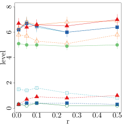
n=25𝑛25n=25 n=50𝑛50n=50 n=100𝑛100n=100
Refer to caption Refer to caption Refer to caption
Figure 1: Estimated test levels in percentage under 0subscript0\mathcal{H}_{0} for varying magnitudes of common non null coefficients, based upon 1000 simulations. Bonferroni calibration in dotted lines, calibration by permutation in plain lines. Blue squares represent the suggested test T𝒮^subscriptsuperscript𝑇^𝒮T^{*}_{\widehat{\mathcal{S}}}, red triangles stand for the Fisher test T𝒮^,Fishersubscriptsuperscript𝑇Fisher^𝒮T^{*,\mathrm{Fisher}}_{\widehat{\mathcal{S}}}. The deterministic collection 𝒮1subscript𝒮1{\mathcal{S}}_{1} is drawn in empty points, while the data-driven collection 𝒮^Lassosubscript^𝒮Lasso{\widehat{\mathcal{S}}_{\text{Lasso}}} is in plain points. Green circles represent the DiffRegr procedure, respectively plain and empty for single-splitting and multi-splitting.
Refer to caption
Figure 2: Legend of the procedures under study
Power decay GGM
Refer to caption Refer to caption
Figure 3: Estimated test levels in percentage under 0subscript0\mathcal{H}_{0} for varying magnitudes of common non null coefficients, based upon 1000 simulations, under power decay and GGM correlation structures when n=50𝑛50n=50. Bonferroni calibration in dotted lines, calibration by permutation in plain lines. Blue squares represent the suggested test T𝒮^subscriptsuperscript𝑇^𝒮T^{*}_{\widehat{\mathcal{S}}}, red triangles stand for the Fisher test T𝒮^,Fishersubscriptsuperscript𝑇Fisher^𝒮T^{*,\mathrm{Fisher}}_{\widehat{\mathcal{S}}}. The deterministic collection 𝒮1subscript𝒮1{\mathcal{S}}_{1} is drawn in empty points, while the data-driven collection 𝒮^Lassosubscript^𝒮Lasso{\widehat{\mathcal{S}}_{\text{Lasso}}} is in plain points. Green circles represent the DiffRegr procedure, respectively plain and empty for single-splitting and multi-splitting.
Power Analysis.

We do not investigate the power of the Bonferroni-based procedures T𝒮^Bsubscriptsuperscript𝑇𝐵^𝒮T^{B}_{\widehat{{\mathcal{S}}}} and T𝒮^B,Fishersubscriptsuperscript𝑇𝐵Fisher^𝒮T^{B,\mathrm{Fisher}}_{\widehat{{\mathcal{S}}}} as they have been shown to be too conservative in the above Type I error analysis. Figure 4 represents power performances for the test T𝒮^Psubscriptsuperscript𝑇𝑃^𝒮T^{P}_{\widehat{\mathcal{S}}} and the usual likelihood ratio test T𝒮^P,Fishersubscriptsuperscript𝑇𝑃Fisher^𝒮T^{P,\mathrm{Fisher}}_{\widehat{\mathcal{S}}} combined with either 𝒮1subscript𝒮1{\mathcal{S}}_{1} or 𝒮^Lassosubscript^𝒮Lasso{\widehat{\mathcal{S}}_{\text{Lasso}}} test collections using a calibration by permutation under an orthogonal covariance matrix ΣΣ\Sigma, as well as power performance for the DiffRegr procedure. Figure 5 represents equivalent results for power decay and GGM covariance structures when n=50𝑛50n=50.

In the absence of common coefficients (scenarios 1 and 2), the test T𝒮^Psubscriptsuperscript𝑇𝑃^𝒮T^{P}_{\widehat{\mathcal{S}}} reaches 100% power from very low signal magnitudes and small sample sizes. Compared to the test based on usual likelihood ratio statistics, which does not reach more than 40% power when n=25𝑛25n=25 given the signal magnitudes under consideration, the suggested statistics proves itself extremely efficient. Under these settings as well, any subset of size 1 containing one of the variables activated in only β(2)superscript𝛽2\beta^{(2)} can suffice to reject the null, which is why collection 𝒮1subscript𝒮1{\mathcal{S}}_{1} performs actually very well when associated with (FS,V,FS,1,FS,2)subscript𝐹𝑆𝑉subscript𝐹𝑆1subscript𝐹𝑆2(F_{S,V},F_{S,1},F_{S,2}) and not so badly when associated with FiSsubscriptFi𝑆\mathrm{Fi}_{S}.

However, in more complex settings 3 and 4, where larger subsets are required to correct for strong and numerous common effects, subset collection 𝒮^Lassosubscript^𝒮Lasso{\widehat{\mathcal{S}}_{\text{Lasso}}} yields a higher power than the collection 𝒮1subscript𝒮1{\mathcal{S}}_{1}.

For small n𝑛n, the test T𝒮^LassoPsubscriptsuperscript𝑇𝑃subscript^𝒮LassoT^{P}_{{\widehat{\mathcal{S}}_{\text{Lasso}}}} outperforms the procedure DiffRegr, whose limitation likely stems from the half sampling step. This limitation of sample splitting approaches has already been noticed by [40]. However, for n=100𝑛100n=100 the procedure DiffRegr performs better than our procedure in the highly challenging setting 4.

Settings n=25𝑛25n=25 n=50𝑛50n=50 n=100𝑛100n=100
1. Refer to caption Refer to caption Refer to caption Refer to caption
2. Refer to caption Refer to caption Refer to caption Refer to caption
3. Refer to caption Refer to caption Refer to caption Refer to caption
4. Refer to caption Refer to caption Refer to caption Refer to caption
Figure 4: Power (in percentage) as a function of signal magnitude parameter r𝑟r for various sparsity pattern under the assumption of uncorrelated designs Σ(1)=Σ(2)=IpsuperscriptΣ1superscriptΣ2subscript𝐼𝑝\Sigma^{(1)}=\Sigma^{(2)}=I_{p}. Results for the suggested test T𝒮^Psubscriptsuperscript𝑇𝑃^𝒮T^{P}_{\widehat{\mathcal{S}}} and the test T𝒮^P,Fishersubscriptsuperscript𝑇𝑃Fisher^𝒮T^{P,\mathrm{Fisher}}_{\widehat{\mathcal{S}}}, combined with 𝒮1subscript𝒮1{\mathcal{S}}_{1} or 𝒮^Lassosubscript^𝒮Lasso{\widehat{\mathcal{S}}_{\text{Lasso}}} test collections. Blue squares represent the suggested test T𝒮^Psubscriptsuperscript𝑇𝑃^𝒮T^{P}_{\widehat{\mathcal{S}}}, red triangles stand for the Fisher test T𝒮^P,Fishersubscriptsuperscript𝑇𝑃Fisher^𝒮T^{P,\mathrm{Fisher}}_{\widehat{\mathcal{S}}}. The deterministic collection 𝒮1subscript𝒮1{\mathcal{S}}_{1} is drawn in empty points, while the data-driven collection 𝒮^Lassosubscript^𝒮Lasso{\widehat{\mathcal{S}}_{\text{Lasso}}} is in plain points. Results for the DiffRegr procedure are represented by green circles, respectively plain and empty for single-splitting and multi-splitting approaches.

Figure 5 provide similar results under respectively power decay correlated designs and GGM-like correlated designs for a sample size of n=50𝑛50n=50, leading to similar conclusions as in the uncorrelated case.

Settings Power decay GGM
1. Refer to caption Refer to caption Refer to caption
2. Refer to caption Refer to caption Refer to caption
3. Refer to caption Refer to caption Refer to caption
4. Refer to caption Refer to caption Refer to caption
Figure 5: Power (in percentage) as a function of signal magnitude parameter r𝑟r for various sparsity patterns under power decay and GGM correlated designs, at n=50𝑛50n=50 observations. Results for the suggested test T𝒮^Psubscriptsuperscript𝑇𝑃^𝒮T^{P}_{\widehat{\mathcal{S}}} and the test T𝒮^P,Fishersubscriptsuperscript𝑇𝑃Fisher^𝒮T^{P,\mathrm{Fisher}}_{\widehat{\mathcal{S}}}, combined with 𝒮1subscript𝒮1{\mathcal{S}}_{1} or 𝒮^Lassosubscript^𝒮Lasso{\widehat{\mathcal{S}}_{\text{Lasso}}} test collections and a calibration by permutation. Blue squares represent the suggested test T𝒮^Psubscriptsuperscript𝑇𝑃^𝒮T^{P}_{\widehat{\mathcal{S}}}, red triangles stand for the Fisher test T𝒮^P,Fishersubscriptsuperscript𝑇𝑃Fisher^𝒮T^{P,\mathrm{Fisher}}_{\widehat{\mathcal{S}}}. The deterministic collection 𝒮1subscript𝒮1{\mathcal{S}}_{1} is drawn in empty points, while the data-driven collection 𝒮^Lassosubscript^𝒮Lasso{\widehat{\mathcal{S}}_{\text{Lasso}}} is in plain points. Results for the DiffRegr procedure are represented by green circles, respectively plain and empty for single-splitting and multi-splitting approaches.

6 Application to GGM

The following section explicits the extension of the two-sample linear regression testing framework to the two-sample Gaussian graphical model testing framework. We describe the tools and guidelines for a correct interpretation of the results and illustrate the approach on a typical two-sample transcriptomic data-set.

6.1 How to Apply this Strategy to GGM Testing

Neighborhood Selection Approach

The procedure developed in Section 2 can be adapted to the case of Gaussian graphical models as in [45]. We quickly recall why estimation of the Gaussian graphical model amounts to the estimation of p𝑝p independent linear regressions when adopting a neighborhood selection approach [32].

Consider two Gaussian random vectors Z(1)𝒩(0,[Ω(1)]1)similar-tosuperscript𝑍1𝒩0superscriptdelimited-[]superscriptΩ11{Z}^{(1)}\sim\mathcal{N}(0,\left[\Omega^{(1)}\right]^{-1}) and Z(2)𝒩(0,[Ω(2)]1)similar-tosuperscript𝑍2𝒩0superscriptdelimited-[]superscriptΩ21{Z}^{(2)}\sim\mathcal{N}(0,\left[\Omega^{(2)}\right]^{-1}). Their respective conditional independence structures are represented by the graphs 𝒢(1)superscript𝒢1\mathcal{G}^{(1)} and 𝒢(2)superscript𝒢2\mathcal{G}^{(2)}, which consist of a common set of nodes Γ={1,,p}Γ1𝑝\Gamma=\{1,\dots,p\} and their respective sets of edges (1)superscript1\mathcal{E}^{(1)} and (2)superscript2\mathcal{E}^{(2)}. When speaking of gene regulation networks, each node represents a gene, and edges between genes are indicative of potential regulations. In contrast with gene co-expression networks, edges in Gaussian graphical models do not reflect correlations but partial correlations between gene expression profiles.

Formally, an edge (i,j)𝑖𝑗(i,j) belongs to the edge set (1)superscript1\mathcal{E}^{(1)} (resp. (2)superscript2\mathcal{E}^{(2)}) if Zi(1)subscriptsuperscript𝑍1𝑖Z^{(1)}_{i} (resp. Zi(2)subscriptsuperscript𝑍2𝑖Z^{(2)}_{i}) is independent from Zj(1)subscriptsuperscript𝑍1𝑗Z^{(1)}_{j} (resp. Zj(2)subscriptsuperscript𝑍2𝑗Z^{(2)}_{j}) conditional on all other variables Z\i,j(1)subscriptsuperscript𝑍1\absent𝑖𝑗Z^{(1)}_{\backslash i,j} (resp. Z\i,j(2)subscriptsuperscript𝑍2\absent𝑖𝑗Z^{(2)}_{\backslash i,j}). When the precision matrix Ω(k)superscriptΩ𝑘\Omega^{(k)} is nonsingular, the edges are characterized by its non zero entries.

The idea of neighborhood selection is to circumvent the intricate issue of estimating the precision matrix by recovering the sets of edges neighborhood by neighborhood, through the conditional distribution of Zi(k)subscriptsuperscript𝑍𝑘𝑖Z^{(k)}_{i} given all remaining variables Z\i(k)subscriptsuperscript𝑍𝑘\absent𝑖Z^{(k)}_{\backslash i}. Indeed, this distribution is again a Gaussian distribution, whose mean is a linear combination of Z\i(k)subscriptsuperscript𝑍𝑘\absent𝑖Z^{(k)}_{\backslash i} while its variance is independent from Z\i(k)subscriptsuperscript𝑍𝑘\absent𝑖Z^{(k)}_{\backslash i}. Hence, Zi(k)subscriptsuperscript𝑍𝑘𝑖Z^{(k)}_{i} can be decomposed into the following linear regression:

Zi(k)=jiZj(k)βij(k)+εi(k)=Z\i(k)βi(k)+εi(k),subscriptsuperscript𝑍𝑘𝑖subscript𝑗𝑖superscriptsubscript𝑍𝑗𝑘superscriptsubscript𝛽𝑖𝑗𝑘superscriptsubscript𝜀𝑖𝑘superscriptsubscript𝑍\absent𝑖𝑘superscriptsubscript𝛽𝑖𝑘superscriptsubscript𝜀𝑖𝑘Z^{(k)}_{i}=\sum_{j\neq i}Z_{j}^{(k)}\beta_{ij}^{(k)}+\varepsilon_{i}^{(k)}=Z_{\backslash i}^{(k)}\beta_{i}^{(k)}+\varepsilon_{i}^{(k)}\ , (43)

where βij(k)=Ωij(k)/Ωii(k)superscriptsubscript𝛽𝑖𝑗𝑘superscriptsubscriptΩ𝑖𝑗𝑘superscriptsubscriptΩ𝑖𝑖𝑘\beta_{ij}^{(k)}=-\Omega_{ij}^{(k)}/\Omega_{ii}^{(k)} and Var[εi(k)]=(Ωii(k))1Vardelimited-[]superscriptsubscript𝜀𝑖𝑘superscriptsuperscriptsubscriptΩ𝑖𝑖𝑘1\mbox{Var}[\varepsilon_{i}^{(k)}]=(\Omega_{ii}^{(k)})^{-1}.

Given an n1subscript𝑛1n_{1}-sample of Z(1)superscript𝑍1Z^{(1)} and an n2subscript𝑛2n_{2}-sample of Z(2)superscript𝑍2Z^{(2)}, we recall that our objective is to test as formalized in (4)

0G:Ω(1)=Ω(2) versus 1G:Ω(1)Ω(2).:subscriptsuperscript𝐺0superscriptΩ1superscriptΩ2 versus subscriptsuperscript𝐺1:superscriptΩ1superscriptΩ2\mathcal{H}^{G}_{0}:\ \Omega^{(1)}=\Omega^{(2)}\quad\text{ versus }\quad\mathcal{H}^{G}_{1}:\ \Omega^{(1)}\neq\Omega^{(2)}\ .

As a result of Equation (43), testing for the equality of the matrix rows Ωi.(1)=Ωi.(2)subscriptsuperscriptΩ1𝑖subscriptsuperscriptΩ2𝑖\Omega^{(1)}_{i.}=\Omega^{(2)}_{i.} is equivalent to testing for βi(1)=βi(2)superscriptsubscript𝛽𝑖1superscriptsubscript𝛽𝑖2\beta_{i}^{(1)}=\beta_{i}^{(2)} and Var[εi(1)]=Var[εi(2)]Vardelimited-[]superscriptsubscript𝜀𝑖1Vardelimited-[]superscriptsubscript𝜀𝑖2\mbox{Var}[\varepsilon_{i}^{(1)}]=\mbox{Var}[\varepsilon_{i}^{(2)}]. Denote by Σ\i(k)subscriptsuperscriptΣ𝑘\absent𝑖\Sigma^{(k)}_{\backslash i} the covariance of Z\i(k)subscriptsuperscript𝑍𝑘\absent𝑖Z^{(k)}_{\backslash i}. Under the null 0Gsubscriptsuperscript𝐺0\mathcal{H}^{G}_{0}, we have that for any i𝑖i, Σ\i(1)=Σ\i(2)subscriptsuperscriptΣ1\absent𝑖subscriptsuperscriptΣ2\absent𝑖\Sigma^{(1)}_{\backslash i}=\Sigma^{(2)}_{\backslash i}. Consequently, we can translate the GGM hypotheses given in Equation (4) into a conjunction of two-sample linear regression tests:

0G::subscriptsuperscript𝐺0absent\displaystyle\mathcal{H}^{G}_{0}: i[βi(1)=βi(2),Ωii(1)=Ωii(2),Σ\i(1)=Σ\i(2)]subscript𝑖delimited-[]formulae-sequencesuperscriptsubscript𝛽𝑖1superscriptsubscript𝛽𝑖2formulae-sequencesuperscriptsubscriptΩ𝑖𝑖1superscriptsubscriptΩ𝑖𝑖2subscriptsuperscriptΣ1\absent𝑖subscriptsuperscriptΣ2\absent𝑖\displaystyle\ \bigcap_{i}\left[\beta_{i}^{(1)}=\beta_{i}^{(2)},\ \Omega_{ii}^{(1)}=\Omega_{ii}^{(2)},\ \Sigma^{(1)}_{\backslash i}=\Sigma^{(2)}_{\backslash i}\right] (44)
1G::subscriptsuperscript𝐺1absent\displaystyle\mathcal{H}^{G}_{1}: i[βi(1)βi(2)][Ωii(1)Ωii(2)].subscript𝑖delimited-[]superscriptsubscript𝛽𝑖1superscriptsubscript𝛽𝑖2delimited-[]superscriptsubscriptΩ𝑖𝑖1superscriptsubscriptΩ𝑖𝑖2\displaystyle\ \bigcup_{i}\left[\beta_{i}^{(1)}\neq\beta_{i}^{(2)}\right]\cup\left[\Omega_{ii}^{(1)}\neq\Omega_{ii}^{(2)}\right]\ .

Concretely, we apply the previous two-sample linear regression model with 𝐗(1)=𝐙,\i(1)\mathbf{X}^{(1)}=\mathbf{Z}^{(1)}_{,\backslash i},𝐗(2)=𝐙,\i(2)\mathbf{X}^{(2)}=\mathbf{Z}^{(2)}_{,\backslash i}, 𝐘(1)=𝐙,i(1)\mathbf{Y}^{(1)}=\mathbf{Z}^{(1)}_{,i}, and 𝐘(2)=𝐙,i(2)\mathbf{Y}^{(2)}=\mathbf{Z}^{(2)}_{,i} for every gene i𝑖i and combine multiple neighborhood tests using a Bonferroni calibration as presented in Algorithm 5. The equality of σ(k)superscript𝜎𝑘\sigma^{(k)}’s in 0subscript0\mathcal{H}_{0} models the equality of Ωii(k)superscriptsubscriptΩ𝑖𝑖𝑘\Omega_{ii}^{(k)}’s in 0Gsuperscriptsubscript0𝐺\mathcal{H}_{0}^{G} while the equality of Σ(k)superscriptΣ𝑘\Sigma^{(k)}’s accounts for the equality of Σ\i(k)superscriptsubscriptΣ\absent𝑖𝑘\Sigma_{\backslash i}^{(k)}’s.

Algorithm 5 Gaussian Graphical Model Testing Strategy
Data 𝐙(1)superscript𝐙1\mathbf{Z}^{(1)},𝐙(2)superscript𝐙2\mathbf{Z}^{(2)}, maximum model dimension Dmaxsubscript𝐷𝑚𝑎𝑥D_{max} and desired level α𝛼\alpha
for each gene i=1,,p𝑖1𝑝i=1,\dots,p do
     procedure Neighborhood Test
         Define 𝐗(1)=𝐙,\i(1),𝐗(2)=𝐙,\i(2)\mathbf{X}^{(1)}=\mathbf{Z}^{(1)}_{,\backslash i},\quad\mathbf{X}^{(2)}=\mathbf{Z}^{(2)}_{,\backslash i}
         Define 𝐘(1)=𝐙,i(1),𝐘(2)=𝐙,i(2)\mathbf{Y}^{(1)}=\mathbf{Z}^{(1)}_{,i},\quad\mathbf{Y}^{(2)}=\mathbf{Z}^{(2)}_{,i}
         Apply the Adaptive Testing Strategy of Algorithm 1 to 𝐗(1)superscript𝐗1\mathbf{X}^{(1)},𝐗(2)superscript𝐗2\mathbf{X}^{(2)},𝐘(1)superscript𝐘1\mathbf{Y}^{(1)},𝐘(2)superscript𝐘2\mathbf{Y}^{(2)}
     end procedure
end for
Reject the global null hypothesis if at least one Neighborhood Test is rejected at level α/p𝛼𝑝\alpha/p
Interpretation.

Because we need Ωii(1)=Ωii(2)superscriptsubscriptΩ𝑖𝑖1superscriptsubscriptΩ𝑖𝑖2\Omega_{ii}^{(1)}=\Omega_{ii}^{(2)} and Σ\i(1)=Σ\i(2)superscriptsubscriptΣ\absent𝑖1superscriptsubscriptΣ\absent𝑖2\Sigma_{\backslash i}^{(1)}=\Sigma_{\backslash i}^{(2)} for every neighborhood in the two-sample GGM null hypothesis 0Nsubscriptsuperscript𝑁0\mathcal{H}^{N}_{0} (44), the assumptions that σ(1)=σ(2)superscript𝜎1superscript𝜎2\sigma^{(1)}=\sigma^{(2)} and Σ(1)=Σ(2)superscriptΣ1superscriptΣ2\Sigma^{(1)}=\Sigma^{(2)} in the two-sample linear regression null hypothesis 0subscript0\mathcal{H}_{0} (3) are crucial for each neighorbood test to be interpreted correctly. As a result, only the global test can be strictly speaking interpreted in a statistically correct sense.

However in practice, when the global null hypothesis is rejected, our construction of neighborhood tests provides helpful clues on the location of disruptive regulations. In particular, for each rejected neighorhood test i𝑖i, one can keep track of the rejected model SRisuperscriptsubscript𝑆𝑅𝑖S_{R}^{i}, retaining sensible information on which particular regulations are most likely altered between samples.

6.2 Illustration on Real Transcriptomic Breast Cancer Data

We apply this strategy to the full (training and validation) breast cancer dataset studied by [21] and [35], whose training subset was originally published in [37]. The full dataset consists of microarray gene expression profiles from 133 patients with stage I-III breast cancer undergoing preoperative chemotherapy. A majority of patients (n=99) presented residual disease (RD), while 34 patients demonstrated a pathologic complete response (pCR). The common objective of [21] and [35] was to develop a predictor of complete response to treatment from gene expression profiling. In particular, [21] identified an optimal predictive subset of 30 probes, mapping to 26 distinct genes.

[2] inferred Gaussian graphical models among those 26 genes on each patient class using weighted neighborhood selection. The corresponding graphs of conditional dependencies for medium regularization are presented in Figure 6. Those two graphs happen to differ dramatically from one another. The question we tackle is whether those differences remain when taking into account estimation uncertainties.

Pathologic Complete Response (pCR) Residual Disease (RD)
Refer to caption Refer to caption
Figure 6: Graphs of conditional dependencies among the 26 genes selected by [21] on patients with pathologic complete response or residual disease with medium regularization as presented in Figure 3 of [2].

We run for each of the p=26𝑝26p=26 genes a neighborhood test TS^LassoPsuperscriptsubscript𝑇subscript^𝑆𝐿𝑎𝑠𝑠𝑜𝑃T_{\hat{S}_{Lasso}}^{P} at level 0.05/260.05260.05/26. We associate to each neighborhood test the empirical p-value defined in 25 that has to be be compared to α/p𝛼𝑝\alpha/p.

Most of the graph estimation methods proposed in the literature, such as the procedure of [2] leading to Figure 6, rely on the assumption that observations are i.i.d. Yet the training and validation datasets have been collected and analysed separately by two different clinical centers. We therefore start by checking whether the pooled sample can be considered as homogeneous. Within each group of patients (RD and pCR), we lead a test for the homogeneity of Gaussian graphical models between the training and validation subsets.

Within pCR patients (3), two neighborhood tests corresponding to CA12 and PDGFRA are rejected at level 0.05/260.05260.05/26. Within RD patients (4), half of the neighborhoods happen to differ significantly between the training and validation datasets. Genes CA12 and JMJD2B are responsible for the rejection of respectively seven and six neighborhoods.

AMFR BB_S4 BECNI BTG3 CA12 CTNND2 E2F3
decision 0 0 0 0 1 0 0
pempiricalsuperscript𝑝𝑒𝑚𝑝𝑖𝑟𝑖𝑐𝑎𝑙p^{empirical} 0.0492 0.0072 0.1972 1 0.0018 0.0100 0.1080
ERBB4 FGFRIOP FLJ10916 FLJI2650 GAMT GFRAI IGFBP4
decision 0 0 0 0 0 0 0
pempiricalsuperscript𝑝𝑒𝑚𝑝𝑖𝑟𝑖𝑐𝑎𝑙p^{empirical} 0.5610 0.0242 0.2542 0.0312 0.1158 0.5318 0.0458
JMJD2B KIA1467 MAPT MBTP_SI MELK METRN PDGFRA
decision 0 0 0 0 0 0 1
pempiricalsuperscript𝑝𝑒𝑚𝑝𝑖𝑟𝑖𝑐𝑎𝑙p^{empirical} 0.0128 0.0272 0.0178 0.0062 0.5602 1 0.0012
RAMPI RRM2 SCUBE2 THRAP2 ZNF552
decision 0 0 0 0 0
pempiricalsuperscript𝑝𝑒𝑚𝑝𝑖𝑟𝑖𝑐𝑎𝑙p^{empirical} 0.0444 0.0022 0.2372 0.0228 0.0028
Table 3: Homogeneity test between training and test samples among pCR patients. Summary of test decisions after Bonferroni multiple testing correction and empirical p-values for each neighborhood test as defined in Section 3.4.
AMFR BB_S4 BECNI BTG3 CA12 CTNND2 E2F3
decision 0 1 1 0 1 0 0
pempiricalsuperscript𝑝𝑒𝑚𝑝𝑖𝑟𝑖𝑐𝑎𝑙p^{empirical} 0.0046 <<0.0001 <<0.0001 0.0202 <<0.0001 0.0684 0.0428
ERBB4 FGFRIOP FLJ10916 FLJI2650 GAMT GFRAI IGFBP4
decision 0 1 1 1 1 0 0
pempiricalsuperscript𝑝𝑒𝑚𝑝𝑖𝑟𝑖𝑐𝑎𝑙p^{empirical} 0.26 <<0.0001 <<0.0001 0.002 <<0.0001 0.3606 0.389
JMJD2B KIA1467 MAPT MBTP_SI MELK METRN PDGFRA
decision 1 1 0 1 0 0 1
pempiricalsuperscript𝑝𝑒𝑚𝑝𝑖𝑟𝑖𝑐𝑎𝑙p^{empirical} <<0.0001 2e-04 0.006 6e-04 0.1556 0.1054 <<0.0001
RAMPI RRM2 SCUBE2 THRAP2 ZNF552
decision 0 0 0 1 1
pempiricalsuperscript𝑝𝑒𝑚𝑝𝑖𝑟𝑖𝑐𝑎𝑙p^{empirical} 0.2288 0.2988 0.3552 <<0.0001 <<0.0001
Table 4: Homogeneity test between training and test samples among RD patients. Summary of test decisions after Bonferroni multiple testing correction and empirical p-values for each neighborhood test as defined in Section 3.4

Because of these surprisingly significant divergences between training and validation subsets, we restrict the subsequent analysis to the training set (n=82 patients, among which 61 RD and 21 pCR patients).

To roughly check that we got rid of the underlying heterogeneity, we create an artificial dataset under H0subscript𝐻0H_{0} by permutation of the patients, regardless of their class. No neighborhood test is rejected at a level corrected for multiple testing. We also cut the group of patients with residual disease artificially in half. When testing for the difference between the two halves, no significant heterogeneity remains, whatever the neighborhood.

Within the training set, the comparison of Gaussial graphical structures between pCR and RD patients leads to the rejection of all neighborhood tests after Bonferroni correction for multiple testing of the 26 neighborhoods, as summarized in Table 5. RRM2, MAPT and MELK genes appear as responsible for the rejection of respectively nine, nine and four of these neighborhood tests. Quite interestingly, these three genes have all been described in clinical literature as new promising drug targets. [20] exhibited inhibitors of RRM2 expression, which reduced in vitro and in vivo cell proliferation. [38] led functional biology experiments validating the relationship between MAPT expression levels and response to therapy, suggesting to inhibit its expression to increase sensivity to treatment. More recently, [13] developed a therapeutic candidate inhibiting MELK expression that was proved to suppress the growth of tumour-initiating cells in mice with various cancer types, including breast cancer.

AMFR BB_S4 BECNI BTG3 CA12 CTNND2 E2F3
decision 1 1 1 1 1 1 1
pempiricalsuperscript𝑝𝑒𝑚𝑝𝑖𝑟𝑖𝑐𝑎𝑙p^{empirical} << 0.0001 <<0.0001 4e-04 <<0.0001 2e-04 <<0.0001 <<0.0001
rejected model RRM2 RRM2 MAPT MAPT MAPT RRM2 MAPT
ERBB4 FGFRIOP FLJ10916 FLJI2650 GAMT GFRAI IGFBP4
decision 1 1 1 1 1 1 1
pempiricalsuperscript𝑝𝑒𝑚𝑝𝑖𝑟𝑖𝑐𝑎𝑙p^{empirical} <<0.0001 4e-04 4e-04 <<0.0001 <<0.0001 <<0.0001 <<0.0001
rejected model MELK MAPT RRM2 MAPT RRM2 BTG3 MELK
JMJD2B KIA1467 MAPT MBTP_SI MELK METRN PDGFRA
decision 1 1 1 1 1 1 1
pempiricalsuperscript𝑝𝑒𝑚𝑝𝑖𝑟𝑖𝑐𝑎𝑙p^{empirical} <<0.0001 <<0.0001 <<0.0001 <<0.0001 <<0.0001 <<0.0001 <<0.0001
rejected model MAPT MELK RRM2 E2F3 MAPT MELK RRM2
RAMPI RRM2 SCUBE2 THRAP2 ZNF552
decision 1 1 1 1 1
pempiricalsuperscript𝑝𝑒𝑚𝑝𝑖𝑟𝑖𝑐𝑎𝑙p^{empirical} <<0.0001 <<0.0001 <<0.0001 <<0.0001 2e-04
rejected model RRM2 MAPT BTG3 E2F3 RRM2
Table 5: Summary of neighborhood tests between RD and pCR patients within the training set (n=82). Decision is made at level 0.05/260.05260.05/26 to correct for multiple testing. The empirical p𝑝p-value and the rejected model are defined in Section 3.4.

For comprehensiveness, we add that similar analysis of the validation set (n=51 patients, among which 38 RD and 13 pCR patients) leads to the identification of only 9 significantly altered neighborhoods between pCR and RD patients 6. This difference in the number of significantly altered neighborhoods can be explained by the reduced size of the sample. Yet, genes responsible for the rejection of the tests differ from those identified on the training set. In particular, five of the significant tests are rejected because of SCUBE2, which has been recently recognised as a novel tumor suppressor gene [28].

AMFR BB_S4 BECNI BTG3 CA12 CTNND2 E2F3
decision 0 0 0 1 0 0 1
pempiricalsuperscript𝑝𝑒𝑚𝑝𝑖𝑟𝑖𝑐𝑎𝑙p^{empirical} 0.0024 0.0028 0.0048 0.0018 0.0028 0.0082 <<0.0001
rejected model - - - SCUBE2 - - METRN
ERBB4 FGFRIOP FLJ10916 FLJI2650 GAMT GFRAI IGFBP4
decision 1 0 1 0 0 1 1
pempiricalsuperscript𝑝𝑒𝑚𝑝𝑖𝑟𝑖𝑐𝑎𝑙p^{empirical} 0.0014 0.0072 8e-04 0.0142 0.0046 8e-04 2e-04
rejected model SCUBE2 - SCUBE2 - - E2F3 SCUBE2
JMJD2B KIA1467 MAPT MBTP_SI MELK METRN PDGFRA
decision 0 1 0 0 0 1 0
pempiricalsuperscript𝑝𝑒𝑚𝑝𝑖𝑟𝑖𝑐𝑎𝑙p^{empirical} 0.0054 0.0018 0.0032 0.0078 0.0036 4e-04 0.0104
rejected model - SCUBE2 - - - E2F3 -
RAMPI RRM2 SCUBE2 THRAP2 ZNF552
decision 0 0 1 0 0
pempiricalsuperscript𝑝𝑒𝑚𝑝𝑖𝑟𝑖𝑐𝑎𝑙p^{empirical} 0.0056 0.0034 2e-04 0.0024 0.006
rejected model - - FLJ10916 - -
Table 6: Summary of neighborhood tests between RD and pCR patients within the validation set (n=51). Decision is made at level 0.05/260.05260.05/26 to correct for multiple testing. The empirical p𝑝p-value and the rejected model are defined in Section 3.4.

7 Discussion

Design hypotheses.

In this work, we have made two main assumptions on the design matrices:

  1. (i)

    The design matrices 𝐗(1)superscript𝐗1{\bf X}^{(1)} and 𝐗(2)superscript𝐗2{\bf X}^{(2)} are random.

  2. (ii)

    Under the null hypothesis (3), we further suppose that the population covariances Σ(1)superscriptΣ1\Sigma^{(1)} and Σ(2)superscriptΣ2\Sigma^{(2)} are equal.

Although this setting is particularly suited to consider the two-sample GGM testing (Section 6), one may wonder whether one can circumvent these two restrictions. We doubt that this is possible without making the testing problem much more difficult.

First, the formulation (3) allows the null hypothesis to be interpreted as a relevant intermediary case between two extreme fixed design settings: design equality (𝐗(1)=𝐗(2)superscript𝐗1superscript𝐗2{\bf X}^{(1)}={\bf X}^{(2)}) and arbitrary different design (𝐗(1)𝐗(2)superscript𝐗1superscript𝐗2{\bf X}^{(1)}\neq{\bf X}^{(2)}). In the first case, the two-sample problem amounts to a one-sample problem by considering 𝐘~=𝐘(1)𝐘(2)~𝐘superscript𝐘1superscript𝐘2\tilde{\bf Y}={\bf Y}^{(1)}-{\bf Y}^{(2)} and it has therefore already been thoroughly studied. The second case is on the contrary extremely difficult as illustrated by the proposition below.

Proposition 7.1.

Consider the design matrices 𝐗(1)superscript𝐗1{\bf X}^{(1)} and 𝐗(2)superscript𝐗2{\bf X}^{(2)} as fixed and assume that σ(1)=σ(2)=1superscript𝜎1superscript𝜎21\sigma^{(1)}=\sigma^{(2)}=1. If the (n1+n2)×psubscript𝑛1subscript𝑛2𝑝(n_{1}+n_{2})\times p matrix formed by 𝐗(1)superscript𝐗1{\bf X}^{(1)} and 𝐗(2)superscript𝐗2{\bf X}^{(2)} has rank n1+n2subscript𝑛1subscript𝑛2n_{1}+n_{2}, then any test T𝑇T of β(1)=β(2)superscript𝛽1superscript𝛽2\beta^{(1)}=\beta^{(2)} vs β(1)β(2)superscript𝛽1superscript𝛽2\beta^{(1)}\neq\beta^{(2)} based on the data (𝐘,𝐗)𝐘𝐗({\bf Y},{\bf X}) satisfies:

supβpβ,β[T=1]+infβ(1)β(2)pβ(1),β(2)[T=0]1,subscriptsupremum𝛽superscript𝑝subscript𝛽𝛽delimited-[]𝑇1subscriptinfimumsuperscript𝛽1superscript𝛽2superscript𝑝subscriptsuperscript𝛽1superscript𝛽2delimited-[]𝑇01\sup_{\beta\in\mathbb{R}^{p}}\mathbb{P}_{\beta,\beta}[T=1]+\inf_{\beta^{(1)}\neq\beta^{(2)}\in\mathbb{R}^{p}}\mathbb{P}_{\beta^{(1)},\beta^{(2)}}[T=0]\geq 1\ ,

where β(1),β(2)(.)\mathbb{P}_{\beta^{(1)},\beta^{(2)}}(.) denotes the distribution of (𝐘(1),𝐘(2))superscript𝐘1superscript𝐘2({\bf Y}^{(1)},{\bf Y}^{(2)}). In other words, any level-α𝛼\alpha test T𝑇T has a type II error larger than 1α1𝛼1-\alpha, and this uniformly over β(1)superscript𝛽1\beta^{(1)} and β(2)superscript𝛽2\beta^{(2)}. Consequently, any test in this setting cannot perform better than complete random guess.

Furthermore, if Σ(1)Σ(2)superscriptΣ1superscriptΣ2\Sigma^{(1)}\neq\Sigma^{(2)} is allowed in the null (3), then the two-sample testing problem becomes much more difficult in the sense that it is impossible to reformulate the null hypothesis into a conjonction of low-dimensional hypotheses as done in Lemma 2.1. Indeed, consider the following toy example: σ(1)=σ(2)=1superscript𝜎1superscript𝜎21\sigma^{(1)}=\sigma^{(2)}=1, β(1)=β(2)=(a,0,0,)Tsuperscript𝛽1superscript𝛽2superscript𝑎00𝑇\beta^{(1)}=\beta^{(2)}=(a,0,0,\ldots)^{T} for some a>0𝑎0a>0, Σ(1)=IpsuperscriptΣ1subscript𝐼𝑝\Sigma^{(1)}=I_{p} and Σ(2)=(ρ+𝟏i=j)1i,jpsuperscriptΣ2subscript𝜌subscript1𝑖𝑗formulae-sequence1𝑖𝑗𝑝\Sigma^{(2)}=(\rho+\mathbf{1}_{i=j})_{1\leq i,j\leq p} for some ρ>0𝜌0\rho>0. Then, for any subset S𝑆S that does not contain the first component, the parameters βS(1)subscriptsuperscript𝛽1𝑆\beta^{(1)}_{S} and βS(2)subscriptsuperscript𝛽2𝑆\beta^{(2)}_{S} are different. Consequently, βS(1)βS(2)subscriptsuperscript𝛽1𝑆subscriptsuperscript𝛽2𝑆\beta^{(1)}_{S}\neq\beta^{(2)}_{S} does not imply that β(1)β(2)superscript𝛽1superscript𝛽2\beta^{(1)}\neq\beta^{(2)} and one should not rule out the parameter equality hypothesis relying on some low-dimensional regressions.

Comparison with related work [40, 41]

Städler and Mukherjee propose a very general approach to high-dimensional two-sample testing, being applicable to a wide range of models. In particular this approach allows for the direct comparison of two-sample Gaussian graphical models without adopting a neighborhood selection approach. This avoids the burden of multiple neighborhood linear regression and the multiple testing correction which follows.

Because they estimate the supports of sample-specific estimators and joint estimator separately in the screening step, they resort to an elegant estimation of the p𝑝p-values for the non-nested likelihood ratio test in the cleaning step. Yet, they do not provide any theoretical controls on type I error rate or power for their overall testing strategy.

Finally, as it appears in the numerical experiments, their approach is based on half-sampling and can thus suffer from an acute reduction of power on small samples. On the bright side, the multi-split procedure shows stable results and performs well even in difficult scenarios as soon as n𝑛n is sufficiently large.

Non asymptotic bounds and constants.

In the spirit of [6], our type II error analysis is completely non-asymptotic. However, the numerical constants involved in the bounds are clearly not optimal. Another line of work initiated by [15] considers an asymptotic but high-dimensional framework and aims to provide detection rates with optimal constants. For instance [3, 22] have derived such results in the one-sample high-dimensional linear regression testing problem under strong assumptions on the design matrices. In our opinion, both analyses are complementary. While deriving sharp detection rates (under perhaps stronger assumptions on the covariance) is a stimulating open problem, it is beyond the scope of our paper.

Loss functions and interpretation.

The Kullback discrepancies considered in the power analysis of the test depend on β(1)superscript𝛽1\beta^{(1)} and β(2)superscript𝛽2\beta^{(2)} through the prediction distances β(1)β(2)Σisubscriptnormsuperscript𝛽1superscript𝛽2superscriptΣ𝑖\|\beta^{(1)}\leavevmode\nobreak\ -\leavevmode\nobreak\ \beta^{(2)}\|_{\Sigma^{i}}, i=1,2𝑖12i=1,2 rather than the l2subscript𝑙2l_{2} distance β(1)β(2)normsuperscript𝛽1superscript𝛽2\|\beta^{(1)}\leavevmode\nobreak\ -\leavevmode\nobreak\ \beta^{(2)}\|. On the one hand, such a dependency on the prediction abilities is natural, as our testing procedures relies on the likelihood ratio. On the other hand, it is possible to characterize the power of our testing procedures as in Theorems 4.1 and 4.4 in terms of the distance β(1)β(2)normsuperscript𝛽1superscript𝛽2\|\beta^{(1)}-\beta^{(2)}\| by inverting Σ(1)superscriptΣ1\Sigma^{(1)} and Σ(2)superscriptΣ2\Sigma^{(2)} at β(1)β(2)superscript𝛽1superscript𝛽2\beta^{(1)}-\beta^{(2)}. However, the inversion would lead to an additional factor of the form Φ|β(1)β(2)|0,1(Σ(i))subscriptsuperscriptΦ1subscriptsuperscript𝛽1superscript𝛽20superscriptΣ𝑖\Phi^{-1}_{|\beta^{(1)}-\beta^{(2)}|_{0},-}(\sqrt{\Sigma^{(i)}}) in the testing rates.

In terms of interpretation, even though our procedure adopts a global testing approach through prediction distances, our real dataset example illustrates that identifying which subset in the collection is responsible for rejecting the null hypothesis provides clues into which specific coefficients are most likely to differ between samples.

Gene network inference.

Thinking of gene network inference by Gaussian graphical modeling, the high levels of correlations encountered within transcriptomic datasets and the potential number of missing variables result in highly unstable graphical estimations. Our global testing approach provides a way to validate whether sample-specific graphs eventually share comparable predictive abilities or disclose genuine structural changes. Such a statistical validation is obviously crucial before translating any graphical analysis into further biological experiments. Interestingly, the three main genes pointed out by our testing strategy have been validated as promising therapeutic targets by functional biology experiments.

Finally, this test should also facilitate the validation of the fundamental i.i.d. assumption across multiple samples, paving the way to pooled analyses when possible. In that respect, we draw attention to the significant heterogeneity detected between the training and validation subsets of the well-known Hess et al dataset, suggesting that these samples should be used separately as originally intended. Methods which require i.i.d. observations should only be applied with caution to this dataset if considered as a single large and homogeneous sample.

8 Proofs

8.1 Two-sample testing for fixed and differents designs

Proofs of Proposition 7.1.

Using the rank condition, we derive that for any vector (a,b)𝑎𝑏(a,b) in n1×n2superscriptsubscript𝑛1superscriptsubscript𝑛2\mathbb{R}^{n_{1}}\times\mathbb{R}^{n_{2}}, there exists βp𝛽superscript𝑝\beta\in\mathbb{R}^{p} such that 𝐗(1)β=asuperscript𝐗1𝛽𝑎{\bf X}^{(1)}\beta=a and 𝐗(2)β=bsuperscript𝐗2𝛽𝑏{\bf X}^{(2)}\beta=b. Consequently, under the null hypothesis, (𝐘(1),𝐘(2))superscript𝐘1superscript𝐘2({\bf Y}^{(1)},{\bf Y}^{(2)}) follows any distributions 𝒩(a,In1)𝒩(b,In2)tensor-product𝒩𝑎subscript𝐼subscript𝑛1𝒩𝑏subscript𝐼subscript𝑛2\mathcal{N}(a,I_{n_{1}})\otimes\mathcal{N}(b,I_{n_{2}}) with (a,b)𝑎𝑏(a,b) arbritary in n1×n2superscriptsubscript𝑛1superscriptsubscript𝑛2\mathbb{R}^{n_{1}}\times\mathbb{R}^{n_{2}}. Hence, for any β(1)β(2)psuperscript𝛽1superscript𝛽2superscript𝑝\beta^{(1)}\neq\beta^{(2)}\in\mathbb{R}^{p}, the distribution β(1),β(2)subscriptsuperscript𝛽1superscript𝛽2\mathbb{P}_{\beta^{(1)},\beta^{(2)}} of (𝐘(1),𝐘(2))superscript𝐘1superscript𝐘2({\bf Y}^{(1)},{\bf Y}^{(2)}) is not distinguishable from the null hypothesis. The result follows.

8.2 Upper bounds of the quantiles

Proof of Proposition 3.3.

For the sake of simplicity, we note N=n1|S|𝑁subscript𝑛1𝑆N=n_{1}-|S|, (Z1,,Z|S|)subscript𝑍1subscript𝑍𝑆(Z_{1},\ldots,Z_{|S|}) a standard Gaussian random vector and WNsubscript𝑊𝑁W_{N} a χ2superscript𝜒2\chi^{2} random variable with N𝑁N degrees of freedom. We apply Laplace method to upper bound [FS,1u]delimited-[]subscript𝐹𝑆1𝑢\mathbb{P}[F_{S,1}\geq u]:

[FS,1u]delimited-[]subscript𝐹𝑆1𝑢\displaystyle\mathbb{P}[F_{S,1}\geq u] =\displaystyle= [i=1|S|aiZi2uWN/N]infλ>0𝔼exp[λi=1|S|aiZi2λuWN/N]delimited-[]superscriptsubscript𝑖1𝑆subscript𝑎𝑖superscriptsubscript𝑍𝑖2𝑢subscript𝑊𝑁𝑁subscriptinfimum𝜆0𝔼𝜆superscriptsubscript𝑖1𝑆subscript𝑎𝑖superscriptsubscript𝑍𝑖2𝜆𝑢subscript𝑊𝑁𝑁\displaystyle\mathbb{P}\left[\sum_{i=1}^{|S|}a_{i}Z_{i}^{2}\geq uW_{N}/N\right]\leq\inf_{\lambda>0}\mathbb{E}\exp\left[\lambda\sum_{i=1}^{|S|}a_{i}Z_{i}^{2}-\lambda uW_{N}/N\right]
\displaystyle\leq inf0<λ<|a|/2exp[ψu(λ)],subscriptinfimum0𝜆subscript𝑎2subscript𝜓𝑢𝜆\displaystyle\inf_{0<\lambda<|a|_{\infty}/2}\exp\left[\psi_{u}(\lambda)\right]\ ,

where

ψu(λ)=12i=1|S|log(12λai)N2log(1+2λuN).subscript𝜓𝑢𝜆12superscriptsubscript𝑖1𝑆12𝜆subscript𝑎𝑖𝑁212𝜆𝑢𝑁\psi_{u}(\lambda)=-\frac{1}{2}\sum_{i=1}^{|S|}\log(1-2\lambda a_{i})-\frac{N}{2}\log\left(1+\frac{2\lambda u}{N}\right)\ .

The sharpest upper-bound is given by the value λsuperscript𝜆\lambda^{*} which minimizes ψu(λ)subscript𝜓𝑢𝜆\psi_{u}(\lambda). We obtain an approximation of λsuperscript𝜆\lambda^{*} by cancelling the second-order approximation of its derivative. Deriving ψusubscript𝜓𝑢\psi_{u} gives

ψu(λ)=i=1|S|ai12λaiu1+2λuN,subscriptsuperscript𝜓𝑢𝜆superscriptsubscript𝑖1𝑆subscript𝑎𝑖12𝜆subscript𝑎𝑖𝑢12𝜆𝑢𝑁\psi^{\prime}_{u}(\lambda)=\sum_{i=1}^{|S|}\frac{a_{i}}{1-2\lambda a_{i}}-\frac{u}{1+\frac{2\lambda u}{N}}\ ,

which admits the following second order approximation :

|a|1+2λa212|a|λu1+2λuN.subscript𝑎12𝜆superscriptnorm𝑎212subscript𝑎𝜆𝑢12𝜆𝑢𝑁|a|_{1}+\frac{2\lambda\|a\|^{2}}{1-2|a|_{\infty}\lambda}-\frac{u}{1+\frac{2\lambda u}{N}}\ . (45)

Cancelling this quantity amounts to solving a polynomial equation of the second degree. The smallest solution of this equation leads to the desired λsuperscript𝜆\lambda^{*}. ∎

Additional Notations. Given a subset S𝑆S, ΠS(1)subscriptsuperscriptΠ1𝑆\Pi^{(1)}_{S} (resp. ΠS(2)subscriptsuperscriptΠ2𝑆\Pi^{(2)}_{S}) stands for the orthogonal projection onto the space spanned by the rows of 𝐗S(1)subscriptsuperscript𝐗1𝑆\mathbf{X}^{(1)}_{S} (resp. 𝐗S(2)subscriptsuperscript𝐗2𝑆\mathbf{X}^{(2)}_{S}). Moreover, ΠS(1)subscriptsuperscriptΠ1superscript𝑆perpendicular-to\Pi^{(1)}_{S^{\perp}} denotes the orthogonal projection along the space spanned by the rows of 𝐗S(1)subscriptsuperscript𝐗1𝑆\mathbf{X}^{(1)}_{S}.

8.3 Distributions of FS,V,FS,1subscript𝐹𝑆𝑉subscript𝐹𝑆1F_{S,V},F_{S,1} and FS,2subscript𝐹𝑆2F_{S,2} (Proposition 3.1)

Let us consider the regression of Y(1)superscript𝑌1Y^{(1)} (resp. Y(2)superscript𝑌2Y^{(2)}) with respect to XS(1)superscriptsubscript𝑋𝑆1X_{S}^{(1)} (resp. XS(2)superscriptsubscript𝑋𝑆2X_{S}^{(2)}):

Y(1)=XS(1)βS(1)+ϵS(1),Y(2)=XS(2)βS(2)+ϵS(2).formulae-sequencesuperscript𝑌1superscriptsubscript𝑋𝑆1superscriptsubscript𝛽𝑆1superscriptsubscriptitalic-ϵ𝑆1superscript𝑌2superscriptsubscript𝑋𝑆2superscriptsubscript𝛽𝑆2superscriptsubscriptitalic-ϵ𝑆2{Y}^{(1)}={X}_{S}^{(1)}\beta_{S}^{(1)}+\epsilon_{S}^{(1)}\ ,\quad\quad{Y}^{(2)}={X}_{S}^{(2)}\beta_{S}^{(2)}+\epsilon_{S}^{(2)}\ .

Under the null hypothesis 0,Ssubscript0𝑆\mathcal{H}_{0,S}, we have βS(1)=βS(2)superscriptsubscript𝛽𝑆1superscriptsubscript𝛽𝑆2\beta_{S}^{(1)}=\beta_{S}^{(2)} and σS(1)=σS(2)subscriptsuperscript𝜎1𝑆subscriptsuperscript𝜎2𝑆\sigma^{(1)}_{S}=\sigma^{(2)}_{S}. For the sake of simplicity, we write βSsubscript𝛽𝑆\beta_{S} and σSsubscript𝜎𝑆\sigma_{S} for these two quantities. Define the random variable T1subscript𝑇1T_{1} and T2subscript𝑇2T_{2} as

T1=ΠS(1)ϵS(1)2(n1|S|)σS2,T2=ΠS(2)ϵS(2)2(n2|S|)σS2.formulae-sequencesubscript𝑇1superscriptnormsubscriptsuperscriptΠ1superscript𝑆perpendicular-tosubscriptsuperscriptbold-italic-ϵ1𝑆2subscript𝑛1𝑆superscriptsubscript𝜎𝑆2subscript𝑇2superscriptnormsubscriptsuperscriptΠ2superscript𝑆perpendicular-tosubscriptsuperscriptbold-italic-ϵ2𝑆2subscript𝑛2𝑆subscriptsuperscript𝜎2𝑆T_{1}=\frac{\|\Pi^{(1)}_{S^{\perp}}\boldsymbol{\epsilon}^{(1)}_{S}\|^{2}}{(n_{1}-|S|)\sigma_{S}^{2}}\ ,\hskip 56.9055ptT_{2}=\frac{\|\Pi^{(2)}_{S^{\perp}}\boldsymbol{\epsilon}^{(2)}_{S}\|^{2}}{(n_{2}-|S|)\sigma^{2}_{S}}\ . (46)

Given 𝐗𝐗\mathbf{X}, T1/T2subscript𝑇1subscript𝑇2T_{1}/T_{2} follows a Fisher distribution with (n1|S|,n2|S|)subscript𝑛1𝑆subscript𝑛2𝑆(n_{1}\leavevmode\nobreak\ -\leavevmode\nobreak\ |S|,n_{2}\leavevmode\nobreak\ -\leavevmode\nobreak\ |S|) degrees of freedom. Observing that under the null hypothesis

FS,V=2+T1T2n2(n1|S|)n1(n2|S|)+T2T1n1(n2|S|)n2(n1|S|)subscript𝐹𝑆𝑉2subscript𝑇1subscript𝑇2subscript𝑛2subscript𝑛1𝑆subscript𝑛1subscript𝑛2𝑆subscript𝑇2subscript𝑇1subscript𝑛1subscript𝑛2𝑆subscript𝑛2subscript𝑛1𝑆\displaystyle F_{S,V}=-2+\frac{T_{1}}{T_{2}}\frac{n_{2}(n_{1}-|S|)}{n_{1}(n_{2}-|S|)}+\frac{T_{2}}{T_{1}}\frac{n_{1}(n_{2}-|S|)}{n_{2}(n_{1}-|S|)}

allows us to prove the first assertion of Proposition 3.1. Let us turn to the second statistic:

FS,1=n1n2(n1|S|)UT1,subscript𝐹𝑆1subscript𝑛1subscript𝑛2subscript𝑛1𝑆𝑈subscript𝑇1\displaystyle F_{S,1}=\frac{n_{1}}{n_{2}(n_{1}-|S|)}\frac{U}{T_{1}}\ ,

where

U=𝐗S(2)(𝐗S(2)𝐗S(2))1𝐗S(2)ϵS(2)𝐗S(2)(𝐗S(1)𝐗S(1))1𝐗S(1)ϵS(1)2σS2.𝑈superscriptnormsuperscriptsubscript𝐗𝑆2superscriptsuperscriptsubscript𝐗𝑆limit-from2superscriptsubscript𝐗𝑆21superscriptsubscript𝐗𝑆limit-from2subscriptsuperscriptbold-italic-ϵ2𝑆superscriptsubscript𝐗𝑆2superscriptsuperscriptsubscript𝐗𝑆limit-from1superscriptsubscript𝐗𝑆11superscriptsubscript𝐗𝑆limit-from1subscriptsuperscriptbold-italic-ϵ1𝑆2superscriptsubscript𝜎𝑆2U=\frac{\|\mathbf{X}_{S}^{(2)}(\mathbf{X}_{S}^{(2)\intercal}\mathbf{X}_{S}^{(2)})^{-1}\mathbf{X}_{S}^{(2)\intercal}\boldsymbol{\epsilon}^{(2)}_{S}-\mathbf{X}_{S}^{(2)}(\mathbf{X}_{S}^{(1)\intercal}\mathbf{X}_{S}^{(1)})^{-1}\mathbf{X}_{S}^{(1)\intercal}\boldsymbol{\epsilon}^{(1)}_{S}\|^{2}}{\sigma_{S}^{2}}.

Given 𝐗𝐗\mathbf{X}, U𝑈U is independent from T1subscript𝑇1T_{1} since T1subscript𝑇1T_{1} is a function of ΠS(1)ϵS(1)subscriptsuperscriptΠ1superscript𝑆perpendicular-tosubscriptsuperscriptbold-italic-ϵ1𝑆\Pi^{(1)}_{S^{\perp}}\boldsymbol{\epsilon}^{(1)}_{S} while U𝑈U is a function of (ϵS(2),ΠS(1)ϵS(1))superscriptsubscriptbold-italic-ϵ𝑆2subscriptsuperscriptΠ1𝑆subscriptsuperscriptbold-italic-ϵ1𝑆(\boldsymbol{\epsilon}_{S}^{(2)},\Pi^{(1)}_{S}\boldsymbol{\epsilon}^{(1)}_{S}). Furthermore, U𝑈U is the squared norm of a centered Gaussian vector with covariance

𝐗S(2)[(𝐗S(1)𝐗S(1))1+(𝐗S(2)𝐗S(2))1]𝐗S(2).superscriptsubscript𝐗𝑆2delimited-[]superscriptsuperscriptsubscript𝐗𝑆limit-from1superscriptsubscript𝐗𝑆11superscriptsuperscriptsubscript𝐗𝑆limit-from2superscriptsubscript𝐗𝑆21superscriptsubscript𝐗𝑆limit-from2\mathbf{X}_{S}^{(2)}\left[(\mathbf{X}_{S}^{(1)\intercal}\mathbf{X}_{S}^{(1)})^{-1}+(\mathbf{X}_{S}^{(2)\intercal}\mathbf{X}_{S}^{(2)})^{-1}\right]\mathbf{X}_{S}^{(2)\intercal}\ .

8.4 Calibrations

Proof of Proposition 3.4.

By definition of the p𝑝p-values Q~i,|S|subscript~𝑄𝑖𝑆\widetilde{Q}_{i,|S|}, we have under 0subscript0\mathcal{H}_{0} for each S𝒮𝑆𝒮S\in{\mathcal{S}} and each i{V,1,2}𝑖𝑉12i\in\{V,1,2\}

0[Q~i,|S|(FS,i|𝐗S})αi,S|𝐗S]αi,S.\displaystyle\mathbb{P}_{\mathcal{H}_{0}}\left[\widetilde{Q}_{i,|S|}\left(F_{S,i}|\mathbf{X}_{S}\}\right)\leq\alpha_{i,S}|\mathbf{X}_{S}\right]\leq\alpha_{i,S}.

Applying a union bound and integrating with respect to 𝐗𝐗\mathbf{X} allows us to control the type I error:

0[T𝒮^B=1]subscriptsubscript0delimited-[]subscriptsuperscript𝑇𝐵^𝒮1\displaystyle\mathbb{P}_{\mathcal{H}_{0}}[T^{B}_{\widehat{{\mathcal{S}}}}=1] =\displaystyle= 𝔼[S𝒮^i=V,1,2[Q~i,|S|(FS,i|𝐗S})<αi,S]]\displaystyle\mathbb{E}\left[\sum_{S\in\widehat{{\mathcal{S}}}}\sum_{i=V,1,2}\mathbb{P}\left[\widetilde{Q}_{i,|S|}\left(F_{S,i}|\mathbf{X}_{S}\}\right)<\alpha_{i,S}\right]\right]
\displaystyle\leq S𝒮i=V,1,2[Q~i,|S|(FS,i|𝐗S})<αi,S]\displaystyle\sum_{S\in{\mathcal{S}}}\sum_{i=V,1,2}\mathbb{P}\left[\widetilde{Q}_{i,|S|}\left(F_{S,i}|\mathbf{X}_{S}\}\right)<\alpha_{i,S}\right]
\displaystyle\leq S𝒮i=V,1,2𝔼𝐗S[[Q~i,|S|(FS,i|𝐗S})<αi,S]]S𝒮αi,Sα,\displaystyle\sum_{S\in{\mathcal{S}}}\sum_{i=V,1,2}\mathbb{E}_{\mathbf{X}_{S}}\left[\mathbb{P}\left[\widetilde{Q}_{i,|S|}\left(F_{S,i}|\mathbf{X}_{S}\}\right)<\alpha_{i,S}\right]\right]\leq\sum_{S\in{\mathcal{S}}}\alpha_{i,S}\leq\alpha\ ,

where we have upper bounded the sum over the random collection 𝒮𝒮\mathcal{{\mathcal{S}}} by the sum over 𝒮𝒮{\mathcal{S}}. ∎

Proof of Proposition 3.5.

Consider i{V,1,2}𝑖𝑉12i\in\{V,1,2\}. Under 0subscript0\mathcal{H}_{0}, the distributions of

minS𝒮^π{Q~V,|S|(FS,V(π)|𝐗Sπ)(p|S|)},subscript𝑆subscript^𝒮𝜋subscript~𝑄𝑉𝑆conditionalsubscript𝐹𝑆𝑉𝜋superscriptsubscript𝐗𝑆𝜋binomial𝑝𝑆\displaystyle\min_{S\in\widehat{{\mathcal{S}}}_{\pi}}\left\{\widetilde{Q}_{V,|S|}\left(F_{S,V}(\pi)|\mathbf{X}_{S}^{\pi}\right)\binom{p}{|S|}\right\}\ ,
minS𝒮^π{(Q~1,|S|(FS,1(π)|𝐗Sπ)Q~2,|S|(FS,2(π)|𝐗Sπ))(p|S|)}subscript𝑆subscript^𝒮𝜋subscript~𝑄1𝑆conditionalsubscript𝐹𝑆1𝜋superscriptsubscript𝐗𝑆𝜋subscript~𝑄2𝑆conditionalsubscript𝐹𝑆2𝜋superscriptsubscript𝐗𝑆𝜋binomial𝑝𝑆\displaystyle\min_{S\in\widehat{{\mathcal{S}}}_{\pi}}\left\{\left(\widetilde{Q}_{1,|S|}\left(F_{S,1}(\pi)|\mathbf{X}_{S}^{\pi}\right)\bigwedge\widetilde{Q}_{2,|S|}\left(F_{S,2}(\pi)|\mathbf{X}_{S}^{\pi}\right)\right)\binom{p}{|S|}\right\}\

are invariant with respect to the permutation π𝜋\pi. Hence, we derive

0[minS𝒮^Q¯V,|S|(FS,V|𝐗S)(p|S|)C^1|𝐗S]=α/2,subscriptsubscript0delimited-[]subscript𝑆^𝒮subscript¯𝑄𝑉𝑆conditionalsubscript𝐹𝑆𝑉subscript𝐗𝑆binomial𝑝𝑆conditionalsubscript^𝐶1subscript𝐗𝑆𝛼2\displaystyle\mathbb{P}_{\mathcal{H}_{0}}\left[\left.\min_{S\in\widehat{{\mathcal{S}}}}\overline{Q}_{V,|S|}\left(F_{S,V}|\mathbf{X}_{S}\right)\binom{p}{|S|}\leq\widehat{C}_{1}\right|\mathbf{X}_{S}\right]=\alpha/2\ ,
0[minS𝒮^π{(Q~1,|S|(FS,1(π)|𝐗Sπ)Q~2,|S|(FS,2(π)|𝐗Sπ))(p|S|)}C^2|𝐗S]=α/2.subscriptsubscript0delimited-[]subscript𝑆subscript^𝒮𝜋subscript~𝑄1𝑆conditionalsubscript𝐹𝑆1𝜋superscriptsubscript𝐗𝑆𝜋subscript~𝑄2𝑆conditionalsubscript𝐹𝑆2𝜋superscriptsubscript𝐗𝑆𝜋binomial𝑝𝑆conditionalsubscript^𝐶2subscript𝐗𝑆𝛼2\displaystyle\mathbb{P}_{\mathcal{H}_{0}}\left[\left.\min_{S\in\widehat{{\mathcal{S}}}_{\pi}}\left\{\left(\widetilde{Q}_{1,|S|}\left(F_{S,1}(\pi)|\mathbf{X}_{S}^{\pi}\right)\bigwedge\widetilde{Q}_{2,|S|}\left(F_{S,2}(\pi)|\mathbf{X}_{S}^{\pi}\right)\right)\binom{p}{|S|}\right\}\leq\widehat{C}_{2}\right|\mathbf{X}_{S}\right]=\alpha/2\ .

Applying a union bound and integrating with respect to 𝐗𝐗\mathbf{X} allows us to conclude. ∎

8.5 Proof of Theorem 4.3

The objective is to exhibit a subset for which the power of T𝒮Bsuperscriptsubscript𝑇𝒮𝐵T_{\mathcal{S}}^{B} is larger than 1δ1𝛿1-\delta. This subset is such that the distance between the two sample-specific distributions is large enough that we can actually reject the null hypothesis with large probability. As exposed in Theorem 4.3, we rely on the semi-distances 𝒦1(S)+𝒦2(S)subscript𝒦1𝑆subscript𝒦2𝑆\mathcal{K}_{1}(S)+\mathcal{K}_{2}(S) for S𝒮𝑆𝒮S\in{\mathcal{S}}:

2(𝒦1(S)+𝒦2(S))=2subscript𝒦1𝑆subscript𝒦2𝑆absent\displaystyle 2(\mathcal{K}_{1}(S)+\mathcal{K}_{2}(S))= (σS(1)σS(2))2+(σS(2)σS(1))22+βS(2)βS(1)Σ(2)2(σS(2))2+βS(2)βS(1)Σ(1)2(σS(1))2.superscriptsubscriptsuperscript𝜎1𝑆subscriptsuperscript𝜎2𝑆2superscriptsubscriptsuperscript𝜎2𝑆subscriptsuperscript𝜎1𝑆22superscriptsubscriptnormsuperscriptsubscript𝛽𝑆2superscriptsubscript𝛽𝑆1superscriptΣ22superscriptsuperscriptsubscript𝜎𝑆22superscriptsubscriptnormsuperscriptsubscript𝛽𝑆2superscriptsubscript𝛽𝑆1superscriptΣ12superscriptsuperscriptsubscript𝜎𝑆12\displaystyle\left(\frac{\sigma^{(1)}_{S}}{\sigma^{(2)}_{S}}\right)^{2}+\left(\frac{\sigma^{(2)}_{S}}{\sigma^{(1)}_{S}}\right)^{2}-2+\frac{\|\beta_{S}^{(2)}-\beta_{S}^{(1)}\|_{\Sigma^{(2)}}^{2}}{(\sigma_{S}^{(2)})^{2}}+\frac{\|\beta_{S}^{(2)}-\beta_{S}^{(1)}\|_{\Sigma^{(1)}}^{2}}{(\sigma_{S}^{(1)})^{2}}\ . (47)

The proof is split into five main lemmas. First, we upper bound Q~V,|S|1(x|𝐗S)superscriptsubscript~𝑄𝑉𝑆1conditional𝑥subscript𝐗𝑆\widetilde{Q}_{V,|S|}^{-1}(x|{\bf X}_{S}), Q~1,|S|1(x|𝐗S)superscriptsubscript~𝑄1𝑆1conditional𝑥subscript𝐗𝑆\widetilde{Q}_{1,|S|}^{-1}(x|{\bf X}_{S}), and Q~2,|S|1(x|𝐗S)superscriptsubscript~𝑄2𝑆1conditional𝑥subscript𝐗𝑆\widetilde{Q}_{2,|S|}^{-1}(x|{\bf X}_{S}) in Lemmas 8.1, 8.2 and 8.3. Then, we control the deviations of FS,Vsubscript𝐹𝑆𝑉F_{S,V}, FS,1subscript𝐹𝑆1F_{S,1}, and FS,2subscript𝐹𝑆2F_{S,2} under 1,Ssubscript1𝑆\mathcal{H}_{1,S} in Lemmas 8.4 and 8.5. In the sequel, we call 𝐒superscript𝐒{\bf{S}}^{\prime} the subcollection of 𝐒𝐒{\bf{S}} made of subsets S𝑆S satisfying |S|(n1n2)/2𝑆subscript𝑛1subscript𝑛22|S|\leq(n_{1}\wedge n_{2})/2 and

log(12/δ)<L1(n1n2),log(1/αS)L2(n1n2),|S|L3formulae-sequence12𝛿superscriptsubscript𝐿1subscript𝑛1subscript𝑛2formulae-sequence1subscript𝛼𝑆superscriptsubscript𝐿2subscript𝑛1subscript𝑛2𝑆superscriptsubscript𝐿3\log(12/\delta)<L_{1}^{\bullet}(n_{1}\wedge n_{2}),\quad\log(1/\alpha_{S})\leq L_{2}^{\bullet}(n_{1}\wedge n_{2})\ ,\quad|S|\leq L_{3}^{\bullet} (48)

where the numerical constants L1superscriptsubscript𝐿1L_{1}^{\bullet}, L2superscriptsubscript𝐿2L_{2}^{\bullet}, and L3superscriptsubscript𝐿3L_{3}^{\bullet} only depend on L2subscriptsuperscript𝐿2L^{*}_{2} in (55) and on the constants introduced in Lemmas 8.18.5. These conditions allow us to fix the constants in the statement (31) of Theorem 4.3.

Lemma 8.1 (Upper-bound of Q~V,|S|1(x|𝐗S)superscriptsubscript~𝑄𝑉𝑆1conditional𝑥subscript𝐗𝑆\widetilde{Q}_{V,|S|}^{-1}(x|{\bf X}_{S}) ).

There exists a positive universal constant L𝐿L such that the following holds. Consider some 0<x<10𝑥10<x<1 such that 16log(2/x)n1n2.162𝑥subscript𝑛1subscript𝑛216\log(2/x)\leq n_{1}\wedge n_{2}\ . For any subset S𝑆S of size smaller than (n1n2)/2subscript𝑛1subscript𝑛22(n_{1}\wedge n_{2})/2, we have

Q~V,|S|1(x|𝐗S)L{(|S|(n1n2)n1n2)2+log(2/x)(1n1+1n2)}.superscriptsubscript~𝑄𝑉𝑆1conditional𝑥subscript𝐗𝑆𝐿superscript𝑆subscript𝑛1subscript𝑛2subscript𝑛1subscript𝑛222𝑥1subscript𝑛11subscript𝑛2\displaystyle\widetilde{Q}_{V,|S|}^{-1}(x|{\bf X}_{S})\leq L\left\{\left(\frac{|S|(n_{1}-n_{2})}{n_{1}n_{2}}\right)^{2}+\log(2/x)\left(\frac{1}{n_{1}}+\frac{1}{n_{2}}\right)\right\}\ . (49)

We recall that a=(a1,,a|S|)𝑎subscript𝑎1subscript𝑎𝑆a=(a_{1},\ldots,a_{|S|}) denotes the positive eigenvalues of

n1n2(n1|S|)𝐗S(2)[(𝐗S(1)𝐗S(1))1+(𝐗S(2)𝐗S(2))1]𝐗S(2).subscript𝑛1subscript𝑛2subscript𝑛1𝑆superscriptsubscript𝐗𝑆2delimited-[]superscriptsuperscriptsubscript𝐗𝑆limit-from1superscriptsubscript𝐗𝑆11superscriptsuperscriptsubscript𝐗𝑆limit-from2superscriptsubscript𝐗𝑆21superscriptsubscript𝐗𝑆limit-from2\frac{n_{1}}{n_{2}(n_{1}-|S|)}\mathbf{X}_{S}^{(2)}\left[(\mathbf{X}_{S}^{(1)\intercal}\mathbf{X}_{S}^{(1)})^{-1}+(\mathbf{X}_{S}^{(2)\intercal}\mathbf{X}_{S}^{(2)})^{-1}\right]\mathbf{X}_{S}^{(2)\intercal}\ .
Lemma 8.2 (Upper-bound of Q~1,|S|1(x|𝐗S)superscriptsubscript~𝑄1𝑆1conditional𝑥subscript𝐗𝑆\widetilde{Q}_{1,|S|}^{-1}(x|{\bf X}_{S}) ).

There exist two positive universal constants L1subscript𝐿1L_{1} and L2subscript𝐿2L_{2} such that the following holds. If |a|1<u(n1|S|)|a|subscript𝑎1𝑢subscript𝑛1𝑆subscript𝑎|a|_{1}<u\leq(n_{1}-|S|)|a|_{\infty} and if |S|L1n1𝑆subscript𝐿1subscript𝑛1|S|\leq L_{1}n_{1},

log[Q~1,|S|(u|𝐗S)](u|a|1)24[|a|(u|a|1)+a2]+(u|a|1)u32(n1|S|)[|a|(u|a|1)+a2]2.subscript~𝑄1𝑆conditional𝑢subscript𝐗𝑆superscript𝑢subscript𝑎124delimited-[]subscript𝑎𝑢subscript𝑎1superscriptnorm𝑎2𝑢subscript𝑎1superscript𝑢32subscript𝑛1𝑆superscriptdelimited-[]subscript𝑎𝑢subscript𝑎1superscriptnorm𝑎22\displaystyle\log\left[\widetilde{Q}_{1,|S|}(u|\mathbf{X}_{S})\right]\leq-\frac{(u-|a|_{1})^{2}}{4\left[|a|_{\infty}(u-|a|_{1})+\|a\|^{2}\right]}+\frac{(u-|a|_{1})u^{3}}{2(n_{1}-|S|)\left[|a|_{\infty}(u-|a|_{1})+\|a\|^{2}\right]^{2}}\ .

For any 0<x<10𝑥10<x<1, satisfying

L2log(1/x)n1|S|,subscript𝐿21𝑥subscript𝑛1𝑆L_{2}\log(1/x)\leq n_{1}-|S|\ , (50)

we have the following upper bound

Q~1,|S|1(x|𝐗S)|a|[2|S|+22|S|log(1/x)+8log(1/x)].superscriptsubscript~𝑄1𝑆1conditional𝑥subscript𝐗𝑆subscript𝑎delimited-[]2𝑆22𝑆1𝑥81𝑥\widetilde{Q}_{1,|S|}^{-1}(x|{\bf X}_{S})\leq|a|_{\infty}\left[2|S|+2\sqrt{2|S|\log(1/x)}+8\log(1/x)\right]\ . (51)
Lemma 8.3 (Upper-bound of |a|subscript𝑎|a|_{\infty}).

There exist two positive universal constants L1subscript𝐿1L_{1} and L2subscript𝐿2L_{2} such that the following holds. Consider δ𝛿\delta a positive number sastifying L1log(4/δ)<n1n2subscript𝐿14𝛿subscript𝑛1subscript𝑛2L_{1}\log(4/\delta)<n_{1}\wedge n_{2}. With probability larger than 1δ/21𝛿21-\delta/2, we have

|a|subscript𝑎\displaystyle|a|_{\infty} \displaystyle\leq L2[1n2+φmax{ΣS(2)(ΣS(1))1ΣS(2)}n1].subscript𝐿2delimited-[]1subscript𝑛2subscript𝜑superscriptsubscriptΣ𝑆2superscriptsuperscriptsubscriptΣ𝑆11superscriptsubscriptΣ𝑆2subscript𝑛1\displaystyle L_{2}\left[\frac{1}{n_{2}}+\frac{\varphi_{\max}\left\{\sqrt{\Sigma_{S}^{(2)}}(\Sigma_{S}^{(1)})^{-1}\sqrt{\Sigma_{S}^{(2)}}\right\}}{n_{1}}\right]\ .
Lemma 8.4 (Deviations of FS,Vsubscript𝐹𝑆𝑉F_{S,V}).

There exist three positive universal constants L1subscript𝐿1L_{1}, L2subscript𝐿2L_{2} and L3subscript𝐿3L_{3} such that the following holds. Assume that L1log(1/δ)n1n2subscript𝐿11𝛿subscript𝑛1subscript𝑛2L_{1}\log(1/\delta)\leq n_{1}\wedge n_{2}. With probability larger than 1δ1𝛿1-\delta, we have

FS,VL2((σS(1))2(σS(2))2σS(1)σS(2))2L3[|S|2(1n12+1n22)+log(1δ)(1n1+1n2)].subscript𝐹𝑆𝑉subscript𝐿2superscriptsuperscriptsuperscriptsubscript𝜎𝑆12superscriptsubscriptsuperscript𝜎2𝑆2superscriptsubscript𝜎𝑆1subscriptsuperscript𝜎2𝑆2subscript𝐿3delimited-[]superscript𝑆21superscriptsubscript𝑛121superscriptsubscript𝑛221𝛿1subscript𝑛11subscript𝑛2\displaystyle F_{S,V}\geq L_{2}\left(\frac{(\sigma_{S}^{(1)})^{2}-(\sigma^{(2)}_{S})^{2}}{\sigma_{S}^{(1)}\sigma^{(2)}_{S}}\right)^{2}-L_{3}\left[|S|^{2}\left(\frac{1}{n_{1}^{2}}+\frac{1}{n_{2}^{2}}\right)+\log\left(\frac{1}{\delta}\right)\left(\frac{1}{n_{1}}+\frac{1}{n_{2}}\right)\right]\ . (52)
Lemma 8.5 (Deviations of FS,1subscript𝐹𝑆1F_{S,1}).

There exist two positive universal constants L1subscript𝐿1L_{1} and L2subscript𝐿2L_{2} such that the following holds. Assume that

L1log(12/δ)<n1n2.subscript𝐿112𝛿subscript𝑛1subscript𝑛2L_{1}\log(12/\delta)<n_{1}\wedge n_{2}\ . (53)

With probability larger than 1δ/21𝛿21-\delta/2, we have

FS,1βS(2)βS(1)Σ(2)28(σS(1))2log(6/δ)L2[1n2(σS(2))2(σS(1))2+φSn1],subscript𝐹𝑆1superscriptsubscriptnormsuperscriptsubscript𝛽𝑆2superscriptsubscript𝛽𝑆1superscriptΣ228superscriptsuperscriptsubscript𝜎𝑆126𝛿subscript𝐿2delimited-[]1subscript𝑛2superscriptsubscriptsuperscript𝜎2𝑆2superscriptsubscriptsuperscript𝜎1𝑆2subscript𝜑𝑆subscript𝑛1\displaystyle F_{S,1}\geq\frac{\|\beta_{S}^{(2)}-\beta_{S}^{(1)}\|_{\Sigma^{(2)}}^{2}}{8(\sigma_{S}^{(1)})^{2}}-\log\left(6/\delta\right)L_{2}\left[\frac{1}{n_{2}}\frac{(\sigma^{(2)}_{S})^{2}}{(\sigma^{(1)}_{S})^{2}}+\frac{\varphi_{S}}{n_{1}}\right]\ , (54)

where φSsubscript𝜑𝑆\varphi_{S} is defined in (30).

Consider some S𝐒𝑆superscript𝐒S\in{\bf{S}}^{\prime}. Combining Lemmas 8.1 and 8.4, we derive that Q~V,|S|(FS,V|𝐗S)αSsubscript~𝑄𝑉𝑆conditionalsubscript𝐹𝑆𝑉subscript𝐗𝑆subscript𝛼𝑆\widetilde{Q}_{V,|S|}(F_{S,V}|{\bf X}_{S})\leq\alpha_{S} holds with probability larger than 1δ1𝛿1-\delta if

[(σS(1))2(σS(2))2]2(σS(1))2(σS(2))2L[|S|2(1n12+1n22)+log[1/(αSδ)](1n1+1n2)].superscriptdelimited-[]superscriptsuperscriptsubscript𝜎𝑆12superscriptsubscriptsuperscript𝜎2𝑆22superscriptsuperscriptsubscript𝜎𝑆12superscriptsubscriptsuperscript𝜎2𝑆2𝐿delimited-[]superscript𝑆21superscriptsubscript𝑛121superscriptsubscript𝑛221subscript𝛼𝑆𝛿1subscript𝑛11subscript𝑛2\displaystyle\frac{\left[(\sigma_{S}^{(1)})^{2}-(\sigma^{(2)}_{S})^{2}\right]^{2}}{(\sigma_{S}^{(1)})^{2}(\sigma^{(2)}_{S})^{2}}\geq L\left[|S|^{2}\left(\frac{1}{n_{1}^{2}}+\frac{1}{n_{2}^{2}}\right)+\log[1/(\alpha_{S}\delta)]\left(\frac{1}{n_{1}}+\frac{1}{n_{2}}\right)\right]\ .

Similarly, combining Lemmas 8.2, 8.3, and 8.5, we derive that Q~1,|S|(FS,1|𝐗S)αSsubscript~𝑄1𝑆conditionalsubscript𝐹𝑆1subscript𝐗𝑆subscript𝛼𝑆\widetilde{Q}_{1,|S|}(F_{S,1}|{\bf X}_{S})\leq\alpha_{S} with probability larger than 1δ1𝛿1-\delta if

βS(2)βS(1)Σ(2)2(σS(1))2superscriptsubscriptnormsuperscriptsubscript𝛽𝑆2superscriptsubscript𝛽𝑆1superscriptΣ22superscriptsuperscriptsubscript𝜎𝑆12absent\displaystyle\frac{\|\beta_{S}^{(2)}-\beta_{S}^{(1)}\|_{\Sigma^{(2)}}^{2}}{(\sigma_{S}^{(1)})^{2}}\geq L1(φS+1)(1n1+1n2)[|S|+log(6δαS)]+L2n2(σS(2)σS(1))2log(6δ).subscriptsuperscript𝐿1subscript𝜑𝑆11subscript𝑛11subscript𝑛2delimited-[]𝑆6𝛿subscript𝛼𝑆subscriptsuperscript𝐿2subscript𝑛2superscriptsubscriptsuperscript𝜎2𝑆subscriptsuperscript𝜎1𝑆26𝛿\displaystyle L^{\prime}_{1}\left(\varphi_{S}+1\right)\left(\frac{1}{n_{1}}+\frac{1}{n_{2}}\right)\left[|S|+\log\left(\frac{6}{\delta\alpha_{S}}\right)\right]+\frac{L^{\prime}_{2}}{n_{2}}\left(\frac{\sigma^{(2)}_{S}}{\sigma^{(1)}_{S}}\right)^{2}\log\left(\frac{6}{\delta}\right)\ .

A symmetric result holds for Q~2,|S|(FS,2|𝐗S)subscript~𝑄2𝑆conditionalsubscript𝐹𝑆2subscript𝐗𝑆\widetilde{Q}_{2,|S|}(F_{S,2}|{\bf X}_{S}).

Consequently, Q~V,|S|(FS,V|𝐗S)Q~1,|S|(FS,1|𝐗S)Q~2,|S|(FS,2|𝐗S)αSsubscript~𝑄𝑉𝑆conditionalsubscript𝐹𝑆𝑉subscript𝐗𝑆subscript~𝑄1𝑆conditionalsubscript𝐹𝑆1subscript𝐗𝑆subscript~𝑄2𝑆conditionalsubscript𝐹𝑆2subscript𝐗𝑆subscript𝛼𝑆\widetilde{Q}_{V,|S|}(F_{S,V}|{\bf X}_{S})\wedge\widetilde{Q}_{1,|S|}(F_{S,1}|{\bf X}_{S})\wedge\widetilde{Q}_{2,|S|}(F_{S,2}|{\bf X}_{S})\leq\alpha_{S} with probability larger than 1δ1𝛿1-\delta if

𝒦1(S)+𝒦2(S)subscript𝒦1𝑆subscript𝒦2𝑆\displaystyle\mathcal{K}_{1}(S)+\mathcal{K}_{2}(S) \displaystyle\geq L1φS(1n1+1n2)[|S|+log(6αSδ)]subscriptsuperscript𝐿1subscript𝜑𝑆1subscript𝑛11subscript𝑛2delimited-[]𝑆6subscript𝛼𝑆𝛿\displaystyle L^{*}_{1}\varphi_{S}\left(\frac{1}{n_{1}}+\frac{1}{n_{2}}\right)\left[|S|+\log\left(\frac{6}{\alpha_{S}\delta}\right)\right] (55)
+L2log(6/δ)(1n1+1n2)[(σS(2)σS(1))2+(σS(1)σS(2))2].superscriptsubscript𝐿26𝛿1subscript𝑛11subscript𝑛2delimited-[]superscriptsubscriptsuperscript𝜎2𝑆subscriptsuperscript𝜎1𝑆2superscriptsubscriptsuperscript𝜎1𝑆subscriptsuperscript𝜎2𝑆2\displaystyle+L_{2}^{*}\log(6/\delta)\left(\frac{1}{n_{1}}+\frac{1}{n_{2}}\right)\left[\left(\frac{\sigma^{(2)}_{S}}{\sigma^{(1)}_{S}}\right)^{2}+\left(\frac{\sigma^{(1)}_{S}}{\sigma^{(2)}_{S}}\right)^{2}\right]\ .

Since we assume that 4L2log(6/δ)n1n24subscriptsuperscript𝐿26𝛿subscript𝑛1subscript𝑛24L^{*}_{2}\log(6/\delta)\leq n_{1}\wedge n_{2} in (48), the last condition is fulfilled if

𝒦1(S)+𝒦2(S)LφS(1n1+1n2)[|S|+log{6/(αSδ)}].subscript𝒦1𝑆subscript𝒦2𝑆superscript𝐿subscript𝜑𝑆1subscript𝑛11subscript𝑛2delimited-[]𝑆6subscript𝛼𝑆𝛿\mathcal{K}_{1}(S)+\mathcal{K}_{2}(S)\geq L^{*}\varphi_{S}\left(\frac{1}{n_{1}}+\frac{1}{n_{2}}\right)\left[|S|+\log\{6/(\alpha_{S}\delta)\}\right]\ .

We now proceed to the proof of the five previous lemmas.

Proof of Lemma 8.1.

Let u(0,1)𝑢01u\in(0,1) and F¯D,N1(u)subscriptsuperscript¯𝐹1𝐷𝑁𝑢\bar{F}^{-1}_{D,N}(u) be the 1u1𝑢1-u quantile of a Fisher random variable with D𝐷D and N𝑁N degrees of freedom. According to [6], we have

F¯D,N1(u)subscriptsuperscript¯𝐹1𝐷𝑁𝑢\displaystyle\bar{F}^{-1}_{D,N}(u) \displaystyle\leq 1+2(1D+1N)log(1u)+(N2D+1)[exp(4Nlog(1u))1].121𝐷1𝑁1𝑢𝑁2𝐷1delimited-[]4𝑁1𝑢1\displaystyle 1+2\sqrt{\left(\frac{1}{D}+\frac{1}{N}\right)\log\left(\frac{1}{u}\right)}+\left(\frac{N}{2D}+1\right)\left[\exp\left(\frac{4}{N}\log\left(\frac{1}{u}\right)\right)-1\right]\ .

Let us assume that 8/Nlog(1/u)18𝑁1𝑢18/N\log(1/u)\leq 1. By convexity of the exponential function it holds that

F¯D,N1(u)subscriptsuperscript¯𝐹1𝐷𝑁𝑢\displaystyle\bar{F}^{-1}_{D,N}(u) \displaystyle\leq 1+2(1D+1N)log(1u)+(4D+8N)log(1u).121𝐷1𝑁1𝑢4𝐷8𝑁1𝑢\displaystyle 1+2\sqrt{\left(\frac{1}{D}+\frac{1}{N}\right)\log\left(\frac{1}{u}\right)}+\left(\frac{4}{D}+\frac{8}{N}\right)\log\left(\frac{1}{u}\right)\ .

Recall T1subscript𝑇1T_{1} and T2subscript𝑇2T_{2} defined in (46). Under hypothesis 0subscript0\mathcal{H}_{0},

T1T2Fisher(n1|S|,n2|S|).similar-tosubscript𝑇1subscript𝑇2Fishersubscript𝑛1𝑆subscript𝑛2𝑆\frac{T_{1}}{T_{2}}\sim\mathrm{Fisher}(n_{1}-|S|,n_{2}-|S|)\ .

Consider some x>0𝑥0x>0 such that [8/(n1|S|)8/(n2|S|)]log(2/x)1delimited-[]8subscript𝑛1𝑆8subscript𝑛2𝑆2𝑥1[8/(n_{1}-|S|)\vee 8/(n_{2}-|S|)]\log(2/x)\leq 1. Then, with probability larger than 1x/21𝑥21-x/2 we have,

T1T2n2(n1|S|)n1(n2|S|)subscript𝑇1subscript𝑇2subscript𝑛2subscript𝑛1𝑆subscript𝑛1subscript𝑛2𝑆\displaystyle\frac{T_{1}}{T_{2}}\frac{n_{2}(n_{1}-|S|)}{n_{1}(n_{2}-|S|)} \displaystyle\leq (1+|S|(n1n2)n1(n2|S|))(1+8log(2/x)n1|S|+8log(2/x)n2|S|)1𝑆subscript𝑛1subscript𝑛2subscript𝑛1subscript𝑛2𝑆182𝑥subscript𝑛1𝑆82𝑥subscript𝑛2𝑆\displaystyle\left(1+\frac{|S|(n_{1}-n_{2})}{n_{1}(n_{2}-|S|)}\right)\left(1+8\sqrt{\frac{\log(2/x)}{n_{1}-|S|}}+8\sqrt{\frac{\log(2/x)}{n_{2}-|S|}}\right)
\displaystyle\leq (1+|S|(n1n2)n1(n2|S|))(1+12log(2/x)n1+12log(2/x)n2)L,1𝑆subscript𝑛1subscript𝑛2subscript𝑛1subscript𝑛2𝑆1122𝑥subscript𝑛1122𝑥subscript𝑛2𝐿\displaystyle\left(1+\frac{|S|(n_{1}-n_{2})}{n_{1}(n_{2}-|S|)}\right)\left(1+12\sqrt{\frac{\log(2/x)}{n_{1}}}+12\sqrt{\frac{\log(2/x)}{n_{2}}}\right)\leq L\ ,

since |S|(n1n2)/2𝑆subscript𝑛1subscript𝑛22|S|\leq(n_{1}\wedge n_{2})/2. Similarly, with probability at least 1x/21𝑥21-x/2, we have

T2T1n1(n2|S|)n2(n1|S|)[(1+|S|(n2n1)n2(n1|S|))(1+12log(2/x)n1+12log(2/x)n2)]L.subscript𝑇2subscript𝑇1subscript𝑛1subscript𝑛2𝑆subscript𝑛2subscript𝑛1𝑆delimited-[]1𝑆subscript𝑛2subscript𝑛1subscript𝑛2subscript𝑛1𝑆1122𝑥subscript𝑛1122𝑥subscript𝑛2𝐿\displaystyle\frac{T_{2}}{T_{1}}\frac{n_{1}(n_{2}-|S|)}{n_{2}(n_{1}-|S|)}\leq\left[\left(1+\frac{|S|(n_{2}-n_{1})}{n_{2}(n_{1}-|S|)}\right)\left(1+12\sqrt{\frac{\log(2/x)}{n_{1}}}+12\sqrt{\frac{\log(2/x)}{n_{2}}}\right)\right]\wedge L\ . (56)

Depending on the sign of T1T2n2(n1|S|)n1(n2|S|)1subscript𝑇1subscript𝑇2subscript𝑛2subscript𝑛1𝑆subscript𝑛1subscript𝑛2𝑆1\frac{T_{1}}{T_{2}}\frac{n_{2}(n_{1}-|S|)}{n_{1}(n_{2}-|S|)}-1, we apply one the two following identities:

T1T2n2(n1|S|)n1(n2|S|)+T2T1n1(n2|S|)n2(n1|S|)2subscript𝑇1subscript𝑇2subscript𝑛2subscript𝑛1𝑆subscript𝑛1subscript𝑛2𝑆subscript𝑇2subscript𝑇1subscript𝑛1subscript𝑛2𝑆subscript𝑛2subscript𝑛1𝑆2\displaystyle\frac{T_{1}}{T_{2}}\frac{n_{2}(n_{1}-|S|)}{n_{1}(n_{2}-|S|)}+\frac{T_{2}}{T_{1}}\frac{n_{1}(n_{2}-|S|)}{n_{2}(n_{1}-|S|)}-2 =\displaystyle= (T1T2n2(n1|S|)n1(n2|S|)1)2T2T1n1(n2|S|)n2(n1|S|),superscriptsubscript𝑇1subscript𝑇2subscript𝑛2subscript𝑛1𝑆subscript𝑛1subscript𝑛2𝑆12subscript𝑇2subscript𝑇1subscript𝑛1subscript𝑛2𝑆subscript𝑛2subscript𝑛1𝑆\displaystyle\left(\frac{T_{1}}{T_{2}}\frac{n_{2}(n_{1}-|S|)}{n_{1}(n_{2}-|S|)}-1\right)^{2}\frac{T_{2}}{T_{1}}\frac{n_{1}(n_{2}-|S|)}{n_{2}(n_{1}-|S|)}\ ,
T1T2n2(n1|S|)n1(n2|S|)+T2T1n1(n2|S|)n2(n1|S|)2subscript𝑇1subscript𝑇2subscript𝑛2subscript𝑛1𝑆subscript𝑛1subscript𝑛2𝑆subscript𝑇2subscript𝑇1subscript𝑛1subscript𝑛2𝑆subscript𝑛2subscript𝑛1𝑆2\displaystyle\frac{T_{1}}{T_{2}}\frac{n_{2}(n_{1}-|S|)}{n_{1}(n_{2}-|S|)}+\frac{T_{2}}{T_{1}}\frac{n_{1}(n_{2}-|S|)}{n_{2}(n_{1}-|S|)}-2 =\displaystyle= (T2T1n1(n2|S|)n2(n1|S|)1)2T1T2n2(n1|S|)n1(n2|S|).superscriptsubscript𝑇2subscript𝑇1subscript𝑛1subscript𝑛2𝑆subscript𝑛2subscript𝑛1𝑆12subscript𝑇1subscript𝑇2subscript𝑛2subscript𝑛1𝑆subscript𝑛1subscript𝑛2𝑆\displaystyle\left(\frac{T_{2}}{T_{1}}\frac{n_{1}(n_{2}-|S|)}{n_{2}(n_{1}-|S|)}-1\right)^{2}\frac{T_{1}}{T_{2}}\frac{n_{2}(n_{1}-|S|)}{n_{1}(n_{2}-|S|)}\ .

Combining the different bounds, we conclude that with probability larger than 1x1𝑥1-x,

FS,Vsubscript𝐹𝑆𝑉\displaystyle F_{S,V} :=assign\displaystyle:= T1T2n2(n1|S|)n1(n2|S|)+T2T1n1(n2|S|)n2(n1|S|)2subscript𝑇1subscript𝑇2subscript𝑛2subscript𝑛1𝑆subscript𝑛1subscript𝑛2𝑆subscript𝑇2subscript𝑇1subscript𝑛1subscript𝑛2𝑆subscript𝑛2subscript𝑛1𝑆2\displaystyle\frac{T_{1}}{T_{2}}\frac{n_{2}(n_{1}-|S|)}{n_{1}(n_{2}-|S|)}+\frac{T_{2}}{T_{1}}\frac{n_{1}(n_{2}-|S|)}{n_{2}(n_{1}-|S|)}-2
\displaystyle\leq L[(|S|(n1n2)n1n2)2+log(2/x)n1+n2n1n2].𝐿delimited-[]superscript𝑆subscript𝑛1subscript𝑛2subscript𝑛1subscript𝑛222𝑥subscript𝑛1subscript𝑛2subscript𝑛1subscript𝑛2\displaystyle L\left[\left(\frac{|S|(n_{1}-n_{2})}{n_{1}n_{2}}\right)^{2}+\log(2/x)\frac{n_{1}+n_{2}}{n_{1}n_{2}}\right]\ .

Proof of Lemma 8.2.

As in the proof of Proposition 3.3, we note N=n1|S|𝑁subscript𝑛1𝑆N=n_{1}-|S|. Recall that Q~1,|S|(u|𝐗S)subscript~𝑄1𝑆conditional𝑢subscript𝐗𝑆\widetilde{Q}_{1,|S|}(u|{\bf X}_{S}) is defined as expψu(λ)subscript𝜓𝑢superscript𝜆\exp\psi_{u}(\lambda^{\star}) (see Definition 3.2). We start by upper-bounding ψu(λ)subscript𝜓𝑢superscript𝜆\psi_{u}(\lambda^{\star}), which proves the first upper-bound of the logarithm of the tail probability logQ~1,|S|(u|𝐗S)subscript~𝑄1𝑆conditional𝑢subscript𝐗𝑆\log\widetilde{Q}_{1,|S|}(u|{\bf X}_{S}). We then exhibit a value uxsubscript𝑢𝑥u_{x} such that ψux(λ)logxsubscript𝜓subscript𝑢𝑥superscript𝜆𝑥\psi_{u_{x}}(\lambda^{\star})\leq\log x.

Upper-bound of the tail probability.

Since Equation (45) is increasing with respect to λ𝜆\lambda and with respect to N𝑁N, λsuperscript𝜆\lambda^{*} decreases with N𝑁N. Consequently,

λλ+:=u|a|12[|a|(u|a|1)+a2].superscript𝜆subscript𝜆assign𝑢subscript𝑎12delimited-[]subscript𝑎𝑢subscript𝑎1superscriptnorm𝑎2\displaystyle\lambda^{*}\leq\lambda_{+}:=\frac{u-|a|_{1}}{2\left[|a|_{\infty}(u-|a|_{1})+\|a\|^{2}\right]}\ .

By convexity, 11xx/211𝑥𝑥21-\sqrt{1-x}\geq x/2 for any 0x10𝑥10\leq x\leq 1. Applying this inequality, we upper bound ΔΔ\sqrt{\Delta} and derive that

λλ:=u|a|12[|a|(u|a|1)+a2+|a|1uN].superscript𝜆subscript𝜆assign𝑢subscript𝑎12delimited-[]subscript𝑎𝑢subscript𝑎1superscriptnorm𝑎2subscript𝑎1𝑢𝑁\displaystyle\lambda^{*}\geq\lambda_{-}:=\frac{u-|a|_{1}}{2\left[|a|_{\infty}(u-|a|_{1})+\|a\|^{2}+\frac{|a|_{1}u}{N}\right]}\ .

Since uN|a|𝑢𝑁subscript𝑎u\leq N|a|_{\infty}, 2λuN2superscript𝜆𝑢𝑁2\lambda^{*}u\leq N. Observing that log(12x)/2x+x2/(12x)12𝑥2𝑥superscript𝑥212𝑥-\log(1-2x)/2\leq x+x^{2}/(1-2x) for any 0<x<1/20𝑥120<x<1/2 and that log(1+x)xx21𝑥𝑥superscript𝑥2\log(1+x)\geq x-x^{2} for any x>0𝑥0x>0, we derive

ψu(λ)subscript𝜓𝑢superscript𝜆\displaystyle\psi_{u}(\lambda^{*}) \displaystyle\leq |a|1λ++λ+2a212|a|λ+λu+2(λ)2u2Nsubscript𝑎1subscript𝜆subscriptsuperscript𝜆2superscriptnorm𝑎212subscript𝑎subscript𝜆superscript𝜆𝑢2superscriptsuperscript𝜆2superscript𝑢2𝑁\displaystyle|a|_{1}\lambda_{+}+\frac{\lambda^{2}_{+}\|a\|^{2}}{1-2|a|_{\infty}\lambda_{+}}-\lambda^{*}u+2\frac{(\lambda^{*})^{2}u^{2}}{N} (57)
\displaystyle\leq (u|a|1)24[|a|(u|a|1)+a2]+2λ+2u2N+(λ+λ)usuperscript𝑢subscript𝑎124delimited-[]subscript𝑎𝑢subscript𝑎1superscriptnorm𝑎22superscriptsubscript𝜆2superscript𝑢2𝑁subscript𝜆subscript𝜆𝑢\displaystyle-\frac{(u-|a|_{1})^{2}}{4\left[|a|_{\infty}(u-|a|_{1})+\|a\|^{2}\right]}+\frac{2\lambda_{+}^{2}u^{2}}{N}+(\lambda_{+}-\lambda_{-})u
\displaystyle\leq (u|a|1)24[|a|(u|a|1)+a2]+(u|a|1)u32N[|a|(u|a|1)+a2]2.superscript𝑢subscript𝑎124delimited-[]subscript𝑎𝑢subscript𝑎1superscriptnorm𝑎2𝑢subscript𝑎1superscript𝑢32𝑁superscriptdelimited-[]subscript𝑎𝑢subscript𝑎1superscriptnorm𝑎22\displaystyle-\frac{(u-|a|_{1})^{2}}{4\left[|a|_{\infty}(u-|a|_{1})+\|a\|^{2}\right]}+\frac{(u-|a|_{1})u^{3}}{2N\left[|a|_{\infty}(u-|a|_{1})+\|a\|^{2}\right]^{2}}\ .
Upper-bound of the quantile.

Let us turn to the upper bound of Q~1,|S|1(x|𝐗S)superscriptsubscript~𝑄1𝑆1conditional𝑥subscript𝐗𝑆\widetilde{Q}_{1,|S|}^{-1}(x|{\bf X}_{S}). Consider uxsubscript𝑢𝑥u_{x} the solution larger than |a|1subscript𝑎1|a|_{1} of the equation

(u|a|1)24[|a|(u|a|1)+a2]=2log(1/x),superscript𝑢subscript𝑎124delimited-[]subscript𝑎𝑢subscript𝑎1superscriptnorm𝑎221𝑥\frac{(u-|a|_{1})^{2}}{4\left[|a|_{\infty}(u-|a|_{1})+\|a\|^{2}\right]}=2\log(1/x)\ ,

and observe that

2alog(1/x)ux|a|122alog(1/x)+8|a|log(1/x).2norm𝑎1𝑥subscript𝑢𝑥subscript𝑎122norm𝑎1𝑥8subscript𝑎1𝑥\displaystyle 2\|a\|\sqrt{\log(1/x)}\leq u_{x}-|a|_{1}\leq 2\sqrt{2}\|a\|\sqrt{\log(1/x)}+8|a|_{\infty}\log(1/x)\ .

Choosing L1subscript𝐿1L_{1} and L2subscript𝐿2L_{2} large enough in the condition |S|L1n1𝑆subscript𝐿1subscript𝑛1|S|\leq L_{1}n_{1} and in condition (50) leads us to uxN|a|subscript𝑢𝑥𝑁subscript𝑎u_{x}\leq N|a|_{\infty}. We now prove that ψux2|a|1(λ)logxsubscript𝜓subscript𝑢𝑥2subscript𝑎1superscript𝜆𝑥\psi_{u_{x}\vee 2|a|_{1}}(\lambda^{*})\leq\log{x}. If ux2|a|1subscript𝑢𝑥2subscript𝑎1u_{x}\geq 2|a|_{1}, then ux38(ux|a|1)3superscriptsubscript𝑢𝑥38superscriptsubscript𝑢𝑥subscript𝑎13u_{x}^{3}\leq 8(u_{x}-|a|_{1})^{3} and it follows from (57) that

ψux(λ)subscript𝜓subscript𝑢𝑥superscript𝜆\displaystyle\psi_{u_{x}}(\lambda^{*}) \displaystyle\leq log(1/x)[2+28log(1/x)N]log(1/x)1𝑥delimited-[]2superscript281𝑥𝑁1𝑥\displaystyle\log(1/x)\left[-2+\frac{2^{8}\log(1/x)}{N}\right]\leq-\log(1/x)

if we take L2subscript𝐿2L_{2} large enough in Condition (50). If ux2|a|1subscript𝑢𝑥2subscript𝑎1u_{x}\leq 2|a|_{1}, then |a|12/(|a||a|1+a2)8log(1/x)superscriptsubscript𝑎12subscript𝑎subscript𝑎1superscriptnorm𝑎281𝑥|a|_{1}^{2}/(|a|_{\infty}|a|_{1}+\|a\|^{2})\geq 8\log(1/x) and

ψux2|a|1(λ)subscript𝜓subscript𝑢𝑥2subscript𝑎1superscript𝜆\displaystyle\psi_{u_{x}\vee 2|a|_{1}}(\lambda^{*}) \displaystyle\leq |a|124[|a||a|1+a2][124|a|12N[|a||a|1+a2]]log(1/x),superscriptsubscript𝑎124delimited-[]subscript𝑎subscript𝑎1superscriptnorm𝑎2delimited-[]1superscript24superscriptsubscript𝑎12𝑁delimited-[]subscript𝑎subscript𝑎1superscriptnorm𝑎21𝑥\displaystyle-\frac{|a|_{1}^{2}}{4\left[|a|_{\infty}|a|_{1}+\|a\|^{2}\right]}\left[1-\frac{2^{4}|a|_{1}^{2}}{N\left[|a|_{\infty}|a|_{1}+\|a\|^{2}\right]}\right]\leq-\log(1/x)\ ,

if we take L1subscript𝐿1L_{1} and L2subscript𝐿2L_{2} large enough in the two aforementionned condition. since |S|26n1𝑆superscript26subscript𝑛1|S|\leq 2^{-6}n_{1}. Thus, we conclude that

Q~1,|S|1(x|𝐗S)ux2|a|1|a|1+[22alog(1/x)+8|a|log(1/x)]|a|1.superscriptsubscript~𝑄1𝑆1conditional𝑥subscript𝐗𝑆subscript𝑢𝑥2subscript𝑎1subscript𝑎1delimited-[]22norm𝑎1𝑥8subscript𝑎1𝑥subscript𝑎1\widetilde{Q}_{1,|S|}^{-1}(x|{\bf X}_{S})\leq u_{x}\vee 2|a|_{1}\leq|a|_{1}+\left[2\sqrt{2}\|a\|\sqrt{\log(1/x)}+8|a|_{\infty}\log(1/x)\right]\vee|a|_{1}\ .

Proof of Lemma 8.3.

Upon defining 𝐙S(1)=𝐗S(1)(ΣS(1))1/2superscriptsubscript𝐙𝑆1superscriptsubscript𝐗𝑆1superscriptsuperscriptsubscriptΣ𝑆112{\bf Z}_{S}^{(1)}={\bf X}_{S}^{(1)}\left(\Sigma_{S}^{(1)}\right)^{-1/2} and 𝐙S(2)=𝐗S(2)(ΣS(2))1/2superscriptsubscript𝐙𝑆2superscriptsubscript𝐗𝑆2superscriptsuperscriptsubscriptΣ𝑆212{\bf Z}_{S}^{(2)}={\bf X}_{S}^{(2)}\left(\Sigma_{S}^{(2)}\right)^{-1/2}, it follows that 𝐙S(1)superscriptsubscript𝐙𝑆1{\bf Z}_{S}^{(1)} and 𝐙S(2)superscriptsubscript𝐙𝑆2{\bf Z}_{S}^{(2)} follow standard Gaussian distributions.

|a|subscript𝑎\displaystyle|a|_{\infty} \displaystyle\leq n1n2(n1|S|)[1+φmax{𝐙S(2)ΣS(2)(ΣS(1))1(𝐙S(1)𝐙S(1))1(ΣS(1))1ΣS(2)𝐙S(2)}]subscript𝑛1subscript𝑛2subscript𝑛1𝑆delimited-[]1subscript𝜑superscriptsubscript𝐙𝑆2superscriptsubscriptΣ𝑆2superscriptsuperscriptsubscriptΣ𝑆11superscriptsuperscriptsubscript𝐙𝑆limit-from1superscriptsubscript𝐙𝑆11superscriptsuperscriptsubscriptΣ𝑆11superscriptsubscriptΣ𝑆2superscriptsubscript𝐙𝑆limit-from2\displaystyle\frac{n_{1}}{n_{2}(n_{1}-|S|)}\left[1+\varphi_{\max}\left\{{\bf Z}_{S}^{(2)}\sqrt{\Sigma_{S}^{(2)}(\Sigma_{S}^{(1)})^{-1}}\left({\bf Z}_{S}^{(1)\intercal}{\bf Z}_{S}^{(1)}\right)^{-1}\sqrt{(\Sigma_{S}^{(1)})^{-1}\Sigma_{S}^{(2)}}{\bf Z}_{S}^{(2)\intercal}\right\}\right]
\displaystyle\leq 2n2+2φmax[𝐙S(2)𝐙S(2)]n2φmax[𝐙S(1)𝐙S(1)]φmax[ΣS(2)(ΣS(1))1ΣS(2)].2subscript𝑛22subscript𝜑delimited-[]superscriptsubscript𝐙𝑆limit-from2superscriptsubscript𝐙𝑆2subscript𝑛2subscript𝜑delimited-[]superscriptsubscript𝐙𝑆limit-from1superscriptsubscript𝐙𝑆1subscript𝜑delimited-[]superscriptsubscriptΣ𝑆2superscriptsuperscriptsubscriptΣ𝑆11superscriptsubscriptΣ𝑆2\displaystyle\frac{2}{n_{2}}+2\frac{\varphi_{\max}[{\bf Z}_{S}^{(2)\intercal}{\bf Z}_{S}^{(2)}]}{n_{2}\varphi_{\max}[{\bf Z}_{S}^{(1)\intercal}{\bf Z}_{S}^{(1)}]}\varphi_{\max}\left[\sqrt{\Sigma_{S}^{(2)}}(\Sigma_{S}^{(1)})^{-1}\sqrt{\Sigma_{S}^{(2)}}\right]\ .

In order to conclude, we control the largest and the smallest eigenvalues of Standard Wishart matrices applying Lemma 8.12. ∎

Proof of Lemma 8.4.

By symmetry, we can assume that σS(1)/σS(2)1superscriptsubscript𝜎𝑆1subscriptsuperscript𝜎2𝑆1\sigma_{S}^{(1)}/\sigma^{(2)}_{S}\geq 1. Recall the definition of T1subscript𝑇1T_{1} and T2subscript𝑇2T_{2} in the proof of Proposition 3.1

CASE 1. Suppose that T1/T21subscript𝑇1subscript𝑇21T_{1}/T_{2}\geq 1.

2+(σS(1))2(σS(2))2T1T2+(σS(2))2(σS(1))2T2T12superscriptsuperscriptsubscript𝜎𝑆12superscriptsubscriptsuperscript𝜎2𝑆2subscript𝑇1subscript𝑇2superscriptsubscriptsuperscript𝜎2𝑆2superscriptsuperscriptsubscript𝜎𝑆12subscript𝑇2subscript𝑇1\displaystyle-2+\frac{(\sigma_{S}^{(1)})^{2}}{(\sigma^{(2)}_{S})^{2}}\frac{T_{1}}{T_{2}}+\frac{(\sigma^{(2)}_{S})^{2}}{(\sigma_{S}^{(1)})^{2}}\frac{T_{2}}{T_{1}} \displaystyle\geq [(σS(1))2(σS(2))2]2(σS(1))2(σS(2))2+(σS(1))2(σS(2))2(T1T21)+(σS(2))2(σS(1))2(T2T11)superscriptdelimited-[]superscriptsuperscriptsubscript𝜎𝑆12superscriptsubscriptsuperscript𝜎2𝑆22superscriptsuperscriptsubscript𝜎𝑆12superscriptsubscriptsuperscript𝜎2𝑆2superscriptsuperscriptsubscript𝜎𝑆12superscriptsubscriptsuperscript𝜎2𝑆2subscript𝑇1subscript𝑇21superscriptsubscriptsuperscript𝜎2𝑆2superscriptsuperscriptsubscript𝜎𝑆12subscript𝑇2subscript𝑇11\displaystyle\frac{[(\sigma_{S}^{(1)})^{2}-(\sigma^{(2)}_{S})^{2}]^{2}}{(\sigma_{S}^{(1)})^{2}(\sigma^{(2)}_{S})^{2}}+\frac{(\sigma_{S}^{(1)})^{2}}{(\sigma^{(2)}_{S})^{2}}\left(\frac{T_{1}}{T_{2}}-1\right)+\frac{(\sigma^{(2)}_{S})^{2}}{(\sigma_{S}^{(1)})^{2}}\left(\frac{T_{2}}{T_{1}}-1\right) (58)
\displaystyle\geq [(σS(1))2(σS(2))2]2(σS(1))2(σS(2))2.superscriptdelimited-[]superscriptsuperscriptsubscript𝜎𝑆12superscriptsubscriptsuperscript𝜎2𝑆22superscriptsuperscriptsubscript𝜎𝑆12superscriptsubscriptsuperscript𝜎2𝑆2\displaystyle\frac{[(\sigma_{S}^{(1)})^{2}-(\sigma^{(2)}_{S})^{2}]^{2}}{(\sigma_{S}^{(1)})^{2}(\sigma^{(2)}_{S})^{2}}\ .

CASE 2. Suppose that T1/T21subscript𝑇1subscript𝑇21T_{1}/T_{2}\leq 1.

2+(σS(1))2(σS(2))2T1T2+(σS(2))2(σS(1))2T2T12superscriptsuperscriptsubscript𝜎𝑆12superscriptsubscriptsuperscript𝜎2𝑆2subscript𝑇1subscript𝑇2superscriptsubscriptsuperscript𝜎2𝑆2superscriptsuperscriptsubscript𝜎𝑆12subscript𝑇2subscript𝑇1\displaystyle-2+\frac{(\sigma_{S}^{(1)})^{2}}{(\sigma^{(2)}_{S})^{2}}\frac{T_{1}}{T_{2}}+\frac{(\sigma^{(2)}_{S})^{2}}{(\sigma_{S}^{(1)})^{2}}\frac{T_{2}}{T_{1}} =\displaystyle= ((σS(1))2(σS(2))2T2T1)2(σS(2))2(σS(1))2T1T2superscriptsuperscriptsuperscriptsubscript𝜎𝑆12superscriptsubscriptsuperscript𝜎2𝑆2subscript𝑇2subscript𝑇12superscriptsubscriptsuperscript𝜎2𝑆2superscriptsuperscriptsubscript𝜎𝑆12subscript𝑇1subscript𝑇2\displaystyle\left(\frac{(\sigma_{S}^{(1)})^{2}}{(\sigma^{(2)}_{S})^{2}}-\frac{T_{2}}{T_{1}}\right)^{2}\frac{(\sigma^{(2)}_{S})^{2}}{(\sigma_{S}^{(1)})^{2}}\frac{T_{1}}{T_{2}}
\displaystyle\geq T1T2[(σS(1))2(σS(2))2]24(σS(1))2(σS(2))2𝟏(σS(1))2(σS(2))212(T2T11).subscript𝑇1subscript𝑇2superscriptdelimited-[]superscriptsuperscriptsubscript𝜎𝑆12superscriptsubscriptsuperscript𝜎2𝑆224superscriptsuperscriptsubscript𝜎𝑆12superscriptsubscriptsuperscript𝜎2𝑆2subscript1superscriptsuperscriptsubscript𝜎𝑆12superscriptsubscriptsuperscript𝜎2𝑆212subscript𝑇2subscript𝑇11\displaystyle\frac{T_{1}}{T_{2}}\frac{[(\sigma_{S}^{(1)})^{2}-(\sigma^{(2)}_{S})^{2}]^{2}}{4(\sigma_{S}^{(1)})^{2}(\sigma^{(2)}_{S})^{2}}\mathbf{1}_{\frac{(\sigma_{S}^{(1)})^{2}}{(\sigma^{(2)}_{S})^{2}}-1\geq 2\left(\frac{T_{2}}{T_{1}}-1\right)}\ .

We need to control the deviations of T2/T1subscript𝑇2subscript𝑇1T_{2}/T_{1}. Using bound (56), we get

T2T1(1+|S|(n2n1)n2(n1|S|))(1+12log(1/δ)n1+12log(1/δ)n2),subscript𝑇2subscript𝑇11𝑆subscript𝑛2subscript𝑛1subscript𝑛2subscript𝑛1𝑆1121𝛿subscript𝑛1121𝛿subscript𝑛2\displaystyle\frac{T_{2}}{T_{1}}\leq\left(1+\frac{|S|(n_{2}-n_{1})}{n_{2}(n_{1}-|S|)}\right)\left(1+12\sqrt{\frac{\log(1/\delta)}{n_{1}}}+12\sqrt{\frac{\log(1/\delta)}{n_{2}}}\right)\ ,

with probability larger than 1δ1𝛿1-\delta. Since |S|(n1n2)/2𝑆subscript𝑛1subscript𝑛22|S|\leq(n_{1}\wedge n_{2})/2, we derive that

T2T112|S|n1+24log(1/δ)n1+24log(1/δ)n23,subscript𝑇2subscript𝑇112𝑆subscript𝑛1241𝛿subscript𝑛1241𝛿subscript𝑛23\frac{T_{2}}{T_{1}}-1\leq\frac{2|S|}{n_{1}}+24\sqrt{\frac{\log(1/\delta)}{n_{1}}}+24\sqrt{\frac{\log(1/\delta)}{n_{2}}}\leq 3\ ,

for L1subscript𝐿1L_{1} large enough in the statement of the lemma. In conclusion, we have

2+(σS(1))2(σS(2))2T1T2+(σS(2))2(σS(1))2T2T1[(σS(1))2(σS(2))2]216(σS(1))2(σS(2))2,2superscriptsuperscriptsubscript𝜎𝑆12superscriptsubscriptsuperscript𝜎2𝑆2subscript𝑇1subscript𝑇2superscriptsubscriptsuperscript𝜎2𝑆2superscriptsuperscriptsubscript𝜎𝑆12subscript𝑇2subscript𝑇1superscriptdelimited-[]superscriptsuperscriptsubscript𝜎𝑆12superscriptsubscriptsuperscript𝜎2𝑆2216superscriptsuperscriptsubscript𝜎𝑆12superscriptsubscriptsuperscript𝜎2𝑆2\displaystyle-2+\frac{(\sigma_{S}^{(1)})^{2}}{(\sigma^{(2)}_{S})^{2}}\frac{T_{1}}{T_{2}}+\frac{(\sigma^{(2)}_{S})^{2}}{(\sigma_{S}^{(1)})^{2}}\frac{T_{2}}{T_{1}}\geq\frac{[(\sigma_{S}^{(1)})^{2}-(\sigma^{(2)}_{S})^{2}]^{2}}{16(\sigma_{S}^{(1)})^{2}(\sigma^{(2)}_{S})^{2}}\ , (59)

with probability larger than 1δ1𝛿1-\delta, as long as

[(σS(1))2(σS(2))2]2(σS(1))2(σS(2))2L[|S|2n12+|S|2n22+log(1/δ)(1n1+1n2)].superscriptdelimited-[]superscriptsuperscriptsubscript𝜎𝑆12superscriptsubscriptsuperscript𝜎2𝑆22superscriptsuperscriptsubscript𝜎𝑆12superscriptsubscriptsuperscript𝜎2𝑆2𝐿delimited-[]superscript𝑆2superscriptsubscript𝑛12superscript𝑆2superscriptsubscript𝑛221𝛿1subscript𝑛11subscript𝑛2\displaystyle\frac{[(\sigma_{S}^{(1)})^{2}-(\sigma^{(2)}_{S})^{2}]^{2}}{(\sigma_{S}^{(1)})^{2}(\sigma^{(2)}_{S})^{2}}\geq L\left[\frac{|S|^{2}}{n_{1}^{2}}+\frac{|S|^{2}}{n_{2}^{2}}+\log(1/\delta)\left(\frac{1}{n_{1}}+\frac{1}{n_{2}}\right)\right]\ . (60)

Combining (58), (59), and (60), we derive

2+(σS(1))2(σS(2))2T1T2+(σS(2))2(σS(1))2T2T1[(σS(1))2(σS(2))2]216(σS(1))2(σS(2))2L[|S|2n12+|S|2n22+log(1/δ)(1n1+1n2)],2superscriptsuperscriptsubscript𝜎𝑆12superscriptsubscriptsuperscript𝜎2𝑆2subscript𝑇1subscript𝑇2superscriptsubscriptsuperscript𝜎2𝑆2superscriptsuperscriptsubscript𝜎𝑆12subscript𝑇2subscript𝑇1superscriptdelimited-[]superscriptsuperscriptsubscript𝜎𝑆12superscriptsubscriptsuperscript𝜎2𝑆2216superscriptsuperscriptsubscript𝜎𝑆12superscriptsubscriptsuperscript𝜎2𝑆2𝐿delimited-[]superscript𝑆2superscriptsubscript𝑛12superscript𝑆2superscriptsubscript𝑛221𝛿1subscript𝑛11subscript𝑛2\displaystyle-2+\frac{(\sigma_{S}^{(1)})^{2}}{(\sigma^{(2)}_{S})^{2}}\frac{T_{1}}{T_{2}}+\frac{(\sigma^{(2)}_{S})^{2}}{(\sigma_{S}^{(1)})^{2}}\frac{T_{2}}{T_{1}}\geq\frac{[(\sigma_{S}^{(1)})^{2}-(\sigma^{(2)}_{S})^{2}]^{2}}{16(\sigma_{S}^{(1)})^{2}(\sigma^{(2)}_{S})^{2}}-L\left[\frac{|S|^{2}}{n_{1}^{2}}+\frac{|S|^{2}}{n_{2}^{2}}+\log(1/\delta)\left(\frac{1}{n_{1}}+\frac{1}{n_{2}}\right)\right]\ ,

with probability larger than 1δ1𝛿1-\delta. ∎

Proof of Lemma 8.5.

We want to lower bound the random variable FS,1=Rn1(σS(1))2T1(n1|S|)subscript𝐹𝑆1𝑅subscript𝑛1superscriptsubscriptsuperscript𝜎1𝑆2subscript𝑇1subscript𝑛1𝑆F_{S,1}=\frac{Rn_{1}}{(\sigma^{(1)}_{S})^{2}T_{1}(n_{1}-|S|)} where R𝑅R is defined by

R:=𝐗S(2)(βS(2)βS(1))+ΠS(2)ϵS(2)𝐗S(2)(𝐗S(1)𝐗S(1))(1)𝐗S(1)ϵS(1)2/n2.assign𝑅superscriptnormsuperscriptsubscript𝐗𝑆2superscriptsubscript𝛽𝑆2superscriptsubscript𝛽𝑆1superscriptsubscriptΠ𝑆2superscriptsubscriptbold-italic-ϵ𝑆2superscriptsubscript𝐗𝑆2superscriptsuperscriptsubscript𝐗𝑆limit-from1superscriptsubscript𝐗𝑆11superscriptsubscript𝐗𝑆limit-from1subscriptsuperscriptbold-italic-ϵ1𝑆2subscript𝑛2R:=\|\mathbf{X}_{S}^{(2)}(\beta_{S}^{(2)}-\beta_{S}^{(1)})+\Pi_{S}^{(2)}\boldsymbol{\epsilon}_{S}^{(2)}-\mathbf{X}_{S}^{(2)}(\mathbf{X}_{S}^{(1)\intercal}\mathbf{X}_{S}^{(1)})^{(-1)}\mathbf{X}_{S}^{(1)\intercal}\boldsymbol{\epsilon}^{(1)}_{S}\|^{2}/n_{2}\ .

Let us first work conditionally to 𝐗S(1)subscriptsuperscript𝐗1𝑆{\bf X}^{(1)}_{S} and 𝐗S(2)superscriptsubscript𝐗𝑆2\mathbf{X}_{S}^{(2)}. Upon defining the Gaussian vector W𝑊W by

W𝒩[0,(σS(2))2ΠS(2)+(σS(1))2𝐗S(2)(𝐗S(1)𝐗S(1))(1)𝐗S(2)],similar-to𝑊𝒩0superscriptsubscriptsuperscript𝜎2𝑆2superscriptsubscriptΠ𝑆2superscriptsuperscriptsubscript𝜎𝑆12superscriptsubscript𝐗𝑆2superscriptsuperscriptsubscript𝐗𝑆limit-from1superscriptsubscript𝐗𝑆11superscriptsubscript𝐗𝑆limit-from2W\sim\mathcal{N}\left[0,(\sigma^{(2)}_{S})^{2}\Pi_{S}^{(2)}+(\sigma_{S}^{(1)})^{2}\mathbf{X}_{S}^{(2)}(\mathbf{X}_{S}^{(1)\intercal}\mathbf{X}_{S}^{(1)})^{(-1)}\mathbf{X}_{S}^{(2)\intercal}\right]\ ,

we get R=𝐗S(2)(βS(2)βS(1))+W2/n2𝑅superscriptnormsuperscriptsubscript𝐗𝑆2superscriptsubscript𝛽𝑆2superscriptsubscript𝛽𝑆1𝑊2subscript𝑛2R=\|\mathbf{X}_{S}^{(2)}(\beta_{S}^{(2)}-\beta_{S}^{(1)})+W\|^{2}/n_{2}. We have the following lower bound:

R𝑅\displaystyle R \displaystyle\geq (𝐗S(2)(βS(2)βS(1))+W,𝐗S(2)(βS(2)βS(1))𝐗S(2)(βS(2)βS(1)))2/n2superscriptnormsuperscriptsubscript𝐗𝑆2superscriptsubscript𝛽𝑆2superscriptsubscript𝛽𝑆1𝑊superscriptsubscript𝐗𝑆2superscriptsubscript𝛽𝑆2superscriptsubscript𝛽𝑆1normsuperscriptsubscript𝐗𝑆2superscriptsubscript𝛽𝑆2superscriptsubscript𝛽𝑆12subscript𝑛2\displaystyle\left(\|\mathbf{X}_{S}^{(2)}(\beta_{S}^{(2)}-\beta_{S}^{(1)})\|+\left\langle W,\frac{\mathbf{X}_{S}^{(2)}(\beta_{S}^{(2)}-\beta_{S}^{(1)})}{\|\mathbf{X}_{S}^{(2)}(\beta_{S}^{(2)}-\beta_{S}^{(1)})\|}\right\rangle\right)^{2}/n_{2}
\displaystyle\geq 𝐗S(2)(βS(2)βS(1))22n21n2W,𝐗S(2)(βS(2)βS(1))𝐗S(2)(βS(2)βS(1))2superscriptnormsuperscriptsubscript𝐗𝑆2superscriptsubscript𝛽𝑆2superscriptsubscript𝛽𝑆122subscript𝑛21subscript𝑛2superscript𝑊superscriptsubscript𝐗𝑆2superscriptsubscript𝛽𝑆2superscriptsubscript𝛽𝑆1normsuperscriptsubscript𝐗𝑆2superscriptsubscript𝛽𝑆2superscriptsubscript𝛽𝑆12\displaystyle\frac{\|\mathbf{X}_{S}^{(2)}(\beta_{S}^{(2)}-\beta_{S}^{(1)})\|^{2}}{2n_{2}}-\frac{1}{n_{2}}\left\langle W,\frac{\mathbf{X}_{S}^{(2)}(\beta_{S}^{(2)}-\beta_{S}^{(1)})}{\|\mathbf{X}_{S}^{(2)}(\beta_{S}^{(2)}-\beta_{S}^{(1)})\|}\right\rangle^{2}

The random variable 𝐗S(2)(βS(2)βS(1))2/βS(2)βS(1)Σ(2)2superscriptnormsuperscriptsubscript𝐗𝑆2superscriptsubscript𝛽𝑆2superscriptsubscript𝛽𝑆12subscriptsuperscriptnormsuperscriptsubscript𝛽𝑆2superscriptsubscript𝛽𝑆12superscriptΣ2\|\mathbf{X}_{S}^{(2)}(\beta_{S}^{(2)}-\beta_{S}^{(1)})\|^{2}/\|\beta_{S}^{(2)}-\beta_{S}^{(1)}\|^{2}_{\Sigma^{(2)}} follows a χ2superscript𝜒2\chi^{2} distribution with n2subscript𝑛2n_{2} degrees of freedom. Given (𝐗S(1),𝐗S(2))subscriptsuperscript𝐗1𝑆subscriptsuperscript𝐗2𝑆(\mathbf{X}^{(1)}_{S},\mathbf{X}^{(2)}_{S}), W,𝐗S(2)(βS(2)βS(1))𝐗S(2)(βS(2)βS(1))2superscript𝑊superscriptsubscript𝐗𝑆2superscriptsubscript𝛽𝑆2superscriptsubscript𝛽𝑆1normsuperscriptsubscript𝐗𝑆2superscriptsubscript𝛽𝑆2superscriptsubscript𝛽𝑆12\left\langle W,\frac{\mathbf{X}_{S}^{(2)}(\beta_{S}^{(2)}-\beta_{S}^{(1)})}{\|\mathbf{X}_{S}^{(2)}(\beta_{S}^{(2)}-\beta_{S}^{(1)})\|}\right\rangle^{2} is proportional to a χ2superscript𝜒2\chi^{2} distributed random variable with one degree of freedom and its variance is smaller than (σS(2))2+φmax[𝐗S(2)(𝐗S(1)𝐗S(1))(1)𝐗S(2)](σS(1))2superscriptsuperscriptsubscript𝜎𝑆22subscript𝜑delimited-[]superscriptsubscript𝐗𝑆2superscriptsuperscriptsubscript𝐗𝑆limit-from1superscriptsubscript𝐗𝑆11superscriptsubscript𝐗𝑆limit-from2superscriptsuperscriptsubscript𝜎𝑆12(\sigma_{S}^{(2)})^{2}+\varphi_{\max}[\mathbf{X}_{S}^{(2)}(\mathbf{X}_{S}^{(1)\intercal}\mathbf{X}_{S}^{(1)})^{(-1)}\mathbf{X}_{S}^{(2)\intercal}](\sigma_{S}^{(1)})^{2}. Applying Lemma 8.11, we derive that with probability larger than 1x/61𝑥61-x/6,

R𝑅\displaystyle R \displaystyle\geq βS(2)βS(1)Σ(2)22[12log(12/x)n2]subscriptsuperscriptnormsuperscriptsubscript𝛽𝑆2superscriptsubscript𝛽𝑆12superscriptΣ22delimited-[]1212𝑥subscript𝑛2\displaystyle\frac{\|\beta_{S}^{(2)}-\beta_{S}^{(1)}\|^{2}_{\Sigma^{(2)}}}{2}\left[1-2\sqrt{\frac{\log(12/x)}{n_{2}}}\right]
\displaystyle- 4log(12/x)n2[(σS(2))2+(σS(1))2φmax{𝐗S(2)(𝐗S(1)𝐗S(1))(1)𝐗S(2)}].412𝑥subscript𝑛2delimited-[]superscriptsuperscriptsubscript𝜎𝑆22superscriptsuperscriptsubscript𝜎𝑆12subscript𝜑superscriptsubscript𝐗𝑆2superscriptsuperscriptsubscript𝐗𝑆limit-from1superscriptsubscript𝐗𝑆11superscriptsubscript𝐗𝑆limit-from2\displaystyle 4\frac{\log\left(12/x\right)}{n_{2}}\left[(\sigma_{S}^{(2)})^{2}+(\sigma_{S}^{(1)})^{2}\varphi_{\max}\{\mathbf{X}_{S}^{(2)}(\mathbf{X}_{S}^{(1)\intercal}\mathbf{X}_{S}^{(1)})^{(-1)}\mathbf{X}_{S}^{(2)\intercal}\}\right]\ .

Using the upper bound |S|(n1n2)/2𝑆subscript𝑛1subscript𝑛22|S|\leq(n_{1}\wedge n_{2})/2 and Lemma 8.12, we control the last term

φmax[𝐗S(2)(𝐗S(1)𝐗S(1))(1)𝐗S(2)]LφSn2n1,subscript𝜑delimited-[]superscriptsubscript𝐗𝑆2superscriptsuperscriptsubscript𝐗𝑆limit-from1superscriptsubscript𝐗𝑆11superscriptsubscript𝐗𝑆limit-from2𝐿subscript𝜑𝑆subscript𝑛2subscript𝑛1\displaystyle\varphi_{\max}\left[\mathbf{X}_{S}^{(2)}(\mathbf{X}_{S}^{(1)\intercal}\mathbf{X}_{S}^{(1)})^{(-1)}\mathbf{X}_{S}^{(2)\intercal}\right]\leq L\varphi_{S}\frac{n_{2}}{n_{1}}\ ,

with probability larger than 12exp[(n1n2)L]12subscript𝑛1subscript𝑛2superscript𝐿1-2\exp[-(n_{1}\wedge n_{2})L^{\prime}]. If we take the constant L1subscript𝐿1L_{1} large enough in condition (53), then we get

R𝑅\displaystyle R \displaystyle\geq βS(2)βS(1)Σ(2)24log(12/δ)L[(σS(2))2n2+(σS(1))2n1φS],subscriptsuperscriptnormsuperscriptsubscript𝛽𝑆2superscriptsubscript𝛽𝑆12superscriptΣ2412𝛿𝐿delimited-[]superscriptsuperscriptsubscript𝜎𝑆22subscript𝑛2superscriptsuperscriptsubscript𝜎𝑆12subscript𝑛1subscript𝜑𝑆\displaystyle\frac{\|\beta_{S}^{(2)}-\beta_{S}^{(1)}\|^{2}_{\Sigma^{(2)}}}{4}-\log\left(12/\delta\right)L\left[\frac{(\sigma_{S}^{(2)})^{2}}{n_{2}}+\frac{(\sigma_{S}^{(1)})^{2}}{n_{1}}\varphi_{S}\right]\ , (61)

with probability larger than 1δ/31𝛿31-\delta/3.

Let us now upper bound the random variable T1(n1|S|)/n1subscript𝑇1subscript𝑛1𝑆subscript𝑛1T_{1}(n_{1}-|S|)/n_{1}. Since (n1S)T1subscript𝑛1𝑆subscript𝑇1(n_{1}-S)T_{1} follows a χ2superscript𝜒2\chi^{2} distribution with n1|S|subscript𝑛1𝑆n_{1}-|S| degrees of freedom, we derive from Lemma 8.11 that

T1(n1|S|)/n1subscript𝑇1subscript𝑛1𝑆subscript𝑛1\displaystyle T_{1}(n_{1}-|S|)/n_{1} \displaystyle\leq 1+2log(6/δ)n1+2n1log(6/δ)2,126𝛿subscript𝑛12subscript𝑛16𝛿2\displaystyle 1+2\sqrt{\frac{\log(6/\delta)}{n_{1}}}+\frac{2}{n_{1}}\log(6/\delta)\leq 2\ , (62)

with probability larger than 1δ/61𝛿61-\delta/6. Gathering (61) and (62), we conclude that

FS,1βS(2)βS(1)Σ(2)28(σS(1))2log(6/δ)L[(σS(2)1n2σS(1))2+φSn1],subscript𝐹𝑆1superscriptsubscriptnormsuperscriptsubscript𝛽𝑆2superscriptsubscript𝛽𝑆1superscriptΣ228superscriptsuperscriptsubscript𝜎𝑆126𝛿𝐿delimited-[]superscriptsuperscriptsubscript𝜎𝑆21subscript𝑛2subscriptsuperscript𝜎1𝑆2subscript𝜑𝑆subscript𝑛1\displaystyle F_{S,1}\geq\frac{\|\beta_{S}^{(2)}-\beta_{S}^{(1)}\|_{\Sigma^{(2)}}^{2}}{8(\sigma_{S}^{(1)})^{2}}-\log\left(6/\delta\right)L\left[\left(\frac{\sigma_{S}^{(2)}}{\frac{1}{n_{2}}\sigma^{(1)}_{S}}\right)^{2}+\frac{\varphi_{S}}{n_{1}}\right]\ ,

with probability larger than 1δ/21𝛿21-\delta/2.

8.6 Proof of Theorem 4.1: Power of T𝒮kBsuperscriptsubscript𝑇subscript𝒮absent𝑘𝐵T_{{\mathcal{S}}_{\leq k}}^{B}

This proposition is a straightforward corollary of Theorem 4.3. Consider the subsets Ssubscript𝑆S_{\vee} and SΔsubscript𝑆ΔS_{\Delta} of {1,,p}1𝑝\{1,\ldots,p\} such that Ssubscript𝑆S_{\vee} is the union of the support of β(1)superscript𝛽1\beta^{(1)} and β(2)superscript𝛽2\beta^{(2)} and SΔsubscript𝑆ΔS_{\Delta} is the supports of β(2)β(1)superscript𝛽2superscript𝛽1\beta^{(2)}-\beta^{(1)}. Assume first that Ssubscript𝑆S_{\vee} and SΔsubscript𝑆ΔS_{\Delta} are non empty. By Definition (21) of the weights, we have

log(1αi,S)log(4k)+log(1/α)+|S|log(p)2|S|log(p)+log(1/α).1subscript𝛼𝑖subscript𝑆4𝑘1𝛼subscript𝑆𝑝2subscript𝑆𝑝1𝛼\log\left(\frac{1}{\alpha_{i,S_{\cup}}}\right)\leq\log(4k)+\log(1/\alpha)+|S_{\vee}|\log(p)\leq 2|S|_{\cup}\log(p)+\log(1/\alpha)\ .

A similar upper bound holds for log(1/αi,SΔ)1subscript𝛼𝑖subscript𝑆Δ\log(1/\alpha_{i,S_{\Delta}}). If we choose the numerical constants large enough in Conditions 𝐀.1𝐀.1{\bf A.1} and 𝐀.2𝐀.2{\bf A.2}, then the sets Ssubscript𝑆S_{\vee} and SΔsubscript𝑆ΔS_{\Delta} follow the conditions of Theorem 4.3.

Applying Theorem 4.3, we derive that T𝒮kBsuperscriptsubscript𝑇subscript𝒮absent𝑘𝐵T_{{\mathcal{S}}_{\leq k}}^{B} rejects 0subscript0\mathcal{H}_{0} with probability larger than 1δ1𝛿1-\delta when

𝒦1(S)+𝒦2(S)φS(1n1+1n2)[|S|+log(1αS)].subscript𝒦1subscript𝑆subscript𝒦2subscript𝑆subscript𝜑subscript𝑆1subscript𝑛11subscript𝑛2delimited-[]subscript𝑆1subscript𝛼subscript𝑆\mathcal{K}_{1}(S_{\vee})+\mathcal{K}_{2}(S_{\vee})\geq\varphi_{S_{\cup}}\left(\frac{1}{n_{1}}+\frac{1}{n_{2}}\right)\left[|S_{\vee}|+\log\left(\frac{1}{\alpha_{S_{\cup}}}\right)\right]\ .

Observing that φSφΣ(1),Σ(2)subscript𝜑subscript𝑆subscript𝜑superscriptΣ1superscriptΣ2\varphi_{S_{\cup}}\leq\varphi_{\Sigma^{(1)},\Sigma^{(2)}}, 𝒦1(S)=𝒦1subscript𝒦1subscript𝑆subscript𝒦1\mathcal{K}_{1}(S_{\vee})=\mathcal{K}_{1}, 𝒦2(S)=𝒦2subscript𝒦2subscript𝑆subscript𝒦2\mathcal{K}_{2}(S_{\vee})=\mathcal{K}_{2} and that |S||β(1)|0+|β(2)|0subscript𝑆subscriptsuperscript𝛽10subscriptsuperscript𝛽20|S_{\vee}|\leq|\beta^{(1)}|_{0}+|\beta^{(2)}|_{0} allows to prove the first result. Let us turn to the second result. According to Theorem 4.3, T𝒮kBsuperscriptsubscript𝑇subscript𝒮absent𝑘𝐵T_{{\mathcal{S}}_{\leq k}}^{B} rejects 0subscript0\mathcal{H}_{0} with probability larger than 1δ1𝛿1-\delta when

𝒦1(SΔ)+𝒦2(SΔ)φSΔ(1n1+1n2)[|SΔ|+log(1αSΔ)].subscript𝒦1subscript𝑆Δsubscript𝒦2subscript𝑆Δsubscript𝜑subscript𝑆Δ1subscript𝑛11subscript𝑛2delimited-[]subscript𝑆Δ1subscript𝛼subscript𝑆Δ\mathcal{K}_{1}(S_{\Delta})+\mathcal{K}_{2}(S_{\Delta})\geq\varphi_{S_{\Delta}}\left(\frac{1}{n_{1}}+\frac{1}{n_{2}}\right)\left[|S_{\Delta}|+\log\left(\frac{1}{\alpha_{S_{\Delta}}}\right)\right]\ .

Since 𝒦1(SΔ)+𝒦2(SΔ)β(1)β(2)Σ22[Var(Y(1))Var(Y(2))]subscript𝒦1subscript𝑆Δsubscript𝒦2subscript𝑆Δsuperscriptsubscriptnormsuperscript𝛽1superscript𝛽2Σ22delimited-[]Varsuperscript𝑌1Varsuperscript𝑌2\mathcal{K}_{1}(S_{\Delta})+\mathcal{K}_{2}(S_{\Delta})\geq\frac{\|\beta^{(1)}-\beta^{(2)}\|_{\Sigma}^{2}}{2[\mbox{Var}(Y^{(1)})\wedge\mbox{Var}(Y^{(2)})]} and since |SΔ|=|β(1)β(2)|0subscript𝑆Δsubscriptsuperscript𝛽1superscript𝛽20|S_{\Delta}|=|\beta^{(1)}-\beta^{(2)}|_{0}, the second result follows.

If S=subscript𝑆S_{\vee}=\emptyset, then we can consider any subset of size 111 to prove the first result. If SΔ=subscript𝑆ΔS_{\Delta}=\emptyset, then β(1)=β(2)superscript𝛽1superscript𝛽2\beta^{(1)}=\beta^{(2)} and the second result does not tell us anything.

8.7 Proof of Proposition 4.5

For simplicity, we assume in the sequel that β(1)0superscript𝛽10\beta^{(1)}\neq 0 or β(2)0superscript𝛽20\beta^{(2)}\neq 0, the case β(1)=β(2)=0superscript𝛽1superscript𝛽20\beta^{(1)}=\beta^{(2)}=0 being handled by any set S𝒮1𝒮^Lasso𝑆subscript𝒮1subscript^𝒮LassoS\in\mathcal{S}_{1}\subset{\widehat{\mathcal{S}}_{\text{Lasso}}}.

This proof is divided into two main steps. First, we prove that with large probability the collection 𝒮^Lassosubscript^𝒮Lasso{\widehat{\mathcal{S}}_{\text{Lasso}}} contains some set S^λsubscript^𝑆𝜆\widehat{S}_{\lambda} close to the union Ssubscript𝑆S_{\vee} of the supports of β(1)superscript𝛽1\beta^{(1)} and β(2)superscript𝛽2\beta^{(2)}. Then, we show that the statistics (FS^λ,V,FS^λ,1,FS^λ,2)subscript𝐹subscript^𝑆𝜆𝑉subscript𝐹subscript^𝑆𝜆1subscript𝐹subscript^𝑆𝜆2(F_{\widehat{S}_{\lambda},V},F_{\widehat{S}_{\lambda},1},F_{\widehat{S}_{\lambda},2}) allow to reject 0subscript0\mathcal{H}_{0} with large probability.

Recall that the collection 𝒮^Lassosubscript^𝒮Lasso{\widehat{\mathcal{S}}_{\text{Lasso}}} is based on the Lasso regularization path of the following heteroscedastic Gaussian linear model,

[𝐘(1)𝐘(2)]=[𝐗(1)𝐗(1)𝐗(2)𝐗(2)][θ(1)θ(2)]+[ϵ(1)ϵ(2)]delimited-[]superscript𝐘1superscript𝐘2delimited-[]superscript𝐗1superscript𝐗1superscript𝐗2superscript𝐗2delimited-[]superscriptsubscript𝜃1superscriptsubscript𝜃2delimited-[]superscriptbold-italic-ϵ1superscriptbold-italic-ϵ2\displaystyle\left[\begin{array}[]{c}{\bf Y}^{(1)}\\ {\bf Y}^{(2)}\end{array}\right]=\left[\begin{array}[]{cc}\mathbf{X}^{(1)}&\mathbf{X}^{(1)}\\ \mathbf{X}^{(2)}&-{\bf X}^{(2)}\end{array}\right]\left[\begin{array}[]{c}\theta_{*}^{(1)}\\ \theta_{*}^{(2)}\end{array}\right]+\left[\begin{array}[]{c}\boldsymbol{\epsilon}^{(1)}\\ \boldsymbol{\epsilon}^{(2)}\end{array}\right] (71)

which we denote for short 𝐘=𝐖θ+ϵ𝐘𝐖subscript𝜃bold-italic-ϵ\mathbf{Y}={\bf W}\theta_{*}+\boldsymbol{\epsilon}. Given a tuning parameter λ𝜆\lambda, θ^λsubscript^𝜃𝜆\widehat{\theta}_{\lambda} refers to the Lasso estimator of θ𝜃\theta:

θ^λ=arginfθ2p𝐘𝐖θ2+λ|θ|1.subscript^𝜃𝜆subscriptinfimum𝜃superscript2𝑝superscriptnorm𝐘𝐖𝜃2𝜆subscript𝜃1\widehat{\theta}_{\lambda}=\arg\inf_{\theta\in\mathbb{R}^{2p}}\|\mathbf{Y}-{\bf W}\theta\|^{2}+\lambda|\theta|_{1}\ .

In order to analyze the Lasso solution θ^λsubscript^𝜃𝜆\widehat{\theta}_{\lambda}, we need to control how 𝐖𝐖{\bf W} acts on sparse vectors.

Lemma 8.6 (Control of the design 𝐖𝐖{\bf W}).

If we take the constants Lsuperscript𝐿L^{*}, L1subscriptsuperscript𝐿1L^{*}_{1}, and L2subscriptsuperscript𝐿2L^{*}_{2} in Proposition 4.5 small enough then the following holds. The event

𝒜𝒜\displaystyle\mathcal{A} :=assign\displaystyle:= {θs.t.|θ|0k, 1/2𝐗(1)θ2n1θΣ(1)22 and 1/2𝐗(2)θ2n2θΣ(2)22}formulae-sequencefor-all𝜃𝑠𝑡formulae-sequencesubscript𝜃0subscript𝑘12superscriptnormsuperscript𝐗1𝜃2subscript𝑛1subscriptsuperscriptnorm𝜃2superscriptΣ12 and 12superscriptnormsuperscript𝐗2𝜃2subscript𝑛2subscriptsuperscriptnorm𝜃2superscriptΣ22\displaystyle\left\{\forall\theta\ s.t.\ |\theta|_{0}\leq k_{*},\ 1/2\leq\frac{\|\mathbf{X}^{(1)}\theta\|^{2}}{n_{1}\|\theta\|^{2}_{\Sigma^{(1)}}}\leq 2\text{ and }1/2\leq\frac{\|\mathbf{X}^{(2)}\theta\|^{2}}{n_{2}\|\theta\|^{2}_{\Sigma^{(2)}}}\leq 2\right\}\
{κ[6,|β(1)|0+|β(2)|0,𝐗(1)/n1]κ[6,|β(1)|0+|β(2)|0,Σ(1)]κ[6,|θ|0,𝐗(2)/n1]κ[6,|θ|0,Σ(2)]23}𝜅6subscriptsuperscript𝛽10subscriptsuperscript𝛽20superscript𝐗1subscript𝑛1𝜅6subscriptsuperscript𝛽10subscriptsuperscript𝛽20superscriptΣ1𝜅6subscriptsubscript𝜃0superscript𝐗2subscript𝑛1𝜅6subscriptsubscript𝜃0superscriptΣ2superscript23\displaystyle\bigcap\left\{\frac{\kappa\left[6,|\beta^{(1)}|_{0}+|\beta^{(2)}|_{0},\mathbf{X}^{(1)}/\sqrt{n_{1}}\right]}{\kappa\left[6,|\beta^{(1)}|_{0}+|\beta^{(2)}|_{0},\sqrt{\Sigma^{(1)}}\right]}\bigwedge\frac{\kappa\left[6,|\theta_{*}|_{0},\mathbf{X}^{(2)}/\sqrt{n_{1}}\right]}{\kappa\left[6,|\theta_{*}|_{0},\sqrt{\Sigma^{(2)}}\right]}\geq 2^{-3}\right\}

has probability larger than 1δ/41𝛿41-\delta/4. Furthermore, on the event 𝒜𝒜\mathcal{A},

Φk,+(𝐖)subscriptΦ𝑘𝐖\displaystyle\Phi_{k,+}({\bf W}) \displaystyle\leq 4(n1+n2)[Φk,+(Σ(1))Φk,+(Σ(2))],4subscript𝑛1subscript𝑛2delimited-[]subscriptΦ𝑘superscriptΣ1subscriptΦ𝑘superscriptΣ2\displaystyle 4(n_{1}+n_{2})\left[\Phi_{k,+}(\sqrt{\Sigma^{(1)}})\vee\Phi_{k,+}(\sqrt{\Sigma^{(2)}})\right]\ ,
Φk,(𝐖)subscriptΦ𝑘𝐖\displaystyle\Phi_{k,-}({\bf W}) \displaystyle\geq (n1n2)[Φk,(Σ(1))Φk,(Σ(2))],subscript𝑛1subscript𝑛2delimited-[]subscriptΦ𝑘superscriptΣ1subscriptΦ𝑘superscriptΣ2\displaystyle(n_{1}\wedge n_{2})\left[\Phi_{k,-}(\sqrt{\Sigma^{(1)}})\wedge\Phi_{k,-}(\sqrt{\Sigma^{(2)}})\right]\ ,

for any kk𝑘subscript𝑘k\leq k_{*}.

The following property is a slight variation of Lemma 11.2 in [43] and Lemma 3.2 in [19].

Lemma 8.7 (Behavior of the Lasso estimator θ^λsubscript^𝜃𝜆\widehat{\theta}_{\lambda}).

If we take L2subscriptsuperscript𝐿2L^{*}_{2} in Proposition 4.5 small enough then the following holds. The event

={|𝐖Tϵ|2(σ(1)σ(2))2Φ1,+(𝐖)log(p)}subscriptsuperscript𝐖𝑇bold-italic-ϵ2superscript𝜎1superscript𝜎22subscriptΦ1𝐖𝑝\mathcal{B}=\left\{{|{\bf W}^{T}\boldsymbol{\epsilon}|_{\infty}\leq 2(\sigma^{(1)}\vee\sigma^{(2)})\sqrt{2\Phi_{1,+}({\bf W})\log(p)}}\right\}

occurs with probability larger than 11/p11𝑝1-1/p. Assume that

λ8(σ(1)σ(2))2Φ1,+(𝐖)log(p).𝜆8superscript𝜎1superscript𝜎22subscriptΦ1𝐖𝑝\lambda\geq 8(\sigma^{(1)}\vee\sigma^{(2)})\sqrt{2\Phi_{1,+}({\bf W})\log(p)}\ .

Then, on the event 𝒜𝒜\mathcal{A}\cap\mathcal{B} we have

𝐖(θ^λθ)2L1λ2/(n1n2)κ2[6,|θ|0,Σ(1)]κ2[6,|θ|0,Σ(2)]|θ|0,superscriptnorm𝐖subscript^𝜃𝜆subscript𝜃2subscript𝐿1superscript𝜆2subscript𝑛1subscript𝑛2superscript𝜅26subscriptsubscript𝜃0superscriptΣ1superscript𝜅26subscriptsubscript𝜃0superscriptΣ2subscriptsubscript𝜃0\displaystyle\|{\bf W}(\widehat{\theta}_{\lambda}-\theta_{*})\|^{2}\leq L_{1}\frac{\lambda^{2}/(n_{1}\wedge n_{2})}{\kappa^{2}[6,|\theta_{*}|_{0},\sqrt{\Sigma^{(1)}}]\wedge\kappa^{2}[6,|\theta_{*}|_{0},\sqrt{\Sigma^{(2)}}]}|\theta_{*}|_{0}\ , (72)
|θ^λ|0L2n1n2n1n2Φk,+(Σ(1))Φk,+(Σ(2))κ2[6,|θ|0,Σ(1)]κ2[6,|θ|0,Σ(2)]|θ|0k/2.subscriptsubscript^𝜃𝜆0subscript𝐿2subscript𝑛1subscript𝑛2subscript𝑛1subscript𝑛2subscriptΦsubscript𝑘superscriptΣ1subscriptΦsubscript𝑘superscriptΣ2superscript𝜅26subscriptsubscript𝜃0superscriptΣ1superscript𝜅26subscriptsubscript𝜃0superscriptΣ2subscriptsubscript𝜃0subscript𝑘2\displaystyle|\widehat{\theta}_{\lambda}|_{0}\leq L_{2}\frac{n_{1}\vee n_{2}}{n_{1}\wedge n_{2}}\frac{\Phi_{k_{*},+}(\sqrt{\Sigma^{(1)}})\vee\Phi_{k_{*},+}(\sqrt{\Sigma^{(2)}})}{\kappa^{2}[6,|\theta_{*}|_{0},\sqrt{\Sigma^{(1)}}]\wedge\kappa^{2}[6,|\theta_{*}|_{0},\sqrt{\Sigma^{(2)}}]}|\theta_{*}|_{0}\ \leq k_{*}/2\ . (73)

In the sequel, we fix

λ=16(σ(1)σ(2))2(n1+n2)[Φ1,+(Σ(1))Φ1,+(Σ(2))]log(p).𝜆16superscript𝜎1superscript𝜎22subscript𝑛1subscript𝑛2delimited-[]subscriptΦ1superscriptΣ1subscriptΦ1superscriptΣ2𝑝\lambda=16(\sigma^{(1)}\vee\sigma^{(2)})\sqrt{2(n_{1}+n_{2})\left[\Phi_{1,+}(\sqrt{\Sigma^{(1)}})\vee\Phi_{1,+}(\sqrt{\Sigma^{(2)}})\right]\log(p)}\ .

and we consider the set S^λsubscript^𝑆𝜆\widehat{S}_{\lambda} defined by the union of the support of θ^λ(1)subscriptsuperscript^𝜃1𝜆\widehat{\theta}^{(1)}_{\lambda} and θ^λ(2)subscriptsuperscript^𝜃2𝜆\widehat{\theta}^{(2)}_{\lambda}. On the event 𝒜𝒜\mathcal{A}\cap\mathcal{B}, Lemma 8.7 tells us that |S^λ|ksubscript^𝑆𝜆subscript𝑘|\widehat{S}_{\lambda}|\leq k_{*}. Thus, S^λsubscript^𝑆𝜆\widehat{S}_{\lambda} belongs to the collection 𝒮^Lassosubscript^𝒮Lasso{\widehat{\mathcal{S}}_{\text{Lasso}}}. We shall prove that

mini{V,1,2}Q~i,|S^λ|(FS^λ,i|𝐗S^λ)<αi,S^λsubscript𝑖𝑉12subscript~𝑄𝑖subscript^𝑆𝜆conditionalsubscript𝐹subscript^𝑆𝜆𝑖subscript𝐗subscript^𝑆𝜆subscript𝛼𝑖subscript^𝑆𝜆\displaystyle\min_{i\in\{V,1,2\}}\widetilde{Q}_{i,|\widehat{S}_{\lambda}|}\left(\left.F_{\widehat{S}_{\lambda},i}\right|{\bf X}_{\widehat{S}_{\lambda}}\right)<\alpha_{i,\widehat{S}_{\lambda}}

with probability larger than 1δ/21𝛿21-\delta/2. In the following lemma, we compare 𝒦1(S^λ)+𝒦2(S^λ)subscript𝒦1subscript^𝑆𝜆subscript𝒦2subscript^𝑆𝜆\mathcal{K}_{1}(\widehat{S}_{\lambda})+\mathcal{K}_{2}(\widehat{S}_{\lambda}) to 𝒦1+𝒦2subscript𝒦1subscript𝒦2\mathcal{K}_{1}+\mathcal{K}_{2}. Note RΣ(1),Σ(2)=i=1,2Φk,+(Σ(i))i=1,2Φk,(Σ(i))i=1,2Φ1,+(Σ(i))i=1,2κ2[6,|θ|0,Σ(i)]subscript𝑅superscriptΣ1superscriptΣ2subscript𝑖12subscriptΦsubscript𝑘superscriptΣ𝑖subscript𝑖12subscriptΦsubscript𝑘superscriptΣ𝑖subscript𝑖12subscriptΦ1superscriptΣ𝑖subscript𝑖12superscript𝜅26subscriptsubscript𝜃0superscriptΣ𝑖R_{\Sigma^{(1)},\Sigma^{(2)}}=\frac{\bigvee_{i=1,2}\Phi_{k_{*},+}(\sqrt{\Sigma^{(i)}})}{\bigwedge_{i=1,2}\Phi_{k_{*},-}(\sqrt{\Sigma^{(i)}})}\frac{\bigvee_{i=1,2}\Phi_{1,+}(\sqrt{\Sigma^{(i)}})}{\bigwedge_{i=1,2}\kappa^{2}[6,|\theta_{*}|_{0},\sqrt{\Sigma^{(i)}}]}.

Lemma 8.8.

On the event 𝒜𝒜\mathcal{A}\cap\mathcal{B}, we have

L[𝒦1(S^λ)+𝒦2(S^λ)]𝐿delimited-[]subscript𝒦1subscript^𝑆𝜆subscript𝒦2subscript^𝑆𝜆\displaystyle L\left[\mathcal{K}_{1}(\widehat{S}_{\lambda})+\mathcal{K}_{2}(\widehat{S}_{\lambda})\right] \displaystyle\geq 1[𝒦1+𝒦2LRΣ(1),Σ(2)|S|(n1n2)(n1n2)2log(p)].1delimited-[]subscript𝒦1subscript𝒦2superscript𝐿subscript𝑅superscriptΣ1superscriptΣ2subscript𝑆subscript𝑛1subscript𝑛2superscriptsubscript𝑛1subscript𝑛22𝑝\displaystyle 1\wedge\left[\mathcal{K}_{1}+\mathcal{K}_{2}-L^{\prime}R_{\Sigma^{(1)},\Sigma^{(2)}}\frac{|S_{\vee}|(n_{1}\vee n_{2})}{(n_{1}\wedge n_{2})^{2}}\log(p)\right]\ .

Then, we closely follow the arguments of Theorem 4.3 to state that T𝒮^LassoBsuperscriptsubscript𝑇subscript^𝒮Lasso𝐵T_{{\widehat{\mathcal{S}}_{\text{Lasso}}}}^{B} rejects 𝐇0subscript𝐇0{\mathbf{H}}_{0} with large probability as long as 𝒦1(S^λ)+𝒦2(S^λ)subscript𝒦1subscript^𝑆𝜆subscript𝒦2subscript^𝑆𝜆\mathcal{K}_{1}(\widehat{S}_{\lambda})+\mathcal{K}_{2}(\widehat{S}_{\lambda}) is large enough.

Lemma 8.9.

If on the event 𝒜𝒜\mathcal{A}\cap\mathcal{B}, we have

𝒦1(S^λ)+𝒦2(S^λ)LφS^λ(1n1+1n2)[|S^λ|log(p)+log(1αδ)+log(p)],subscript𝒦1subscript^𝑆𝜆subscript𝒦2subscript^𝑆𝜆𝐿subscript𝜑subscript^𝑆𝜆1subscript𝑛11subscript𝑛2delimited-[]subscript^𝑆𝜆𝑝1𝛼𝛿𝑝\mathcal{K}_{1}(\widehat{S}_{\lambda})+\mathcal{K}_{2}(\widehat{S}_{\lambda})\geq L\varphi_{\widehat{S}_{\lambda}}\left(\frac{1}{n_{1}}+\frac{1}{n_{2}}\right)\left[|\widehat{S}_{\lambda}|\log(p)+\log\left(\frac{1}{\alpha\delta}\right)+\log(p)\right]\ ,

then, mini{V,1,2}Q~i,|S^λ|(FS^λ,i|𝐗S^λ)<αi,S^λsubscript𝑖𝑉12subscript~𝑄𝑖subscript^𝑆𝜆conditionalsubscript𝐹subscript^𝑆𝜆𝑖subscript𝐗subscript^𝑆𝜆subscript𝛼𝑖subscript^𝑆𝜆\min_{i\in\{V,1,2\}}\widetilde{Q}_{i,|\widehat{S}_{\lambda}|}(F_{\widehat{S}_{\lambda},i}|{\bf X}_{\widehat{S}_{\lambda}})<\alpha_{i,\widehat{S}_{\lambda}} with probability larger than 1δ/21𝛿21-\delta/2.

We derive from (73) that on the event 𝒜𝒜\mathcal{A}\cap\mathcal{B},

|S^λ|Ln1n2n1n2i=1,2Φk,+(Σ(i))i=1,2κ2[6,|θ|0,Σ(i)]|S|.subscript^𝑆𝜆superscript𝐿subscript𝑛1subscript𝑛2subscript𝑛1subscript𝑛2subscript𝑖12subscriptΦsubscript𝑘superscriptΣ𝑖subscript𝑖12superscript𝜅26subscriptsubscript𝜃0superscriptΣ𝑖subscript𝑆|\widehat{S}_{\lambda}|\leq L^{\prime}\frac{n_{1}\vee n_{2}}{n_{1}\wedge n_{2}}\frac{\bigvee_{i=1,2}\Phi_{k_{*},+}(\sqrt{\Sigma^{(i)}})}{\bigwedge_{i=1,2}\kappa^{2}[6,|\theta_{*}|_{0},\sqrt{\Sigma^{(i)}}]}|S_{\vee}|\ .

Since |S||β(1)|0+|β(2)|0subscript𝑆subscriptsuperscript𝛽10subscriptsuperscript𝛽20|S_{\vee}|\leq|\beta^{(1)}|_{0}+|\beta^{(2)}|_{0}, it follows from Condition (39) that |S^λ|ksubscript^𝑆𝜆subscript𝑘|\widehat{S}_{\lambda}|\leq k_{*}. Gathering Lemmas 8.8 and 8.9 allows us to conclude if we take L3subscriptsuperscript𝐿3L^{*}_{3} in Proposition 4.5 large enough.

Proof of Lemma 8.6.

In order to bound (𝒜)𝒜\mathbb{P}(\mathcal{A}), we apply Lemma 8.12 to simultaneously control φmax(𝐗S(1)𝐗S(1))subscript𝜑superscriptsubscript𝐗𝑆limit-from1superscriptsubscript𝐗𝑆1\varphi_{\max}({\bf X}_{S}^{(1)\intercal}\mathbf{X}_{S}^{(1)}), φmax(𝐗S(2)𝐗S(2))subscript𝜑superscriptsubscript𝐗𝑆limit-from2superscriptsubscript𝐗𝑆2\varphi_{\max}({\bf X}_{S}^{(2)\intercal}\mathbf{X}_{S}^{(2)}), φmin(𝐗S(1)𝐗S(1))subscript𝜑superscriptsubscript𝐗𝑆limit-from1superscriptsubscript𝐗𝑆1\varphi_{\min}({\bf X}_{S}^{(1)\intercal}\mathbf{X}_{S}^{(1)}), and φmin(𝐗S(2)𝐗S(2))subscript𝜑superscriptsubscript𝐗𝑆limit-from2superscriptsubscript𝐗𝑆2\varphi_{\min}({\bf X}_{S}^{(2)\intercal}\mathbf{X}_{S}^{(2)}) for all sets S𝑆S of size ksubscript𝑘k_{*}. Combining a union bound with Conditions (37) and (38) allows us to prove that

[{θs.t.|θ|0k, 1/2𝐗(1)θ2n1θΣ(1)22 and 1/2𝐗(2)θ2n2θΣ(2)22}]1δ/8\displaystyle\mathbb{P}\left[\left\{\forall\theta\ s.t.\ |\theta|_{0}\leq k_{*},\ 1/2\leq\frac{\|\mathbf{X}^{(1)}\theta\|^{2}}{n_{1}\|\theta\|^{2}_{\Sigma^{(1)}}}\leq 2\text{ and }1/2\leq\frac{\|\mathbf{X}^{(2)}\theta\|^{2}}{n_{2}\|\theta\|^{2}_{\Sigma^{(2)}}}\leq 2\right\}\right]\geq 1-\delta/8

Applying Corollary 1 in [36], we derive that there exist three positive constant c1subscript𝑐1c_{1}, c2subscript𝑐2c_{2} and c3subscript𝑐3c_{3} such that the following holds. With probability larger than 1c1exp[c2(n1n2)]1subscript𝑐1subscript𝑐2subscript𝑛1subscript𝑛21-c_{1}\exp[-c_{2}(n_{1}\wedge n_{2})], we have

i=1,2κ[6,|θ|0,𝐗(i)/ni]κ[6,|θ|0,Σ(i)]23,subscript𝑖12𝜅6subscriptsubscript𝜃0superscript𝐗𝑖subscript𝑛𝑖𝜅6subscriptsubscript𝜃0superscriptΣ𝑖superscript23\displaystyle\bigwedge_{i=1,2}\frac{\kappa\left[6,|\theta_{*}|_{0},\mathbf{X}^{(i)}/\sqrt{n_{i}}\right]}{\kappa\left[6,|\theta_{*}|_{0},\sqrt{\Sigma^{(i)}}\right]}\geq 2^{-3}\ ,

if |θ|0log(p)<c3i=1,2Φ1,+(Σ(i))i=1,2κ2[6,|θ|0,Σ(i)](n1n2)subscriptsubscript𝜃0𝑝subscript𝑐3subscript𝑖12subscriptΦ1superscriptΣ𝑖subscript𝑖12superscript𝜅26subscriptsubscript𝜃0superscriptΣ𝑖subscript𝑛1subscript𝑛2|\theta_{*}|_{0}\log(p)<c_{3}\frac{\vee_{i=1,2}\Phi_{1,+}(\sqrt{\Sigma^{(i)}})}{\wedge_{i=1,2}\kappa^{2}\left[6,|\theta_{*}|_{0},\sqrt{\Sigma^{(i)}}\right]}(n_{1}\wedge n_{2}). Hence, we conclude that [𝒜]1δ/4delimited-[]𝒜1𝛿4\mathbb{P}\left[\mathcal{A}\right]\geq 1-\delta/4.

Consider an integer kk𝑘subscript𝑘k\leq k_{*} and a k𝑘k-sparse vector θ=(θ(1)θ(2))𝜃superscript𝜃1superscript𝜃2\theta=\left(\begin{array}[]{c}\theta^{(1)}\\ \theta^{(2)}\end{array}\right) in 2psuperscript2𝑝\mathbb{R}^{2p}. Under event 𝒜𝒜\mathcal{A}, we have

𝐖θ2superscriptnorm𝐖𝜃2\displaystyle\|{\bf W}\theta\|^{2} =\displaystyle= 𝐗(1)(θ(1)+θ(2))2+𝐗(2)(θ(1)θ(2))2superscriptnormsuperscript𝐗1superscript𝜃1superscript𝜃22superscriptnormsuperscript𝐗2superscript𝜃1superscript𝜃22\displaystyle\|\mathbf{X}^{(1)}(\theta^{(1)}+\theta^{(2)})\|^{2}+\|\mathbf{X}^{(2)}(\theta^{(1)}-\theta^{(2)})\|^{2}
\displaystyle\leq 2n1θ(1)+θ(2)Σ(1)2+2n2θ(1)θ(2)Σ(2)22subscript𝑛1subscriptsuperscriptnormsuperscript𝜃1superscript𝜃22superscriptΣ12subscript𝑛2superscriptsubscriptnormsuperscript𝜃1superscript𝜃2superscriptΣ22\displaystyle 2n_{1}\|\theta^{(1)}+\theta^{(2)}\|^{2}_{\Sigma^{(1)}}+2n_{2}\|\theta^{(1)}-\theta^{(2)}\|_{\Sigma^{(2)}}^{2}
\displaystyle\leq 4(n1+n2)[Φk,+(Σ(1))Φk,+(Σ(2))]θ24subscript𝑛1subscript𝑛2delimited-[]subscriptΦ𝑘superscriptΣ1subscriptΦ𝑘superscriptΣ2superscriptnorm𝜃2\displaystyle 4(n_{1}+n_{2})\left[\Phi_{k,+}(\sqrt{\Sigma^{(1)}})\vee\Phi_{k,+}(\sqrt{\Sigma^{(2)}})\right]\|\theta\|^{2}
𝐖θ2superscriptnorm𝐖𝜃2\displaystyle\|{\bf W}\theta\|^{2} \displaystyle\geq 12[n1(θ(1)+θ(2)Σ(1)2+n2θ(1)θ(2)Σ(2)2]\displaystyle\frac{1}{2}\left[n_{1}\|(\theta^{(1)}+\theta^{(2)}\|^{2}_{\Sigma^{(1)}}+n_{2}\|\theta^{(1)}-\theta^{(2)}\|_{\Sigma^{(2)}}^{2}\right]
\displaystyle\geq (n1n2)[Φk,(Σ(1))Φk,(Σ(2))]θ2.subscript𝑛1subscript𝑛2delimited-[]subscriptΦ𝑘superscriptΣ1subscriptΦ𝑘superscriptΣ2superscriptnorm𝜃2\displaystyle(n_{1}\wedge n_{2})\left[\Phi_{k,-}(\sqrt{\Sigma^{(1)}})\wedge\Phi_{k,-}(\sqrt{\Sigma^{(2)}})\right]\|\theta\|^{2}\ .

Proof of Lemma 8.7.

Observe that the variance of [𝐖ϵ]isubscriptdelimited-[]superscript𝐖bold-italic-ϵ𝑖[{\bf W}^{\intercal}\boldsymbol{\epsilon}]_{i} given 𝐖𝐖{\bf W} is smaller than Φ1,+(𝐖)(σ(1)σ(2))2subscriptΦ1𝐖superscriptsuperscript𝜎1superscript𝜎22\Phi_{1,+}({\bf W})(\sigma^{(1)}\vee\sigma^{(2)})^{2}. Using a union bound and the deviations of the Gaussian distribution, it follows that ()11/p11𝑝\mathbb{P}(\mathcal{B})\geq 1-1/p.

Recall the definition of η[.,.]\eta[.,.] in (36). A slight variation of Lemma 11.2 in [43] ensures that

𝐖(θ^λθ)2Lλ2η2[3,|θ|0,𝐖]|θ|0superscriptnorm𝐖subscript^𝜃𝜆subscript𝜃2𝐿superscript𝜆2superscript𝜂23subscriptsubscript𝜃0𝐖subscriptsubscript𝜃0\|{\bf W}(\widehat{\theta}_{\lambda}-\theta_{*})\|^{2}\leq L\frac{\lambda^{2}}{\eta^{2}[3,|\theta_{*}|_{0},{\bf W}]}|\theta_{*}|_{0} (74)

on event \mathcal{B}. Fix k=|θ|0𝑘subscriptsubscript𝜃0k=|\theta_{*}|_{0} and consider some θ=(θ(1)θ(2))𝒞(3,T)𝜃superscript𝜃1superscript𝜃2𝒞3𝑇\theta=\left(\begin{array}[]{c}\theta^{(1)}\\ \theta^{(2)}\end{array}\right)\in\mathcal{C}\left(3,T\right) with |T|=k𝑇𝑘|T|=k. Define T{1,,p}superscript𝑇1𝑝T^{\prime}\subset\{1,\ldots,p\} by iT𝑖superscript𝑇i\in T^{\prime} if iT𝑖𝑇i\in T or i+pT𝑖𝑝𝑇i+p\in T. We have

|(θ(1)+θ(2))Tc|1|(θ(1)θ(2))Tc|1subscriptsubscriptsuperscript𝜃1superscript𝜃2superscript𝑇𝑐1subscriptsubscriptsuperscript𝜃1superscript𝜃2superscript𝑇𝑐1\displaystyle|(\theta^{(1)}+\theta^{(2)})_{T^{\prime c}}|_{1}\vee|(\theta^{(1)}-\theta^{(2)})_{T^{\prime c}}|_{1} \displaystyle\leq |θTc(1)|1+|θTc(2)|1|θTc|13|θT|1subscriptsubscriptsuperscript𝜃1superscript𝑇𝑐1subscriptsubscriptsuperscript𝜃2superscript𝑇𝑐1subscriptsubscript𝜃superscript𝑇𝑐13subscriptsubscript𝜃𝑇1\displaystyle|\theta^{(1)}_{T^{\prime c}}|_{1}+|\theta^{(2)}_{T^{\prime c}}|_{1}\leq|\theta_{T^{c}}|_{1}\leq 3|\theta_{T}|_{1}
\displaystyle\leq 3[|θT(1)|1+|θT(2)|1]3delimited-[]subscriptsubscriptsuperscript𝜃1superscript𝑇1subscriptsubscriptsuperscript𝜃2superscript𝑇1\displaystyle 3\left[|\theta^{(1)}_{T^{\prime}}|_{1}+|\theta^{(2)}_{T^{\prime}}|_{1}\right]
\displaystyle\leq 6[|(θ(1)+θ(2))T|1|(θ(1)θ(2))T|1]6delimited-[]subscriptsubscriptsuperscript𝜃1superscript𝜃2superscript𝑇1subscriptsubscriptsuperscript𝜃1superscript𝜃2superscript𝑇1\displaystyle 6\left[|(\theta^{(1)}+\theta^{(2)})_{T^{\prime}}|_{1}\vee|(\theta^{(1)}-\theta^{(2)})_{T^{\prime}}|_{1}\right]

It follows that θ(1)+θ(2)𝒞(6,T)superscript𝜃1superscript𝜃2𝒞6superscript𝑇\theta^{(1)}+\theta^{(2)}\in\mathcal{C}(6,T^{\prime}) or θ(1)θ(2)𝒞(6,T)superscript𝜃1superscript𝜃2𝒞6superscript𝑇\theta^{(1)}-\theta^{(2)}\in\mathcal{C}(6,T^{\prime}). By symmetry, we assume that |(θ(1)+θ(2))T|1|(θ(1)θ(2))T|1subscriptsubscriptsuperscript𝜃1superscript𝜃2superscript𝑇1subscriptsubscriptsuperscript𝜃1superscript𝜃2superscript𝑇1|(\theta^{(1)}+\theta^{(2)})_{T^{\prime}}|_{1}\geq|(\theta^{(1)}-\theta^{(2)})_{T^{\prime}}|_{1}. Let us lower bound the l1subscript𝑙1l_{1} norm of θ(1)+θ(2)superscript𝜃1superscript𝜃2\theta^{(1)}+\theta^{(2)} in terms of θ𝜃\theta.

2|θ(1)+θ(2)|12subscriptsuperscript𝜃1superscript𝜃21\displaystyle 2|\theta^{(1)}+\theta^{(2)}|_{1} \displaystyle\geq [|(θ(1)+θ(2))T|1+|(θ(1)θ(2))T|1]|θT|1|θ|14,delimited-[]subscriptsubscriptsuperscript𝜃1superscript𝜃2superscript𝑇1subscriptsubscriptsuperscript𝜃1superscript𝜃2superscript𝑇1subscriptsubscript𝜃𝑇1subscript𝜃14\displaystyle\left[\left|\left(\theta^{(1)}+\theta^{(2)}\right)_{T^{\prime}}\right|_{1}+\left|\left(\theta^{(1)}-\theta^{(2)}\right)_{T^{\prime}}\right|_{1}\right]\geq|\theta_{T}|_{1}\geq\frac{|\theta|_{1}}{4}\ ,

since θ𝜃\theta belongs to 𝒞(3,T)𝒞3𝑇\mathcal{C}(3,T). Thus, we derive the lower bound

k𝐖θ2|θ|12𝑘superscriptnorm𝐖𝜃2superscriptsubscript𝜃12\displaystyle\frac{k\|{\bf W}\theta\|^{2}}{|\theta|_{1}^{2}} \displaystyle\geq k𝐗(1)(θ(2)+θ(1))2|θ|12+k𝐗(2)(θ(2)θ(1))2|θ|12𝑘superscriptnormsuperscript𝐗1superscript𝜃2superscript𝜃12superscriptsubscript𝜃12𝑘superscriptnormsuperscript𝐗2superscript𝜃2superscript𝜃12superscriptsubscript𝜃12\displaystyle\frac{k\|\mathbf{X}^{(1)}(\theta^{(2)}+\theta^{(1)})\|^{2}}{|\theta|_{1}^{2}}+\frac{k\|\mathbf{X}^{(2)}(\theta^{(2)}-\theta^{(1)})\|^{2}}{|\theta|_{1}^{2}}
\displaystyle\geq (n1n2)|θ(2)+θ(1)|12|θ|12[i=1,2η2(6,k,𝐗(i)/ni)]subscript𝑛1subscript𝑛2subscriptsuperscriptsuperscript𝜃2superscript𝜃121superscriptsubscript𝜃12delimited-[]subscript𝑖12superscript𝜂26𝑘superscript𝐗𝑖subscript𝑛𝑖\displaystyle\frac{(n_{1}\wedge n_{2})|\theta^{(2)}+\theta^{(1)}|^{2}_{1}}{|\theta|_{1}^{2}}\left[\bigwedge_{i=1,2}\eta^{2}\left(6,k,\mathbf{X}^{(i)}/\sqrt{n_{i}}\right)\right]
\displaystyle\geq L(n1n2)[i=1,2κ2(6,k,𝐗(i)/ni)]𝐿subscript𝑛1subscript𝑛2delimited-[]subscript𝑖12superscript𝜅26𝑘superscript𝐗𝑖subscript𝑛𝑖\displaystyle L(n_{1}\wedge n_{2})\left[\bigwedge_{i=1,2}\kappa^{2}\left(6,k,\mathbf{X}^{(i)}/\sqrt{n_{i}}\right)\right]
\displaystyle\geq L(n1n2)[κ2(6,k,Σ(1))κ2(6,k,Σ(2))],𝐿subscript𝑛1subscript𝑛2delimited-[]superscript𝜅26𝑘superscriptΣ1superscript𝜅26𝑘superscriptΣ2\displaystyle L(n_{1}\wedge n_{2})\left[\kappa^{2}\left(6,k,\sqrt{\Sigma^{(1)}}\right)\wedge\kappa^{2}\left(6,k,\sqrt{\Sigma^{(2)}}\right)\right]\ ,

where the last inequality proceeds from Lemma 8.6. We conclude that

Lκ2[3,|θ|0,𝐖](n1n2)[κ2(6,k,Σ(1))κ2(6,k,Σ(2))].superscript𝐿superscript𝜅23subscriptsubscript𝜃0𝐖subscript𝑛1subscript𝑛2delimited-[]superscript𝜅26𝑘superscriptΣ1superscript𝜅26𝑘superscriptΣ2L^{\prime}\kappa^{2}[3,|\theta_{*}|_{0},{\bf W}]\geq(n_{1}\wedge n_{2})\left[\kappa^{2}\left(6,k,\sqrt{\Sigma^{(1)}}\right)\wedge\kappa^{2}\left(6,k,\sqrt{\Sigma^{(2)}}\right)\right]\ .

Gathering this bound with (74), it follows that

𝐖(θ^λθ)2Lλ2/(n1n2)κ2[6,|θ|0,Σ(1)]κ2[6,|θ|0,Σ(2)]|θ|0,\|{\bf W}(\widehat{\theta}_{\lambda}-\theta_{*})\|^{2}\leq\frac{L^{\prime}\lambda^{2}/(n_{1}\wedge n_{2})}{\kappa^{2}[6,|\theta_{*}|_{0},\sqrt{\Sigma^{(1)}}]\wedge\kappa^{2}[6,|\theta_{*}|_{0},\sqrt{\Sigma^{(2)}]}}|\theta_{*}|_{0}\ ,

which allows us to prove (72). Lemma 3.1 in [19] tells us that on event \mathcal{B},

λ2|θ^λ|016Φ|θ^λ|0,+(𝐖)𝐖(θ^λθ)2.superscript𝜆2subscriptsubscript^𝜃𝜆016subscriptΦsubscriptsubscript^𝜃𝜆0𝐖superscriptnorm𝐖subscript^𝜃𝜆subscript𝜃2\lambda^{2}|\widehat{\theta}_{\lambda}|_{0}\leq 16\Phi_{|\widehat{\theta}_{\lambda}|_{0},+}({\bf W})\|{\bf W}(\widehat{\theta}_{\lambda}-\theta_{*})\|^{2}\ .

Gathering the last two bounds and Lemma 8.6, we obtain

|θ^λ|0LΦ|θ^λ|0,+(𝐖)κ2[6,|θ|0,Σ(1)]κ2[6,|θ|0,Σ(2)]|θ|0.|\widehat{\theta}_{\lambda}|_{0}\leq L\,\frac{\Phi_{|\widehat{\theta}_{\lambda}|_{0},+}({\bf W})}{\kappa^{2}[6,|\theta_{*}|_{0},\sqrt{\Sigma^{(1)}}]\wedge\kappa^{2}[6,|\theta_{*}|_{0},\sqrt{\Sigma^{(2)}]}}|\theta_{*}|_{0}. (75)

Recall that |θ|0|β(1)|0+|β(2)|0subscriptsubscript𝜃0subscriptsuperscript𝛽10subscriptsuperscript𝛽20|\theta_{*}|_{0}\leq|\beta^{(1)}|_{0}+|\beta^{(2)}|_{0}. The upper-bound Φ|θ^λ|0,+(𝐖)(1+|θ^λ|0/k)Φk,+(𝐖)subscriptΦsubscriptsubscript^𝜃𝜆0𝐖1subscriptsubscript^𝜃𝜆0subscript𝑘subscriptΦsubscript𝑘𝐖\Phi_{|\widehat{\theta}_{\lambda}|_{0},+}({\bf W})\leq(1+|\widehat{\theta}_{\lambda}|_{0}/k_{*})\Phi_{k_{*},+}({\bf W}) and Lemma 8.6 enforce

|θ^λ|0subscriptsubscript^𝜃𝜆0\displaystyle|\widehat{\theta}_{\lambda}|_{0} \displaystyle\leq Ln1n2n1n2Φk,+(Σ(1))Φk,+(Σ(2))κ2[6,|θ|0,Σ(1)]κ2[6,|θ|0,Σ(2)]|θ|0[1+|θ^λ|0k]𝐿subscript𝑛1subscript𝑛2subscript𝑛1subscript𝑛2subscriptΦsubscript𝑘superscriptΣ1subscriptΦsubscript𝑘superscriptΣ2superscript𝜅26subscriptsubscript𝜃0superscriptΣ1superscript𝜅26subscriptsubscript𝜃0superscriptΣ2subscriptsubscript𝜃0delimited-[]1subscriptsubscript^𝜃𝜆0subscript𝑘\displaystyle L\frac{n_{1}\vee n_{2}}{n_{1}\wedge n_{2}}\frac{\Phi_{k_{*},+}(\sqrt{\Sigma^{(1)}})\vee\Phi_{k_{*},+}(\sqrt{\Sigma^{(2)}})}{\kappa^{2}[6,|\theta_{*}|_{0},\sqrt{\Sigma^{(1)}}]\wedge\kappa^{2}[6,|\theta_{*}|_{0},\sqrt{\Sigma^{(2)}}]}|\theta_{*}|_{0}\left[1+\frac{|\widehat{\theta}_{\lambda}|_{0}}{k_{*}}\right]
\displaystyle\leq (k+|θ^λ|0)/2,subscript𝑘subscriptsubscript^𝜃𝜆02\displaystyle\left({k_{*}+|\widehat{\theta}_{\lambda}|_{0}}\right)/2\ ,

where the last inequality holds if we take L2subscriptsuperscript𝐿2L^{*}_{2} in (39) small enough. Hence, |θ^λ|0ksubscriptsubscript^𝜃𝜆0subscript𝑘|\widehat{\theta}_{\lambda}|_{0}\leq k_{*}. Coming back to (75), we prove (73). ∎

Proof of Lemma 8.8.

Given the Lasso estimator θ^λsubscript^𝜃𝜆\widehat{\theta}_{\lambda} of θsubscript𝜃\theta_{*} in model (71), we define β^λ(1)subscriptsuperscript^𝛽1𝜆\widehat{\beta}^{(1)}_{\lambda} and β^λ(2)subscriptsuperscript^𝛽2𝜆\widehat{\beta}^{(2)}_{\lambda} by

β^λ(1)=θ^λ(1)+θ^λ(2),β^λ(2)=θ^λ(1)θ^λ(2).formulae-sequencesubscriptsuperscript^𝛽1𝜆subscriptsuperscript^𝜃1𝜆subscriptsuperscript^𝜃2𝜆subscriptsuperscript^𝛽2𝜆subscriptsuperscript^𝜃1𝜆subscriptsuperscript^𝜃2𝜆\displaystyle\widehat{\beta}^{(1)}_{\lambda}=\widehat{\theta}^{(1)}_{\lambda}+\widehat{\theta}^{(2)}_{\lambda}\ ,\quad\quad\widehat{\beta}^{(2)}_{\lambda}=\widehat{\theta}^{(1)}_{\lambda}-\widehat{\theta}^{(2)}_{\lambda}\ .

On event 𝒜𝒜\mathcal{A}\cap\mathcal{B}, we upper bound the difference between (β(1),β(2))superscript𝛽1superscript𝛽2(\beta^{(1)},\beta^{(2)}) and (β^λ(1),β^λ(2))subscriptsuperscript^𝛽1𝜆subscriptsuperscript^𝛽2𝜆(\widehat{\beta}^{(1)}_{\lambda},\widehat{\beta}^{(2)}_{\lambda}).

β(1)β^λ(1)Σ(1)2+β(2)β^λ(2)Σ(2)2subscriptsuperscriptnormsuperscript𝛽1subscriptsuperscript^𝛽1𝜆2superscriptΣ1subscriptsuperscriptnormsuperscript𝛽2subscriptsuperscript^𝛽2𝜆2superscriptΣ2\displaystyle\|\beta^{(1)}-\widehat{\beta}^{(1)}_{\lambda}\|^{2}_{\Sigma^{(1)}}+\|\beta^{(2)}-\widehat{\beta}^{(2)}_{\lambda}\|^{2}_{\Sigma^{(2)}}
\displaystyle\leq 2[𝐗(1)n1(β(1)β^λ(1))2+𝐗(2)n2(β(2)β^λ(2))2]2delimited-[]superscriptnormsuperscript𝐗1subscript𝑛1superscript𝛽1superscriptsubscript^𝛽𝜆12superscriptnormsuperscript𝐗2subscript𝑛2superscript𝛽2superscriptsubscript^𝛽𝜆22\displaystyle 2\left[\|\frac{\mathbf{X}^{(1)}}{\sqrt{n_{1}}}(\beta^{(1)}-\widehat{\beta}_{\lambda}^{(1)})\|^{2}+\|\frac{\mathbf{X}^{(2)}}{\sqrt{n_{2}}}(\beta^{(2)}-\widehat{\beta}_{\lambda}^{(2)})\|^{2}\right]
\displaystyle\leq 2n1n2𝐖(θθ^λ)22subscript𝑛1subscript𝑛2superscriptnorm𝐖subscript𝜃subscript^𝜃𝜆2\displaystyle\frac{2}{n_{1}\wedge n_{2}}\|{\bf W}(\theta_{*}-\widehat{\theta}_{\lambda})\|^{2}
\displaystyle\leq Li=1,2Φ1,+(Σ(i))i=1,2κ2[6,|θ|0,Σ(i)]|S|(n1n2)(n1n2)2log(p)(σ(1)σ(2))2,𝐿subscript𝑖12subscriptΦ1superscriptΣ𝑖subscript𝑖12superscript𝜅26subscriptsubscript𝜃0superscriptΣ𝑖subscript𝑆subscript𝑛1subscript𝑛2superscriptsubscript𝑛1subscript𝑛22𝑝superscriptsuperscript𝜎1superscript𝜎22\displaystyle L\frac{\bigvee_{i=1,2}\Phi_{1,+}(\sqrt{\Sigma^{(i)}})}{\bigwedge_{i=1,2}\kappa^{2}[6,|\theta_{*}|_{0},\sqrt{\Sigma^{(i)}}]}\frac{|S_{\vee}|(n_{1}\vee n_{2})}{(n_{1}\wedge n_{2})^{2}}\log(p)(\sigma^{(1)}\vee\sigma^{(2)})^{2}\ ,

where the last inequality follows from Lemma 8.7. Let us now lower bound the Kullback discrepancy 2[𝒦1(S^λ)+𝒦2(S^λ)]2delimited-[]subscript𝒦1subscript^𝑆𝜆subscript𝒦2subscript^𝑆𝜆2[\mathcal{K}_{1}(\widehat{S}_{\lambda})+\mathcal{K}_{2}(\widehat{S}_{\lambda})] which equals

(σS^λ(1)σS^λ(2))2+(σS^λ(1)σS^λ(2))22+βS^λ(2)βS^λ(1)Σ(2)2(σS^λ(1))2+βS^λ(2)βS^λ(1)Σ(1)2(σS^λ(2))2.superscriptsubscriptsuperscript𝜎1subscript^𝑆𝜆subscriptsuperscript𝜎2subscript^𝑆𝜆2superscriptsubscriptsuperscript𝜎1subscript^𝑆𝜆subscriptsuperscript𝜎2subscript^𝑆𝜆22subscriptsuperscriptnormsubscriptsuperscript𝛽2subscript^𝑆𝜆subscriptsuperscript𝛽1subscript^𝑆𝜆2superscriptΣ2superscriptsubscriptsuperscript𝜎1subscript^𝑆𝜆2subscriptsuperscriptnormsubscriptsuperscript𝛽2subscript^𝑆𝜆subscriptsuperscript𝛽1subscript^𝑆𝜆2superscriptΣ1superscriptsubscriptsuperscript𝜎2subscript^𝑆𝜆2\displaystyle\left(\frac{\sigma^{(1)}_{\widehat{S}_{\lambda}}}{\sigma^{(2)}_{\widehat{S}_{\lambda}}}\right)^{2}+\left(\frac{\sigma^{(1)}_{\widehat{S}_{\lambda}}}{\sigma^{(2)}_{\widehat{S}_{\lambda}}}\right)^{2}-2+\frac{\|\beta^{(2)}_{\widehat{S}_{\lambda}}-\beta^{(1)}_{\widehat{S}_{\lambda}}\|^{2}_{\Sigma^{(2)}}}{(\sigma^{(1)}_{\widehat{S}_{\lambda}})^{2}}+\frac{\|\beta^{(2)}_{\widehat{S}_{\lambda}}-\beta^{(1)}_{\widehat{S}_{\lambda}}\|^{2}_{\Sigma^{(1)}}}{(\sigma^{(2)}_{\widehat{S}_{\lambda}})^{2}}\ .

CASE 1: σ(1)σ(2)σ(1)σ(2)2superscript𝜎1superscript𝜎2superscript𝜎1superscript𝜎22\frac{\sigma^{(1)}\vee\sigma^{(2)}}{\sigma^{(1)}\wedge\sigma^{(2)}}\geq\sqrt{2}. By symmetry, we can assume that σ(1)>σ(2)superscript𝜎1superscript𝜎2\sigma^{(1)}>\sigma^{(2)}.

(σS^λ(1))2superscriptsubscriptsuperscript𝜎1subscript^𝑆𝜆2\displaystyle(\sigma^{(1)}_{\widehat{S}_{\lambda}})^{2} =\displaystyle= (σ(1))2+β(1)βS^λ(1)Σ(1)2(σ(1))2superscriptsuperscript𝜎12superscriptsubscriptnormsuperscript𝛽1subscriptsuperscript𝛽1subscript^𝑆𝜆superscriptΣ12superscriptsuperscript𝜎12\displaystyle(\sigma^{(1)})^{2}+\|\beta^{(1)}-\beta^{(1)}_{\widehat{S}_{\lambda}}\|_{\Sigma^{(1)}}^{2}\geq(\sigma^{(1)})^{2}
(σS^λ(2))2superscriptsubscriptsuperscript𝜎2subscript^𝑆𝜆2\displaystyle(\sigma^{(2)}_{\widehat{S}_{\lambda}})^{2} =\displaystyle= (σ(2))2+β(2)βS^λ(2)Σ(2)2(σ(2))2+β(2)β^λ(2)Σ(2)2superscriptsuperscript𝜎22superscriptsubscriptnormsuperscript𝛽2subscriptsuperscript𝛽2subscript^𝑆𝜆superscriptΣ22superscriptsuperscript𝜎22superscriptsubscriptnormsuperscript𝛽2subscriptsuperscript^𝛽2𝜆superscriptΣ22\displaystyle(\sigma^{(2)})^{2}+\|\beta^{(2)}-\beta^{(2)}_{\widehat{S}_{\lambda}}\|_{\Sigma^{(2)}}^{2}\leq(\sigma^{(2)})^{2}+\|\beta^{(2)}-\widehat{\beta}^{(2)}_{\lambda}\|_{\Sigma^{(2)}}^{2}
\displaystyle\leq (σ(2))2+Li=1,2Φ1,+(Σ(i))i=1,2κ2[6,|θ|0,Σ(i)]|S|(n1n2)(n1n2)2log(p)(σ(1))2superscriptsuperscript𝜎22𝐿subscript𝑖12subscriptΦ1superscriptΣ𝑖subscript𝑖12superscript𝜅26subscriptsubscript𝜃0superscriptΣ𝑖subscript𝑆subscript𝑛1subscript𝑛2superscriptsubscript𝑛1subscript𝑛22𝑝superscriptsuperscript𝜎12\displaystyle(\sigma^{(2)})^{2}+L\frac{\bigvee_{i=1,2}\Phi_{1,+}(\sqrt{\Sigma^{(i)}})}{\bigwedge_{i=1,2}\kappa^{2}[6,|\theta_{*}|_{0},\sqrt{\Sigma^{(i)}}]}\frac{|S_{\vee}|(n_{1}\vee n_{2})}{(n_{1}\wedge n_{2})^{2}}\log(p)(\sigma^{(1)})^{2}
\displaystyle\leq (σ(2))2+(σ(1))24,superscriptsuperscript𝜎22superscriptsuperscript𝜎124\displaystyle(\sigma^{(2)})^{2}+\frac{(\sigma^{(1)})^{2}}{4}\ ,

where we used conditions (37) and (39) in the last inequality assuming that we have taken Lsuperscript𝐿L^{*} and L2subscriptsuperscript𝐿2L^{*}_{2} small enough in these two conditions. This enforces

2[𝒦1(S^λ)+𝒦2(S^λ)]112.2delimited-[]subscript𝒦1subscript^𝑆𝜆subscript𝒦2subscript^𝑆𝜆112\displaystyle 2\left[\mathcal{K}_{1}\left(\widehat{S}_{\lambda}\right)+\mathcal{K}_{2}\left(\widehat{S}_{\lambda}\right)\right]\geq\frac{1}{12}\ .

CASE 2: σ(1)σ(2)σ(1)σ(2)2superscript𝜎1superscript𝜎2superscript𝜎1superscript𝜎22\frac{\sigma^{(1)}\vee\sigma^{(2)}}{\sigma^{(1)}\wedge\sigma^{(2)}}\leq\sqrt{2}. Let us note

A=2Li=1,2Φ1,+(Σ(i))i=1,2κ2[6,|θ|0,Σ(i)]|S|(n1n2)(n1n2)2log(p),𝐴2𝐿subscript𝑖12subscriptΦ1superscriptΣ𝑖subscript𝑖12superscript𝜅26subscriptsubscript𝜃0superscriptΣ𝑖subscript𝑆subscript𝑛1subscript𝑛2superscriptsubscript𝑛1subscript𝑛22𝑝\displaystyle A=2L\frac{\bigvee_{i=1,2}\Phi_{1,+}(\sqrt{\Sigma^{(i)}})}{\bigwedge_{i=1,2}\kappa^{2}[6,|\theta_{*}|_{0},\sqrt{\Sigma^{(i)}}]}\frac{|S_{\vee}|(n_{1}\vee n_{2})}{(n_{1}\wedge n_{2})^{2}}\log(p)\ ,

with L𝐿L as in (8.7). Arguing as in Case 1, we derive that

(σS^λ(1))2(σ(1))2[1+A]2(σ(1))2,superscriptsubscriptsuperscript𝜎1subscript^𝑆𝜆2superscriptsuperscript𝜎12delimited-[]1𝐴2superscriptsuperscript𝜎12\displaystyle(\sigma^{(1)}_{\widehat{S}_{\lambda}})^{2}\leq(\sigma^{(1)})^{2}\left[1+A\right]\leq 2(\sigma^{(1)})^{2}\ ,
(σS^λ(1))2(σ(2))2[1+A]2(σ(2))2.superscriptsubscriptsuperscript𝜎1subscript^𝑆𝜆2superscriptsuperscript𝜎22delimited-[]1𝐴2superscriptsuperscript𝜎22\displaystyle(\sigma^{(1)}_{\widehat{S}_{\lambda}})^{2}\leq(\sigma^{(2)})^{2}\left[1+A\right]\leq 2(\sigma^{(2)})^{2}\ .

Let us lower bound 𝒦1(S^λ)+𝒦2(S^λ)subscript𝒦1subscript^𝑆𝜆subscript𝒦2subscript^𝑆𝜆\mathcal{K}_{1}(\widehat{S}_{\lambda})+\mathcal{K}_{2}(\widehat{S}_{\lambda}) in terms of 𝒦1+𝒦2subscript𝒦1subscript𝒦2\mathcal{K}_{1}+\mathcal{K}_{2}. First, we consider the ratio of the variances

(σS^λ(1))2(σS^λ(2))2+(σS^λ(2))2(σS^λ(1))22superscriptsubscriptsuperscript𝜎1subscript^𝑆𝜆2superscriptsubscriptsuperscript𝜎2subscript^𝑆𝜆2superscriptsubscriptsuperscript𝜎2subscript^𝑆𝜆2superscriptsubscriptsuperscript𝜎1subscript^𝑆𝜆22\displaystyle\frac{(\sigma^{(1)}_{\widehat{S}_{\lambda}})^{2}}{(\sigma^{(2)}_{\widehat{S}_{\lambda}})^{2}}+\frac{(\sigma^{(2)}_{\widehat{S}_{\lambda}})^{2}}{(\sigma^{(1)}_{\widehat{S}_{\lambda}})^{2}}-2 \displaystyle\geq [(σ(1))2(σ(2))2+(σ(2))2(σ(1))2]/(1+A)2delimited-[]superscriptsuperscript𝜎12superscriptsuperscript𝜎22superscriptsuperscript𝜎22superscriptsuperscript𝜎121𝐴2\displaystyle\left[\frac{(\sigma^{(1)})^{2}}{(\sigma^{(2)})^{2}}+\frac{(\sigma^{(2)})^{2}}{(\sigma^{(1)})^{2}}\right]/(1+A)-2 (77)
\displaystyle\geq (σ(1))2(σ(2))2+(σ(2))2(σ(1))22A1+A[(σ(1))2(σ(2))2+(σ(2))2(σ(1))2]superscriptsuperscript𝜎12superscriptsuperscript𝜎22superscriptsuperscript𝜎22superscriptsuperscript𝜎122𝐴1𝐴delimited-[]superscriptsuperscript𝜎12superscriptsuperscript𝜎22superscriptsuperscript𝜎22superscriptsuperscript𝜎12\displaystyle\frac{(\sigma^{(1)})^{2}}{(\sigma^{(2)})^{2}}+\frac{(\sigma^{(2)})^{2}}{(\sigma^{(1)})^{2}}-2-\frac{A}{1+A}\left[\frac{(\sigma^{(1)})^{2}}{(\sigma^{(2)})^{2}}+\frac{(\sigma^{(2)})^{2}}{(\sigma^{(1)})^{2}}\right]
\displaystyle\geq (σ(1))2(σ(2))2+(σ(2))2(σ(1))223A.superscriptsuperscript𝜎12superscriptsuperscript𝜎22superscriptsuperscript𝜎22superscriptsuperscript𝜎1223𝐴\displaystyle\frac{(\sigma^{(1)})^{2}}{(\sigma^{(2)})^{2}}+\frac{(\sigma^{(2)})^{2}}{(\sigma^{(1)})^{2}}-2-3A\ .

Let us now lower bound the remaining part of 𝒦1(S^λ)+𝒦2(S^λ)subscript𝒦1subscript^𝑆𝜆subscript𝒦2subscript^𝑆𝜆\mathcal{K}_{1}(\widehat{S}_{\lambda})+\mathcal{K}_{2}(\widehat{S}_{\lambda}). For i=1,2𝑖12i=1,2, |β(i)β^λ(i)|0|θ|0+|θ^λ|0ksubscriptsuperscript𝛽𝑖subscriptsuperscript^𝛽𝑖𝜆0subscriptsubscript𝜃0subscriptsubscript^𝜃𝜆0subscript𝑘|\beta^{(i)}-\widehat{\beta}^{(i)}_{\lambda}|_{0}\leq|\theta_{*}|_{0}+|\widehat{\theta}_{\lambda}|_{0}\leq k_{*} by Lemma 8.7 and Condition (39).

β(1)β(2)Σ(2)2(σ(1))2+β(1)β(2)Σ(1)2(σ(2))2subscriptsuperscriptnormsuperscript𝛽1superscript𝛽22superscriptΣ2superscriptsuperscript𝜎12subscriptsuperscriptnormsuperscript𝛽1superscript𝛽22superscriptΣ1superscriptsuperscript𝜎22\displaystyle\frac{\|\beta^{(1)}-\beta^{(2)}\|^{2}_{\Sigma^{(2)}}}{(\sigma^{(1)})^{2}}+\frac{\|\beta^{(1)}-\beta^{(2)}\|^{2}_{\Sigma^{(1)}}}{(\sigma^{(2)})^{2}}
\displaystyle\leq 3(σ(1))2(σ(2))2i=12[β(1)βS^λ(1)Σ(i)2+β(2)βS^λ(2)Σ(i)2+βS^λ(1)βS^λ(2)Σ(i)2]3superscriptsuperscript𝜎12superscriptsuperscript𝜎22superscriptsubscript𝑖12delimited-[]subscriptsuperscriptnormsuperscript𝛽1subscriptsuperscript𝛽1subscript^𝑆𝜆2superscriptΣ𝑖subscriptsuperscriptnormsuperscript𝛽2subscriptsuperscript𝛽2subscript^𝑆𝜆2superscriptΣ𝑖subscriptsuperscriptnormsubscriptsuperscript𝛽1subscript^𝑆𝜆subscriptsuperscript𝛽2subscript^𝑆𝜆2superscriptΣ𝑖\displaystyle\frac{3}{(\sigma^{(1)})^{2}\wedge(\sigma^{(2)})^{2}}\sum_{i=1}^{2}\left[\|\beta^{(1)}-\beta^{(1)}_{\widehat{S}_{\lambda}}\|^{2}_{\Sigma^{(i)}}+\|\beta^{(2)}-\beta^{(2)}_{\widehat{S}_{\lambda}}\|^{2}_{\Sigma^{(i)}}+\|\beta^{(1)}_{\widehat{S}_{\lambda}}-\beta^{(2)}_{\widehat{S}_{\lambda}}\|^{2}_{\Sigma^{(i)}}\right]
\displaystyle\leq L1[βS^λ(1)βS^λ(2)Σ(1)2(σ(2))2+βS^λ(1)βS^λ(2)Σ(2)2(σ(1))2]subscript𝐿1delimited-[]subscriptsuperscriptnormsubscriptsuperscript𝛽1subscript^𝑆𝜆subscriptsuperscript𝛽2subscript^𝑆𝜆2superscriptΣ1superscriptsuperscript𝜎22subscriptsuperscriptnormsubscriptsuperscript𝛽1subscript^𝑆𝜆subscriptsuperscript𝛽2subscript^𝑆𝜆2superscriptΣ2superscriptsuperscript𝜎12\displaystyle L_{1}\left[\frac{\|\beta^{(1)}_{\widehat{S}_{\lambda}}-\beta^{(2)}_{\widehat{S}_{\lambda}}\|^{2}_{\Sigma^{(1)}}}{(\sigma^{(2)})^{2}}+\frac{\|\beta^{(1)}_{\widehat{S}_{\lambda}}-\beta^{(2)}_{\widehat{S}_{\lambda}}\|^{2}_{\Sigma^{(2)}}}{(\sigma^{(1)})^{2}}\right]
+L2(σ(1)σ(2))2i=1,2Φk,+(Σ(i))i=1,2Φk,(Σ(i))[i=12β(i)β^λ(i)Σ(i)2]subscript𝐿2superscriptsuperscript𝜎1superscript𝜎22subscript𝑖12subscriptΦsubscript𝑘superscriptΣ𝑖subscript𝑖12subscriptΦsubscript𝑘superscriptΣ𝑖delimited-[]superscriptsubscript𝑖12subscriptsuperscriptnormsuperscript𝛽𝑖subscriptsuperscript^𝛽𝑖𝜆2superscriptΣ𝑖\displaystyle+\frac{L_{2}}{(\sigma^{(1)}\wedge\sigma^{(2)})^{2}}\frac{\bigvee_{i=1,2}\Phi_{k_{*},+}(\sqrt{\Sigma^{(i)}})}{\bigwedge_{i=1,2}\Phi_{k_{*},-}(\sqrt{\Sigma^{(i)}})}\left[\sum_{i=1}^{2}\|\beta^{(i)}-\widehat{\beta}^{(i)}_{\lambda}\|^{2}_{\Sigma^{(i)}}\right]
\displaystyle\leq L1[βS^λ(1)βS^λ(2)Σ(1)2(σ(2))2+βS^λ(1)βS^λ(2)Σ(2)2(σ(1))2]+L2i=1,2Φk,+(Σ(i))i=1,2Φk,(Σ(i))Asubscript𝐿1delimited-[]subscriptsuperscriptnormsubscriptsuperscript𝛽1subscript^𝑆𝜆subscriptsuperscript𝛽2subscript^𝑆𝜆2superscriptΣ1superscriptsuperscript𝜎22subscriptsuperscriptnormsubscriptsuperscript𝛽1subscript^𝑆𝜆subscriptsuperscript𝛽2subscript^𝑆𝜆2superscriptΣ2superscriptsuperscript𝜎12subscript𝐿2subscript𝑖12subscriptΦsubscript𝑘superscriptΣ𝑖subscript𝑖12subscriptΦsubscript𝑘superscriptΣ𝑖𝐴\displaystyle L_{1}\left[\frac{\|\beta^{(1)}_{\widehat{S}_{\lambda}}-\beta^{(2)}_{\widehat{S}_{\lambda}}\|^{2}_{\Sigma^{(1)}}}{(\sigma^{(2)})^{2}}+\frac{\|\beta^{(1)}_{\widehat{S}_{\lambda}}-\beta^{(2)}_{\widehat{S}_{\lambda}}\|^{2}_{\Sigma^{(2)}}}{(\sigma^{(1)})^{2}}\right]+L_{2}\frac{\bigvee_{i=1,2}\Phi_{k_{*},+}(\sqrt{\Sigma^{(i)}})}{\bigwedge_{i=1,2}\Phi_{k_{*},-}(\sqrt{\Sigma^{(i)}})}A

Gathering the last inequality with (77) yields

𝒦1(S^λ)+𝒦2(S^λ)L1[𝒦1+𝒦2]L2i=1,2Φk,+(Σ(i))i=1,2Φk,(Σ(i))A.subscript𝒦1subscript^𝑆𝜆subscript𝒦2subscript^𝑆𝜆subscript𝐿1delimited-[]subscript𝒦1subscript𝒦2subscript𝐿2subscript𝑖12subscriptΦsubscript𝑘superscriptΣ𝑖subscript𝑖12subscriptΦsubscript𝑘superscriptΣ𝑖𝐴\displaystyle\mathcal{K}_{1}(\widehat{S}_{\lambda})+\mathcal{K}_{2}(\widehat{S}_{\lambda})\geq L_{1}\left[\mathcal{K}_{1}+\mathcal{K}_{2}\right]-L_{2}\frac{\bigvee_{i=1,2}\Phi_{k_{*},+}(\sqrt{\Sigma^{(i)}})}{\bigwedge_{i=1,2}\Phi_{k_{*},-}(\sqrt{\Sigma^{(i)}})}A\ .

Proof of Lemma 8.9.

For any non empty set S𝑆S of size smaller or equal to ksubscript𝑘k_{*}, define δS=δ(2(|S|p)k)1subscript𝛿𝑆𝛿superscript2binomial𝑆𝑝subscript𝑘1\delta_{S}=\delta\left(2\binom{|S|}{p}k_{*}\right)^{-1}. If we take Lsuperscript𝐿L^{*} and L1subscriptsuperscript𝐿1L^{*}_{1} in (37-38) small enough, then 1+log[1/(αSδS)]/(n1n2)11subscript𝛼𝑆subscript𝛿𝑆subscript𝑛1subscript𝑛21+\log[1/(\alpha_{S}\delta_{S})]/(n_{1}\wedge n_{2}) is smaller than some constant L𝐿L small enough so that we can apply Theorem 4.3. Arguing as in the proof of this Theorem, we derive that

[mini{V,1,2}Q~i,S(FS,i|𝐗S)<αS]1δSdelimited-[]subscript𝑖𝑉12subscript~𝑄𝑖𝑆conditionalsubscript𝐹𝑆𝑖subscript𝐗𝑆subscript𝛼𝑆1subscript𝛿𝑆\mathbb{P}\left[\min_{i\in\{V,1,2\}}\widetilde{Q}_{i,S}(F_{S,i}|{\bf X}_{S})<\alpha_{S}\right]\geq 1-\delta_{S}

if

𝒦1(S)+𝒦2(S)LφS(1n1+1n2)[|S|log(p)+log(1αδ)+log(p)].subscript𝒦1𝑆subscript𝒦2𝑆𝐿subscript𝜑𝑆1subscript𝑛11subscript𝑛2delimited-[]𝑆𝑝1𝛼𝛿𝑝\mathcal{K}_{1}(S)+\mathcal{K}_{2}(S)\geq L\varphi_{S}\left(\frac{1}{n_{1}}+\frac{1}{n_{2}}\right)\left[|S|\log(p)+\log\left(\frac{1}{\alpha\delta}\right)+\log(p)\right]\ .

Applying a union bound over all sets S𝑆S of size smaller or equal to ksubscript𝑘k_{*} allows us to prove

[mini{V,1,2}Q~i,S^λ(FS^λ,i|𝐗S^λ)<αS^λ]1δ.delimited-[]subscript𝑖𝑉12subscript~𝑄𝑖subscript^𝑆𝜆conditionalsubscript𝐹subscript^𝑆𝜆𝑖subscript𝐗subscript^𝑆𝜆subscript𝛼subscript^𝑆𝜆1𝛿\mathbb{P}\left[\min_{i\in\{V,1,2\}}\widetilde{Q}_{i,\widehat{S}_{\lambda}}(F_{\widehat{S}_{\lambda},i}|{\bf X}_{\widehat{S}_{\lambda}})<\alpha_{\widehat{S}_{\lambda}}\right]\geq 1-\delta\ .

8.8 Proof of Proposition 4.6

This proof follows the same steps as above. Taking L~superscript~𝐿\tilde{L}^{*} small enough, we can assume that n1n22(n1n2)subscript𝑛1subscript𝑛22subscript𝑛1subscript𝑛2n_{1}\vee n_{2}\leq 2(n_{1}\wedge n_{2}). Rewrite the linear regression model 𝐘=𝐖θ+ϵ𝐘𝐖subscript𝜃bold-italic-ϵ{\bf Y}={\bf W}\theta_{*}+\boldsymbol{\epsilon} as follows:

𝐘=𝐖(1)θ(1)+𝐖(2)θ(2)+ϵ.𝐘superscript𝐖1superscriptsubscript𝜃1superscript𝐖2superscriptsubscript𝜃2bold-italic-ϵ{\bf Y}={\bf W}^{(1)}\theta_{*}^{(1)}+{\bf W}^{(2)}\theta_{*}^{(2)}+\boldsymbol{\epsilon}\ .

From the definition of the Lasso estimator θ^λ=(θ^λ(1)θ^λ(2))subscript^𝜃𝜆subscriptsuperscript^𝜃1𝜆missing-subexpressionsubscriptsuperscript^𝜃2𝜆missing-subexpression\widehat{\theta}_{\lambda}=\left(\begin{array}[]{cc}\widehat{\theta}^{(1)}_{\lambda}\\ \widehat{\theta}^{(2)}_{\lambda}\end{array}\right), we derive that θ^λ(2)subscriptsuperscript^𝜃2𝜆\widehat{\theta}^{(2)}_{\lambda} is the solution of the following minimization problem:

argminθpϵ+𝐖(2)θ(2)+𝐖(1)(θ(1)θ^λ(1))𝐖(2)θ+λ|θ|1.subscript𝜃superscript𝑝normbold-italic-ϵsuperscript𝐖2superscriptsubscript𝜃2superscript𝐖1superscriptsubscript𝜃1subscriptsuperscript^𝜃1𝜆superscript𝐖2𝜃𝜆subscriptsuperscript𝜃1\arg\min_{\theta\in\mathbb{R}^{p}}\|\boldsymbol{\epsilon}+{\bf W}^{(2)}\theta_{*}^{(2)}+{\bf W}^{(1)}\left(\theta_{*}^{(1)}-\widehat{\theta}^{(1)}_{\lambda}\right)-{\bf W}^{(2)}\theta\|+\lambda|\theta^{\prime}|_{1}\ . (78)

We fix

λ=16(σ(1)σ(2))2(n1+n2)Φ1,+(Σ)log(p).𝜆16superscript𝜎1superscript𝜎22subscript𝑛1subscript𝑛2subscriptΦ1Σ𝑝\lambda=16(\sigma^{(1)}\vee\sigma^{(2)})\sqrt{2(n_{1}+n_{2})\Phi_{1,+}(\sqrt{\Sigma})\log(p)}\ .

and we suppose that event 𝒜𝒜\mathcal{A}\cap\mathcal{B} (defined in the last proof) holds. Recall that [𝒜]1δ/41/pdelimited-[]𝒜1𝛿41𝑝\mathbb{P}[\mathcal{A}\cap\mathcal{B}]\geq 1-\delta/4-1/p. We consider the set S^λ(2)subscriptsuperscript^𝑆2𝜆\widehat{S}^{(2)}_{\lambda} defined as the support of θ^λ(2)subscriptsuperscript^𝜃2𝜆\widehat{\theta}^{(2)}_{\lambda}. Note that S^λ(2)𝒮^L(2)𝒮^Lassosubscriptsuperscript^𝑆2𝜆superscriptsubscript^𝒮𝐿2subscript^𝒮Lasso\widehat{S}^{(2)}_{\lambda}\in\widehat{{\mathcal{S}}}_{L}^{(2)}\subset{\widehat{\mathcal{S}}_{\text{Lasso}}}.

Lemma 8.10.

If we take constants L~superscript~𝐿\tilde{L}^{*} and L2subscriptsuperscript𝐿2L^{*}_{2} in Proposition 4.6 small enough, then the following holds. There exists an 𝒞𝒞\mathcal{C} of probability larger than 11/p11𝑝1-1/p such that, under 𝒜𝒞𝒜𝒞\mathcal{A}\cap\mathcal{B}\cap\mathcal{C}, we have

|𝐖(2)𝐖(1)(θ(1)θ^λ(1))|λ/8subscriptsuperscript𝐖limit-from2superscript𝐖1superscriptsubscript𝜃1subscriptsuperscript^𝜃1𝜆𝜆8|{\bf W}^{(2)\intercal}{\bf W}^{(1)}\left(\theta_{*}^{(1)}-\widehat{\theta}^{(1)}_{\lambda}\right)|_{\infty}\leq\lambda/8 (79)

It follows that on 𝒜𝒞𝒜𝒞\mathcal{A}\cap\mathcal{B}\cap\mathcal{C}:

|𝐖(2)[ϵ+𝐖(1)(θ(1)θ^λ(1))]|λ/4subscriptsuperscript𝐖limit-from2delimited-[]bold-italic-ϵsuperscript𝐖1superscriptsubscript𝜃1subscriptsuperscript^𝜃1𝜆𝜆4\left|{\bf W}^{(2)\intercal}\left[\boldsymbol{\epsilon}+{\bf W}^{(1)}\left(\theta_{*}^{(1)}-\widehat{\theta}^{(1)}_{\lambda}\right)\right]\right|_{\infty}\leq\lambda/4

Arguing as in the proof of Lemma 8.7 and taking L2superscriptsubscript𝐿2L_{2}^{*} small enough, we derive that under 𝒜𝒜\mathcal{A}\cap\mathcal{B},

𝐖(2)(θ(2)θ^λ(2))2superscriptnormsuperscript𝐖2superscriptsubscript𝜃2subscriptsuperscript^𝜃2𝜆2\displaystyle\|{\bf W}^{(2)}(\theta_{*}^{(2)}-\widehat{\theta}^{(2)}_{\lambda})\|^{2} \displaystyle\leq L1λ2/(n1n2)κ2[6,k~,Σ]|θ(2)|0,subscript𝐿1superscript𝜆2subscript𝑛1subscript𝑛2superscript𝜅26subscript~𝑘Σsubscriptsuperscriptsubscript𝜃20\displaystyle L_{1}\frac{\lambda^{2}/(n_{1}\wedge n_{2})}{\kappa^{2}[6,\tilde{k}_{*},\sqrt{\Sigma}]}|\theta_{*}^{(2)}|_{0}\ , (80)
|θ^λ(2)|0subscriptsubscriptsuperscript^𝜃2𝜆0\displaystyle|\widehat{\theta}^{(2)}_{\lambda}|_{0} \displaystyle\leq L2Φk,+(Σ)κ2[6,k~,Σ]|θ(2)|0k~/2k/2.subscript𝐿2subscriptΦsubscript𝑘Σsuperscript𝜅26subscript~𝑘Σsubscriptsuperscriptsubscript𝜃20subscript~𝑘2subscript𝑘2\displaystyle L_{2}\frac{\Phi_{k_{*},+}(\sqrt{\Sigma})}{\kappa^{2}[6,\tilde{k}_{*},\sqrt{\Sigma}]}|\theta_{*}^{(2)}|_{0}\ \leq\tilde{k}_{*}/2\leq k_{*}/2\ . (81)

This allows us to upper bound θ(2)θ^λ(2)Σ2subscriptsuperscriptnormsuperscriptsubscript𝜃2superscriptsubscript^𝜃𝜆22Σ\|\theta_{*}^{(2)}-\widehat{\theta}_{\lambda}^{(2)}\|^{2}_{\Sigma} under event 𝒜𝒜\mathcal{A}.

θ(2)θ^λ(2)Σ2subscriptsuperscriptnormsuperscriptsubscript𝜃2superscriptsubscript^𝜃𝜆22Σ\displaystyle\|\theta_{*}^{(2)}-\widehat{\theta}_{\lambda}^{(2)}\|^{2}_{\Sigma} \displaystyle\leq Ln1n2[𝐗(1)(θ(2)θ^λ(2))2+𝐗(2)(θ(2)θ^λ(2))2]𝐿subscript𝑛1subscript𝑛2delimited-[]superscriptnormsuperscript𝐗1superscriptsubscript𝜃2superscriptsubscript^𝜃𝜆22superscriptnormsuperscript𝐗2superscriptsubscript𝜃2superscriptsubscript^𝜃𝜆22\displaystyle\frac{L}{n_{1}\wedge n_{2}}\left[\|\mathbf{X}^{(1)}(\theta_{*}^{(2)}-\widehat{\theta}_{\lambda}^{(2)})\|^{2}+\|\mathbf{X}^{(2)}(\theta_{*}^{(2)}-\widehat{\theta}_{\lambda}^{(2)})\|^{2}\right]
\displaystyle\leq Ln1n2𝐖(2)(θ(2)θ^λ(2))2.𝐿subscript𝑛1subscript𝑛2superscriptnormsuperscript𝐖2superscriptsubscript𝜃2superscriptsubscript^𝜃𝜆22\displaystyle\frac{L}{n_{1}\wedge n_{2}}\|{\bf W}^{(2)}(\theta_{*}^{(2)}-\widehat{\theta}_{\lambda}^{(2)})\|^{2}\ .

Pythagorean inequality then gives

β(1)β(2)Σ2subscriptsuperscriptnormsuperscript𝛽1superscript𝛽22Σ\displaystyle\|\beta^{(1)}-\beta^{(2)}\|^{2}_{\Sigma} =\displaystyle= βS^λ(2)(1)βS^λ(2)(2)Σ2+β(1)β(2)βS^λ(2)(1)+βS^λ(2)(2)Σ2subscriptsuperscriptnormsuperscriptsubscript𝛽superscriptsubscript^𝑆𝜆21superscriptsubscript𝛽superscriptsubscript^𝑆𝜆222Σsubscriptsuperscriptnormsuperscript𝛽1superscript𝛽2superscriptsubscript𝛽superscriptsubscript^𝑆𝜆21superscriptsubscript𝛽superscriptsubscript^𝑆𝜆222Σ\displaystyle\|\beta_{\widehat{S}_{\lambda}^{(2)}}^{(1)}-\beta_{\widehat{S}_{\lambda}^{(2)}}^{(2)}\|^{2}_{\Sigma}+\|\beta^{(1)}-\beta^{(2)}-\beta_{\widehat{S}_{\lambda}^{(2)}}^{(1)}+\beta_{\widehat{S}_{\lambda}^{(2)}}^{(2)}\|^{2}_{\Sigma}
\displaystyle\leq βS^λ(2)(1)βS^λ(2)(2)Σ2+θ(2)θ^λ(2)Σ2subscriptsuperscriptnormsuperscriptsubscript𝛽superscriptsubscript^𝑆𝜆21superscriptsubscript𝛽superscriptsubscript^𝑆𝜆222Σsubscriptsuperscriptnormsuperscriptsubscript𝜃2superscriptsubscript^𝜃𝜆22Σ\displaystyle\|\beta_{\widehat{S}_{\lambda}^{(2)}}^{(1)}-\beta_{\widehat{S}_{\lambda}^{(2)}}^{(2)}\|^{2}_{\Sigma}+\|\theta_{*}^{(2)}-\widehat{\theta}_{\lambda}^{(2)}\|^{2}_{\Sigma}
\displaystyle\leq βS^λ(2)(1)βS^λ(2)(2)Σ2+L|θ(2)|0log(p)n1n2Φ1,+(Σ)κ2[6,k~,Σ](σ(1)σ(2))2,subscriptsuperscriptnormsuperscriptsubscript𝛽superscriptsubscript^𝑆𝜆21superscriptsubscript𝛽superscriptsubscript^𝑆𝜆222Σ𝐿subscriptsuperscriptsubscript𝜃20𝑝subscript𝑛1subscript𝑛2subscriptΦ1Σsuperscript𝜅26subscript~𝑘Σsuperscriptsuperscript𝜎1superscript𝜎22\displaystyle\|\beta_{\widehat{S}_{\lambda}^{(2)}}^{(1)}-\beta_{\widehat{S}_{\lambda}^{(2)}}^{(2)}\|^{2}_{\Sigma}+L\frac{|\theta_{*}^{(2)}|_{0}\log(p)}{n_{1}\wedge n_{2}}\frac{\Phi_{1,+}(\sqrt{\Sigma})}{\kappa^{2}[6,\tilde{k}_{*},\sqrt{\Sigma}]}(\sigma^{(1)}\vee\sigma^{(2)})^{2}\ ,

where we use the two previous upper bounds in the last line. Consequently, we obtain

𝒦1(S^λ(2))+𝒦2(S^λ(2))subscript𝒦1subscriptsuperscript^𝑆2𝜆subscript𝒦2subscriptsuperscript^𝑆2𝜆\displaystyle\mathcal{K}_{1}(\widehat{S}^{(2)}_{\lambda})+\mathcal{K}_{2}(\widehat{S}^{(2)}_{\lambda}) \displaystyle\geq Lβ(1)β(2)Σ2Var(Y(1))Var(Y(2))L|θ(2)|0log(p)n1n2Φ1,+(Σ)κ2[6,k~,Σ].𝐿subscriptsuperscriptnormsuperscript𝛽1superscript𝛽22ΣVarsuperscript𝑌1Varsuperscript𝑌2superscript𝐿subscriptsuperscriptsubscript𝜃20𝑝subscript𝑛1subscript𝑛2subscriptΦ1Σsuperscript𝜅26subscript~𝑘Σ\displaystyle L\frac{\|\beta^{(1)}-\beta^{(2)}\|^{2}_{\Sigma}}{\mbox{Var}(Y^{(1)})\vee\mbox{Var}(Y^{(2)})}-L^{\prime}\frac{|\theta_{*}^{(2)}|_{0}\log(p)}{n_{1}\wedge n_{2}}\frac{\Phi_{1,+}(\sqrt{\Sigma})}{\kappa^{2}[6,\tilde{k}_{*},\sqrt{\Sigma}]}\ .

Applying Lemma 8.9 to S^λ(2)subscriptsuperscript^𝑆2𝜆\widehat{S}^{(2)}_{\lambda}, using (81) and taking L3subscriptsuperscript𝐿3L^{*}_{3} large enough then allows us to conclude.

Proof of Lemma 8.10.

Given any matrix A𝐴A, we define the norm A=maxi,j|Ai,j|subscriptnorm𝐴subscript𝑖𝑗subscript𝐴𝑖𝑗\|A\|_{\infty}=\max_{i,j}|A_{i,j}|. Suppose that we are under events 𝒜𝒜\mathcal{A}\cap\mathcal{B} defined previously. Arguing as in the proof of Lemma 8.7, we derive that |θ|0+|θ^λ|0k~subscriptsubscript𝜃0subscriptsubscript^𝜃𝜆0subscript~𝑘|\theta_{*}|_{0}+|\widehat{\theta}_{\lambda}|_{0}\leq\tilde{k}_{*} and

𝐖(θ^λθ)2L1λ2κ2[6,|θ|0,Σ](n1n2)k~.superscriptnorm𝐖subscript^𝜃𝜆subscript𝜃2subscript𝐿1superscript𝜆2superscript𝜅26subscriptsubscript𝜃0Σsubscript𝑛1subscript𝑛2subscript~𝑘\|{\bf W}(\widehat{\theta}_{\lambda}-\theta_{*})\|^{2}\leq L_{1}\frac{\lambda^{2}}{\kappa^{2}[6,|\theta_{*}|_{0},\sqrt{\Sigma}](n_{1}\wedge n_{2})}\tilde{k}_{*}\ . (82)

Thus, |θ(1)θ^λ(1)|0k~subscriptsuperscriptsubscript𝜃1subscriptsuperscript^𝜃1𝜆0subscript~𝑘|\theta_{*}^{(1)}-\widehat{\theta}^{(1)}_{\lambda}|_{0}\leq\tilde{k}_{*} and we derive

|𝐖(2)𝐖(1)(θ(1)θ^λ(1))|subscriptsuperscript𝐖limit-from2superscript𝐖1superscriptsubscript𝜃1subscriptsuperscript^𝜃1𝜆\displaystyle\left|{\bf W}^{(2)\intercal}{\bf W}^{(1)}\left(\theta_{*}^{(1)}-\widehat{\theta}^{(1)}_{\lambda}\right)\right|_{\infty} =\displaystyle= |(𝐗(1)𝐗(1)𝐗(2)𝐗(2))(θ(1)θ^λ(1))|subscriptsuperscript𝐗limit-from1superscript𝐗1superscript𝐗limit-from2superscript𝐗2superscriptsubscript𝜃1subscriptsuperscript^𝜃1𝜆\displaystyle\left|\left({\bf X}^{(1)\intercal}{\bf X}^{(1)}-{\bf X}^{(2)\intercal}{\bf X}^{(2)}\right)\left(\theta_{*}^{(1)}-\widehat{\theta}^{(1)}_{\lambda}\right)\right|_{\infty} (83)
\displaystyle\leq θ(1)θ^λ(1)k~𝐗(1)𝐗(1)𝐗(2)𝐗(2)normsuperscriptsubscript𝜃1subscriptsuperscript^𝜃1𝜆subscript~𝑘subscriptnormsuperscript𝐗limit-from1superscript𝐗1superscript𝐗limit-from2superscript𝐗2\displaystyle\|\theta_{*}^{(1)}-\widehat{\theta}^{(1)}_{\lambda}\|\sqrt{\tilde{k}_{*}}\|{\bf X}^{(1)\intercal}{\bf X}^{(1)}-{\bf X}^{(2)\intercal}{\bf X}^{(2)}\|_{\infty}
\displaystyle\leq 𝐖(θθ^)Φk,(𝐖)k~𝐗(1)𝐗(1)𝐗(2)𝐗(2)norm𝐖subscript𝜃^𝜃subscriptΦsubscript𝑘𝐖subscript~𝑘subscriptnormsuperscript𝐗limit-from1superscript𝐗1superscript𝐗limit-from2superscript𝐗2\displaystyle\frac{\|{\bf W}(\theta_{*}-\widehat{\theta})\|}{\sqrt{\Phi_{k_{*},-}({\bf W})}}\sqrt{\tilde{k}_{*}}\|{\bf X}^{(1)\intercal}{\bf X}^{(1)}-{\bf X}^{(2)\intercal}{\bf X}^{(2)}\|_{\infty}
\displaystyle\leq Lλk~𝐗(1)𝐗(1)𝐗(2)𝐗(2)n1n2κ[6,|θ|0,Σ]Φk,(𝐖),𝐿𝜆subscript~𝑘subscriptnormsuperscript𝐗limit-from1superscript𝐗1superscript𝐗limit-from2superscript𝐗2subscript𝑛1subscript𝑛2𝜅6subscriptsubscript𝜃0ΣsubscriptΦsubscript𝑘𝐖\displaystyle L\frac{\lambda\tilde{k}_{*}\|{\bf X}^{(1)\intercal}{\bf X}^{(1)}-{\bf X}^{(2)\intercal}{\bf X}^{(2)}\|_{\infty}}{\sqrt{n_{1}\wedge n_{2}}\kappa[6,|\theta_{*}|_{0},\sqrt{\Sigma}]\sqrt{\Phi_{k_{*},-}({\bf W})}}\ ,

where we used (82) in the last line.

Combining deviations inequality for χ2superscript𝜒2\chi^{2} distributions (Lemma 8.11) and for Gaussian distributions and a union bound, we derive that

𝐗(1)𝐗(1)𝐗(2)𝐗(2)Φ1,+(Σ)[|n1n2|+L(n1n2)log(p)],subscriptnormsuperscript𝐗limit-from1superscript𝐗1superscript𝐗limit-from2superscript𝐗2subscriptΦ1Σdelimited-[]subscript𝑛1subscript𝑛2𝐿subscript𝑛1subscript𝑛2𝑝\displaystyle\|{\bf X}^{(1)\intercal}{\bf X}^{(1)}-{\bf X}^{(2)\intercal}{\bf X}^{(2)}\|_{\infty}\leq\Phi_{1,+}(\sqrt{\Sigma})\left[|n_{1}-n_{2}|+L\sqrt{(n_{1}\vee n_{2})\log(p)}\right]\ , (84)

with probability larger than 11/p11𝑝1-1/p. Consider some θ𝜃\theta with |θ|0ksubscript𝜃0subscript𝑘|\theta|_{0}\leq k_{*}. When event 𝒜𝒜\mathcal{A} defined in Lemma 8.6 holds, we have

𝐖θ2θ2superscriptnorm𝐖𝜃2superscriptnorm𝜃2\displaystyle\frac{\|{\bf W}\theta\|^{2}}{\|\theta\|^{2}} =\displaystyle= 𝐗(1)(θ(1)+θ(2))2θ2+𝐗(2)(θ(1)θ(2))2θ2superscriptnormsuperscript𝐗1superscript𝜃1superscript𝜃22superscriptnorm𝜃2superscriptnormsuperscript𝐗2superscript𝜃1superscript𝜃22superscriptnorm𝜃2\displaystyle\frac{\|\mathbf{X}^{(1)}(\theta^{(1)}+\theta^{(2)})\|^{2}}{\|\theta\|^{2}}+\frac{\|\mathbf{X}^{(2)}(\theta^{(1)}-\theta^{(2)})\|^{2}}{\|\theta\|^{2}}
\displaystyle\geq Φk,(Σ)2n1θ(1)+θ(2)2+n2θ(1)θ(2)2θ2subscriptΦsubscript𝑘Σ2subscript𝑛1superscriptnormsuperscript𝜃1superscript𝜃22subscript𝑛2superscriptnormsuperscript𝜃1superscript𝜃22superscriptnorm𝜃2\displaystyle\frac{\Phi_{k_{*},-}(\sqrt{\Sigma})}{2}\frac{n_{1}\|\theta^{(1)}+\theta^{(2)}\|^{2}+n_{2}\|\theta^{(1)}-\theta^{(2)}\|^{2}}{\|\theta\|^{2}}
\displaystyle\geq Φk,(Σ)(n1n2).subscriptΦsubscript𝑘Σsubscript𝑛1subscript𝑛2\displaystyle\Phi_{k_{*},-}(\sqrt{\Sigma})(n_{1}\wedge n_{2})\ .

Let us note TΣ=Φ1,+(Σ)κ[6,k,Σ]Φk,1/2(Σ)subscript𝑇ΣsubscriptΦ1Σ𝜅6subscript𝑘ΣsubscriptsuperscriptΦ12subscript𝑘ΣT_{\Sigma}=\frac{\Phi_{1,+}(\sqrt{\Sigma})}{\kappa[6,k_{*},\sqrt{\Sigma}]\Phi^{1/2}_{k_{*},-}(\sqrt{\Sigma})}. Gathering the last upper bound with (83) and (84), we get

|𝐖(2)𝐖(1)(θ(1)θ^λ(1))|Lλk~[|n1n2|n1n2+log(p)n1n2]TΣ,subscriptsuperscript𝐖limit-from2superscript𝐖1superscriptsubscript𝜃1subscriptsuperscript^𝜃1𝜆𝐿𝜆subscript~𝑘delimited-[]subscript𝑛1subscript𝑛2subscript𝑛1subscript𝑛2𝑝subscript𝑛1subscript𝑛2subscript𝑇Σ\displaystyle\left|{\bf W}^{(2)\intercal}{\bf W}^{(1)}\left(\theta_{*}^{(1)}-\widehat{\theta}^{(1)}_{\lambda}\right)\right|_{\infty}\leq L\lambda\tilde{k}_{*}\left[\frac{|n_{1}-n_{2}|}{n_{1}\wedge n_{2}}+\sqrt{\frac{\log(p)}{n_{1}\wedge n_{2}}}\right]T_{\Sigma}\ ,

since n1n22(n1n2)subscript𝑛1subscript𝑛22subscript𝑛1subscript𝑛2n_{1}\vee n_{2}\leq 2(n_{1}\wedge n_{2}). Taking L~superscript~𝐿\tilde{L}^{*} small enough in definition (40) of k~subscript~𝑘\tilde{k}_{*} allows us to conclude. ∎

8.9 Proof of Proposition 4.2

By symmetry, we can assume that n1n2subscript𝑛1subscript𝑛2n_{1}\leq n_{2}. Let us fix β(2)=0superscript𝛽20\beta^{(2)}=0 and σ(2)=1superscript𝜎21\sigma^{(2)}=1. Fix some positive integer sp1/2γ𝑠superscript𝑝12𝛾s\leq p^{1/2-\gamma} and fix r(0,1/2)𝑟012r\in(0,1/\sqrt{2}).

We consider the test of hypotheses 0::subscript0absent\mathcal{H}_{0}: β(1)=0superscript𝛽10\beta^{(1)}=0, σ(1)=1superscript𝜎11\sigma^{(1)}=1 against 1::subscript1absent\mathcal{H}_{1}: |β(1)|0=ssubscriptsuperscript𝛽10𝑠|\beta^{(1)}|_{0}=s, β(1)=r2normsuperscript𝛽1superscript𝑟2\|\beta^{(1)}\|=r^{2}, and σ(1)=1r2superscript𝜎11superscript𝑟2\sigma^{(1)}=\sqrt{1-r^{2}}. Note that for this problem, the data (𝐘(2),𝐗(2))superscript𝐘2superscript𝐗2({\bf Y}^{(2)},\mathbf{X}^{(2)}) do not bring any information on the hypotheses. This one-sample testing problem is a specific case of the two-sample testing problem considered in the proposition. Thus, a minimax lower bound for the one-sample problem provides us a minimax lower bound for the two-sample problem.

According to Theorem 4.3 in [46], no level α𝛼\alpha test has power larger than 1δ1𝛿1-\delta if

r21r2s2n1log(1+ps2+2ps2)superscript𝑟21superscript𝑟2𝑠2subscript𝑛11𝑝superscript𝑠22𝑝superscript𝑠2\displaystyle\frac{r^{2}}{1-r^{2}}\leq\frac{s}{2n_{1}}\log\left(1+\frac{p}{s^{2}}+\sqrt{\frac{2p}{s^{2}}}\right)

Since sp1/2γ𝑠superscript𝑝12𝛾s\leq p^{1/2-\gamma}, no level α𝛼\alpha test has power larger than 1δ1𝛿1-\delta if

r21r2γ|s|n1log(p).superscript𝑟21superscript𝑟2𝛾𝑠subscript𝑛1𝑝\displaystyle\frac{r^{2}}{1-r^{2}}\leq\gamma\frac{|s|}{n_{1}}\log(p)\ . (85)

By Assumption (𝐀.2)𝐀.2({\bf A.2}), one may assume that that the right-hand side term is smaller than 1/2121/2. Observe that

2(𝒦1+𝒦2)=2r21r2 and β(1)β(2)Ip2Var[Y(1)]Var[Y(2)]=r212r21r2,formulae-sequence2subscript𝒦1subscript𝒦22superscript𝑟21superscript𝑟2 and subscriptsuperscriptnormsuperscript𝛽1superscript𝛽22subscript𝐼𝑝Vardelimited-[]superscript𝑌1Vardelimited-[]superscript𝑌2superscript𝑟212superscript𝑟21superscript𝑟22(\mathcal{K}_{1}+\mathcal{K}_{2})=\frac{2r^{2}}{1-r^{2}}\quad\text{ and }\quad\frac{\|\beta^{(1)}-\beta^{(2)}\|^{2}_{I_{p}}}{\mbox{Var}[Y^{(1)}]\wedge\mbox{Var}[Y^{(2)}]}=r^{2}\geq\frac{1}{2}\frac{r^{2}}{1-r^{2}}\ ,

for r2𝑟2r\leq\sqrt{2}. The result follows.

8.10 Technical lemmas

In this section, some useful deviation inequalities for χ2superscript𝜒2\chi^{2} random variables [25] and for Wishart matrices [14] are reminded.

Lemma 8.11.

For any integer d>0𝑑0d>0 and any positive number x𝑥x,

(χ2(d)d2dx)superscript𝜒2𝑑𝑑2𝑑𝑥\displaystyle\mathbb{P}\left(\chi^{2}(d)\leq d-2\sqrt{dx}\right) \displaystyle\leq exp(x),𝑥\displaystyle\exp(-x)\ ,
(χ2(d)d+2dx+2x)superscript𝜒2𝑑𝑑2𝑑𝑥2𝑥\displaystyle\mathbb{P}\left(\chi^{2}(d)\geq d+2\sqrt{dx}+2x\right) \displaystyle\leq exp(x).𝑥\displaystyle\exp(-x)\ .
Lemma 8.12.

Let ZZsuperscript𝑍𝑍Z^{\intercal}Z be a standard Wishart matrix of parameters (n,d)𝑛𝑑(n,d) with n>d𝑛𝑑n>d. For any positive number x𝑥x,

{φmin(ZZ)n({1dnx}0)}exp(nx2/2),subscript𝜑superscript𝑍𝑍𝑛1𝑑𝑛𝑥0𝑛superscript𝑥22\mathbb{P}\left\{\varphi_{\min}\left(Z^{\intercal}Z\right)\geq n\left(\left\{1-\sqrt{\frac{d}{n}}-x\right\}\vee 0\right)\right\}\leq\exp(-nx^{2}/2)\ ,

and

[φmax(ZZ)n(1+dn+x)2]exp(nx2/2).delimited-[]subscript𝜑superscript𝑍𝑍𝑛superscript1𝑑𝑛𝑥2𝑛superscript𝑥22\mathbb{P}\left[\varphi_{\max}\left(Z^{\intercal}Z\right)\leq n\left(1+\sqrt{\frac{d}{n}}+x\right)^{2}\right]\leq\exp(-nx^{2}/2)\ .

Acknowledgements

We are grateful to Christophe Giraud, two anonynous reviewers, the Associate Editor and the Editor for careful suggestions. We also thank Nicolas Städler for providing us the code of DiffRegr. The research of N. Verzelen is partly supported by the french Agence Nationale de la Recherche (ANR 2011 BS01 010 01 projet Calibration).

References

  • [1] R code. http://www.proba.jussieu.fr/~villers/. Accessed: 20144.
  • [2] Ambroise, C., Chiquet, J., and Matias, C. (2009). Inferring sparse Gaussian graphical models with latent structure. Electronic Journal of Statistics 3, 205–238.
  • [3] Arias-Castro, E., Candes, E., and Plan, Y. (2011). Global testing under sparse alternatives: Anova, multiple comparisons and the higher criticism. Annals of Statistics 39, 2533–2556.
  • [4] Bai, Z. and Saranadasa, H. (1996). Effect of high dimension: by an example of a two sample problem. Statistica Sinica 6, 311–329.
  • [5] Baraud, Y., Giraud, C., and Huet, S. (2010). Estimator selection in the gaussian setting. Tech. rep., arXiv.
  • [6] Baraud, Y., Huet, S., and Laurent, B. (2003). Adaptive tests of linear hypotheses by model selection. Annals of Statistics 31, 225–251.
  • [7] Bickel, P., Ritov, Y., and Tsybakov, A. (2009). Simultaneous analysis of Lasso and Dantzig selector. Annals of Statistics 37, 1705–1732.
  • [8] Bühlmann, P. (2012). Statistical significance in high-dimensional linear models. arXiv:1202.137.
  • [9] Cai, T., Liu, W., and Xia, Y. (2011). Two-sample covariance matrix testing and support recovery in high-dimensional and sparse settings.
  • [10] Candes, E. and Plan, Y. (2007). Near-ideal model selection by 1subscript1\ell_{1} minimization. Annals of Statistics 37, 2145–2177.
  • [11] Chen, S. and Qin, Y. (2010). A two-sample test for high-dimensional data with applications to gene-set testing. Annals of Statistics 38, 808–835.
  • [12] Chiquet, J., Grandvalet, Y., and Ambroise, C. (2011). Inferring multiple graphical structures. Statistics and Computing 21, 4, 537–553.
  • [13] Chung, S., Suzuki, H., Miyamoto, T., Takamatsu, N., Tatsuguchi, A., Ueda, K., Kijima, K., Nakamura, Y., and Matsuo, Y. (2012). Development of an orally-administrative melk-targeting inhibitor that suppresses the growth of various types of human cancer. Oncotarget 3, 1629–40.
  • [14] Davidson, K. R. and Szarek, S. J. (2001). Local operator theory, random matrices and Banach spaces. In Handbook of the geometry of Banach spaces, Vol. I. North-Holland, Amsterdam, 317–366. \MRMR1863696 (2004f:47002a)
  • [15] Donoho, D. and Jin, J. (2004). Higher criticism for detecting sparse heterogeneous mixture. Annals of Statistics 32, 962–994.
  • [16] Efron, B., Hastie, T., Johnstone, I., and Tibshirani, R. (2004). Least angle regression. Ann. Statist. 32, 2, 407–499. With discussion, and a rejoinder by the authors. \MRMR2060166 (2005d:62116)
  • [17] Friedman, J., Hastie, T., and Tibshirani, R. (2008). Sparse inverse covariance estimation with the graphical Lasso. Biostatistics 9, 3, 432–441.
  • [18] Giraud, C., Huet, S., and Verzelen, N. (2009). Graph selection with GGMselect. ArXiv e-prints.
  • [19] Giraud, C., Huet, S., and Verzelen, N. (2012). Supplement to ’High-dimensional regression with unknown variance’.
  • [20] Heidel, J., Liu, J., Yen, Y., Zhou, B., Heale, B., Rossi, J., Bartlett, D., and Davis, M. (2007). Potent sirna inhibitors of ribonucleotide reductase subunit rrm2 reduce cell proliferation in vitro and in vivo. Clinical Cancer Research 13.
  • [21] Hess, K., Anderson, K., Symmans, W., Valero, V., Ibrahim, N., Mejia, J., Booser, D., Theriault, R., Buzdar, U., Dempsey, P., Rouzier, R., Sneige, N., Ross, J., Vidaurre, T., Gómez, H., Hortobagyi, G., and Pustzai, L. (2006). Pharmacogenomic predictor of sensitivity to preoperative chemotherapy with paclitaxel and fluorouracil, doxorubicin, and cyclophosphamide in breast cancer. Journal of Clinical Oncology 24, 26, 4236–4244.
  • [22] Ingster, Y., Tsybakov, A., and Verzelen, N. (2010). Detection boundary in sparse regression. Electronic Journal of Statistics 4, 1476–1526.
  • [23] Javanmard, A. and Montanari, A. (2013). Confidence Intervals and Hypothesis Testing for High-Dimensional Regression. Available from http://arxiv.org/abs/1109.0898.
  • [24] Jeanmougin, M., Guedj, M., and Ambroise, C. (2011). Defining a robust biological prior from pathway analysis to drive network inference. Journal de la Société Française de Statistique 152, 97–110.
  • [25] Laurent, B. and Massart, P. (2000). Adaptive estimation of a quadratic functional by model selection. Annals of Statistics 28, 5, 1302–1338. \MRMR1805785 (2002c:62052)
  • [26] Lauritzen, S. L. (1996). Graphical Models. Clarendon Press, Oxford.
  • [27] Li, J. and Chen, S. X. (2012). Two sample tests for high-dimensional covariance matrices. Ann. Statist. 40, 2, 908–940. http://dx.doi.org/10.1214/12-AOS993. \MR2985938
  • [28] Lin, Y., Chen, C., Cheng, C., and Yang, R. (2011). Domain and functional analysis of a novel breast tumor suppressor protein, scube2. Journal of Biological Chemistry 29, 27039–47.
  • [29] Lockhart, R., Taylor, J., Tibshirani, R. J., and Tibshirani, R. (2013). A significance test for the lasso. ArXiv e-prints.
  • [30] Lopes, M., Jacob, L., and Wainwright, M. (2011). A more powerful two-sample test in high dimensions using random projection. In NIPS.
  • [31] Meinshausen, N. (2013). Assumption-free confidence intervals for groups of variables in sparse high-dimensional regression. ArXiv e-prints.
  • [32] Meinshausen, N. and Bühlmann, P. (2006). High-dimensional graphs and variable selection with the Lasso. Annals of Statistics 34, 3, 1436–1462. \MR2278363
  • [33] Meinshausen, N., Meier, L., and Bühlmann, P. (2009). P-values for high-dimensional regression. Journal of the American Statistical Association 104, 1671–1681.
  • [34] Meinshausen, N. and Yu, B. (2009). Lasso-type recovery of sparse representations for high-dimensional data. Annals of statistics 37, 246–270.
  • [35] Natowicz, R., Incitti, R., Horta, E., Charles, B., Guinot, P., Yan, K., Coutant, C., Andre, F., Pusztai, L., and Rouzier, R. (2008). Prediction of the outcome of preoperative chemotherapy in breast cancer using dna probes that provide information on both complete and incomplete responses. BMC Bioinformatics 9.
  • [36] Raskutti, G., Wainwright, M., and Yu, B. (2010). Restricted eigenvalue properties for correlated Gaussian designs. Journal of Machine Learning Research 11, 2241–2259. \MR2719855 (2011h:62272)
  • [37] Rouzier, R., Perou, C., Symmans, F., Ibrahim, N., Cristofanilli, M., Anderson, K., Hess, K., Stec, J., Ayers, M., Wagner, P., Morandi, P., Fan, C., Rabiul, I., Ross, J. S., Hortobagyi, G., and Pusztai, L. (2005). Breast cancer molecular subtypes respond differently to preoperative chemotherapy. Clinical Cancer Research 11.
  • [38] Rouzier, R., Rajan, R., Wagner, P., Hess, K., Gold, D., Stec, J., Ayers, M., Ross, J., Zhang, P., Buchholz, T., Kuerer, H., Green, M., Arun, B., Hortobagyi, G., Symmans, W., and Pusztai, L. (2005). Microtubule-associated protein tau: a marker of paclitaxel sensitivity in breast cancer. Proceedings of the National Academy of Sciences 102, 8315–8320.
  • [39] Srivastava, M. and Du, M. (2008). A test for the mean vector with fewer observations than the dimension. Journal of Multivariate Analysis 99, 386–402.
  • [40] Städler, N. and Mukherjee, S. (2012). Two-sample testing in high-dimensional models.
  • [41] Städler, N. and Mukherjee, S. (2013). Network-based multivariate gene-set testing.
  • [42] Sun, T. and Zhang, C. (2011). Scaled sparse linear regression. arXiv:1104.4595.
  • [43] van de Geer, S. (2009). On the conditions used to prove oracle results for the Lasso. Electronic Journal of Statistics 3, 1360–1392.
  • [44] Verzelen, N. (2012). Minimax risks for sparse regressions: Ultra-high-dimensional phenomenons. Electron. J. Stat. 6, 38–90.
  • [45] Verzelen, N. and Villers, F. (2009). Tests for gaussian graphical models. Comput. Statist. Data Anal. 53, 1894–1905.
  • [46] Verzelen, N. and Villers, F. (2010). Goodness-of-fit tests for high-dimensonal gaussian linear models. Annals of Statistics 38, 704–752.
  • [47] Wainwright, M. (2009). Sharp thresholds for high-dimensional and noisy sparsity recovery using 1subscript1\ell_{1}-constrained quadratic programming (lasso). IEEE Transactions on Information Theory 55.
  • [48] Wasserman, L. and Roeder, K. (2009). High dimensional variable selection. Annals of Statistics 37, 2178–2201.
  • [49] Zhang, C. and Zhang, S. (2011). Confidence intervals for low-dimensional parameters with high-dimensional data. arXiv:1110.2563.