Direct test of the AdS/CFT correspondence by Monte Carlo studies of ${\cal N}=4$ super Yang-Mills theory

Abstract:

We perform nonperturbative studies of ${\cal N}=4$ super Yang-Mills theory by Monte Carlo simulation. In particular, we calculate the correlation functions of chiral primary operators to test the AdS/CFT correspondence. Our results agree with the predictions obtained from the AdS side that the SUSY non-renormalization property is obeyed by the three-point functions but not by the four-point functions investigated in this paper. Instead of the lattice regularization, we use a novel regularization of the theory based on an equivalence in the large-$N$ limit between the ${\cal N}=4$ SU($N$) theory on $R\times S^{3}$ and a one-dimensional SU($N$) gauge theory known as the plane-wave (BMN) matrix model. The equivalence extends the idea of large-$N$ reduction to a curved space and, at the same time, overcomes the obstacle related to the center symmetry breaking. The adopted regularization for $S^{3}$ preserves 16 SUSY, which is crucial in testing the AdS/CFT correspondence with the available computer resources. The only SUSY breaking effects, which come from the momentum cutoff $\Lambda$ in $R$ direction, are made negligible by using sufficiently large $\Lambda$.

1 Introduction

Supersymmetry (SUSY) is a symmetry, which is expected to play a key role in understanding particle physics beyond the electroweak scale up to the Planck scale. On one hand, it provides a natural way to stabilize the electroweak scale against quantum corrections from the viewpoint of a fundamental theory anticipated to appear at the Planck scale. On the other hand, SUSY is crucial in various new approaches to superstring theory and quantum gravity based on gauge theories. In either of these applications, it is important to study supersymmetric gauge theories in a complete nonperturbative formulation such as the lattice gauge theory. This is considered very hard, however, due to the fact that the lattice inevitably breaks SUSY. Namely the SUSY algebra includes translational symmetry, which is manifestly broken down to a discrete one by the lattice regularization. In order to restore SUSY in the continuum limit, one typically needs to fine-tune the parameters in the lattice action. Recently various ideas for preserving SUSY as much as possible in lattice and non-lattice regularizations have been put forward.

In this paper we perform Monte Carlo studies of ${\cal N}=4$ super Yang-Mills theory (SYM), which is a four-dimensional superconformal gauge theory with maximal 32 supersymmetries. In addition to the superconformality and maximal supersymmetry in four dimensions, the theory has attracted much attention for the conjectured Montonen-Olive duality, which realizes the strong-weak duality as an extension of the electromagnetic duality of Maxwell’s theory. In the context of superstring theory, the ${\cal N}=4$ U($N$) SYM appears as the low-energy effective theory of a stack of $N$ D3-branes. This fact led to the famous AdS/CFT correspondence [1, 2, 3, 4], which is a conjectured duality relation between the ${\cal N}=4$ SU($N$) SYM and type IIB superstring theory on $AdS_{5}\times S^{5}$. In the $N\rightarrow\infty$ limit with fixed but large ’t Hooft coupling $\lambda\equiv g_{\rm YM}^{2}N$, in particular, the string theory side reduces to the classical supergravity, which enables various explicit calculations. The AdS/CFT correspondence thus provided a lot of predictions on the strong coupling dynamics of ${\cal N}=4$ SU($N$) SYM albeit in the large-$N$ limit. Some of the predictions have been confirmed in a remarkable manner assuming integrability [5], and there are also some attempts to prove the AdS/CFT correspondence based on the worldsheet approach [6, 7]. However, a direct test based on first-principle calculations in ${\cal N}=4$ SU($N$) SYM would still be very important.

In the case of D0-branes, one obtains the gauge/gravity duality between one-dimensional SUSY gauge theory with 16 supercharges and the black 0-brane solution in type IIA supergravity [8]. Monte Carlo studies of the 1d SUSY gauge theory confirmed various predictions from the gauge/gravity duality [9, 10, 11, 12, 13, 14, 15, 16, 17, 18, 19, 20]. In particular, the black hole thermodynamics has been reproduced [14] including $\alpha^{\prime}$ corrections, which correspond to the effects of closed strings with finite length. Predictions for Wilson loops and correlation functions have also been confirmed [13, 16, 18]. The success of these works largely depends on the fact that the 1d gauge theory does not have UV divergences, and hence all the 16 SUSYs can be restored without fine-tuning.

Monte Carlo studies of SUSY gauge theories in more than two dimensions require more ideas. For instance, refs. [21, 22] studied 2d SYM in the large-$N$ limit numerically by using the discrete light-cone quantization. The two-point correlation function of the stress-energy tensor has been calculated, and the expected power-law behavior has been confirmed. Refs. [23, 24] studied the ABJM theory, which is a 3d superconformal Chern-Simons gauge theory describing M2-branes, by simulating a matrix model which can be obtained by applying the so-called localization technique [25] to the 3d theory. See also refs. [26, 27, 28, 29, 30, 31, 32, 33, 34, 35, 36] for recent works on lattice formulations of SUSY theories. As for 4d ${\cal N}=4$ SYM, any lattice formulations proposed so far seem to require fine-tuning of at least three parameters [37, 38, 39, 40, 41]. (See refs. [42, 43], however.) The non-lattice regularization [44] used in this paper respects 16 out of 32 SUSYs of the theory, and it avoids the fine-tuning problem completely. The idea is based on the large-$N$ reduction and fuzzy spheres, which reduce 4d $\mathcal{N}=4$ SYM to 1d SUSY gauge theory with certain deformation preserving 16 supercharges. Hence we can study 4d $\mathcal{N}=4$ SYM by using essentially the same code as the one used in the works on the 1d SUSY gauge theory [11, 13, 14, 16, 18]. There are also hybrid formulations of $\mathcal{N}=4$ SYM preserving two SUSYs, which use a 2d lattice and fuzzy spheres [45, 46]. It is claimed that 4d $\mathcal{N}=4$ SYM can be obtained even at finite $N$ without fine-tuning if the commutative limit of $\mathcal{N}=4$ non-commutative SYM is smooth. Refs. [47, 48, 49] studied a large-$N$ matrix model of six commuting matrices as a simplified model for the low-energy dynamics of 4d $\mathcal{N}=4$ SYM at strong coupling. It is found [48] that the three-point functions of half-BPS operators calculated in the simplified model agree with the predictions from the AdS/CFT correspondence despite the simplification.

The aim of this work is to perform full nonperturbative calculations in 4d $\mathcal{N}=4$ SYM respecting 16 SUSYs by taking advantage of the large-$N$ limit based on the proposal in ref. [44]. In fact it is well known that the large-$N$ limit results in considerable simplification such as the dominance of planar diagrams and the factorization property of multi-trace correlation functions. Under certain assumptions, one can also show the equivalence of a theory to a model with the space-time reduced to a point [50], which is commonly referred to as the large-$N$ reduction. In the reduced model, the space-time degrees of freedom are represented within the internal space, which is possible since the internal space becomes infinite dimensional in the large-$N$ limit. This, in particular, suggests [51] the possibility of a new regularization scheme alternative to the lattice that works in the large-$N$ limit. However, the assumptions for the equivalence do not hold in many interesting cases. For instance, the original Eguchi-Kawai model [50] for $D$-dimensional SU($N$) pure gauge theory does not work in $D\geq 3$ due to the spontaneous breaking of the center symmetry [52], which led to various proposals [51, 52, 53, 54, 55, 56, 57].

Another idea for a new type of regularization is the fuzzy sphere [58]. In this approach, one allows the space-time to have non-commutativity, and represents the fields by matrices. Making the matrices finite-dimensional corresponds to truncating the angular momentum on the sphere. This can be done without breaking the gauge symmetry thanks to the space-time non-commutativity. Moreover, the SO(3) rotational symmetry, which is the counterpart of the translational symmetry on a flat space, is not broken by the regularization. Therefore, one might expect to obtain a regularization which does not break SUSY. In general, it is not possible to get rid of the space-time non-commutativity in the continuum limit due to the so-called UV/IR mixing [59]. However, since the space-time non-commutativity does not affect the planar diagrams, one can still think of a new regularization that works in the large-$N$ limit of the original field theory.

Extending these ideas further, it was proposed [44] that the ${\cal N}=4$ SU($N$) SYM on $R\times S^{3}$ can be regularized in the planar large-$N$ limit preserving 16 SUSYs. This proposal extends the idea of large-$N$ reduction to a curved space, while solving the problem of the center symmetry breaking in the original idea. The number of preserved SUSYs is half of the original 32 SUSYs, but we may consider it optimal in the sense that the conformal symmetry, which would enhance the symmetry from 16 SUSYs to 32 SUSYs, is inevitably broken by any regularization. Following the spirit of the large-$N$ reduction, let us first collapse the $S^{3}$ to a point. The one-dimensional gauge theory obtained in this way [60] is nothing but the plane wave matrix model (PWMM) [61], which has 16 SUSYs. The model possesses many classical vacua, all of which preserve the 16 SUSYs of the PWMM. In particular, there exist classical vacua, which correspond to multi-fuzzy-sphere configurations with different radii. By considering the PWMM around such a classical vacuum, one can retrieve the theory before dimensional reduction in the planar limit [44].

We use this proposal to study the ${\cal N}=4$ SU($N$) SYM on $R\times S^{3}$ on a computer. Since the theory is conformally invariant, one can actually map the theory on to $R^{4}$, where various predictions are available. Here we calculate correlation functions of chiral primary operators (CPOs), and compare the results against the predictions from the AdS/CFT correspondence. In particular, we find that the two-point and three-point functions agree with the corresponding free theory results even at strong coupling up to overall constant factors, which can be absorbed consistently by appropriate normalization of the operator. This implies that a weaker version of the SUSY non-renormalization property holds even at the regularized level. In contrast, our results for the four-point functions show clear deviation from the SUSY non-renormalization property, which cannot be absorbed by the same normalization of the operator. Indeed this deviation turns out to be consistent with the prediction from the AdS/CFT correspondence.

The rest of this paper is organized as follows. In section 2 we review some known results for the correlation functions of CPOs in ${\cal N}=4$ SYM on $R^{4}$ obtained from gauge theory analyses and from the AdS/CFT correspondence. In section 3 we explain the conformal map between ${\cal N}=4$ SYM on $R^{4}$ and that on $R\times S^{3}$, and review the large-$N$ equivalence of the latter theory to the PWMM. In section 4 we define the correlation functions of CPOs in ${\cal N}=4$ SYM on $R\times S^{3}$ and discuss their relationship to the correlation functions in the PWMM. We also confirm this relationship by explicit calculations in the free theory case. In section 5 we explain our numerical method for calculating the correlation functions in the PWMM. In section 6 we present our results and compare them against the predictions from the AdS/CFT correspondence. Section 7 is devoted to a summary and discussions. In appendix A we present the prediction for the four-point function obtained from the AdS/CFT correspondence. In appendix B we explain how we evaluate the predicted four-point function in the form that can be compared with the Monte Carlo data directly. In appendix C we present some useful formulae for fuzzy spherical harmonics, which are used to evaluate the correlation functions in the PWMM in the free theory case. In appendix D we present free theory results for the correlation functions in the PWMM with finite regularization parameters. In appendix E we discuss the stability of the background, which is crucial for the large-$N$ reduction to work. In appendix F we discuss the dependence of our results on the regularization parameters.

2 Correlation functions of CPOs in ${\cal N}=4$ SYM on $R^{4}$

In this section we review some important properties of CPOs and their correlation functions in ${\cal N}=4$ SYM on $R^{4}$. We also discuss a prediction for the four-point correlation function of CPOs obtained from the AdS/CFT correspondence.

The action of ${\cal N}=4$ ${\rm U}(N)$ SYM on $R^{4}$ is given by

$$S=\frac{1}{g_{\rm YM}^{2}}\int d^{4}x\,\mbox{tr}\left(\frac{1}{4}\,F_{\mu\nu}^{2}+\frac{1}{2}\,(D_{\mu}\phi_{a})^{2}-\frac{1}{4}\,[\phi_{a},\phi_{b}]^{2}\right)+\ldots$$ (1)

with $D_{\mu}=\partial_{\mu}+i\,[A_{\mu},\;\;]$ and $F_{\mu\nu}=\partial_{\mu}A_{\nu}-\partial_{\nu}A_{\mu}+i\,[A_{\mu},A_{\nu}]$, where we have omitted the fermionic terms. This theory has ${\rm PSU}(2,2|4)$ superconformal symmetry with 32 supercharges. There are six scalars $\phi_{a}$ ($a=4,\ldots,9$), which transform as the fundamental representation under the R-symmetry ${\rm SO}(6)_{\rm R}$. CPOs in ${\cal N}=4$ SYM on $R^{4}$ are the operators of the form

$${\cal O}_{I}(x)=T_{I}^{a_{1}a_{2}\cdots a_{\Delta_{I}}}\mbox{tr}\Bigl{(}\phi_{a_{1}}(x)\phi_{a_{2}}(x)\cdots\phi_{a_{\Delta_{I}}}(x)\Bigr{)}\ ,$$ (2)

where $T_{I}^{a_{1}a_{2}\cdots a_{\Delta_{I}}}$ is a totally symmetric traceless tensor of ${\rm SO}(6)_{\rm R}$ with rank $\Delta_{I}$. Since these operators ${\cal O}_{I}$ are half-BPS, their dimensions are not renormalized and therefore they are equal to the canonical dimensions $\Delta_{I}$. For convenience, we choose $T_{I}$ to be orthonormal.

We consider the $n$-point correlation functions of CPOs defined by

$$\Bigl{\langle}{\cal O}_{I}(x_{1}){\cal O}_{J}(x_{2})\cdots{\cal O}_{K}(x_{n})\Bigr{\rangle}\ ,$$ (3)

where $x_{1},x_{2},\cdots,x_{n}\in R^{4}$. The one-point function of CPO vanishes due to the conservation of the R-charge. For the same reason, the two-point and three-point functions of CPOs have only connected contribution, while the four-point functions can also have disconnected contribution, which is factorized into a product of two-point functions. There are two classes of correlators of the form (3) with special properties, which are the extremal correlators characterized by $\Delta_{I}=\Delta_{J}+\cdots+\Delta_{K}$ and the next-to-extremal correlators characterized by $\Delta_{I}=\Delta_{J}+\cdots+\Delta_{K}-2$. In fact a field theoretical analysis strongly suggests that the non-renormalization property holds for the extremal correlator [78, 79, 80] and the next-to-extremal correlator [81, 80].

The space-time dependence of the two-point and three-point functions of CPOs is completely determined by the conformal symmetry as

$$\Bigl{\langle}{\cal O}_{I}(x_{1}){\cal O}_{J}(x_{2})\Bigr{\rangle}=\frac{C_{I}(g_{\rm YM},N)}{(x_{12})^{2\Delta_{I}}}\delta_{IJ}\ ,$$

$$\Bigl{\langle}{\cal O}_{I}(x_{1}){\cal O}_{J}(x_{2}){\cal O}_{K}(x_{3})\Bigr{\rangle}=\frac{C_{IJK}(g_{\rm YM},N)}{(x_{12})^{\Delta_{I}+\Delta_{J}-\Delta_{K}}(x_{23})^{-\Delta_{I}+\Delta_{J}+\Delta_{K}}(x_{31})^{\Delta_{I}-\Delta_{J}+\Delta_{K}}}\ ,$$ (4)

where $x_{ij}=|x_{i}-x_{j}|$. Let us define the ratios of the two-point and three-point correlation functions to those in the free theory of ${\cal N}=4$ SYM as

$$\frac{\Bigl{\langle}{\cal O}_{I}(x_{1}){\cal O}_{I}(x_{2})\Bigr{\rangle}}{\Bigl{\langle}{\cal O}_{I}(x_{1}){\cal O}_{I}(x_{2})\Bigr{\rangle}_{\rm free}}=\frac{C_{I}(g_{\rm YM},N)}{C_{I}(g_{\rm YM},N)_{\rm free}}\equiv c_{I}(g_{\rm YM},N)\ ,$$ (5)

$$\frac{\Bigl{\langle}{\cal O}_{I}(x_{1}){\cal O}_{J}(x_{2}){\cal O}_{K}(x_{3})\Bigr{\rangle}}{\Bigl{\langle}{\cal O}_{I}(x_{1}){\cal O}_{J}(x_{2}){\cal O}_{K}(x_{3})\Bigr{\rangle}_{\rm free}}=\frac{C_{IJK}(g_{\rm YM},N)}{C_{IJK}(g_{\rm YM},N)_{\rm free}}\equiv c_{IJK}(g_{\rm YM},N)\ ,$$ (6)

where the suffix “free” represents a quantity defined for the free theory.

There is a strong evidence from a field theoretical analysis that the non-renormalization property holds for the two-point and three-point functions of CPOs [82, 83, 84, 85, 86, 87, 88, 89, 90]. Namely,

$$c_{I}(g_{\rm YM},N)=1\ ,\quad c_{IJK}(g_{\rm YM},N)=1\ .$$ (7)

Moreover, one can make an independent argument for the non-renormalization of the two-point and three-point correlation functions of the CPOs with $\Delta=2$, using the fact that these CPOs belong to the same multiplet as the stress tensor and the R-symmetry current [91, 92, 93, 94]. On the other hand, the prediction from the AdS/CFT correspondence for general two-point and three-point correlation functions in the planar limit at strong coupling is given through the GKP-Witten relation [3, 4] as

$$\left.\frac{c_{IJK}}{\sqrt{c_{I}c_{J}c_{K}}}\right|_{N\rightarrow\infty,\lambda\rightarrow\infty}=1\ ,$$ (8)

which is consistent with (7). Here the $N\rightarrow\infty$ limit is taken with fixed ’t Hooft coupling $\lambda\equiv g_{\rm YM}^{2}N$, which corresponds to the planar limit, and the $\lambda\rightarrow\infty$ limit is taken afterwards.

The space-time dependence of the four-point correlation functions is not completely determined by the symmetry, but they can be written as

$$\Bigl{\langle}{\cal O}_{I}(x_{1}){\cal O}_{J}(x_{2}){\cal O}_{K}(x_{3}){\cal O}_{L}(x_{4})\Bigr{\rangle}=\frac{C_{IJKL}(g_{\rm YM},N;u,v)}{(x_{13})^{\Delta_{I}+\Delta_{K}}(x_{24})^{\Delta_{J}+\Delta_{L}}}\ ,$$ (9)

where $u$ and $v$ are two independent conformal invariants defined by

$$u=\frac{(x_{12})^{2}(x_{34})^{2}}{(x_{13})^{2}(x_{24})^{2}}\ ,\quad\quad v=\frac{(x_{12})^{2}(x_{34})^{2}}{(x_{14})^{2}(x_{23})^{2}}\ .$$ (10)

Note, in particular, that the four-point correlation function of CPOs with $\Delta=2$ is neither extremal nor next-to-extremal, and therefore it is expected to be renormalized.

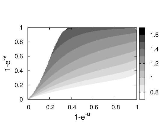
Figure 1: The contour lines of the function $c(u,v)$ in (19) predicted by the AdS/CFT correspondence are plotted against $\bar{u}=1-e^{-u}$ and $\bar{v}=1-e^{-v}$. The range of the function is $0.80\lesssim c(u,v)\lesssim 1.66$. The blank regions near $(\bar{u},\bar{v})=(1,0),(0,1),(1,1)$ represent the region of $(u,v)$ that cannot be realized according to the definition (10). See footnote 6.

In this paper we focus on the CPOs with the lowest dimension $\Delta=2$ given by

$${\cal O}_{ab}(x)=\mbox{tr}\Bigl{(}\phi_{a}(x)\phi_{b}(x)\Bigr{)}\;\;\mbox{with}\;\;a\neq b\ .$$ (11)

According to the above general argument, the correlation functions of the CPOs (11) can be parametrized as

$$\Bigl{\langle}{\cal O}_{45}(x_{1}){\cal O}_{54}(x_{2})\Bigr{\rangle} =\frac{\lambda^{2}}{(4\pi^{2})^{2}}\frac{c^{(2)}(\lambda,N)}{(x_{12})^{4}}\ ,$$ (12)

$$\Bigl{\langle}{\cal O}_{45}(x_{1}){\cal O}_{56}(x_{2}){\cal O}_{64}(x_{3})\Bigr{\rangle} =\frac{\lambda^{3}}{(4\pi^{2})^{3}N}\frac{c^{(3)}(\lambda,N)}{(x_{12})^{2}(x_{23})^{2}(x_{31})^{2}}\ ,$$ (13)

$$\Bigl{\langle}{\cal O}_{45}(x_{1}){\cal O}_{56}(x_{2}){\cal O}_{67}(x_{3}){\cal O}_{74}(x_{4})\Bigr{\rangle} =\frac{\lambda^{4}}{(4\pi^{2})^{4}N^{2}}\frac{c^{(4)}(\lambda,N;u,v)}{(x_{12})^{2}(x_{23})^{2}(x_{34})^{2}(x_{41})^{2}}\ .$$ (14)

These correlation functions have only connected contribution. By using the propagators for the scalar fields

$$\Bigl{\langle}\phi_{a}(x)_{pq}\phi_{b}(y)_{rs}\Bigr{\rangle}=\frac{g_{\rm YM}^{2}\delta_{ab}\delta_{ps}\delta_{qr}}{4\pi^{2}|x-y|^{2}}\ ,$$ (15)

where $p,q,r,s=1,\cdots,N$, one finds that the coefficients are given for the free theory by

$$\lim_{\lambda\rightarrow 0}c^{(2)}(\lambda,N)=\lim_{\lambda\rightarrow 0}c^{(3)}(\lambda,N)=\lim_{\lambda\rightarrow 0}c^{(4)}(\lambda,N;u,v)=1\ .$$ (16)

On the other hand, the AdS/CFT correspondence predicts that

$$\lim_{N\rightarrow\infty,\lambda\rightarrow\infty}c^{(2)}(\lambda,N)=\zeta\ ,$$ (17)

$$\lim_{N\rightarrow\infty,\lambda\rightarrow\infty}c^{(3)}(\lambda,N)=\zeta^{3/2}\ ,$$ (18)

$$\lim_{N\rightarrow\infty,\lambda\rightarrow\infty}c^{(4)}(\lambda,N;u,v)=\zeta^{2}c(u,v)\ .$$ (19)

Here $\zeta$ is a parameter associated with the normalization of the operator, which cannot be fixed by the AdS/CFT correspondence, while the non-renormalization property (7) implies $\zeta=1$. The prediction for $c(u,v)$ in (19) is obtained in ref. [95], and it is shown in figure 1. One finds that the function $c(u,v)$ has nontrivial dependence on $u$ and $v$, and in particular, it differs from 1, which implies that the four-point function is renormalized. This is consistent with the fact that the four-point function considered here is neither extremal nor next-to-extremal. The explicit form of $c(u,v)$ and useful expressions for its evaluation are given in appendix A.

3 ${\cal N}=4$ SYM on $R\times S^{3}$ and its large-$N$ reduction

In this section we review a non-perturbative formulation of planar ${\cal N}=4$ SYM on $R\times S^{3}$ proposed in ref. [44]. (See ref. [73] for a review.) This formulation is based on an extension of the large-$N$ reduction [50] to a curved manifold $S^{3}$. In section 3.1 we review the conformal map between ${\cal N}=4$ SYM on $R^{4}$ and that on $R\times S^{3}$. In section 3.2 we show how the PWMM is obtained from ${\cal N}=4$ SYM on $R\times S^{3}$ through a dimensional reduction. In section 3.3 we discuss how ${\cal N}=4$ SYM on $R\times S^{3}$ is retrieved from the PWMM through the novel large-$N$ reduction.

3.1 Conformal map between ${\cal N}=4$ SYM on $R^{4}$ and that on $R\times S^{3}$

It is well known that ${\cal N}=4$ SYM on $R^{4}$ has a moduli space, which is characterized by the vacuum expectation values of the scalar fields. The conformal symmetry is spontaneously broken except at the conformal point, which corresponds to a point in the moduli space where the vacuum expectation values all vanish. In section 2 we implicitly assumed that the theory is defined at the conformal point. In fact ${\cal N}=4$ SYM on $R^{4}$ at the conformal point is equivalent to ${\cal N}=4$ SYM on $R\times S^{3}$ through the conformal map. To see that, we apply a Weyl transformation defined by

$$A_{\mu}\mapsto A_{\mu}\ ,\quad\phi_{a}\mapsto e^{-\frac{\rho(x)}{2}}\phi_{a}\ ,\quad\delta_{\mu\nu}\mapsto g_{\mu\nu}=e^{\rho(x)}\delta_{\mu\nu}$$ (20)

to the action (1) of ${\cal N}=4$ SYM on $R^{4}$. This gives rise to ${\cal N}=4$ SYM on a curved space endowed with a metric $g_{\mu\nu}$ with the action

$$S=\frac{1}{g_{\rm YM}^{2}}\int d^{4}x\sqrt{g}\,\mbox{tr}\left(\frac{1}{4}g^{\mu\lambda}g^{\nu\rho}F_{\mu\nu}F_{\lambda\rho}+\frac{1}{2}g^{\mu\nu}D_{\mu}\phi_{a}D_{\nu}\phi_{a}+\frac{1}{12}{\cal R}\phi_{a}^{2}-\frac{1}{4}[\phi_{a},\phi_{b}]^{2}\right)\ ,$$ (21)

where ${\cal R}$ is the Ricci scalar constructed from $g_{\mu\nu}$.

Rewriting the metric on $R^{4}$ in the polar coordinates as

$$ds_{R^{4}}^{2}=dx^{\mu}dx^{\mu}=dr^{2}+r^{2}d\Omega_{3}^{2}=e^{\mu t}\left(dt^{2}+\left(\frac{2}{\mu}\right)^{2}d\Omega_{3}^{2}\right)=e^{\mu t}ds^{2}_{R\times S^{3}}\ ,$$ (22)

where $r=\frac{2}{\mu}e^{\frac{\mu}{2}t}$, one finds that $R^{4}$ is transformed to $R\times S^{3}$ by a Weyl transformation with $\rho(x)$ in (20) given by $\rho=-\mu t$. The radius of the resulting $S^{3}$ is given by

$$R_{S^{3}}=\frac{2}{\mu}\ .$$ (23)

Thus we have seen that ${\cal N}=4$ SYM on $R^{4}$ at the conformal point is equivalent to ${\cal N}=4$ SYM on $R\times S^{3}$.

The relation between the Cartesian coordinates and the polar coordinates of $R^{4}$ in (22) is given, for instance, as

$$x^{1} =r\,\cos\frac{\theta}{2}\,\cos\frac{\varphi+\psi}{2}\ ,\quad x^{2}=r\,\cos\frac{\theta}{2}\,\sin\frac{\varphi+\psi}{2}\ ,$$

$$x^{3} =r\,\sin\frac{\theta}{2}\,\cos\frac{-\varphi+\psi}{2}\ ,\quad x^{4}=r\,\sin\frac{\theta}{2}\,\sin\frac{-\varphi+\psi}{2}\ ,$$ (24)

where $0\leq\theta\leq\pi$, $0\leq\varphi<2\pi$ and $0\leq\psi<4\pi$, which we use later.

3.2 PWMM from ${\cal N}=4$ SYM on $R\times S^{3}$

Let us write down the action (21) explicitly in the case of $R\times S^{3}$. For that purpose we recall that $S^{3}$ can be viewed as the ${\rm SU}(2)$ group manifold. The isometry of $S^{3}$ corresponds to the left and right translations on the ${\rm SU}(2)$ group manifold as one can see from the relation ${\rm SO}(4)={\rm SU}(2)\times{\rm SU}(2)$. As is well known, one can construct the right-invariant 1-forms $e^{i}_{\bar{\mu}}$, where $i=1,2,3$ and $\bar{\mu}$ stands for $\theta,\phi,\psi$. (Note that $\mu$ in (21) represents either $t$ or $\bar{\mu}$.) The 1-forms $e^{i}_{\bar{\mu}}$ are called “dreibein” and satisfy the Maurer-Cartan equation

$$\partial_{\bar{\mu}}\,e^{i}_{\bar{\nu}}-\partial_{\bar{\nu}}\,e^{i}_{\bar{\mu}}-\mu\,\epsilon_{ijk}\,e^{j}_{\bar{\mu}}\,e^{k}_{\bar{\nu}}=0\ .$$ (25)

By using the inverse of $e^{i}_{\bar{\mu}}$ denoted by $e_{i}^{\bar{\mu}}$, one can also construct the Killing vector

$${\cal L}_{i}=-\frac{i}{\mu}\,e^{\bar{\mu}}_{i}\,\partial_{\bar{\mu}}\ ,$$ (26)

which represents the generators of the left translation and satisfies the ${\rm SU}(2)$ algebra $[{\cal L}_{i},{\cal L}_{j}]=i\epsilon_{ijk}{\cal L}_{k}$. The ${\rm SO}(4)$-isometric metric on $S^{3}$ is given in terms of $e^{i}_{\bar{\mu}}$ as

$$g_{\bar{\mu}\bar{\nu}}=e^{i}_{\bar{\mu}}\,e^{i}_{\bar{\nu}}\ ,$$ (27)

and the Ricci scalar constructed from $g_{\bar{\mu}\bar{\nu}}$ takes a constant value $\frac{3}{2}\,\mu^{2}$.

We expand the gauge field on $S^{3}$ with respect to $e^{i}_{\bar{\mu}}$ as $A_{\bar{\mu}}=e^{i}_{\bar{\mu}}X_{i}$, and denote $\phi_{a}$ as $X_{a}$. Then, using (25), (26) and (27), we can rewrite (21) in terms of $X_{i}$ and $X_{a}$ as

$$S =\frac{V_{S^{3}}}{g_{\rm YM}^{2}}\int dt\,\frac{d\Omega_{3}}{2\pi^{2}}\,\mbox{tr}\left[\frac{1}{2}\,(D_{t}X_{i}-i\mu{\cal L}_{i}A_{t})^{2}+\frac{1}{2}\,\left\{\mu X_{i}+i\epsilon_{ijk}\left(\mu{\cal L}_{j}X_{k}+\frac{1}{2}[X_{j},X_{k}]\right)\right\}^{2}\right.$$

$$\qquad\qquad\qquad\qquad\;\;\;\left.+\frac{1}{2}\,(D_{t}X_{i})^{2}-\frac{1}{2}\,(\mu{\cal L}_{i}X_{a}+[X_{i},X_{a}])^{2}+\frac{1}{8}\,\mu^{2}X_{a}^{2}-\frac{1}{4}\,[X_{a},X_{b}]^{2}\right]\ ,$$ (28)

where $d\Omega_{3}=\frac{1}{8}\sin\theta\,d\theta\,d\phi\,d\psi$ is the volume element of a unit $S^{3}$ and the covariant derivative is defined by $D_{t}=\partial_{t}+i\,[A_{t},\ \cdot\ ]$.

Let us perform a dimensional reduction over $S^{3}$ [60, 96] by making the fields depend only on $t$, namely by setting ${\cal L}_{i}A_{t}=0$, ${\cal L}_{i}X_{i}=0$ and ${\cal L}_{i}X_{a}=0$. The resulting theory is nothing but the PWMM, and its complete form including the fermion fields is

$$S_{\rm PW}=\frac{1}{g_{\rm PW}^{2}}\int dt\,\mbox{tr} \left(\frac{1}{2}\,(D_{t}X_{M})^{2}-\frac{1}{4}\,[X_{M},X_{N}]^{2}+\frac{1}{2}\,\mu^{2}X_{i}^{2}+\frac{1}{8}\,\mu^{2}X_{a}^{2}+i\,\mu\,\epsilon_{ijk}\,X_{i}X_{j}X_{k}\right.$$

$$\left.+\frac{1}{2}\,\Psi^{\dagger}D_{t}\Psi-\frac{1}{2}\,\Psi^{\dagger}\gamma_{M}[X_{M},\Psi]+\frac{3}{8}\,i\,\mu\,\Psi^{\dagger}\gamma_{123}\Psi\right)\ ,$$ (29)

where $M$ runs from 1 to 9. This is a consistent truncation in the sense that every classical solution in (29) is a classical solution in (28). The PWMM has the ${\rm SU}(2|4)$ symmetry with 16 supercharges, which is a subgroup of ${\rm PSU}(2,2|4)$ of ${\cal N}=4$ SYM. By setting $\mu=0$ in eq. (29), one obtains the Matrix Theory [97]. In fact the PWMM can be viewed as a mass deformation of the Matrix Theory preserving its SUSYs completely.

The PWMM has many discrete vacua given by

$$X_{i}=\mu L_{i}=\mu\bigoplus_{I=1}^{\nu}\Bigl{(}L_{i}^{(n_{I})}\otimes{\bf 1}_{k_{I}}\Bigr{)}\ ,\quad\quad X_{a}=0\ ,$$ (30)

where $L_{i}^{(r)}$ are the $r$-dimensional irreducible representation of the SU$(2)$ generators obeying

$$[L_{i}^{(n)},L_{j}^{(n)}]=i\,\epsilon_{ijk}\,L_{k}^{(n)}\ .$$ (31)

The parameters $n_{I}$ and $k_{I}$ in (30) have to satisfy the relation

$$\sum_{I=1}^{\nu}n_{I}k_{I}=N\ .$$ (32)

These vacua preserve the SU$(2|4)$ symmetry, and they are all degenerate. Since the generators $L_{i}^{(n)}$ satisfy $\sum_{i=1}^{3}(L_{i}^{(n)})^{2}=\frac{1}{4}(n^{2}-1)\,{\bf 1}_{n}$, they represent a fuzzy sphere [58]. The classical vacua (30) therefore represent multi-fuzzy-sphere configurations with different radii $\frac{\mu}{2}\sqrt{(n_{I})^{2}-1}$ and multiplicity $k_{I}$.

3.3 ${\cal N}=4$ SYM on $R\times S^{3}$ from PWMM

In order to retrieve ${\cal N}=4$ SYM on $R\times S^{3}$ from its reduced model (29) in the planar limit, we need to pick up a particular background from (30) and consider the theory (29) around it [44]. Let us consider the background (30) with

$$k_{I}=k\ ,\quad n_{I}=n+I-\frac{\nu+1}{2}\quad\quad\mbox{for $I=1,\cdots,\nu$}$$ (33)

and take the large-$N$ limit in such a way that

$$k\rightarrow\infty,\;\;\frac{n}{\nu}\rightarrow\infty,\;\;\nu\rightarrow\infty,\;\;\mbox{with}\;\;\tilde{\lambda}\equiv\frac{g_{\rm PW}^{2}k}{n}\;\;\mbox{fixed}\ .$$ (34)

Note that the $k\rightarrow\infty$ limit ensures the dominance of planar diagrams in the reduced model. Then the resulting theory is equivalent to the planar limit of ${\cal N}=4$ SYM on $R\times S^{3}$ with the radius (23) of $S^{3}$ and the ’t Hooft coupling constant given by

$$\lambda=\tilde{\lambda}\,V_{S^{3}}\ ,$$ (35)

where $V_{S^{3}}=2\pi^{2}(R_{S^{3}})^{3}=16\pi^{2}/\mu^{3}$ is the volume of $S^{3}$.

This equivalence may be viewed as an extension of the large-$N$ reduction to a curved space $S^{3}$. The original idea [50] for theories compactified on a torus can fail due to the instability of the ${\rm U}(1)^{D}$ symmetric vacuum of the reduced model [52]. This problem is avoided in the above new proposal since the PWMM is a massive theory and the vacuum preserves the maximal SUSY. The instanton transition to other vacua is suppressed due to the $k\rightarrow\infty$ limit. Note also that the “fuzziness” of the spheres disappears in the $k\rightarrow\infty$ limit since the UV/IR mixing effects come only from non-planar diagrams. The SU($N$) gauge symmetry of the PWMM (with the gauge function depending only on $t$) is translated into the four-dimensional SU($k$) gauge symmetry of ${\cal N}=4$ SYM. Viewed as a regularization of ${\cal N}=4$ SYM on $R\times S^{3}$, the present formulation respects the ${\rm SU}(2|4)$ symmetry with 16 supercharges of the PWMM, and in the limit (34) the symmetry is expected to enhance to the full superconformal symmetry ${\rm PSU}(2,2|4)$ with 32 supercharges of ${\cal N}=4$ SYM. Since any kind of UV regularization breaks the conformal symmetry, this regularization should be considered optimal from the viewpoint of preserving SUSY.

4 Correlation functions of CPOs from PWMM

In this section we show how one can obtain the correlation functions of CPOs in ${\cal N}=4$ SYM by calculating their counterparts in the PWMM. In particular, we perform explicit calculations in the free theory case and confirm that the results obtained in the limit (34) from the PWMM around the background (33) reproduce the correlation functions of CPOs in ${\cal N}=4$ SYM.

4.1 Correlation functions of CPOs in ${\cal N}=4$ SYM on $R\times S^{3}$

Let us first define correlation functions of CPOs in ${\cal N}=4$ SYM on $R\times S^{3}$. We find from (20) that the six scalar fields on $R^{4}$ are related to those on $R\times S^{3}$ as

$$\phi_{a}(x)=e^{-\frac{\mu}{2}t}\phi_{a}(t,\Omega_{3})\ .$$ (36)

Correspondingly, the free propagator (15) on $R^{4}$ is translated to that on $R\times S^{3}$ as

$$\Bigl{\langle}\phi_{a}(t,\Omega_{3})_{pq}\,\phi_{b}(t^{\prime},\Omega_{3}^{\prime})_{rs}\Bigr{\rangle}=\frac{g_{\rm YM}^{2}\delta_{ab}\delta_{ps}\delta_{qr}e^{\frac{\mu}{2}(t+t^{\prime})}}{4\pi^{2}|x-x^{\prime}|^{2}}\ .$$ (37)

As in (2), CPOs in ${\cal N}=4$ SYM on $R\times S^{3}$ are defined by

$${\cal O}_{I}(t,\Omega_{3})=T_{I}^{a_{1}a_{2}\cdots a_{\Delta_{I}}}\mbox{tr}\Bigl{(}\phi_{a_{1}}(t,\Omega_{3})\phi_{a_{2}}(t,\Omega_{3})\cdots\phi_{a_{\Delta_{I}}}(t,\Omega_{3})\Bigr{)}\ .$$ (38)

In particular, the CPOs on $R\times S^{3}$ with the lowest energy corresponding to (11) are

$${\cal O}_{ab}(t,\Omega_{3})=\mbox{tr}\Bigl{(}\phi_{a}(t,\Omega_{3})\phi_{b}(t,\Omega_{3})\Bigr{)}\;\;\;\mbox{with}\;\;a\neq b\ .$$ (39)

By using (37), one obtains, for instance, the two-point function of ${\cal O}_{ab}(t,\Omega_{3})$ in the free theory as

$$\Bigl{\langle}{\cal O}_{ab}(t,\Omega_{3})\,{\cal O}_{ab}(t^{\prime},\Omega_{3}^{\prime})\Bigr{\rangle}_{\rm free}=\frac{\lambda^{2}e^{\mu(t+t^{\prime})}}{16\pi^{4}|x-x^{\prime}|^{4}}\ .$$ (40)

In order to relate these operators to their counterparts in the PWMM, we need to integrate ${\cal O}_{I}(t,\Omega_{3})$ over a unit $S^{3}$ and define an operator

$$\bar{{\cal O}}_{I}(t)\equiv\int\frac{d\Omega_{3}}{2\pi^{2}}\,{\cal O}_{I}(t,\Omega_{3})\ ,\quad$$ (41)

and, in particular,

$$\bar{{\cal O}}_{ab}(t)\equiv\int\frac{d\Omega_{3}}{2\pi^{2}}\,{\cal O}_{ab}(t,\Omega_{3})\ .$$ (42)

The two-point function of $\bar{{\cal O}}_{ab}(t)$ can be calculated in the free theory by using (24) and (40) as

$$\Bigl{\langle}\bar{{\cal O}}_{ab}(t)\bar{{\cal O}}_{ab}(t^{\prime})\Bigr{\rangle}_{\rm free} =\frac{\lambda^{2}}{16\pi^{4}}e^{\mu(t+t^{\prime})}\int\frac{d\Omega_{3}}{2\pi^{2}}\frac{1}{|x-x^{\prime}|^{4}}$$

$$=\frac{\lambda^{2}}{16^{2}\pi^{6}}e^{\mu(t+t^{\prime})}\int_{0}^{\pi}\!\!\!d\theta\int_{0}^{2\pi}\!\!\!d\varphi\int_{0}^{4\pi}\!\!\!d\psi\sin\theta\frac{1}{(r^{2}+r^{\prime}{}^{2}-2rr^{\prime}\cos\frac{\theta}{2}\cos\frac{\varphi+\psi}{2})^{2}}$$

$$=\frac{\lambda^{2}\mu^{4}}{(16\pi^{2})^{2}}\frac{e^{-\mu|t-t^{\prime}|}}{1-e^{-\mu|t-t^{\prime}|}}\ ,$$ (43)

where we have fixed $x^{\prime}$ to $(r^{\prime},0,0,0)$ without loss of generality.

In a similar manner, the three-point and four-point functions are calculated in the free theory as

$$N\Bigl{\langle}\bar{{\cal O}}_{45}(t_{1})\bar{{\cal O}}_{56}(t_{2})\bar{{\cal O}}_{64}(t_{3})\Bigr{\rangle}_{\rm free}=-\frac{\lambda^{3}\mu^{6}}{(16\pi^{2})^{3}}\log(1-e^{-\frac{\mu}{2}(|t_{1}-t_{2}|+|t_{2}-t_{3}|+|t_{3}-t_{1}|)})\ ,$$

$$N^{2}\Bigl{\langle}\bar{{\cal O}}_{45}(t_{1})\bar{{\cal O}}_{56}(t_{2})\bar{{\cal O}}_{67}(t_{3})\bar{{\cal O}}_{74}(t_{4})\Bigr{\rangle}_{\rm free}=\frac{\lambda^{4}\mu^{8}}{(16\pi^{2})^{4}}\mbox{Li}_{2}(e^{-\frac{\mu}{2}(|t_{1}-t_{2}|+|t_{2}-t_{3}|+|t_{3}-t_{4}|+|t_{4}-t_{1}|)})\ ,$$ (44)

where $\mbox{Li}_{2}$ is the dilogarithmic function defined by $\mbox{Li}_{2}(z)=-\int_{0}^{z}\frac{\log(1-u)}{u}du$. In fact the correlation functions in (43) and (44) have only planar contribution in the free theory.

4.2 Corresponding correlation functions in PWMM

As we reviewed in section 3.3, ${\cal N}=4$ SYM on $R\times S^{3}$ is equivalent to the PWMM in the large-$N$ limit. In this equivalence, the operators in the PWMM corresponding to (41) in ${\cal N}=4$ SYM are

$${\cal O}_{I}(t)=T_{I}^{a_{1}a_{2}\cdots a_{\Delta_{I}}}\mbox{tr}\left(X_{a_{1}}(t)X_{a_{2}}(t)\cdots X_{a_{\Delta_{I}}}(t)\right)\ .$$ (45)

The relationship between the correlation functions is given by

$$N^{M-2}\Bigl{\langle}\bar{{\cal O}}_{I_{1}}(t_{1})\cdots\bar{{\cal O}}_{I_{M}}(t_{M})\Bigr{\rangle}=\frac{k^{M-2}}{n^{M}\nu}\Bigl{\langle}{\cal O}_{I_{1}}(t_{1})\cdots{\cal O}_{I_{M}}(t_{M})\Bigr{\rangle}_{\rm PW}\ ,$$ (46)

where the symbol $\langle\ \cdot\ \rangle_{\rm PW}$ on the right-hand side represents a VEV with respect to the PWMM (29) around the background (33), and it is assumed that the limit (34) is taken. The trace over $N\times N$ matrices in (45), which ensures the gauge invariance, actually corresponds to integrating over $S^{3}$ and taking the trace over $k\times k$ indices. Both sides of (46) represent planar and connected contribution, and the factors $N^{M-2}$, $k^{M-2}$ on each side make the quantities finite in the planar limit. This kind of correspondence holds for general gauge-invariant operators in ${\cal N}=4$ SYM on $R\times S^{3}$.

Here we show explicitly in the free theory that (46) holds for correlation functions defined by (43) and (44). Note that the corresponding correlation functions in the PWMM have only planar contribution in the free theory similarly to the situation in ${\cal N}=4$ SYM. In order to calculate the right-hand side of (46) around the background (33) in the PWMM, we expand the $(I,J)$ block of $X_{a}$ —denoted by $X^{(I,J)}_{a}$— in terms of the fuzzy spherical harmonics defined in (82) as

$$X^{(I,J)}_{a}(t)=\sum_{j=\frac{1}{2}|n_{I}-n_{J}|}^{\frac{1}{2}(n_{I}+n_{J})-1}\sum_{m=-j}^{j}x^{(I,J)}_{ajm}(t)\otimes Y_{jm}^{(n_{I},n_{J})}\ .$$ (47)

Note that $X^{(I,J)}_{a}(t)$ is a $(n_{I}k)\times(n_{J}k)$ matrix, while $x^{(I,J)}_{ajm}(t)$ is a $k\times k$ matrix. Using (83), we find that the operator corresponding to (42) can be expressed as

$${\cal O}_{ab}(t)\equiv\mbox{tr}(X_{a}(t)X_{b}(t))=\sum_{I,J}\sum_{j,m}(-1)^{m-\frac{1}{2}(n_{I}-n_{J})}\mbox{tr}\Bigl{(}x_{ajm}^{(n_{I},n_{J})}x_{bj-m}^{(n_{J},n_{I})}\Bigr{)}\ .$$ (48)

Expanding the action (29) around the background (33), we find that the quadratic terms in $X_{a}$ is diagonalized in terms of $x_{ajm}(t)$ as

$$\frac{1}{2g_{\rm PW}^{2}}\int dt\,\mbox{tr}\left(-X_{a}\partial_{t}^{2}X_{a}+\mu^{2}X_{a}[L_{i},[L_{i},X_{a}]]+\frac{\mu^{2}}{4}X_{a}^{2}\right)$$

$$=\frac{1}{2g_{\rm PW}^{2}}\int dt\sum_{I,J}\sum_{j,m}(-1)^{m-\frac{1}{2}(n_{I}-n_{J})}\mbox{tr}\left(x^{(I,J)}_{ajm}\left(-\partial_{t}^{2}+\mu^{2}\left(j+\frac{1}{2}\right)^{2}\right)x^{(J,I)}_{aj\>-m}\right),$$ (49)

where $L_{i}$ is given by (30). From (49), we can read off the free propagator for $x^{(I,J)}_{ajm}$ as

$$\Bigl{\langle}\Bigl{(}x^{(I,J)}_{ajm}(t)\Bigr{)}_{pq}\Bigl{(}x^{(I^{\prime},J^{\prime})}_{a^{\prime}j^{\prime}m^{\prime}}(t^{\prime})\Bigr{)}_{rs}\Bigr{\rangle} =\frac{g_{\rm PW}^{2}(-1)^{m-\frac{1}{2}(n_{I}-n_{J})}}{2\mu(j+\frac{1}{2})}e^{-\mu(j+\frac{1}{2})|t-t^{\prime}|}$$

$$\quad\times\delta_{aa^{\prime}}\delta_{IJ^{\prime}}\delta_{JI^{\prime}}\delta_{jj^{\prime}}\delta_{m\>-m^{\prime}}\delta_{ps}\delta_{qr}\ ,$$ (50)

where $0\leq p,q,r,s\leq k$.

Let us calculate the two-point function corresponding to (43) in the free theory. By using (50), we obtain

$$\frac{1}{n^{2}\nu}\Bigl{\langle}{\cal O}_{ab}(t){\cal O}_{ab}(t^{\prime})\Bigr{\rangle}_{\rm PW,free}=\frac{g_{\rm PW}^{4}k^{2}}{2\mu^{2}n^{2}\nu}\sum_{I,J=1}^{\nu}\sum_{j=\frac{1}{2}|n_{I}-n_{J}|}^{\frac{1}{2}(n_{I}+n_{J})-1}\frac{e^{-\mu(2j+1)|t-t^{\prime}|}}{j+\frac{1}{2}}\ .$$ (51)

We can show that (51) agrees with (43) in the limit (34). For simplicity, we first take the $n\rightarrow\infty$ limit. Then, (51) can be evaluated as

$$\frac{g_{\rm PW}^{4}k^{2}}{\mu^{2}n^{2}\nu}\int_{\mu|t-t^{\prime}|}^{\infty}ds\sum_{I,J=1}^{\nu}\sum_{j=\frac{1}{2}|I-J|}^{\infty}e^{-(2j+1)s} =\frac{g_{\rm PW}^{4}k^{2}}{\mu^{2}n^{2}\nu}\int_{\mu|t-t^{\prime}|}^{\infty}ds\frac{e^{-s}}{1-e^{-2s}}\sum_{I,J=1}^{\nu}e^{-|I-J|s}$$

$$=\frac{g_{\rm PW}^{4}k^{2}}{\mu^{2}n^{2}}\int_{\mu|t-t^{\prime}|}^{\infty}ds\frac{e^{-s}}{(1-e^{-s})^{2}}$$

$$=\frac{g_{\rm PW}^{4}k^{2}}{\mu^{2}n^{2}}\frac{e^{-\mu|t-t^{\prime}|}}{1-e^{-\mu|t-t^{\prime}|}}\ .$$ (52)

By using (35), we find that the last expression indeed agrees with (43).

Similarly, one can calculate the three-point and four-point functions corresponding to those in (44) in the free theory. The results are

$$\frac{k}{n^{3}\nu}\Bigl{\langle}{\cal O}_{45}(t_{1}){\cal O}_{56}(t_{2}){\cal O}_{64}(t_{3})\Bigr{\rangle}_{\rm PW,free}\!=\!\frac{g_{\rm PW}^{6}k^{3}}{4\mu^{3}n^{3}\nu}\!\sum_{I,J=1}^{\nu}\!\sum_{j=\frac{1}{2}|n_{I}-n_{J}|}^{\frac{1}{2}(n_{I}+n_{J})-1}\!\!\!\frac{e^{-\mu(j+\frac{1}{2})(|t_{1}-t_{2}|+|t_{2}-t_{3}|+|t_{3}-t_{1}|)}}{(j+\frac{1}{2})^{2}}\ ,$$

$$\frac{k^{2}}{n^{4}\nu}\Bigl{\langle}{\cal O}_{45}(t_{1}){\cal O}_{56}(t_{2}){\cal O}_{67}(t_{3}){\cal O}_{74}(t_{4})\Bigr{\rangle}_{\rm PW,free}$$

$$=\frac{g_{\rm PW}^{8}k^{4}}{8\mu^{4}n^{4}\nu}\sum_{I,J=1}^{\nu}\sum_{j=\frac{1}{2}|n_{I}-n_{J}|}^{\frac{1}{2}(n_{I}+n_{J})-1}\frac{e^{-\mu(j+\frac{1}{2})(|t_{1}-t_{2}|+|t_{2}-t_{3}|+|t_{3}-t_{4}|+|t_{4}-t_{1}|)}}{(j+\frac{1}{2})^{3}}\ .$$ (53)

Similarly to (52), one can show that the three-point and four-point functions in (53) agree with those in (44) in the limit (34). Thus we have confirmed that (46) holds in the free theory case.

Figure 2: The four-point function (53) for the PWMM in the free theory case with $\mu=2$ is plotted for backgrounds (33) with $(n,\nu)=(1,1)$, $(\frac{3}{2},2)$, $(3,3)$, $(\frac{11}{2},4)$. The normalization constant in (44) is chosen such that it formally corresponds to $\lambda=16$. We observe clear convergence towards the result (44) for ${\cal N}=4$ SYM in the free theory case represented by the solid line.

Let us discuss the rate of convergence. As an example, we consider the four-point function in the PWMM given by (53), and see how it converges to that in ${\cal N}=4$ SYM given by (44) in the free theory case. Here we take the limit (34) with a choice $n=\frac{1}{2}\nu^{2}-\nu+\frac{3}{2}$, which amounts to considering a sequence

$$(n,\nu)=(1,1),\ \left(\frac{3}{2},2\right),\ (3,3),\ \left(\frac{11}{2},4\right),\cdots\ .$$ (54)

In figure 2 we plot the results for this sequence, which show clear convergence towards the result for ${\cal N}=4$ SYM. In our Monte Carlo simulation, which will be discussed in the next section, we take the background $(n,\nu)=(\frac{3}{2},2)$ in this sequence.

5 Monte Carlo method

In this section we discuss our Monte Carlo method for studying ${\cal N}=4$ SYM. Due to the large-$N$ reduction, ${\cal N}=4$ SYM on $R\times S^{3}$ is equivalent to the PWMM (29), which we actually simulate. Since the PWMM is a one-dimensional theory, we need to introduce an IR and UV cutoffs in the $t$-direction. The IR cutoff is introduced by compactifying the $t$-direction to a circle of circumference $\beta$ with periodic boundary conditions on both scalars $X_{i}(t)$ and fermions $\Psi_{\alpha}(t)$. Following refs. [11, 13, 14, 16, 18], we introduce a sharp UV cutoff in the Fourier space after fixing the gauge completely. This is possible since the $t$-direction is one-dimensional.

First we take the static diagonal gauge

$$A(t)=\frac{1}{\beta}\,{\rm diag}(\alpha_{1},\cdots,\alpha_{N})\ ,$$ (55)

where $\alpha_{a}$ are constant in time. This condition does not fix the gauge completely, and in fact there is a residual gauge symmetry

$$\alpha_{a}\mapsto\alpha_{a}+2\pi\nu_{a}\ ,\quad\tilde{X}_{i,n}^{ab}\mapsto\tilde{X}_{i,n-\nu_{a}+\nu_{b}}^{ab}\ ,\quad\tilde{\Psi}_{\alpha,n}^{ab}\mapsto\tilde{\Psi}_{\alpha,n-\nu_{a}+\nu_{b}}^{ab}\ ,$$ (56)

where $\nu_{a}$ is an integer. This residual symmetry can be fixed by imposing $-\pi<\alpha_{a}\leq\pi$. Corresponding to the above gauge choice, the Faddeev-Popov term

$$S_{\rm FP}=-\sum_{a<b}2\ln{\left|\sin{\frac{\alpha_{a}-\alpha_{b}}{2}}\right|}$$ (57)

should be added in the action. Then we introduce a cutoff $\Lambda$ in the Fourier-mode expansion

$$X_{i}(t)=\sum_{n=-\Lambda}^{\Lambda}\tilde{X}_{i,n}e^{i\omega nt}\ ,\quad\omega\equiv\frac{2\pi}{\beta}\ ,$$ (58)

and similarly for the fermions [9]. Since there are no UV divergences in the one-dimensional theory, one can obtain the original PWMM by taking the limits $\beta\rightarrow\infty\ ,\frac{\Lambda}{\beta}\rightarrow\infty$.

The integration over fermionic variables yields a Pfaffian, which is complex in general. As is done in the previous works [11, 13, 14, 16, 18] on the D0-brane system, we simply take the absolute value of the Pfaffian assuming that the phase does not affect the results. The model obtained in this way can be simulated by the Rational Hybrid Monte Carlo (RHMC) algorithm [99]. This method has been applied extensively to the D0-brane system corresponding to $\mu=0$, and the results confirmed the gauge/gravity duality for various observables [11, 13, 14, 16, 18]. See appendix B of ref. [18] for the details of the algorithm.

We start our simulation with an initial configuration given by (33) with the parameters $(n,\nu,k)=(\frac{3}{2},2,2)$, which corresponds to the matrix size $N=6$. Since the parameter $\mu$ in the action (29) can be scaled away by appropriate redefinition of the fields and the parameters, we take $\mu=2$ without loss of generality, which corresponds to a unit sphere $S^{3}$ due to (23). Then, for the chosen background $(n,\nu,k)=(\frac{3}{2},2,2)$, the relation between $g_{\rm PW}^{2}N$ and $\lambda$ becomes

$$\lambda=\frac{4}{9}\pi^{2}(g_{\rm PW}^{2}N)\ ,$$ (60)

due to (34) and (35). We choose the coupling constant of the PWMM as $g_{\rm PW}^{2}N=0.125$, $1.0$, $3.64$, which correspond to the coupling constant of $\mathcal{N}=4$ SYM given by $\lambda=0.55$, $4.39$, $16.0$, respectively, according to (60). For these values of $\lambda$, we find that transitions to other vacua do not occur during the simulation as we discuss in appendix E. The IR cutoff in the $t$-direction is taken as $\beta=10.0$, $5.0$, $3.25$, respectively, for each couplings, while the UV cutoff parameter $\Lambda$ in the $t$-direction is taken as $\Lambda=12$ for all cases.

The dependence of our results on the regularization parameters is discussed in appendix F. In particular, we have checked that our results for the two-point functions after taking the ratio to the free theory case do not change significantly for larger $n$, $\nu$ and $k$. Also we find that finite-$\Lambda$ effects are negligible, and hence the SUSY breaking by such effects can be safely ignored.

6 Results

In this section we present our results for the correlation functions of CPOs in $\mathcal{N}=4$ SYM. These results are obtained by using the relationship (46) and calculating the corresponding correlation functions in the PWMM by the Monte Carlo method described in the previous section.

In figure 3 (Left) we present our results for the two-point function

$$G^{(2)}(p,-p) =\left(\frac{\mu}{g_{\rm PW}^{2}N}\right)^{2}\left\langle\widetilde{O}_{45}(p)\,\widetilde{O}_{54}(-p)\right\rangle_{\rm PW}\ ,$$ (61)

where we have defined the Fourier transform of an operator ${\cal O}(t)$ as

$$\widetilde{\cal O}(p)=\frac{1}{\beta}\int_{0}^{\beta}dt\,{\cal O}(t)\,e^{-ipt}\ .$$ (62)

In order to study the non-renormalization property, we compare our data with the free theory results, which are calculated analytically by just switching off the interaction terms in the reduced model with the same regularization parameters. (See appendix D for explicit results not only for two-point functions but also for three-point and four-point functions.) In figure 3 (Right) we plot the ratio

$$R^{\rm(2)}(p,-p)=\frac{\Big{\langle}\widetilde{O}_{45}(p)\,\widetilde{O}_{54}(-p)\Big{\rangle}_{\rm PW}}{\Big{\langle}\widetilde{O}_{45}(p)\,\widetilde{O}_{54}(-p)\Big{\rangle}_{\rm PW,free}}\ .$$ (63)

The momentum dependence of the correlation function is almost canceled by taking the ratio, and we observe a nice plateau behavior. By fitting $R^{\rm(2)}(p,-p)$ to a constant in the momentum region $p=\frac{2\pi n}{\beta}$, where $6\leq n\leq\Lambda\equiv 12$, we obtain $0.917(2)$, $0.805(2)$, $0.658(3)$ for $\lambda=0.55$, $4.39$, $16.0$, respectively. In figure 3 (Left) we also plot the free theory results multiplied by the overall constants obtained in this way. Thus we find that our data are in good agreement with the corresponding free theory result up to an overall constant depending on $\lambda$. This is remarkable considering that the value of the two-point function changes by orders of magnitude as a function of $p$.

Figure 3: (Left) The two-point function $G^{(2)}(p,-p)$ is plotted as a function of $p$ in the log scale for $\lambda=0.55$, $4.39$, $16.0$. The curves represent the corresponding free theory results multiplied by the values obtained as the height of the plateau in the right panel. (Right) The ratio $R^{\rm(2)}(p,-p)$ of the two-point function to the corresponding free theory result is plotted for $\lambda=0.55$, $4.39$, $16.0$. The horizontal lines represent the fits to the plateau behavior, which give estimates for $c^{(2)}$.

As we have reviewed in section 2, the form of the two-point function is fixed by the conformal invariance of $\mathcal{N}=4$ SYM, and therefore the ratio $R^{\rm(2)}(p,-p)$ should become a constant, which corresponds to $c^{(2)}$ in (12) in the large-$N$ limit (34). The height of the plateau in figure 3 (Right) gives an estimate for $c^{(2)}$ with the present matrix size, which decreases from 1 as $\lambda$ increases. On the other hand, the SUSY non-renormalization property (7) implies that $c^{(2)}=1$. We therefore consider that the height of the plateau approaches 1 for any $\lambda$ as we take the limit (34).

Figure 4: (Left) The three-point function $G^{(3)}(p,0,-p)$ is plotted as a function of $p$ in the log scale for $\lambda=0.55$, $4.39$, $16.0$. The curves represent the corresponding free theory results multiplied by $(c^{(2)})^{3/2}$ using $c^{(2)}$ obtained from figure 3 for each $\lambda$. (Right) The ratio $R^{\rm(3)}(p,0,-p)$ of the three-point function to the corresponding free theory result is plotted for $\lambda=0.55$, $4.39$, $16.0$. The horizontal line represents $(c^{(2)})^{3/2}$ using $c^{(2)}$ obtained from figure 3.

Let us move on to the three-point function

$$G^{(3)}(p,0,-p)=\left(\frac{\mu}{g_{\rm PW}^{2}N}\right)^{3}\Big{\langle}\tilde{{\cal O}}_{45}(p)\tilde{{\cal O}}_{56}(0)\tilde{{\cal O}}_{64}(-p)\Big{\rangle}_{\rm PW}\ ,$$ (64)

which is shown in figure 4 together with the ratio

$$R^{\rm(3)}(p,0,-p)=\frac{\Big{\langle}\tilde{{\cal O}}_{45}(p)\tilde{{\cal O}}_{56}(0)\tilde{{\cal O}}_{64}(-p)\Big{\rangle}_{\rm PW}}{\Big{\langle}\tilde{{\cal O}}_{45}(p)\tilde{{\cal O}}_{56}(0)\tilde{{\cal O}}_{64}(-p)\Big{\rangle}_{\rm PW,free}}\ .$$ (65)

We observe that the three-point function agrees with the free theory results up to an overall constant. Since the form of the three-point function is determined by the conformal symmetry as in the case of two-point functions, the ratio $R^{\rm(3)}(p,0,-p)$ should become a constant, which corresponds to $c^{(3)}$ in (13), in the limit (34). The height of the plateau in figure 4 (Right) gives an estimate for $c^{(3)}$ with the present matrix size.

The AdS/CFT correspondence predicts (17) and (18), which implies

$$c^{(3)}=(c^{(2)})^{3/2}\ .$$ (66)

In order to see whether our data is consistent with (66), we use the value of $c^{(2)}$ extracted from our results for two-point functions, and plot $(c^{(2)})^{3/2}$ in figure 4 (Right). The margin between the lines represents the fitting error in estimating $c^{(2)}$ from the plateau height. Our results for the ratio $R^{\rm(3)}(p,0,-p)$ are in reasonable agreement with $(c^{(2)})^{3/2}$ obtained from the two-point function, which implies consistency with (66). Thus we find that the weaker form of the SUSY non-renormalization property holds even at the regularized level. In the large-$N$ limit (34), both sides of (66) are expected to approach 1.

Figure 5: (Left) The four-point function $G^{(4)}(p_{1},p_{2},p_{3},p_{4})$ is plotted for three types of momentum configuration $(p_{1},p_{2},p_{3},p_{4})=(p,0,0,-p),~{}(p,-p,p,-p),~{}(p,p,-p,-p)$ as a function of $p$ in the log scale for $\lambda=16.0$. The curves represent the corresponding free theory results multiplied by $(c^{(2)})^{2}$ using $c^{(2)}$ obtained from figure 3. (Right) The ratio $R^{\rm(4)}(p_{1},p_{2},p_{3},p_{4})$ of the four-point function to the corresponding free theory result is plotted for three types of momentum configuration $(p_{1},p_{2},p_{3},p_{4})=(p,0,0,-p),~{}(p,-p,p,-p),~{}(p,p,-p,-p)$ as a function of $p$ for $\lambda=16.0$. The horizontal line represents $(c^{(2)})^{2}$ using $c^{(2)}$ obtained from figure 3.

Finally we discuss our results for the four-point functions

$$G^{(4)}(p_{1},p_{2},p_{3},p_{4})=\left(\frac{\mu}{g_{\rm PW}^{2}N}\right)^{4}\Big{\langle}\tilde{{\cal O}}_{45}(p_{1})\tilde{{\cal O}}_{56}(p_{2})\tilde{{\cal O}}_{67}(p_{3})\tilde{{\cal O}}_{74}(p_{4})\Big{\rangle}_{\rm PW}\ .$$ (67)

Since the four-point functions we study are neither extremal nor next-to-extremal, the SUSY non-renormalization property can be violated. Indeed the AdS/CFT correspondence predicts the explicit form of the violation given by (19). The prediction of the AdS/CFT correspondence is obtained in the strong coupling limit, and the violation is expected to become smaller as the coupling constant decreases. Therefore, here we focus on the case of the largest coupling constant $\lambda=16.0$. In figure 5 (Left) we plot our results for the four-point functions with three types of momentum configuration $(p_{1},p_{2},p_{3},p_{4})=(p,0,0,-p)$, $(p,-p,p,-p)$ and $(p,p,-p,-p)$. In figure 5 (Right) we plot the ratio $R^{\rm(4)}$ of the four-point function to the free theory result

$$R^{\rm(4)}(p_{1},p_{2},p_{3},p_{4})=\frac{\Big{\langle}\tilde{{\cal O}}_{45}(p_{1})\tilde{{\cal O}}_{56}(p_{2})\tilde{{\cal O}}_{67}(p_{3})\tilde{{\cal O}}_{74}(p_{4})\Big{\rangle}_{\rm PW}}{\Big{\langle}\tilde{{\cal O}}_{45}(p_{1})\tilde{{\cal O}}_{56}(p_{2})\tilde{{\cal O}}_{67}(p_{3})\tilde{{\cal O}}_{74}(p_{4})\Big{\rangle}_{\rm PW,free}}$$ (68)

for each momentum configuration as a function of $p$.

The weaker form of the non-renormalization property implies $R^{\rm(4)}(p_{1},p_{2},p_{3},p_{4})=(c^{(2)})^{2}$. In order to see its violation, we plot $(c^{(2)})^{2}$ in figure 5 (Right) using the value of $c^{(2)}$ obtained from our results for the two-point function. The margin between the lines represents the fitting error in estimating $c^{(2)}$ from the plateau height in figure 3 (Right). We find that our data for $R^{\rm(4)}(p_{1},p_{2},p_{3},p_{4})$ appear systematically larger than the value of $(c^{(2)})^{2}$ in sharp contrast to our results for the three-point function shown in figure 4 (Right). In figure 6 (Left) we plot the ratio $R^{\rm(4)}/(c^{(2)})^{2}$ obtained by Monte Carlo data. We find that most of the data points lie within the range $1\sim 1.3$, which suggests the violation of the non-renormalization property.

Figure 6: (Left) The normalized ratio $R^{\rm(4)}(p_{1},p_{2},p_{3},p_{4})/(c^{\rm(2)})^{2}$ is plotted for three types of momentum configuration $(p_{1},p_{2},p_{3},p_{4})=(p,0,0,-p),~{}(p,-p,p,-p),~{}(p,p,-p,-p)$ as a function of $p$ for $\lambda=16.0$. (Right) The normalized ratio of the four-point functions $R^{\rm(4)}_{\rm AdS/CFT}(p_{1},p_{2},p_{3},p_{4})/\zeta^{2}$ obtained from the AdS/CFT correspondence is plotted for three types of momentum configuration $(p_{1},p_{2},p_{3},p_{4})=(p,0,0,-p),~{}(p,-p,p,-p),~{}(p,p,-p,-p)$ as a function of $p$.

Let us then see whether this violation suggested from our Monte Carlo data is consistent with the prediction of the AdS/CFT correspondence. For that we need to translate (19) into the four-point functions we measure directly in the simulation as

$$\Big{\langle}\hat{{\cal O}}_{45}(p_{1})\hat{{\cal O}}_{56}(p_{2})\hat{{\cal O}}_{67}(p_{3})\hat{{\cal O}}_{74}(p_{4})\Big{\rangle}\times(2\pi)^{4}\delta^{(4)}(p_{1}+\ldots+p_{4})$$ (69)

$$= \frac{\lambda^{4}}{2^{8}\pi^{8}N^{2}}\int\left(\prod_{i=1}^{4}dt_{i}\frac{d\Omega_{3}^{(i)}}{2\pi^{2}}\right)e^{-i\sum_{i}^{4}p_{i}t_{i}}e^{2\sum_{i}^{4}t_{i}}\frac{\zeta^{2}c(u,v)}{x_{12}^{2}x_{23}^{2}x_{34}^{2}x_{41}^{2}}\ ,$$

where we have defined

$$\hat{{\cal O}}_{ab}(p)=\int dt\,\bar{{\cal O}}_{ab}(t)\,e^{-ipt}\ .$$ (70)

The factor $\exp(2\sum_{i}^{4}t_{i})$ in (69) comes from the transformation (36) associated with the conformal map from $R^{4}$ to $R\times S^{3}$. The corresponding free theory result can be obtained by setting $c(u,v)=1$ and $\zeta=1$ in (69) as one can see from (14) and (16). Then the ratio of the four-point function to the corresponding free theory result for $\mathcal{N}=4$ SYM is predicted from the AdS/CFT correspondence as

$$R^{\rm(4)}_{\rm AdS/CFT}(p_{1},p_{2},p_{3},p_{4}) =\frac{\Big{\langle}\hat{{\cal O}}_{45}(p_{1})\hat{{\cal O}}_{56}(p_{2})\hat{{\cal O}}_{67}(p_{3})\hat{{\cal O}}_{74}(p_{4})\Big{\rangle}}{\Big{\langle}\hat{{\cal O}}_{45}(p_{1})\hat{{\cal O}}_{56}(p_{2})\hat{{\cal O}}_{67}(p_{3})\hat{{\cal O}}_{74}(p_{4})\Big{\rangle}_{\rm free}}$$

$$=\zeta^{2}F(p_{1},p_{2},p_{3},p_{4})\ ,$$ (71)

where $F(p_{1},p_{2},p_{3},p_{4})$ can be calculated by (69) and the corresponding expression for the free theory. Figure 6 (Right) shows the function $F(p_{1},p_{2},p_{3},p_{4})=R^{\rm(4)}_{\rm AdS/CFT}/\zeta^{2}$ obtained in the way described in appendix B. Thus the AdS/CFT correspondence predicts $R^{\rm(4)}_{\rm AdS/CFT}/\zeta^{2}=1.2\sim 1.3$, which roughly agrees with the violation of the non-renormalization property observed on the gauge theory side. In fact the agreement for the momentum configuration $(p,p,-p,-p)$ is remarkable; the gauge theory side and the gravity side both predict a value around 1.2.

For other momentum configurations, the gauge theory results turn out to be approximately 20% smaller than expected from the AdS/CFT correspondence. We consider that this is due to the finite IR cutoff effects in the $t$-direction. For instance, figure 3 (Right) shows that our data in the small $p$ region are smaller than the expected plateau behavior by roughly 10–20% for $\lambda=16.0$. Also figure 4 (Right) shows that the ratio for the three-point function turns out to be several % smaller than expected from the weaker form of the non-renormalization property. This might be attributed to the fact that the three-point function we consider involves $p=0$ as one of its arguments. The four-point function for the momentum configuration $(p,0,0,-p)$ may well be subject to such artifacts. It is also conceivable that the four-point function for the momentum configuration $(p,-p,p,-p)$ is subject to such IR artifacts since one obtains zero momentum whenever two adjacent momenta are added in planar diagrams, which dominate at large $N$.

7 Summary and discussions

In this paper we have studied ${\cal N}=4$ SYM by Monte Carlo simulation, and calculated, in particular, the correlation functions of chiral primary operators to test the predictions of the AdS/CFT correspondence in the strong coupling limit. Our results for the three-point function turn out to be consistent with the non-renormalization property in the weaker form, while our results for the four-point function suggest its violation. These results are consistent with the predictions from the AdS/CFT correspondence. In particular, the violation of the non-renormalization property observed in the four-point function has the same orders of magnitude as predicted by the AdS/CFT correspondence.

This is remarkable considering the rather small system size, which is represented by $N=6$ and $\Lambda=12$ in our simulation. The number of degrees of freedom is $(N^{2}-1)(2\Lambda+1)=875$, which roughly corresponds to the SU(2) gauge theory on the $4^{4}$ lattice. The crucial point was to use the idea of the large-$N$ reduction, which enables us to regularize ${\cal N}=4$ SYM respecting 16 SUSYs. In particular, the finite UV cutoff effects in the raw data for the correlation functions turned out to be almost canceled up to an overall constant by taking the ratio to the results for the free theory with the same regularization parameters. Furthermore, our results suggest that the possible finite UV cutoff effects in the overall constant for the correlation functions can be mostly absorbed by appropriate normalization of the operators. These features are considered a big advantage of our approach, which made it possible to test the predictions of the AdS/CFT correspondence with the available computer resources.

In fact field theoretical analyses in ${\cal N}=4$ SYM suggest that the two-point and three-point functions are not renormalized including the overall constant factor. This is a stronger statement than the prediction of the AdS/CFT correspondence for the two-point and three-point functions. The overall constants extracted from our Monte Carlo data, however, show some deviation from this statement as one increases the coupling constant. We consider it likely that this deviation is due to the finite UV cutoff effects and that it will disappear if one takes the limit (34) to infinite matrix size. Since our data are already consistent with the non-renormalization property in the weaker form, we only need to confirm that the overall constant for the two-point function approaches unity as one increases the matrix size for arbitrary coupling constant. We leave this issue for future investigations.

Now that we have established a new method for nonperturbative calculations in ${\cal N}=4$ SYM in the large-$N$ limit, it would be interesting to apply the method to various other quantities. We are currently working on the calculation of Wilson loops. Preliminary results for the circular Wilson loops are already reported in ref. [17, 77], where one can see reasonable agreement with the analytic results [102, 25]. We are going to extend the calculation to non-BPS Wilson loops, which cannot be calculated analytically, and to test the prediction [103, 104] from the AdS/CFT correspondence.

It would also be interesting to study SYM in other dimensions in a similar way. For instance, it would be interesting to study three-dimensional $\mathcal{N}=8$ SYM on $R\times S^{2}$ with 16 SUSYs and to test the gauge/gravity correspondence. The theory has many classical vacua, all of which preserve the full SUSYs and have a known dual gravity description [96]. In order to test the more standard AdS/CFT correspondence associated with the D2-brane [105], one has to study the SYM on $R^{3}$ instead. For that, we first consider the SYM on $R\times S^{2}$, and send the radius of $S^{2}$ to infinity. This is a slight complication compared with ${\cal N}=4$ SYM studied in this paper, where one can use the conformal invariance to map the theory on $R\times S^{3}$ to the one on $R^{4}$ and vice versa.

To conclude, we consider it very interesting that the planar large-$N$ limit allows us to regularize gauge theories preserving 16 SUSYs. This not only enables us to study the SUSY theories by Monte Carlo simulation without fine-tuning, but also enables us to access interesting physics already with rather small system size as the present work clearly demonstrates.

Appendix A Four-point function predicted by the AdS/CFT correspondence

The prediction for the four-point function in ${\cal N}=4$ SYM on $R^{4}$ is obtained from the AdS/CFT correspondence as (19) in refs. [95, 106, 107]. The function $c(u,v)$ in (19) can be written as

$$c(u,v)=\frac{2}{\pi^{2}}\biggl{[} \bar{D}_{2222}\left(1-6v-\frac{v}{u}-\frac{v^{2}}{u}+v^{2}\right)+\bar{D}_{1212}\left(\frac{v}{u}+\frac{v^{2}}{u}\right)$$

$$+\left(1-v\right)(\bar{D}_{2211}-\bar{D}_{2112})+4v(\bar{D}_{3322}+\bar{D}_{3223})\biggl{]}\ ,$$ (72)

where $\bar{D}$ is expressed in the integral form as

$$\bar{D}_{\Delta_{1}\Delta_{2}\Delta_{3}\Delta_{4}}=2K\int_{0}^{\infty} {\rm d}t_{1}\cdots{\rm d}t_{4}t_{1}^{\Delta_{1}-1}t_{2}^{\Delta_{2}-1}t_{3}^{\Delta_{3}-1}t_{4}^{\Delta_{4}-1}$$

$$\times{\rm exp}\Biggl{[}-t_{1}t_{2}-t_{1}t_{3}-t_{1}t_{4}-t_{2}t_{3}-\frac{v}{u}t_{2}t_{4}-vt_{3}t_{4}\Biggl{]}\ ,$$ (73)

with $$~{}~{}~{}~{}K\,=\,\frac{\pi^{\frac{d}{2}}\Gamma(\frac{\Delta_{1}+\Delta_{2}+\Delta_{3}+\Delta_{4}}{2}-\frac{d}{2})}{2\Gamma(\Delta_{1})\cdots\Gamma(\Delta_{4})}\ .$$

For numerical evaluation, it is convenient to express $\bar{D}$ in the form of infinite series in $v$ and $Y=1-\frac{v}{u}$ as

$$\bar{D}_{2222}(v,Y)= \pi^{2}\sum_{n,m=0}^{\infty}\frac{Y^{m}}{m!}\frac{v^{n}}{(n!)^{2}}\frac{\Gamma(n+2)^{2}\Gamma(2+n+m)^{2}}{\Gamma(4+2n+m)}$$

$$\times\left(-\frac{1}{n+1}+\psi(4+2n+m)-\psi(n+m+2)-\frac{1}{2}\ln{v}\right)\ ,$$

$$\bar{D}_{1212}(v,Y)= \pi^{2}\sum_{n,m=0}^{\infty}\frac{Y^{m}}{m!}\frac{v^{n}}{(n!)^{2}}\frac{\Gamma(n+1)^{2}\Gamma(n+m+2)^{2}}{\Gamma(3+2n+m)}$$

$$\times\left(\psi(3+2n+m)-\psi(n+m+2)-\frac{1}{2}\ln{v}\right)\ ,$$

$$\bar{D}_{2211}(v,Y)= -\frac{\pi^{2}}{2}\sum_{n,m=0}^{\infty}\frac{Y^{m}}{m!}\frac{v^{n}}{(n!)^{2}}\frac{n\Gamma(n+1)^{2}\Gamma(n+m+1)^{2}}{\Gamma(2+2n+m)}$$

$$\times\left(-\frac{1}{n}-2\psi(n+m+1)+2\psi(2+2n+m)-\ln{v}\right)\ ,$$

$$\bar{D}_{2112}(v,Y)= \frac{\pi^{2}}{2}\sum_{n,m=0}^{\infty}\frac{Y^{m}}{m!}\frac{v^{n}}{(n!)^{2}}\frac{\Gamma(n+2)\Gamma(n+1)\Gamma(n+m+1)\Gamma(n+m+2)}{\Gamma(3+2n+m)}$$

$$\times\left(-\frac{1}{n+1}+2\psi(3+2n+m)-\psi(n+m+1)-\psi(n+m+2)-\ln{v}\right)\ ,$$

$$\bar{D}_{3322}(v,Y)= -\frac{\pi^{2}}{4}\sum_{n,m=0}^{\infty}\frac{Y^{m}}{m!}\frac{v^{n}}{(n!)^{2}}\frac{n\Gamma(n+2)^{2}\Gamma(2+n+m)^{2}}{\Gamma(4+2n+m)}$$

$$\times\left(-\frac{3n+1}{n(n+1)}+2\psi(4+2n+m)-2\psi(2+n+m)-\ln{v}\right)\ ,$$

$$\bar{D}_{3223}(v,Y)= \frac{\pi^{2}}{4}\sum_{n,m=0}^{\infty}\frac{Y^{m}}{m!}\frac{v^{n}}{(n!)^{2}}\frac{\Gamma(n+2)\Gamma(n+3)\Gamma(2+n+m)\Gamma(3+n+m)}{\Gamma(5+2n+m)}$$

$$\times\left(-\frac{3n+5}{(n+1)(n+2)}+2\psi(5+2n+m)\right.$$

$$~{}~{}~{}~{}~{}-\psi(2+n+m)-\psi(3+n+m)-\ln{v}\bigg{)}\ .$$ (74)

The parameters $u$ and $v$ are positive by definition (10). These expressions converge fast in the region $v<1$ and $Y>0$ (the latter inequality corresponds to $u>v$). Note that, for $Y<0$, each term of the series in $Y$ changes its sign, which makes numerical evaluation hard.

In order to obtain the expressions suitable for numerical evaluation in the other regions of $u$ and $v$, we consider a change of integration variables in the integral form (73) of $\bar{D}$,

$$t_{1}^{\prime}=t_{3}\ ,\quad t_{2}^{\prime}=t_{2}\ ,\quad t_{3}^{\prime}=t_{1}\ ,\quad t_{4}^{\prime}=vt_{4}\ ,$$ (75)

which gives

$$\bar{D}_{\Delta_{1}\Delta_{2}\Delta_{3}\Delta_{4}}\left(v,1-\frac{v}{u}\right)= \frac{2K}{v^{\Delta_{4}}}\int_{0}^{\infty}{\rm d}t_{1}^{\prime}\cdots{\rm d}t_{4}^{\prime}t_{1}^{\prime\Delta_{3}-1}t_{2}^{\prime\Delta_{2}-1}t_{3}^{\prime\Delta_{1}-1}t_{4}^{\prime\Delta_{4}-1}$$

$$~{}~{}~{}~{}~{}~{}~{}\times{\rm exp}\Biggl{[}-t_{1}^{\prime}t_{2}^{\prime}-t_{1}^{\prime}t_{3}^{\prime}-t_{1}^{\prime}t_{4}^{\prime}-t_{2}^{\prime}t_{3}^{\prime}-\frac{1}{u}t_{2}^{\prime}t_{4}^{\prime}-\frac{1}{v}t_{3}^{\prime}t_{4}^{\prime}\Biggl{]}$$

$$= \frac{1}{v^{\Delta_{4}}}\bar{D}_{\Delta_{3}\Delta_{2}\Delta_{1}\Delta_{4}}\left(\frac{1}{v},1-\frac{1}{u}\right)\ .$$ (76)

By using the infinite series (74) for the $\bar{D}$ on the right-hand side of (76), we can evaluate the left-hand side in the region $u>1$ and $v>1$.

Another change of integration variables

$$t_{1}^{\prime}=t_{2}\ ,\quad t_{2}^{\prime}=t_{1}\ ,\quad t_{3}^{\prime}=t_{3}\ ,\quad t_{4}^{\prime}=\frac{v}{u}t_{4}\ ,$$ (77)

leads to

$$\bar{D}_{\Delta_{1}\Delta_{2}\Delta_{3}\Delta_{4}}\left(v,1-\frac{v}{u}\right)= 2K\bigg{(}\frac{u}{v}\bigg{)}^{\Delta_{4}}\int_{0}^{\infty}{\rm d}t_{1}^{\prime}\cdots{\rm d}t_{4}^{\prime}t_{1}^{\prime\Delta_{2}-1}t_{2}^{\prime\Delta_{1}-1}t_{3}^{\prime\Delta_{3}-1}t_{4}^{\prime\Delta_{4}-1}$$

$$~{}~{}~{}~{}~{}~{}~{}\times\exp\Biggl{[}-t_{1}^{\prime}t_{2}^{\prime}-t_{1}^{\prime}t_{3}^{\prime}-t_{1}^{\prime}t_{4}^{\prime}-t_{2}^{\prime}t_{3}^{\prime}-\frac{u}{v}t_{2}^{\prime}t_{4}^{\prime}-ut_{3}^{\prime}t_{4}^{\prime}\Biggl{]}$$

$$= \bigg{(}\frac{u}{v}\bigg{)}^{\Delta_{4}}\bar{D}_{\Delta_{2}\Delta_{1}\Delta_{3}\Delta_{4}}\left(u,1-\frac{u}{v}\right)\ .$$ (78)

By using the infinite series (74) for the $\bar{D}$ on the right-hand side of (78), we can evaluate the left-hand side in the region $u<1$ and $v>u$.

Appendix B Numerical evaluation of the predicted four-point function

The prediction of the AdS/CFT correspondence for the four-point function (14) is given in terms of the function $c(u,v)$ in (19). In order to translate this prediction into the form that can be compared with our Monte Carlo results (67), we have to perform the integral in (69), which we do numerically in the following way.

In terms of the coordinates on $R^{4}$, the integral (69) can be rewritten as

$$I(p_{1},p_{2},p_{3},p_{4})=\int\left(\prod_{i=1}^{4}d^{4}x_{i}|x_{i}|^{-2-ip_{i}}\right)\frac{c(u,v)}{x_{12}^{2}x_{23}^{2}x_{34}^{2}x_{41}^{2}}\ ,$$ (79)

where $|x_{i}|=\sqrt{\sum_{\mu=1}^{4}x_{i}^{\mu}x_{i}^{\mu}}$ and we have omitted a numerical factor $\zeta^{2}\lambda^{4}/(2^{8}\pi^{8}N^{2})$ in (69). We regard (79) as an expectation value of $c(u,v)\prod_{i=1}^{4}|x_{i}|^{-ip_{i}}$ with respect to the partition function

$$Z=\int\left(\prod_{i=1}^{4}d^{4}x_{i}\frac{1}{|x_{i}|^{2}}\right)\frac{1}{x_{12}^{2}x_{23}^{2}x_{34}^{2}x_{41}^{2}}\ .$$ (80)

Note that the system (80) has symmetries under the inversion $x_{i}\rightarrow x_{i}/|x_{i}|^{2}$, the dilatation $x_{i}\rightarrow qx_{i}$ and the rotation of the four-dimensional vectors $x_{i}$. We fix these symmetries as follows. First we insert $1=\int dR\;\delta(R-|x_{1}|)$ in the integrand to fix the dilatation symmetry. After the insertion, we rescale the integration variables as $x_{i}\rightarrow Rx_{i}$. Then the integration over $R$ factorizes and yields a delta function representing the momentum conservation that appears on the left-hand side of (69). In the remaining integral, $x_{1}$ can be set to $(1,0,0,0)$ using the delta function and the rotational symmetry. Finally, using the inversion symmetry, we restrict the integration over $x_{2}$, $x_{3}$ and $x_{4}$ to the region in which two of them have norms less than 1.

Then the function $F(p_{1},p_{2},p_{3},p_{4})$ in the ratio (71) can be evaluated by

$$F(p_{1},p_{2},p_{3},p_{4})=\frac{\left\langle c(u,v)\prod_{i=1}^{4}|x_{i}|^{-ip_{i}}\right\rangle}{\left\langle\prod_{i=1}^{4}|x_{i}|^{-ip_{i}}\right\rangle}\ ,$$ (81)

where the expectation value $\langle\cdots\rangle$ is taken with respect to the partition function (80) after fixing the symmetries as described above. We apply the standard Hybrid Monte Carlo algorithm to calculate the expectation values. The function $c(u,v)$ is evaluated by using the infinite series in appendix A truncated at sufficiently high order. Figure 6 (Right) shows the results for (81) obtained in this way. Note that the observables in (81) involve a phase factor $|x_{i}|^{-ip_{i}}$, which makes both the numerator and the denominator in (81) exponentially small as $p_{i}$ increases. For this reason, we were able to calculate $F(p_{1},p_{2},p_{3},p_{4})$ for momentum configurations $(p,-p,p,-p)$ and $(p,p,-p,-p)$ only for $p\leq 4$ within statistical errors of a few %.

Appendix C Fuzzy spherical harmonics

In this section we present some formulae for fuzzy spherical harmonics used in section 4.2. The fuzzy spherical harmonics $Y^{(n,n^{\prime})}_{jm}$ is a basis for $n\times n^{\prime}$ matrices defined by

$$Y^{(n,n^{\prime})}_{jm}=\sum_{r=-p}^{p}\sum_{r^{\prime}=-p^{\prime}}^{p^{\prime}}(-1)^{-p+r^{\prime}}C^{jm}_{pr\>p^{\prime}r^{\prime}}|pr\rangle\langle p^{\prime}r^{\prime}|\ ,$$ (82)

where $p=(n-1)/2,\;\;p^{\prime}=(n^{\prime}-1)/2$. The symbol $|pr\rangle$ represents the basis of the spin $p$ representation of ${\rm SU}(2)$, and $C^{jm}_{pr\>p^{\prime}r^{\prime}}$ denotes the Clebsch-Gordan coefficient. The details of the fuzzy spherical harmonics can be found, for instance, in refs. [63, 65, 44]. It is easy to derive the following relations

$$L^{(n)}_{\pm}Y_{jm}^{(n,n^{\prime})}-Y_{jm}^{(n,n^{\prime})}L^{(n^{\prime})}_{\pm}=\sqrt{(j\mp m)(j\pm m+1)}Y_{jm\pm 1}^{(n,n^{\prime})}\ ,$$

$$L^{(n)}_{3}Y_{jm}^{(n,n^{\prime})}-Y_{jm}^{(n,n^{\prime})}L^{(n^{\prime})}_{3}=mY_{jm}^{(n,n^{\prime})}\ ,$$

$$\Bigl{(}Y_{jm}^{(n,n^{\prime})}\Bigr{)}^{\dagger}=(-1)^{m-\frac{1}{2}(n-n^{\prime})}Y_{j-m}^{(n^{\prime},n)}\ ,$$

$$\mbox{tr}\Bigr{(}Y^{(n,n^{\prime})}_{jm}Y^{(n^{\prime},n)}_{j^{\prime}m^{\prime}}\Bigl{)}=(-1)^{m-\frac{1}{2}(n-n^{\prime})}\delta_{jj^{\prime}}\delta_{m\>-m^{\prime}}\ ,$$ (83)

where tr represents the trace over $n\times n$ matrices.

Appendix D Free theory results with finite regularization parameters

In this section we present free theory results for the correlation functions with finite regularization parameters $\beta,\Lambda,n,\nu,k$. (The first two parameters represent the IR and UV cutoffs in the $t$-direction, and the latter three parameters appear in the background (33).) These results are used in normalizing our Monte Carlo data in eq. (63), (65) and (68). They can be derived in the way described in section 4.2.

The two-point function for the free theory is given by

$$\left\langle\widetilde{O}_{45}(p)\,\widetilde{O}_{54}(-p)\right\rangle_{\rm PW,free}=\frac{\beta^{2}k^{2}}{(2\pi)^{4}}\sum_{I,J=1}^{\nu}\sum_{j=\frac{1}{2}|n_{I}-n_{J}|}^{\frac{1}{2}(n_{I}+n_{J})-1}\sum_{n=p-\Lambda}^{\Lambda}\frac{2j+1}{(n^{2}+b_{j}^{2})\{(n-p)^{2}+b_{j}^{2}\}}\ ,$$ (84)

where

$$b_{j}=\frac{\beta\mu(2j+1)}{4\pi}\ .$$ (85)

The three-point function we consider in this work is given for the free theory by

$$\left\langle\widetilde{O}_{45}(p)\,\widetilde{O}_{56}(0)\widetilde{O}_{64}(-p)\right\rangle_{\rm PW,free}=\frac{\beta^{3}k^{2}}{(2\pi)^{6}}\sum_{I,J=1}^{\nu}\sum_{j=\frac{1}{2}|n_{I}-n_{J}|}^{\frac{1}{2}(n_{I}+n_{J})-1}\sum_{n=p-\Lambda}^{\Lambda}\frac{2j+1}{(n^{2}+b_{j}^{2})^{2}\{(n-p)^{2}+b_{j}^{2}\}}\ .$$ (86)

We consider four-point functions with three different types of momentum configuration, which are given for the free theory, respectively, as

$$\left\langle\widetilde{O}_{45}(p)\,\widetilde{O}_{56}(0)\widetilde{O}_{67}(0)\widetilde{O}_{74}(-p)\right\rangle_{\rm PW,free}$$

$$=\frac{\beta^{4}k^{2}}{(2\pi)^{8}}\sum_{I,J=1}^{\nu}\sum_{j=\frac{1}{2}|n_{I}-n_{J}|}^{\frac{1}{2}(n_{I}+n_{J})-1}\sum_{n=p-\Lambda}^{\Lambda}\frac{2j+1}{(n^{2}+b_{j}^{2})^{3}\{(n-p)^{2}+b_{j}^{2}\}}\ ,$$

$$\left\langle\widetilde{O}_{45}(p)\,\widetilde{O}_{56}(-p)\widetilde{O}_{67}(p)\widetilde{O}_{74}(-p)\right\rangle_{\rm PW,free}$$

$$=\frac{\beta^{4}k^{2}}{(2\pi)^{8}}\sum_{I,J=1}^{\nu}\sum_{j=\frac{1}{2}|n_{I}-n_{J}|}^{\frac{1}{2}(n_{I}+n_{J})-1}\sum_{n=p-\Lambda}^{\Lambda}\frac{2j+1}{(n^{2}+b_{j}^{2})^{2}\{(n-p)^{2}+b_{j}^{2}\}^{2}}\ ,$$

$$\left\langle\widetilde{O}_{45}(p)\,\widetilde{O}_{56}(p)\widetilde{O}_{67}(-p)\widetilde{O}_{74}(-p)\right\rangle_{\rm PW,free}$$

$$=\frac{\beta^{4}k^{2}}{(2\pi)^{8}}\sum_{I,J=1}^{\nu}\sum_{j=\frac{1}{2}|n_{I}-n_{J}|}^{\frac{1}{2}(n_{I}+n_{J})-1}\sum_{n=p-\Lambda}^{-p+\Lambda}\frac{2j+1}{(n^{2}+b_{j}^{2})^{2}\{(n-p)^{2}+b_{j}^{2}\}\{(n+p)^{2}+b_{j}^{2}\}}\ .$$ (87)

Appendix E Stability of the background

vacuum	$X_{i}/\mu$	$(m_{1},m_{2},m_{3},m_{4},m_{5},m_{6})$
(a)	$L_{i}^{(1)}\otimes{\bf 1}_{6}$	$\left(0,0,0,0,0,0\right)$
(b)	$L_{i}^{(1)}\otimes{\bf 1}_{4}\oplus L_{i}^{(2)}\otimes{\bf 1}_{1}$	$\left(-\frac{1}{2},0,0,0,0,\frac{1}{2}\right)$
(c)	$\bigl{(}L_{i}^{(1)}\oplus L_{i}^{(2)}\bigr{)}\otimes{\bf 1}_{2}$	$\left(-\frac{1}{2},-\frac{1}{2},0,0,\frac{1}{2},\frac{1}{2}\right)$
(d)	$L_{i}^{(2)}\otimes{\bf 1}_{3}$	$\left(-\frac{1}{2},-\frac{1}{2},-\frac{1}{2},\frac{1}{2},\frac{1}{2},\frac{1}{2}\right)$
(e)	$L_{i}^{(1)}\otimes{\bf 1}_{3}\oplus L_{i}^{(3)}\otimes{\bf 1}_{1}$	$\left(-1,0,0,0,0,1\right)$
(f)	$\bigl{(}L_{i}^{(1)}\oplus L_{i}^{(2)}\oplus L_{i}^{(3)}\bigr{)}\otimes{\bf 1}_{1}$	$\left(-1,-\frac{1}{2},0,0,\frac{1}{2},1\right)$
(g)	$L_{i}^{(3)}\otimes{\bf 1}_{2}$	$\left(-1,-1,0,0,1,1\right)$
(h)	$L_{i}^{(1)}\otimes{\bf 1}_{2}\oplus L_{i}^{(4)}\otimes{\bf 1}_{1}$	$\left(-\frac{3}{2},-\frac{1}{2},0,0,\frac{1}{2},\frac{3}{2}\right)$
(i)	$\bigl{(}L_{i}^{(2)}\oplus L_{i}^{(4)}\bigr{)}\otimes{\bf 1}_{1}$	$\left(-\frac{3}{2}-\frac{1}{2},-\frac{1}{2},\frac{1}{2},\frac{1}{2},\frac{3}{2}\right)$
(j)	$\bigl{(}L_{i}^{(1)}\oplus L_{i}^{(5)}\bigr{)}\otimes{\bf 1}_{1}$	$\left(-2,-1,0,0,1,2\right)$
(k)	$L_{i}^{(6)}\otimes{\bf 1}_{1}$	$\left(-\frac{5}{2},-\frac{3}{2},-\frac{1}{2},\frac{1}{2},\frac{3}{2},\frac{5}{2}\right)$

Table 1: The list of all possible 11 classical vacua of the PWMM with $N=6$. The right column shows the corresponding eigenvalues $m_{p}\ (p=1,\cdots,6)$ of $(X_{i}/\mu)$ for each vacuum.

In our simulation, we start from a classical vacuum (33) of the PWMM with the parameters $(n,\nu,k)=(\frac{3}{2},2,2)$, which corresponds to the background

$$X_{i}=\mu\Bigl{(}L_{i}^{(1)}\oplus L_{i}^{(2)}\Bigr{)}\otimes{\bf 1}_{2}\quad\mbox{for $i=1,2,3$}\ .$$ (88)

For the validity of the large-$N$ reduction, we have to make sure that the configurations generated by Monte Carlo simulation fluctuate around (88) and do not make a transition to other vacua. Such a transition is suppressed in the large-$N$ limit (34) for arbitrary coupling constant as we discussed at the end of section 3.3, but it can occur for finite $N$ at sufficiently strong coupling.

In order to probe the possible transitions to other vacua, we consider the eigenvalues $m_{p}\ (p=1,\cdots,6)$ of $(X_{i}/\mu)$ for each of $i=1,2,3$ with the ordering $m_{1}\leq m_{2}\leq\ldots\leq m_{6}$. (The eigenvalue distribution is the same for $i=1,2,3$ for the classical vacua due to the SO(3) symmetry.) For instance, our background (88) gives

$$(m_{1},m_{2},m_{3},m_{4},m_{5},m_{6})=\left(-\frac{1}{2},-\frac{1}{2},0,0,\frac{1}{2},\frac{1}{2}\right)\ .$$ (89)

In table 1, we list all the classical vacua in the PWMM for the matrix size $N=6$ and the corresponding eigenvalues $m_{p}\ (p=1,\cdots,6)$. In Monte Carlo simulation, the eigenvalues $m_{p}$ fluctuate around (89) in the weakly coupled (small $g_{\rm PW}$) regime, but in the strongly coupled (large $g_{\rm PW}$) regime, the system may undergo a transition to a different vacuum, which can be seen as a change of the eigenvalue distribution from (89) into another one in table 1.

Figure 7 shows the history of the eigenvalues $m_{p}$ after thermalization in the weak coupling case $\lambda=0.55$. Here we take the mean value with respect to $i=1,2,3$ for each of $m_{p}$. We find that the eigenvalues $m_{p}$ fluctuate around the classical values (89). We plot the results for $\lambda=4.39,16.0$ in the left column of figure 8. We observe considerable deviation from the classical values (89), which are represented by the horizontal lines.

Figure 7: The history of the eigenvalues $m_{p}$ after thermalization is plotted for $\lambda=0.55$.

Figure 8: The history of the eigenvalues $m_{p}$ after thermalization for three different initial configurations. The left column is for our background (88), namely the vacuum (c) in table 1. The middle column and the right column are for the vacua (b) and (d) in table 1, respectively. The plots on the top and the bottom are the results for the coupling constant $g_{\rm PW}^{2}N=1.0,3.64$, which correspond to $\lambda=4.39,16.0$, respectively, in the case of our background (88).

Note, in particular, that there are three classical vacua (b), (c) and (d) in table 1, which has the largest eigenvalue $m_{6}=\frac{1}{2}$. In order to make sure that transitions among these vacua do not occur, we perform simulations starting from the vacua (b) and (d) with the coupling constant $g_{\rm PW}^{2}N=1.0,3.64$, which corresponds to $\lambda=4.39,16.0$ due to eq. (60) in the case of our background (88). The histories of the eigenvalues $m_{p}$ for the two initial configurations are shown in the middle column and the right column of figure 8, respectively. We find that the histories can be clearly distinguished from the one in the left column. Thus we conclude that our background (88) remains stable up to $\lambda=16.0$.

In order to confirm this conclusion further, we calculate

$$\frac{1}{3\mu^{2}\beta N}\left\langle\int_{0}^{\beta}dt\,{\rm tr}X_{i}(t)^{2}\right\rangle$$ (90)

for various $\lambda$ by starting simulations from our background (88). The results are plotted against $\lambda$ in figure 9. The data points can be nicely fitted to a quadratic behavior up to $\lambda=16.0$. This implies that no phase transition occurs within this region, which is consistent with our conclusion from figure 8.

Figure 9: The expectation value (90) obtained in simulations starting from our background (88) is plotted against $\lambda$. The dotted line represents the classical value. The dashed line and the solid line represent the fits to linear and quadratic behaviors in $\lambda$, respectively.

Figure 10: The history of the eigenvalues of $m_{p}$ at very strong coupling $g_{\rm PW}^{2}N=63.9,~{}8000$, which would have corresponded to $\lambda=280.1,35091$ if the background (88) were unbroken. The horizontal lines represent $m_{p}=\pm\frac{5}{2},\pm 2,\pm\frac{3}{2},\pm 1,\pm\frac{1}{2},0$, which correspond to possible values $m_{p}$ for classical vacua in the PWMM for $N=6$.

In figure 10 we show some results starting from our background (88) at very strong couplings $g_{\rm PW}^{2}N=63.9$ (Left) and $g_{\rm PW}^{2}N=8000$ (Right), which would have corresponded to $\lambda=280.1$, $35091$ in SYM, respectively, if our background (88) were unbroken. The plot in the left panel suggests the occurrence of a transition from our background (88) to the vacuum (f) after 1500 trajectories. The plot in the right panel suggests that the obtained configurations cannot be understood by small fluctuations from one of the classical vacua since the eigenvalue distribution exceeds the largest possible value of $|m_{p}|=\frac{5}{2}$ for the classical vacua in the PWMM with $N=6$.

Appendix F Dependence on regularization parameters

In this section we discuss the dependence of our results on the regularization parameters. In particular, we have used $\Lambda=12$ and the background $(n,\nu,k)=(\frac{3}{2},2,2)$. We change one of $\Lambda$, $k$ and $(n,\nu)$ fixing the others, and study how our results for the ratio $R^{\rm(2)}(p,-p)$ of the two-point functions in (63) are affected for $\lambda=16.0$ and $\beta=3.25$. As for the choice of $\beta$, see footnote 14.

Let us first consider the dependence on the parameter $\Lambda$, which plays the role of a UV cutoff in the $t$-direction. Since 16 out of 32 SUSYs of $\mathcal{N}=4$ SYM restore in the $\Lambda\rightarrow\infty$ limit, it is important whether the value $\Lambda=12$ we have chosen is large enough.

Figure 11: (Left) The ratio $R^{\rm(2)}(p,-p)$ of the two-point functions for $\lambda=16.0$ is plotted against $p$ for various values of $\Lambda$ with $(n,\nu,k)=(\frac{3}{2},2,2)$. (Right) The ratio $R^{\rm(2)}(p,-p)$ of the two-point functions for $\lambda=16.0$ is plotted against $p$ for $k=2,3,4$ with $(n,\nu)=(\frac{3}{2},2)$ and $\Lambda=6$.

In figure 11 (Left) we plot the ratio $R^{\rm(2)}(p,-p)$ of the two-point functions in (63) against $p$ for various $\Lambda$ with $(n,\nu,k)=(\frac{3}{2},2,2)$. This confirms that the finite-$\Lambda$ effects for our choice $\Lambda=12$ are negligible in the momentum region $p=\frac{2\pi}{\beta}n$ with $n\leq 10$.

The parameter $k$ represents the number of coincident fuzzy spheres with each radius, and it corresponds to the rank of the gauge group in ${\cal N}=4$ SYM. The large-$k$ limit should be taken to make sure that planar diagrams dominate and to suppress the transition to other classical vacua. Since all the fields in the PWMM (or in $\mathcal{N}=4$ SYM) are in the adjoint representation, it is expected that the finite-$k$ effects are of the order of $\mathcal{O}(1/k^{2})$. Figure 11 (Right) shows the ratio $R^{\rm(2)}(p,-p)$ as a function of $p$ for $k=2,3,4$ with $\Lambda=6$ and $(n,\nu)=(\frac{3}{2},2)$. Indeed we only find little dependence on $k$.

Figure 12: The ratio $R^{\rm(2)}(p,-p)$ of the two-point functions for $\lambda=16.0$ is plotted against $p$ for the two backgrounds $(n,\nu,k)=(\frac{3}{2},2,2)$ and $(n,\nu,k)=(2,3,2)$ with $\Lambda=8$.

Finally we study the dependence on the parameters $n$ and $\nu$ in the background (33). They play the role of UV cutoffs on $S^{3}$, and the limits $n,\nu\rightarrow\infty$ in (34) are important, in particular, for the full superconformal symmetry to be restored. Here we compare the results for our $N=6$ background $(n,\nu,k)=(\frac{3}{2},2,2)$, which corresponds to (88), with those for the $N=12$ background $(n,\nu,k)=(2,3,2)$, which corresponds to

$$X_{i}=\mu\bigl{(}L_{i}^{(1)}\oplus L_{i}^{(2)}\oplus L_{i}^{(3)}\bigr{)}\otimes{\bf 1}_{2}\quad\mbox{for $i=1,2,3$}\ .$$ (91)

Figure 12 shows the plot of $R^{\rm(2)}(p,-p)$ as a function of $p$ for the two backgrounds with $\Lambda=8$. We find that the results for (91) increases slightly compared with the results for our background (88). This is consistent with our speculation that $R^{\rm(2)}(p,-p)$ approaches 1 in the limit (34) for arbitrary coupling $\lambda$.

References

- [1] J. M. Maldacena, The Large N limit of superconformal field theories and supergravity, Adv. Theor. Math. Phys. 2 (1998) 231 [hep-th/9711200].
- [2] For a comprehensive review see e.g., O. Aharony, S. S. Gubser, J. M. Maldacena, H. Ooguri and Y. Oz, Large N field theories, string theory and gravity, Phys. Rept. 323 (2000) 183 [hep-th/9905111].
- [3] S. S. Gubser, I. R. Klebanov and A. M. Polyakov, Gauge theory correlators from noncritical string theory, Phys. Lett. B 428 (1998) 105 [hep-th/9802109].
- [4] E. Witten, Anti-de Sitter space and holography, Adv. Theor. Math. Phys. 2 (1998) 253 [hep-th/9802150].
-
[5]
J. A. Minahan and K. Zarembo,
The Bethe-ansatz for =4 super Yang-Mills,
J. High Energy Phys. 03 (2003) 013 [hep-th/0212208].
N. Beisert, C. Kristjansen and M. Staudacher, The dilatation operator of =4 super Yang-Mills theory, Nucl. Phys. B 664 (2003) 131 [hep-th/0303060].
I. Bena, J. Polchinski and R. Roiban, Hidden symmetries of the superstring, Phys. Rev. D 69 (2004) 046002 [hep-th/0305116].
N. Beisert, B. Eden and M. Staudacher, Transcendentality and crossing, J. Stat. Mech. 0701, P021 (2007) [hep-th/0610251].
J. A. Minahan et al., Review of AdS/CFT integrability, Lett. Math. Phys. 99 (2012) 33. - [6] H. Kawai and T. Suyama, AdS/CFT correspondence as a consequence of scale invariance, Nucl. Phys. B 789 (2008) 209 [arXiv:0706.1163]. H. Kawai and T. Suyama, Some implications of perturbative approach to AdS/CFT correspondence, Nucl. Phys. B 794 (2008) 1 [arXiv:0708.2463].
- [7] N. Berkovits and C. Vafa, Towards a worldsheet derivation of the Maldacena conjecture, J. High Energy Phys. 03 (2008) 031 [arXiv:0711.1799].
- [8] N. Itzhaki, J. M. Maldacena, J. Sonnenschein and S. Yankielowicz, Supergravity and the large N limit of theories with sixteen supercharges, Phys. Rev. D 58 (1998) 046004 [hep-th/9802042].
- [9] M. Hanada, J. Nishimura and S. Takeuchi, Non-lattice simulation for supersymmetric gauge theories in one dimension, Phys. Rev. Lett. 99 (2007) 161602 [arXiv:0706.1647].
- [10] S. Catterall and T. Wiseman, Towards lattice simulation of the gauge theory duals to black holes and hot strings, J. High Energy Phys. 12 (2007) 104 [arXiv:0706.3518].
- [11] K. N. Anagnostopoulos, M. Hanada, J. Nishimura and S. Takeuchi, Monte Carlo studies of supersymmetric matrix quantum mechanics with sixteen supercharges at finite temperature, Phys. Rev. Lett. 100 (2008) 021601 [arXiv:0707.4454].
- [12] S. Catterall and T. Wiseman, Black hole thermodynamics from simulations of lattice Yang-Mills theory, Phys. Rev. D 78 (2008) 041502 [arXiv:0803.4273].
- [13] M. Hanada, A. Miwa, J. Nishimura and S. Takeuchi, Schwarzschild radius from Monte Carlo calculation of the Wilson loop in supersymmetric matrix quantum mechanics, Phys. Rev. Lett. 102 (2009) 181602 [arXiv:0811.2081].
- [14] M. Hanada, Y. Hyakutake, J. Nishimura and S. Takeuchi, Higher derivative corrections to black hole thermodynamics from supersymmetric matrix quantum mechanics, Phys. Rev. Lett. 102 (2009) 191602 [arXiv:0811.3102].
- [15] S. Catterall and T. Wiseman, Extracting black hole physics from the lattice, JHEP 1004 (2010) 077 [arXiv:0909.4947].
- [16] M. Hanada, J. Nishimura, Y. Sekino and T. Yoneya, Monte Carlo studies of Matrix theory correlation functions, Phys. Rev. Lett. 104 (2010) 151601 [arXiv:0911.1623].
- [17] J. Nishimura, Non-lattice simulation of supersymmetric gauge theories as a probe to quantum black holes and strings, PoS LAT2009 (2009) 016 [arXiv:0912.0327].
- [18] M. Hanada, J. Nishimura, Y. Sekino and T. Yoneya, Direct test of the gauge-gravity correspondence for Matrix theory correlation functions, JHEP 1112 (2011) 020 [arXiv:1108.5153].
- [19] J. Nishimura, The origin of space-time as seen from matrix model simulations, Prog. Theor. Exp. Phys. 2012 (2012) 01A101 [arXiv:1205.6870].
- [20] D. Kadoh and S. Kamata, One dimensional supersymmetric Yang-Mills theory with 16 supercharges, PoS LATTICE 2012 (2012) 064 [arXiv:1212.4919].
- [21] J. R. Hiller, O. Lunin, S. Pinsky and U. Trittmann, Towards a SDLCQ test of the Maldacena conjecture, Phys. Lett. B 482 (2000) 409 [hep-th/0003249].
- [22] J. R. Hiller, S. S. Pinsky, N. Salwen and U. Trittmann, Direct evidence for the Maldacena conjecture for = (8,8) super Yang-Mills theory in 1+1 dimensions, Phys. Lett. B 624 (2005) 105 [hep-th/0506225].
- [23] M. Hanada, M. Honda, Y. Honma, J. Nishimura, S. Shiba and Y. Yoshida, Numerical studies of the ABJM theory for arbitrary N at arbitrary coupling constant, JHEP 1205 (2012) 121 [arXiv:1202.5300].
- [24] M. Honda, M. Hanada, Y. Honma, J. Nishimura, S. Shiba and Y. Yoshida, Monte Carlo studies of 3d SCFT via localization method, PoS LATTICE 2012 (2012) 233 [arXiv:1211.6844].
- [25] V. Pestun, Localization of gauge theory on a four-sphere and supersymmetric Wilson loops, Commun.Math.Phys. 313 (2012) 71 [arXiv:0712.2824].
- [26] Y. Kikukawa and F. Sugino, Ginsparg-Wilson formulation of 2D SQCD with exact lattice supersymmetry, Nucl. Phys. B 819 (2009) 76 [arXiv:0811.0916].
- [27] S. Catterall, D. B. Kaplan and M. Unsal, Exact lattice supersymmetry, Phys. Rept. 484 (2009) 71 [arXiv:0903.4881].
- [28] A. Joseph, Supersymmetric Yang-Mills theories with exact supersymmetry on the lattice, Int. J. Mod. Phys. A 26 (2011) 5057 [arXiv:1110.5983].
- [29] A. D’Adda, N. Kawamoto and J. Saito, Formulation of supersymmetry on a lattice as a representation of a deformed superalgebra, Phys. Rev. D 81 (2010) 065001 [arXiv:0907.4137].
- [30] M. Hanada and I. Kanamori, Lattice study of two-dimensional super Yang-Mills at large N, Phys. Rev. D 80 (2009) 065014 [arXiv:0907.4966].
- [31] S. Catterall, A. Joseph and T. Wiseman, Thermal phases of D1-branes on a circle from lattice super Yang-Mills, JHEP 1012 (2010) 022 [arXiv:1008.4964].
- [32] S. Catterall and G. van Anders, First results from lattice simulation of the PWMM, JHEP 1009 (2010) 088 [arXiv:1003.4952].
- [33] M. Hanada, S. Matsuura and F. Sugino, Non-perturbative construction of 2D and 4D supersymmetric Yang-Mills theories with 8 supercharges, Nucl. Phys. B 857 (2012) 335 [arXiv:1109.6807].
- [34] I. Kanamori, Lattice formulation of two-dimensional super Yang-Mills with SU(N) gauge group, JHEP 1207 (2012) 021 [arXiv:1202.2101].
- [35] T. Takimi, An anisotropic hybrid non-perturbative formulation for 4D supersymmetric Yang-Mills theories, JHEP 1208 (2012) 069 [arXiv:1205.7038].
- [36] S. Catterall, P. H. Damgaard, T. Degrand, R. Galvez and D. Mehta, Phase structure of lattice N=4 super Yang-Mills, JHEP 1211 (2012) 072 [arXiv:1209.5285].
- [37] D. B. Kaplan and M. Unsal, A Euclidean lattice construction of supersymmetric Yang-Mills theories with sixteen supercharges, J. High Energy Phys. 09 (2005) 042 [hep-lat/0503039].
- [38] M. Unsal, Supersymmetric deformations of type IIB matrix model as matrix regularization of =4 SYM, J. High Energy Phys. 04 (2006) 002 [hep-th/0510004].
- [39] J. W. Elliott, J. Giedt and G. D. Moore, Lattice four-dimensional =4 SYM is practical, Phys. Rev. D 78 (2008) 081701 [arXiv:0806.0013].
- [40] S. Catterall, First results from simulations of supersymmetric lattices, J. High Energy Phys. 01 (2009) 040 [arXiv:0811.1203].
- [41] J. Giedt, Progress in four-dimensional lattice supersymmetry, Int. J. Mod. Phys. A 24 (2009) 4045 [arXiv:0903.2443].
- [42] S. Catterall, E. Dzienkowski, J. Giedt, A. Joseph and R. Wells, Perturbative renormalization of lattice N=4 super Yang-Mills theory, JHEP 1104 (2011) 074 [arXiv:1102.1725].
- [43] S. Catterall, J. Giedt and A. Joseph, Twisted supersymmetries in lattice super Yang-Mills theory, arXiv:1306.3891.
- [44] T. Ishii, G. Ishiki, S. Shimasaki and A. Tsuchiya, =4 super Yang-Mills from the plane wave matrix model, Phys. Rev. D 78 (2008) 106001 [arXiv:0807.2352].
- [45] M. Hanada, S. Matsuura and F. Sugino, Two-dimensional lattice for four-dimensional supersymmetric Yang-Mills, Prog. Theor. Phys. 126 (2011) 597 [arXiv:1004.5513].
- [46] M. Hanada, A proposal of a fine tuning free formulation of 4d N=4 super Yang-Mills, JHEP 1011 (2010) 112 [arXiv:1009.0901].
- [47] D. Berenstein and R. Cotta, A Monte-Carlo study of the AdS/CFT correspondence: An exploration of quantum gravity effects, J. High Energy Phys. 04 (2007) 071 [hep-th/0702090].
- [48] D. Berenstein, R. Cotta and R. Leonardi, Numerical tests of AdS/CFT at strong coupling, Phys. Rev. D 78 (2008) 025008 [arXiv:0801.2739].
- [49] D. Berenstein and Y. Nakada, The shape of emergent quantum geometry from an SYM minisuperspace approximation, arXiv:1001.4509 [hep-th].
- [50] T. Eguchi and H. Kawai, Reduction of dynamical degrees of freedom in the large N gauge theory, Phys. Rev. Lett. 48 (1982) 1063.
- [51] D. J. Gross and Y. Kitazawa, A quenched momentum prescription for large N theories, Nucl. Phys. B 206 (1982) 440.
- [52] G. Bhanot, U. M. Heller and H. Neuberger, The quenched Eguchi-Kawai model, Phys. Lett. B 113 (1982) 47.
- [53] G. Parisi, A simple expression for planar field theories, Phys. Lett. B 112 (1982) 463.
- [54] S. R. Das and S. R. Wadia, Translation invariance and a reduced model for summing planar diagrams in QCD, Phys. Lett. B 117 (1982) 228 [Erratum-ibid. B 121 (1983) 456].
- [55] A. Gonzalez-Arroyo and M. Okawa, The twisted Eguchi-Kawai model: a reduced model for large N lattice gauge theory, Phys. Rev. D 27 (1983) 2397.
- [56] R. Narayanan and H. Neuberger, Large N reduction in continuum, Phys. Rev. Lett. 91 (2003) 081601 [hep-lat/0303023].
- [57] P. Kovtun, M. Unsal and L. G. Yaffe, Volume independence in large QCD-like gauge theories, J. High Energy Phys. 06 (2007) 019 [hep-th/0702021].
- [58] J. Madore, The fuzzy sphere, Class. and Quant. Grav. 9 (1992) 69.
- [59] S. Minwalla, M. Van Raamsdonk and N. Seiberg, Noncommutative perturbative dynamics, JHEP 0002 (2000) 020 [hep-th/9912072].
- [60] N. w. Kim, T. Klose and J. Plefka, Plane-wave matrix theory from =4 super Yang-Mills on , Nucl. Phys. B 671 (2003) 359 [hep-th/0306054].
- [61] D. E. Berenstein, J. M. Maldacena and H. S. Nastase, Strings in flat space and pp waves from =4 super Yang Mills, J. High Energy Phys. 04 (2002) 013 [hep-th/0202021].
- [62] G. Ishiki, Y. Takayama and A. Tsuchiya, =4 SYM on and theories with 16 supercharges, J. High Energy Phys. 10 (2006) 007 [hep-th/0605163].
- [63] G. Ishiki, S. Shimasaki, Y. Takayama and A. Tsuchiya, Embedding of theories with symmetry into the plane wave matrix model, J. High Energy Phys. 11 (2006) 089 [hep-th/0610038].
- [64] T. Ishii, G. Ishiki, S. Shimasaki and A. Tsuchiya, T-duality, fiber bundles and matrices, J. High Energy Phys. 05 (2007) 014 [hep-th/0703021].
- [65] T. Ishii, G. Ishiki, S. Shimasaki and A. Tsuchiya, Fiber bundles and matrix models, Phys. Rev. D 77 (2008) 126015 [arXiv:0802.2782].
- [66] G. Ishiki, S. W. Kim, J. Nishimura and A. Tsuchiya, Deconfinement phase transition in =4 super Yang-Mills theory on from supersymmetric matrix quantum mechanics, Phys. Rev. Lett. 102 (2009) 111601 [arXiv:0810.2884].
- [67] G. Ishiki, S. W. Kim, J. Nishimura and A. Tsuchiya, Testing a novel large-N reduction for N=4 super Yang-Mills theory on , JHEP 0909 (2009) 029 [arXiv:0907.1488].
- [68] Y. Kitazawa and K. Matsumoto, =4 supersymmetric Yang-Mills on in plane wave matrix model at finite temperature, Phys. Rev. D 79 (2009) 065003 [arXiv:0811.0529].
- [69] H. Kawai, S. Shimasaki and A. Tsuchiya, Large N reduction on group manifolds, Int. J. Mod. Phys. A 25 (2010) 3389 [arXiv:0912.1456].
- [70] H. Kawai, S. Shimasaki and A. Tsuchiya, Large N reduction on coset spaces, Phys. Rev. D 81 (2010) 085019 [arXiv:1002.2308].
- [71] G. Ishiki, S. Shimasaki and A. Tsuchiya, Large N reduction for Chern-Simons theory on , Phys. Rev. D 80 (2009) 086004 [arXiv:0908.1711].
- [72] G. Ishiki, S. Shimasaki and A. Tsuchiya, A novel large-N reduction on : demonstration in Chern-Simons theory, Nucl. Phys. B 834 (2010) 423 [arXiv:1001.4917].
- [73] G. Ishiki, S. Shimasaki and A. Tsuchiya, Perturbative tests for a large-N reduced model of super Yang-Mills theory, JHEP 1111 (2011) 036 [arXiv:1106.5590].
- [74] Y. Asano, G. Ishiki, T. Okada and S. Shimasaki, Exact results for perturbative partition functions of theories with symmetry, JHEP 1302 (2013) 148 [arXiv:1211.0364].
- [75] Y. Asano, G. Ishiki, T. Okada and S. Shimasaki, Large-N reduction for quiver Chern-Simons theories on and localization in matrix models, Phys. Rev. D 85 (2012) 106003 [arXiv:1203.0559].
- [76] M. Honda and Y. Yoshida, Localization and large N reduction on for the planar and M-theory limit, Nucl. Phys. B 865 (2012) 21 [arXiv:1203.1016].
- [77] M. Honda, G. Ishiki, J. Nishimura and A. Tsuchiya, Testing the AdS/CFT correspondence by Monte Carlo calculation of BPS and non-BPS Wilson loops in 4d N=4 super-Yang-Mills theory, PoS LATTICE 2011 (2011) 244 [arXiv:1112.4274].
- [78] M. Bianchi and S. Kovacs, Non-renormalization of extremal correlators in SYM theory, Phys. Lett. B 468 (1999) 102 [hep-th/9910016].
- [79] B. Eden, P. S. Howe, C. Schubert, E. Sokatchev and P. C. West, Extremal correlators in four-dimensional SCFT, Phys. Lett. B 472 (2000) 323 [hep-th/9910150].
- [80] B. U. Eden, P. S. Howe, E. Sokatchev and P. C. West, Extremal and next-to-extremal n-point correlators in four-dimensional SCFT, Phys. Lett. B 494 (2000) 141 [hep-th/0004102].
- [81] J. Erdmenger and M. Perez-Victoria, Non-renormalization of next-to-extremal correlators in SYM and the AdS/CFT correspondence, Phys. Rev. D 62 (2000) 045008 [hep-th/9912250].
- [82] E. D’Hoker, D. Z. Freedman and W. Skiba, Field theory tests for correlators in the AdS/CFT correspondence, Phys. Rev. D 59 (1999) 045008 [hep-th/9807098].
- [83] P. S. Howe, E. Sokatchev and P. C. West, 3-point functions in Yang-Mills, Phys. Lett. B 444 (1998) 341 [hep-th/9808162].
- [84] W. Skiba, Correlators of short multi-trace operators in supersymmetric Yang-Mills, Phys. Rev. D 60 (1999) 105038 [hep-th/9907088].
- [85] F. Gonzalez-Rey, B. Kulik and I. Y. Park, Non-renormalization of two point and three point correlators of SYM in superspace, Phys. Lett. B 455 (1999) 164 [hep-th/9903094].
- [86] M. Bianchi, S. Kovacs, G. Rossi and Y. S. Stanev, Anomalous dimensions in SYM theory at order , Nucl. Phys. B 584 (2000) 216 [hep-th/0003203].
- [87] S. Penati, A. Santambrogio and D. Zanon, Correlation functions of chiral primary operators in perturbative SYM, hep-th/0003026.
- [88] B. Eden, P. S. Howe and P. C. West, Nilpotent invariants in SYM, Phys. Lett. B 463 (1999) 19 [hep-th/9905085].
- [89] G. Arutyunov, B. Eden and E. Sokatchev, On non-renormalization and OPE in superconformal field theories, Nucl. Phys. B 619 (2001) 359 [hep-th/0105254].
- [90] P. J. Heslop and P. S. Howe, OPEs and 3-point correlators of protected operators in SYM, Nucl. Phys. B 626 (2002) 265 [hep-th/0107212].
- [91] S. S. Gubser and I. R. Klebanov, Absorption by branes and Schwinger terms in the world volume theory, Phys. Lett. B 413 (1997) 41 [hep-th/9708005].
- [92] D. Anselmi, D. Z. Freedman, M. T. Grisaru and A. A. Johansen, Nonperturbative formulas for central functions of supersymmetric gauge theories, Nucl. Phys. B 526 (1998) 543 [hep-th/9708042].
- [93] D. Z. Freedman, S. D. Mathur, A. Matusis and L. Rastelli, Correlation functions in the CFTd)/AdSd+1 correspondence, Nucl. Phys. B 546 (1999) 96 [hep-th/9804058].
- [94] S. Lee, S. Minwalla, M. Rangamani and N. Seiberg, Three-point functions of chiral operators in , SYM at large N, Adv. Theor. Math. Phys. 2 (1998) 697 [hep-th/9806074].
- [95] G. Arutyunov and S. Frolov, Four-point functions of lowest weight CPOs in SYM4 in supergravity approximation, Phys. Rev. D 62 (2000) 064016 [hep-th/0002170].
- [96] H. Lin and J. M. Maldacena, Fivebranes from gauge theory, Phys. Rev. D 74 (2006) 084014 [hep-th/0509235].
- [97] T. Banks, W. Fischler, S. H. Shenker and L. Susskind, M theory as a matrix model: a conjecture, Phys. Rev. D 55 (1997) 5112 [hep-th/9610043].
- [98] H. Lin, Instantons, supersymmetric vacua, and emergent geometries, Phys. Rev. D 74 (2006) 125013 [hep-th/0609186].
- [99] M. A. Clark and A. D. Kennedy, The RHMC algorithm for 2 flavors of dynamical staggered fermions, Nucl. Phys. Proc. Suppl. 129 (2004) 850 [hep-lat/0309084].
- [100] M. Hanada, S. Matsuura, J. Nishimura and D. Robles-Llana, Nonperturbative studies of supersymmetric matrix quantum mechanics with 4 and 8 supercharges at finite temperature, JHEP 1102 (2011) 060 [arXiv:1012.2913].
- [101] M. Honda, G. Ishiki, S. W. Kim, J. Nishimura and A. Tsuchiya, Supersymmetry non-renormalization theorem from a computer and the AdS/CFT correspondence, PoS LAT2010 (2010) 253 [arXiv:1011.3904].
-
[102]
J. K. Erickson, G. W. Semenoff and K. Zarembo,
Wilson loops in supersymmetric Yang-Mills theory,
Nucl. Phys. B 582 (2000) 155
[hep-th/0003055];
N. Drukker and D. J. Gross, An exact prediction of SUSYM theory for string theory, J. Math. Phys. 42 (2001) 2896 [hep-th/0010274]. -
[103]
S. J. Rey and J. T. Yee,
Macroscopic strings as heavy quarks in large N gauge theory and
anti-de Sitter supergravity,
Eur. Phys. J. C 22 (2001) 379
[hep-th/9803001].
J. M. Maldacena, Wilson loops in large N field theories, Phys. Rev. Lett. 80 (1998) 4859 [hep-th/9803002]. - [104] S. J. Rey, S. Theisen and J. T. Yee, Wilson-Polyakov loop at finite temperature in large N gauge theory and anti-de Sitter supergravity, Nucl. Phys. B 527 (1998) 171 [hep-th/9803135].
- [105] I. Kanitscheider, K. Skenderis and M. Taylor, Precision holography for non-conformal branes, JHEP 09 (2008) 094 [arXiv:0807.3324].
- [106] G. Arutyunov, S. Frolov and A. C. Petkou, Operator product expansion of the lowest weight CPOs in SYM4 at strong coupling, Nucl. Phys. B 586 (2000) 547 [Erratum-ibid. B 609 (2001) 539].
- [107] G. Arutyunov, F. A. Dolan, H. Osborn and E. Sokatchev, Correlation functions and massive Kaluza-Klein modes in the AdS/CFT correspondence, Nucl. Phys. B 665 (2003) 273 [hep-th/0212116].