Decay of fermionic quasiparticles in one-dimensional quantum liquids

Abstract

The low-energy properties of one-dimensional quantum liquids are commonly described in terms of the Tomonaga-Luttinger liquid theory, in which the elementary excitations are free bosons. To this approximation the theory can be alternatively recast in terms of free fermions. In both approaches, small perturbations give rise to finite lifetimes of excitations. We evaluate the decay rate of fermionic excitations and show that it scales as the eighth power of energy, in contrast to the much faster decay of bosonic excitations. Our results can be tested experimentally by measuring the broadening of power-law features in the density structure factor or spectral functions.

According to Landau’s Fermi liquid theory Landau (1956); Lifshitz and Pitaevskii (1980) the low-energy properties of systems of interacting fermions can be described in terms of a gas of weakly interacting quasiparticles. The latter retain fermionic statistics, and their energy depends linearly on the momentum $p$ measured from the Fermi surface, $\varepsilon=v(p-p_{F})$. A quasiparticle can decay by exciting a particle-hole pair, but the resulting decay rate $\tau^{-1}\propto\varepsilon^{2}$ is small compared to the energy.

For a one-dimensional system with linear spectrum, conservation of momentum automatically implies conservation of energy, leading to a divergent decay rate. This results in a failure of the Fermi liquid theory in one dimension. Instead, one-dimensional systems are commonly treated in the framework of the Tomonaga-Luttinger liquid theory Haldane (1981); Giamarchi (2004), where the elementary excitations are bosons. In terms of original fermions, the bosons correspond to the particle-hole pairs. At small momentum $q$, excitation energy is a linear function of $q$, and the Hamiltonian of the system is given by

$$H_{TL}=\sum_{q}v|q|b_{q}^{\dagger}b_{q},$$ (1)

where $b_{q}$ is the boson annihilation operator. In the case of a system of interacting one-dimensional fermions with linear spectrum, the Hamiltonian (1) can be derived using the standard bosonization procedure Haldane (1981); Giamarchi (2004).

In general, however, the spectrum of the original particles is not linear, and in addition to $H_{TL}$ the full Hamiltonian contains corrections that account for the effect of the curvature of the spectrum. At low energies, these corrections are small and can often be neglected. For example, the simplest correction contains terms cubic in bosons, $b_{q_{1}+q_{2}}^{\dagger}b_{q_{1}}b_{q_{2}}$, and represents an irrelevant perturbation to the Hamiltonian (1). On the other hand, this and other irrelevant perturbations enable the decay of bosonic excitations. Thus, similarly to the quasiparticles in a Fermi liquid, bosonic excitations in a Luttinger liquid have a finite decay rate. The evaluation of the lifetimes of bosonic excitations is a challenging problem. However, the basic result for the boson decay rate $\tau^{-1}\propto\varepsilon^{2}$ Samokhin (1998) can be understood simply as an uncertainty $q^{2}/m$ of the energy of the particle-hole pair with momentum $q$ caused by the curvature of the spectrum near the Fermi point.

Instead of describing the properties of a Luttinger liquid in terms of bosonic excitations, one can formulate an alternative theory based on quasiparticles with Fermi statistics. This is accomplished by noticing that the Hamiltonian (1) gives an exact description of the excitations of a system of noninteracting fermions with linear dispersion Mattis and Lieb (1965); Rozhkov (2005). The new fermionic excitations coincide with the original particles if the latter do not interact. It is important, however, that in systems with arbitrarily strong interactions, the quasiparticles are only weakly interacting, in analogy with the Fermi liquid theory in higher dimensions. The interactions result in scattering of the fermionic excitations and give rise to a finite lifetime.

In this paper we evaluate the decay rate of the fermionic excitations in a one-dimensional quantum liquid and show that it scales with energy as $\tau^{-1}\propto\varepsilon^{8}$. At low energies the respective lifetimes are much longer than those of bosonic excitations. We therefore show that the fermionic picture has a significant advantage over the conventional bosonic one when the curvature of the spectrum is important. Experimentally, the decay of fermionic excitations should manifest itself as broadening of sharp features at the quasiparticle mass shell in the density structure factor and spectral functions.

The various phenomena caused by spectral curvature in one-dimensional systems have been the subject of active study in the last few years Imambekov et al. (2012). Notably, the decay rate of excitations in a weakly interacting Fermi gas was studied in Ref. Khodas et al., 2007. In a system with quadratic correction to the spectrum of the fermions, the decay of hole excitations at zero temperature is forbidden by the conservation laws, whereas for the particle excitations the result $\tau^{-1}\propto\varepsilon^{8}$ was obtained. Unlike Ref. Khodas et al., 2007, we are interested in a system with arbitrary interaction strength. It is important to stress that in this case the fermionic excitations are not the original particles studied in Ref. Khodas et al., 2007, but the true quasiparticle excitations of the Luttinger liquid defined via the refermionization procedure Rozhkov (2005).

The simplest way to introduce fermionic quasiparticles in the Tomonaga-Luttinger liquid is by noticing that its Hamiltonian (1) has the same basic form for both interacting and noninteracting fermions, although the formal transformation from fermions to bosons does depend on interactions. Let us consider a system of free fermions described by the Hamiltonian

$$H_{0}=\sum_{k}\varepsilon_{k}a_{k}^{\dagger}a_{k}+\sum_{p}\tilde{\varepsilon}_{p}\tilde{a}_{p}^{\dagger}\tilde{a}_{p},$$ (2)

Here $a_{k}$ and $\tilde{a}_{p}$ are the fermion operators for particles on the right- and left-moving branches, with momenta $k$ and $p$ measured from the respective Fermi points. If the spectra of the fermions are linear, $\varepsilon_{k}=vk$ and $\tilde{\varepsilon}_{p}=-vp$, the Hamiltonian (2) can be brought to the form (1) using the standard bosonization prescription Haldane (1981); Giamarchi (2004)

$$b_{q} = i\left(\frac{2\pi\hbar}{qL}\right)^{1/2}\sum_{k}a_{k}^{\dagger}a_{k+q},\quad q>0,$$ (3a)

$$b_{q} = -i\left(\frac{2\pi\hbar}{|q|L}\right)^{1/2}\sum_{p}\tilde{a}_{p}^{\dagger}\tilde{a}_{p+q},\quad q<0,$$ (3b)

where $L$ is the system size. For nonvanishing interactions, the bosonization transformation is somewhat more complicated. It is controlled by the so-called Luttinger liquid parameter $K$, which takes values $K<1$ for repulsive interactions and $K>1$ for the attractive ones Giamarchi (2004).

Since the bosonic Hamiltonian (1) is equivalent to the fermionic Hamiltonian (2) with linear spectrum, instead of the standard Tomonaga-Luttinger liquid theory with bosonic excitations $b_{q}$ one can construct an equivalent theory based on the free fermion quasiparticles $a_{k}$ and $\tilde{a}_{p}$. The latter will coincide with the original fermions constituting the Luttinger liquid only in the absence of interactions, i.e., at $K=1$.

In most physical systems the spectrum is not strictly linear. To account for the curvature, one has to add to the Hamiltonian (1) various perturbations that are irrelevant in the renormalization group sense. Such perturbations are given by operators with scaling dimensions higher than 2. Because each bosonic operator is mapped to a pair of fermion operators on the same branch [see Eq. (3)], the irrelevant perturbations have even numbers of fermion operators on each branch. In the simplest case, the perturbation consists of two fermion operators, e.g., $k^{l}a_{k}^{\dagger}a_{k}$ with $l=2,3,\ldots$. These perturbations can be included into the Hamiltonian (2) by allowing for the nonlinear quasiparticle spectrum

$$\varepsilon_{k}=vk+\frac{k^{2}}{2m^{*}}+\frac{\lambda}{6}\,k^{3}+\ldots$$ (4)

and $\tilde{\varepsilon}_{p}=\varepsilon_{-p}$.

More complicated perturbations contain four, six, or more quasiparticle operators. For instance, the only such operator of scaling dimension 3 is Rozhkov (2005)

$$V_{3}=\frac{\gamma_{3}}{L}\sum_{kk^{\prime}pp^{\prime}}(k+k^{\prime}-p-p^{\prime})\,\delta_{k+p,k^{\prime}+p^{\prime}}\tilde{a}_{p^{\prime}}^{\dagger}\tilde{a}_{p}a_{k^{\prime}}^{\dagger}a_{k}.$$ (5)

Here $\gamma_{3}$ is a constant, and the Kronecker delta reflects the conservation of momentum. The perturbation (5) describes an effective interaction of two quasiparticles. Perturbations of higher dimensions include interactions of any number of quasiparticles. Because the interactions between the fermionic quasiparticles are described by irrelevant perturbations, they are weak at low energies.

In the presence of interactions, the fermionic quasiparticles must have a finite decay rate, which is the main subject of this paper. Specifically, we consider a state with a filled Fermi surface of states with $k<0$ and $p>0$ on the right- and left-moving branches, respectively, and one additional quasiparticle in state $k_{1}>0$ on the right-moving branch. The two-particle scattering processes do not simultaneously conserve the momentum and energy of the system, so the simplest allowed process is three-particle scattering. Furthermore, at zero temperature two of the three quasiparticles must be on the same branch, while the third is on the other branch Khodas et al. (2007), Fig. 1.

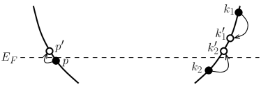
Figure 1: A three-particle process leading to the decay of a quasiparticle in the state $k_{1}$ above the Fermi level involves two additional quasiparticles below the Fermi level, one, $k_{2}$, on the same branch and the other, $p$, on the opposite branch.

The decay rate is then found from Fermi’s golden rule

$$\frac{1}{\tau} = \frac{\pi}{\hbar}\sum_{p,k_{1}^{\prime},k_{2}^{\prime}>0\atop p^{\prime},k_{2}<0}\Big{|}{\mathcal{A}}_{k_{1},k_{2},p}^{k_{1}^{\prime},k_{2}^{\prime},p^{\prime}}\Big{|}^{2}$$ (6)

$$\times\delta(\varepsilon_{k_{1}}+\varepsilon_{k_{2}}+\tilde{\varepsilon}_{p}-\varepsilon_{k_{1}^{\prime}}-\varepsilon_{k_{2}^{\prime}}-\tilde{\varepsilon}_{p^{\prime}}),$$

where the transition matrix element is defined in terms of the $T$-matrix as

$${\mathcal{A}}_{k_{1},k_{2},p}^{k_{1}^{\prime},k_{2}^{\prime},p^{\prime}}=\langle a_{k_{1}^{\prime}}a_{k_{2}^{\prime}}\tilde{a}_{p^{\prime}}|T|\tilde{a}_{p}^{\dagger}a_{k_{2}}^{\dagger}a_{k_{1}}^{\dagger}\rangle.$$ (7)

A three-particle scattering event can be accomplished in the second order in perturbations coupling two particles, such as the term (5). In addition, a contribution to the amplitude (7) can be obtained in the first order in three-particle coupling, which appears in perturbations with scaling dimensions higher than 4.

Because the conservation of momentum imposes restrictions on the final states of the three particles, the matrix element (7) must have the form $\mathcal{A}\delta_{k_{1}+k_{2}+p,k_{1}^{\prime}+k_{2}^{\prime}+p^{\prime}}$. Furthermore, since we are interested in the decay rate of a quasiparticle with small momentum $k_{1}$, and all the other quasiparticles have momenta smaller than $k_{1}$ in absolute value, one may expect to be able to take the limit $k_{1},k_{1}^{\prime},\ldots\to 0$ and replace $\mathcal{A}$ with the resulting constant. This would be incorrect because the quasiparticles on the same branch are identical fermions, and thus the matrix element (7) is antisymmetric with respect to permutations $k_{1}\leftrightarrow k_{2}$ and $k_{1}^{\prime}\leftrightarrow k_{2}^{\prime}$. We therefore conclude that

$${\mathcal{A}}_{k_{1},k_{2},p}^{k_{1}^{\prime},k_{2}^{\prime},p^{\prime}}=\frac{\Lambda}{L^{2}}(k_{1}-k_{2})(k_{1}^{\prime}-k_{2}^{\prime})\delta_{k_{1}+k_{2}+p,k_{1}^{\prime}+k_{2}^{\prime}+p^{\prime}},$$ (8)

where $\Lambda$ is symmetric with respect to the above permutation and takes a constant value at $k_{1}\to 0$. We note that in the limit of weak interactions the three-particle scattering amplitude does have the form (8) at $k_{1}\to 0$, cf. Eq. (47) in Ref. Khodas et al., 2007.

Substituting the scattering amplitude (8) into Eq. (6) we obtain the expression

$$\frac{1}{\tau}=\frac{3}{5120\pi^{3}}\frac{\Lambda^{2}\varepsilon^{8}}{\hbar^{5}m^{*}v^{10}}$$ (9)

for the decay rate of a fermionic quasiparticle with energy $\varepsilon=vk_{1}$. The strong suppression of the quasiparticle decay at low energies, $\tau^{-1}\propto\varepsilon^{8}$, is our main result.

Similar to the decay rate for weakly interacting fermions, the eighth power of energy is a combined effect of the weak scattering amplitude, $|\mathcal{A}|^{2}\propto\varepsilon^{4}$, and small phase space volume for three-particle scattering, $\nu\propto\varepsilon^{4}$ Khodas et al. (2007); Pereira et al. (2009); Ristivojevic and Matveev (2013). The former result is a direct consequence of the Fermi statistics of the quasiparticles, whereas the latter is limited to systems where the quadratic correction to the spectrum (4) is not forbidden by symmetry. For example, the result (9) does not apply to interacting fermions on a tight-binding chain at half filling. Apart from this limitation, our result (9) is rather generic. Most importantly, it is not limited to systems of weakly interacting fermions. In particular, it applies at strong interactions, the so-called Wigner crystal regime, when the Luttinger-liquid parameter $K\ll 1$. One should keep in mind, however, that in this case the description of the system in terms of weakly interacting fermionic excitations is expected to be valid only at particularly small energies $\varepsilon\ll\sqrt{K}\,vp_{F}$ Lin et al. (2013).

The prefactor in our result (9) for the decay rate is expressed in terms of the parameter $\Lambda$ introduced in Eq. (8). A microscopic theory for it can be developed in the limit of weak interactions Khodas et al. (2007); Ristivojevic and Matveev (2013). At arbitrary interaction strength, an analytic microscopic treatment is possible only for integrable models, in which excitations are expected to have infinite lifetimes, i.e., $\Lambda=0$. On the other hand, it is possible to obtain an expression for $\Lambda$ in terms of the parameters $v$, $m^{*}$, and $\lambda$ of the excitation spectrum (4) and their dependences on the density $n$ and momentum per particle $\kappa$ of the liquid.

The most straightforward approach involves identifying the possible perturbations to the Hamiltonian (2) up to the scaling dimension 5 and performing the evaluation of the $T$-matrix up to second order in such perturbations. This is a laborious procedure that will be discussed elsewhere. Here we pursue an alternative approach based on the idea that a quasiparticle can often be treated as a mobile impurity in the Luttinger liquid Ogawa et al. (1992); Castro Neto and Fisher (1996); Khodas et al. (2007); Imambekov and Glazman (2008); Pereira et al. (2009); Schecter et al. (2012); Matveev and Andreev (2012).

Luttinger liquid theory applies only to low-energy properties of the system. Thus its Hamiltonian (1) accounts only for the excitations with energies below certain bandwidth $D$. The exact value of $D$ is usually not important, as long as it is small compared to the characteristic energy scales of the problem, such as the Fermi energy. In our discussion so far the quasiparticles were constructed out of bosonic excitations of the Luttinger liquid, i.e., the quasiparticle energy $\varepsilon\ll D$. Alternatively, one can choose $D\ll\varepsilon$, in which case the quasiparticle is not part of the Luttinger liquid and should be treated as a mobile impurity. Let us consider a special case of the three-particle scattering process (7) for which $k_{2}^{\prime}=-Q$ and $k_{2}=-Q-\delta Q$, where $Q\gg D/v$, and all the remaining momenta are such that $|k_{1}|,|k_{1}^{\prime}|,|p|,|p^{\prime}|\ll D/v$. According to Eq. (8), to leading order in small $\delta Q$, the scattering matrix element for this process is given by

$$\mathcal{A}=\frac{\Lambda}{L^{2}}Q^{2}\,\delta_{q-\tilde{q},\delta Q},$$ (10)

where $q=k_{1}-k_{1}^{\prime}$ and $\tilde{q}=p^{\prime}-p$ are the momenta of the particle-hole pairs collapsed near the right Fermi point and created near the left one, respectively.

Since the particle-hole pairs correspond to bosons of the standard Luttinger liquid theory (1), one can think of this process as scattering of a hole from state $Q$ to $Q+\delta Q$ while absorbing a boson $q$ and emitting a boson $\tilde{q}$. Such processes were studied in Ref. Matveev and Andreev, 2012. The expression for the respective scattering amplitude can be brought to the form Matveev (2013)

$$t_{q,\tilde{q}}=-\frac{\sqrt{|q\tilde{q}|}}{2\pi\hbar L}\,Y_{Q},$$ (11)

with

$$Y_{Q}=\partial^{2}_{LR}\varepsilon_{Q}-\frac{1}{m_{Q}^{*}}\frac{\partial_{L}\varepsilon_{Q}}{v+v_{Q}}\frac{\partial_{R}\varepsilon_{Q}}{v-v_{Q}}+\partial_{L}v_{Q}\frac{\partial_{R}\varepsilon_{Q}}{v-v_{Q}}$$

$$\hskip 5.0pt-\partial_{R}v_{Q}\frac{\partial_{L}\varepsilon_{Q}}{v+v_{Q}}+\frac{v\partial_{n}K}{\sqrt{K}}\bigg{(}\frac{\partial_{R}\varepsilon_{Q}}{v-v_{Q}}+\frac{\partial_{L}\varepsilon_{Q}}{v+v_{Q}}\bigg{)}.$$ (12)

The quasiparticle velocity and mass here depend on momentum, $v_{Q}=\varepsilon_{Q}^{\prime}$ and $1/m_{Q}^{*}=\varepsilon_{Q}^{\prime\prime}$, and the following shorthand notation is used:

$$\partial_{R} = \sqrt{K}\partial_{n}+\frac{\pi\hbar}{\sqrt{K}}\partial_{\kappa},$$ (13a)

$$\partial_{L} = \sqrt{K}\partial_{n}-\frac{\pi\hbar}{\sqrt{K}}\partial_{\kappa},$$ (13b)

$$\partial^{2}_{LR} = K\partial_{n}^{2}-\frac{(\pi\hbar)^{2}}{K}\partial_{\kappa}^{2}.$$ (13c)

Because scattering of the hole by two bosons in the Luttinger liquid is a special case of the three-fermion scattering event, we can use the above result to determine $\Lambda$. To this end, we substitute the $T$-matrix $t_{q,\tilde{q}}\,a_{-Q}^{\dagger}a_{-Q-\delta Q}b_{\tilde{q}}^{\dagger}b_{q}$ into Eq. (7) and use Eq. (3) for the boson operators. The resulting scattering amplitude has the form (10) with $\Lambda=Y_{Q}/Q^{2}$. As expected, at $Q\to 0$ the latter expression has a finite limit

$$\Lambda = \frac{1}{2}\left(\partial^{2}_{LR}\frac{1}{m^{*}}-2\pi\partial_{L}\lambda\right)-\frac{\partial_{L}v}{4v}\partial_{L}\frac{1}{m^{*}}+\frac{(\partial_{L}v)^{2}}{4m^{*}v^{2}}$$ (14)

$$-\left(\frac{\partial_{L}v}{4v}+\frac{m^{*}}{2}\partial_{L}\frac{1}{m^{*}}\right)\left(\partial_{R}\frac{1}{m^{*}}-2\pi\lambda\right).$$

It is worth noting that the absence of the inversion symmetry in the above expression is caused by our choice of the quasiparticle on the right-moving branch.

Expression (14) relates $\Lambda$ to the parameters $v$, $m^{*}$, and $\lambda$ of the quasiparticle spectrum (4) and their dependences on the particle density $n$ and momentum per particle $\kappa$ of the liquid. In combination with Eq. (9) it gives a complete expression for the decay rate of fermionic quasiparticles in a spinless quantum liquid. Our result is valid at any strength of the interactions between the physical particles constituting the liquid. Although our discussion focused on liquids of spinless fermions, the results are also applicable to one-dimensional systems of interacting bosons.

Relaxation of excitations in a one-dimensional system with spins was recently observed in experiment with quantum wires Barak et al. (2010). To test our results, the spins may be polarized by a sufficiently strong in-plane magnetic field. More generally, the decay of quasiparticles may be observed as the broadening of sharp features in the density structure factor or spectral functions. Both types of measurements can, in principle, be performed in experiments with two parallel quantum wires. The density structure factor controls the Coulomb drag in such devices Pustilnik et al. (2003), whereas the spectral functions can be measured in experiments with momentum-resolved tunneling between the wires Auslaender et al. (2005). The same experiments would also measure the excitation spectrum, enabling a quantitative test of our results (9) and (14).

The authors are grateful to L. I. Glazman, M. Pustilnik, and Z. Ristivojevic for helpful discussions. This work was supported by UChicago Argonne, LLC, under contract No. DE-AC02-06CH11357, by JSPS KAKENHI Grant No. 24540338, and by the RIKEN iTHES Project. This work was supported in part by the National Science Foundation under Grant No. PHYS-1066293 and the hospitality of the Aspen Center for Physics.

References

- Landau (1956) L. D. Landau, Sov. Phys. JETP 3, 920 (1956).
- Lifshitz and Pitaevskii (1980) E. M. Lifshitz and L. P. Pitaevskii, Statistical Physics, Part II (Butterworth-Heinemann, 1980).
- Haldane (1981) F. D. M. Haldane, J. Phys. C 14, 2585 (1981).
- Giamarchi (2004) T. Giamarchi, Quantum Physics in One Dimension (Clarendon Press, Oxford, 2004).
- Samokhin (1998) K. V. Samokhin, J. Phys.: Condens. Matter 10, L533 (1998).
- Mattis and Lieb (1965) D. C. Mattis and E. H. Lieb, J. Math. Phys. 6, 304 (1965).
- Rozhkov (2005) A. V. Rozhkov, Eur. Phys. J. B 47, 193 (2005).
- Imambekov et al. (2012) A. Imambekov, T. L. Schmidt, and L. I. Glazman, Rev. Mod. Phys. 84, 1253 (2012).
- Khodas et al. (2007) M. Khodas, M. Pustilnik, A. Kamenev, and L. I. Glazman, Phys. Rev. B 76, 155402 (2007).
- Pereira et al. (2009) R. G. Pereira, S. R. White, and I. Affleck, Phys. Rev. B 79, 165113 (2009).
- Ristivojevic and Matveev (2013) Z. Ristivojevic and K. A. Matveev, Phys. Rev. B 87, 165108 (2013).
- Lin et al. (2013) J. Lin, K. A. Matveev, and M. Pustilnik, Phys. Rev. Lett. 110, 016401 (2013).
- Ogawa et al. (1992) T. Ogawa, A. Furusaki, and N. Nagaosa, Phys. Rev. Lett. 68, 3638 (1992).
- Castro Neto and Fisher (1996) A. H. Castro Neto and M. P. A. Fisher, Phys. Rev. B 53, 9713 (1996).
- Imambekov and Glazman (2008) A. Imambekov and L. I. Glazman, Phys. Rev. Lett. 100, 206805 (2008).
- Schecter et al. (2012) M. Schecter, D. M. Gangardt, and A. Kamenev, Ann. Phys. 327, 639 (2012).
- Matveev and Andreev (2012) K. A. Matveev and A. V. Andreev, Phys. Rev. B 86, 045136 (2012).
- Matveev (2013) K. A. Matveev, J. Exp. Theor. Phys. 117, 508 (2013).
- Barak et al. (2010) G. Barak, H. Steinberg, L. N. Pfeiffer, K. W. West, L. Glazman, F. von Oppen, and A. Yacoby, Nat. Phys. 6, 489 (2010).
- Pustilnik et al. (2003) M. Pustilnik, E. G. Mishchenko, L. I. Glazman, and A. V. Andreev, Phys. Rev. Lett. 91, 126805 (2003).
- Auslaender et al. (2005) O. M. Auslaender, H. Steinberg, A. Yacoby, Y. Tserkovnyak, B. I. Halperin, K. W. Baldwin, L. N. Pfeiffer, and K. W. West, Science 308, 88 (2005).