A New Decomposition Method for Multiuser DC-Programming and its Applications

Abstract

We propose a novel decomposition framework for the distributed optimization of Difference Convex (DC)-type nonseparable sum-utility functions subject to coupling convex constraints. A major contribution of the paper is to develop for the first time a class of (inexact) best-response-like algorithms with provable convergence, where a suitably convexified version of the original DC program is iteratively solved. The main feature of the proposed successive convex approximation method is its decomposability structure across the users, which leads naturally to distributed algorithms in the primal and/or dual domain. The proposed framework is applicable to a variety of multiuser DC problems in different areas, ranging from signal processing, to communications and networking.

As a case study, in the second part of the paper we focus on two examples, namely: i) a novel resource allocation problem in the emerging area of cooperative physical layer security; ii) and the renowned sum-rate maximization of MIMO Cognitive Radio networks. Our contribution in this context is to devise a class of easy-to-implement distributed algorithms with provable convergence to stationary solution of such problems. Numerical results show that the proposed distributed schemes reach performance close to (and sometimes better than) that of centralized methods.

I Introduction

The resource allocation problem in multiuser systems generally consists of optimizing the (weighted) sum of the users’ objective functions, also termed a “social function”. In this paper we address the frequent and difficult case in which the social function is nonconvex and there are (convex) shared constraints coupling the strategies of all the users. Our attention is mainly focused on objective functions of the DC-type, i.e., the difference of two convex functions. It is worth mentioning that DC programs are very common in signal processing, communications, and networking. For instance, the following resource allocation problems belong to the class of DC programs: power control problems in cellular systems [1, 2, 3]; MIMO relay optimization [4]; dynamic spectrum management in DSL systems [5, 6]; sum-rate maximization, proportional-fairness and max-min optimization of SISO/MISO/MIMO ad-hoc networks [7, 8, 9, 10].

In the effort of (optimally) solving DC programs, a great deal of the aforementioned works involves global optimization techniques whose solution methods are mainly based on combinatorial approaches (e.g., adaptations of branch and bound techniques [11]); the results are a variety of centralized algorithms customized to the specific DC structure under considerations [1, 5, 2, 3, 4]. However, centralized schemes are too demanding in most applications (e.g., large-scale decentralized networks). This has motivated a number of works whose effort has been finding efficiently high quality (generally locally optimal) solutions of DC programs via easy-to-implement distributed algorithms. Distributed ad-hoc schemes (with provable convergence) for very specific DC formulations have been proposed in [8, 7, 10, 6], mainly based on Successive Convex Approximation (SCA) techniques [10, 12, 13]. In these works however the formulations contain only private constraints (i.e., there is no coupling among the users’ strategies).

In this paper, we move a step forward and consider the more general multiuser DC program, whose feasible set includes also coupling convex constraints. To the best of our knowledge, the design of distributed algorithms for this class of problems is an open issue. Indeed, the nonconvexity of the social function prevents the application of standard primal/dual decomposition techniques for convex problems, e.g., [14, 15]; the presence of coupling constraints makes the distributed techniques developed in [8, 7, 10, 6, 12] not directly usable; and standard SCA methods for DC programs [13] wherein the concave part of the objective function is linearized would lead to centralized schemes (because the resulting convex function is generally not separable in the users’ variables).

A first contribution of this paper is to develop a novel distributed decomposition method for solving such a class of multiuser DC problems. Capitalizing on the SCA idea, the proposed novel technique solves a sequence of strongly convex subproblems, whose objective function is obtained by diagonalization plus off-diagonal linearization of the convex part of the original DC sum-utility and linearization of the nonconvex part. Some desirable features of the proposed approach are: i) Convergence to a stationary solution of the original DC programming is guaranteed also if the subproblems are solved in an inexact way; ii) Each convex subproblem can be distributively solved by the users capitalizing on standard primal or dual decomposition techniques; and iii) It leads to alternative distributed algorithms that differ from rate and robustness of convergence, scalability, local computation versus global communication, and quantity of message passing. All these features make the proposed technique and algorithms applicable to a variety of networks scenarios and problems.

As a case study, in the second part of the paper we show how to customize the developed framework to two specific problems, namely: 1) a novel resource allocation problem in the emerging area of cooperative physical layer security; and 2) the renowned sum-rate maximization of MIMO Cognitive Radio (CR) networks. A brief description of our main contributions in these two contexts is given next.

I-1 Cooperative physical layer security

Physical layer security has been considered as a promising technique to prevent illegitimate receivers from eavesdropping on the confidential message transmitted between intended network nodes; see, e.g., [16] and references therein. Recently, cooperative transmissions using trusted relays or friendly jammers to improve physical layer security has attracted increasing attention [17, 18, 19, 20, 21, 22, 23, 24]. Of particular interest to this work is the Cooperative Jamming (CJ) paradigm (see, e.g., [17, 18, 19]): friendly jammers create judicious interference by transmitting noise (or codewords) so as to impair the eavesdropper’s ability to decode the confidential information, and thus, increase secure communication rates between legitimate parties. The interference from the jammers however might also reduce the useful rate of the legitimate links; therefore the maximization of the users’ secrecy rate calls for a joint optimization of the power allocations of the sources and the jammers.

In this paper we address such a joint optimization problem. We consider a network model composed of multiple transmitter-receiver pairs, multiple friendly jammers, and a single eavesdropper. Note that previous works studied simpler system models, composed of either one source-destination link (and possibly multiple jammers) or multiple sources but one jammer. We formulate the system design as a game wherein the players$-$the legitimate users$-$maximize their own secrecy rate by choosing jointly their transmit power and (the optimal fraction of the) power of the friendly jammers. The resulting secrecy game faces two main challenges, namely: i) the players’ objective functions are nonconcave and nondifferentiable; and ii) there are side (thus coupling) constraints. All this makes the analysis of the proposed game a difficult task; for instance, a Nash Equilibrium may not even exist. Capitalizing on recent results on nonconvex games with side constraints [25, 26], we introduce a novel relaxed equilibrium concept for the nonconvex nondifferentiable game, named (restricted) B-Quasi Generalized Nash Equilibrium (B-QGNE). Roughly speaking a B-QGNE is a solution of the first order aggregated stationarity conditions (based on directional derivatives) of the players’ optimization problems. Aiming to devise distributed algorithms computing a (B-)QGNE, we establish a connection between (a subclass of) such equilibria and the stationary solutions of a suitably defined differentiable DC program with side constraints, for which we can successfully use the DC framework developed in the first part of the paper. To the best of our knowledge, this is the first attempt toward a rigorous characterization of the nondifferentiability issue in secrecy capacity multiuser resource allocation problems. Numerical experiments show that the proposed distributed algorithms yield sum-secrecy-rates that are better than those achievable by centralized schemes (attempting to compute stationary solutions of the DC program), and comparable to those achievable by computationally expensive techniques attempting to obtain globally optimal solutions.

I-2 MIMO Cognitive Radio design

We consider the sum-rate maximization of CR MIMO systems, subject to coupling interference constraints. Special cases of such a nonconvex problem have been widely studied in the literature. The analysis is mainly limited to local interference constraints (see [8, 27] and references therein), with the exception of [7, 28] where coupling constraints are considered. However the theoretical convergence of algorithms in [7, 28] is up to date an open problem. Since the general optimization problem is an instance of DC programs with shared constraints, we can apply the framework developed in the paper and obtain for the first time a class of distributed (primal/dual-based) algorithms with probable convergence.

In summary, the main contributions of this paper are:

$\bullet$ A novel class of distributed decomposition algorithms with provable convergence for multiuser DC problems with (convex) side constraints.

$\bullet$ A novel game theoretical formulation for the secrecy rate maximization problem in multiple source-destination OFDMA networks with multiple friendly jammers, and consequent algorithms to compute its QGNE based on a nontrivial DC reformulation of the game.

$\bullet$ A class of provable convergent distributed primal/dual algorithms for the CR MIMO sum-rate maximization problem.

The rest of this paper is organized as follows. Section II introduces the proposed multiuser DC problem with coupling constraints. Section III presents a novel decomposition technique for computing stationary solutions of the DC problem, which is suitable for a distributed implementation. Distributed algorithms building on primal and dual decomposition techniques are discussed in Section IV. Section V customizes the proposed framework to the cooperative physical layer security game and the CR MIMO sum-rate maximization problem. Finally, Section VI draws some conclusions.

II Multiuser DC-Program with side constraints

We consider a multiuser system composed of $I$ coupled users. Each user $i$ makes decision on his $n_{i}$-dimensional real strategy vector $\mathbf{x}_{i}\in\mathbb{R}^{n_{i}}$, subject to some local constraints given by the set $\mathcal{X}_{i}\subset\mathbb{R}^{n_{i}}$. The joint strategy set is denoted by $\mathcal{X}\triangleq{\prod_{i=1}^{I}\mathcal{X}_{i}}$; $\mathbf{x}_{-i}\triangleq(\mathbf{x}_{j})_{j\neq i}$ is the strategy vector of all users except user $i$; $\mathcal{X}_{-i}\triangleq{\prod_{j\neq i}\mathcal{X}_{j}}$; and $\mathbf{x}\triangleq(\mathbf{x}_{i})_{i=1}^{I}$ denotes the strategy profile of all the users. In addition to the private constraints, there are also side constraints in the form of a $n_{c}$-vector function $\mathbf{h}(\mathbf{x})\triangleq(h_{j}(\mathbf{x}))_{j=1}^{n_{c}}\leq\mathbf{0}$. The system design is formulated as a DC program in the following form:

$$\begin{array}[]{ll}\underset{\mathbf{x}}{\text{minimize}}&\theta(\mathbf{x})\triangleq{\displaystyle\sum_{i=1}^{I}\left(f_{i}(\mathbf{x})-g_{i}(\mathbf{x})\right)}\vskip 3.0pt plus 1.0pt minus 1.0pt\\ \text{subject to }&\mathbf{x}_{i}\in\mathcal{X}_{i}\,\,\,\,\,\forall\,i=1,\ldots,I\,\,\text{(private constraints)}\vskip 6.0pt plus 2.0pt minus 2.0pt\\ &\mathbf{h}(\mathbf{x})\leq\mathbf{0}\hfill\,\,\,\,\,\,\,\,\text{(coupling constraints)}.\end{array}$$ (1)

Assumptions. We make the following blanket assumptions:

A1) The functions $f_{i}$, $g_{i}$ for $i=1,\ldots,I$, and $h_{j}$ for $j=1,\ldots,n_{c}$, are convex and continuously differentiable on $\mathcal{X}$;

A2) Each set $\mathcal{X}_{i}$ is (nonempty) closed and convex;

A3) The functions $f_{i}$ and $g_{i}$ have Lipschitz continuous gradients on $\Xi$ with constant $L_{\nabla f_{i}}$ and $L_{\nabla g_{i}}$, respectively; where $\Xi$ denotes the convex feasible set of (1); let $L_{\nabla\theta}\triangleq\sum_{i}L_{\nabla f_{i}}+\sum_{i}L_{\nabla g_{i}}$.

A4) The lower level set $\mathcal{L}(\mathbf{x}^{0})\triangleq\left\{\mathbf{x}\in\Xi\,|\,\theta(\mathbf{x})\leq\theta(\mathbf{x}^{0})\right\}$ of the objective function $\theta$ is compact for some $\mathbf{x}^{0}\in\Xi$;

A5) The convex coupling constraints are in the separable form: $\mathbf{h}(\mathbf{x})\triangleq\sum_{i=1}^{I}\mathbf{h}_{i}(\mathbf{x}_{i})\leq\mathbf{0}$.

The assumptions above are quite standard and are satisfied by a large class of practical problems. For instance, A4 guarantees that (1) has a solution even when $\Xi$ is not bounded; of course A4 is trivially satisfied if $\Xi$ is bounded.

Instances of problem (1) appear in many applications, from signal processing to communications and networking; see Sec. V for some motivating examples. Our goal is to obtain distributed best-response-like algorithms for the class of problems (1), converging to stationary solutions. This confronts three major challenges, namely: i) the objective function is the sum of differences of two convex functions, and thus in general nonconvex; ii) the objective function is not separable in the users’ strategies (each function $f_{i}$ and $g_{i}$ depends on the strategy profile $\mathbf{x}$ of all users); and iii) there are side constraints coupling all the optimization variables. We deal with these issues in the following sections.

III A new best-response SCA decomposition

The standard SCA-based technique for DC programs applied to (1) would suggest solving a sequence of convex subproblems whose objective function is obtained by linearizing at the current iterate the nonconvex part of $\theta(\mathbf{x})$, that is $\sum_{i}g_{i}(\mathbf{x})$, while retaining the convex part $\sum_{i}f_{i}(\mathbf{x})$; see, e.g., [13, 12]. However, because of the nonseparability of the aforementioned terms, the resulting convexification does not enjoy a decomposable structure; therefore such SCA techniques will lead to centralized solution methods.

Here we introduce a new decomposition technique that does not suffer from this drawback. To formally describe our approach, let us start rewriting each function $f_{i}(\mathbf{x})$ as: given $\mathbf{x}^{\nu}$ and denoting $\mathbf{x}_{-i}^{\nu}\triangleq\left(\mathbf{x}_{j}^{\nu}\right)_{j\neq i}$, we have

$$f_{i}(\mathbf{x})=f_{i}(\mathbf{x}_{i},\mathbf{x}_{-i}^{\nu})+\left[f_{i}(\mathbf{x}_{i},\mathbf{x}_{-i})-f_{i}(\mathbf{x}_{i},\mathbf{x}_{-i}^{\nu})\right].$$ (2)

We now approximate the term in brackets using a first order Taylor expansion at $\mathbf{x}^{\nu}$,

$$f_{i}(\mathbf{x}_{i},\mathbf{x}_{-i})-f_{i}(\mathbf{x}_{i},\mathbf{x}_{-i}^{\nu})\approx\sum_{j\neq i}\nabla_{\mathbf{x}_{j}}f_{i}(\mathbf{x}^{\nu})^{T}(\mathbf{x}_{j}-\mathbf{x}_{j}^{\nu}),\vspace{-0.2cm}$$

and approximate (2) as

$$f_{i}(\mathbf{x})\approx\widetilde{{f}}_{i}(\mathbf{x};\mathbf{x}^{\nu})\triangleq\underbrace{f_{i}(\mathbf{x}_{i},\mathbf{x}_{-i}^{\nu})}_{\text{diagonalization }}+\underbrace{\sum_{j\neq i}\nabla_{\mathbf{x}_{j}}f_{i}(\mathbf{x}^{\nu})^{T}(\mathbf{x}_{j}-\mathbf{x}_{j}^{\nu})}_{\text{off-diagonal linearization}}$$ (3)

yielding a diagonalization plus off-diagonal linearization of $f_{i}(\mathbf{x})$ at $\mathbf{x}^{\nu}$. To deal with the nonconvexity of $-g_{i}(\mathbf{x})$, we replace the functions $g_{i}(\mathbf{x})$ with its linearization at $\mathbf{x}^{\nu}$:

$$g_{i}(\mathbf{x})\approx\widetilde{{g}}_{i}(\mathbf{x};\mathbf{x}^{\nu})\triangleq\underbrace{g_{i}(\mathbf{x}^{\nu})+\sum_{j=1}^{I}\nabla_{\mathbf{x}_{j}}g_{i}(\mathbf{x}^{\nu})^{T}(\mathbf{x}_{j}-\mathbf{x}_{j}^{\nu})}_{\text{linearization}}.\vspace{-0.1cm}$$ (4)

Based on (3) and (4), the candidate approximation of the nonconvex sum-utility $\theta(\mathbf{x})$ at $\mathbf{x}^{\nu}$ is:

$$\widetilde{{\theta}}(\mathbf{x};\mathbf{x}^{\nu})\triangleq\sum_{i=1}^{I}\left(\widetilde{{f}}_{i}(\mathbf{x};\mathbf{x}^{\nu})-\widetilde{{g}}_{i}(\mathbf{x};\mathbf{x}^{\nu})\right)+\sum_{i=1}^{I}\frac{\tau_{i}}{2}\|\mathbf{x}_{i}-\mathbf{x}_{i}^{\nu}\|^{2},$$ (5)

where we added a proximal-like regularization term with $\tau_{i}\geq 0$, whose numerical benefits are well-understood; see, e.g., [14]. Rearranging the terms in the above sum, it is not difficult to see that (5) can be equivalently rewritten as

$$\widetilde{{\theta}}(\mathbf{x};\mathbf{x}^{\nu})=\sum_{i=1}^{I}\widetilde{{\theta}}_{i}(\mathbf{x}_{i};\mathbf{x}^{\nu}),$$ (6)

where

$$\widetilde{{\theta}}_{i}(\mathbf{x}_{i};\mathbf{x}^{\nu})\triangleq\left[f_{i}(\mathbf{x}_{i},\mathbf{x}_{-i}^{\nu})+\sum_{j\neq i}\nabla_{\mathbf{x}_{i}}f_{j}(\mathbf{x}^{\nu})^{T}(\mathbf{x}_{i}-\mathbf{x}_{i}^{\nu})\right]$$ (7)

$$-\left[g_{i}(\mathbf{x}^{\nu})+\sum_{j=1}^{I}\nabla_{\mathbf{x}_{i}}g_{j}(\mathbf{x}^{\nu})^{T}(\mathbf{x}_{i}-\mathbf{x}_{i}^{\nu})\right]+\frac{\tau_{i}}{2}\|\mathbf{x}_{i}-\mathbf{x}_{i}^{\nu}\|^{2}.$$

Roughly speaking, the main idea behind the above approximations is to use a proper combination of diagonalization and partial linearization on the convex functions $f_{i}(\mathbf{x})$ [cf. (3)] together with a linearization of the nonconvex terms $g_{i}(\mathbf{x})$ [cf. (4)]. The diagonalization procedure fixes the non-separability issue in $\theta(\mathbf{x})$ while preserving the convex part in $\theta(\mathbf{x})$, whereas the linearization of $g_{i}(\mathbf{x})$ gets rid of the nonconvex part in $\theta(\mathbf{x})$. Indeed, this procedure leads to the approximation function $\widetilde{{\theta}}(\mathbf{x};\mathbf{x}^{\nu})$ at $\mathbf{x}^{\nu}$ that is separable in the users’ variables $\mathbf{x}_{i}$ [each $\widetilde{{\theta}}_{i}(\mathbf{x}_{i};\mathbf{x}^{\nu})$ depends only on $\mathbf{x}_{i}$, given $\mathbf{x}^{\nu}$] and is strongly convex in $\mathbf{x}\in\Xi$.

The proposed SCA decomposition consists then in solving iteratively (possibly with a memory) the following sequence of (strongly) convex optimization problems: given $\mathbf{x}^{\nu}\in\Xi$,

$$\widehat{\mathbf{x}}\left(\mathbf{x}^{\nu}\right)\triangleq\underset{\mathbf{x}\in\Xi}{\text{argmin}}\,\,\,\widetilde{{\theta}}(\mathbf{x};\mathbf{x}^{\nu}).$$ (8)

The formal description of the proposed SCA technique is given in Algorithm 1. Note that in Step 3 of the algorithm we allow a memory in the update of the iterate $\mathbf{x}^{\nu}$ in the form of a convex combination via $\gamma^{\nu}\in(0,1]$ (this guarantees $\mathbf{x}^{\nu+1}\in\Xi$).

Data: $\bm{{\tau}}\triangleq(\tau_{i})_{i=1}^{I}\geq\mathbf{0},\{\gamma^{\nu}\}>0$ and $\mathbf{x}^{0}\in\Xi$. Set $\nu=0$.

$(\texttt{S.1})$: If $\mathbf{x}^{\nu}$ satisfies a termination criterion, STOP;

$(\texttt{S.2})$: Compute $\widehat{\mathbf{x}}\left(\mathbf{x}^{\nu}\right)$ [cf. (8)];

$(\texttt{S.3})$: Set $\mathbf{x}^{\nu+1}\triangleq\mathbf{x}^{\nu}+\gamma^{\nu}\left(\,\widehat{\mathbf{x}}\left(\mathbf{x}^{\nu}\right)-\mathbf{x}^{\nu}\,\right)$;

$(\texttt{S.4})$: $\nu\leftarrow\nu+1$ and go to $(\texttt{S.1})$.

Algorithm 1 : SCA Algorithm for the DC program (1)

The convergence of the algorithm is studied in the next theorem, where $c_{f_{i}}(\mathbf{x}_{-i})\geq 0$ in (10) is the largest constant such that $(\mathbf{z}_{i}-\mathbf{w}_{i})^{T}(\nabla_{\mathbf{x}_{i}}f_{i}(\mathbf{z}_{i},\mathbf{x}_{-i})-\nabla_{\mathbf{x}_{i}}f_{i}(\mathbf{w}_{i},\mathbf{x}_{-i}))\geq c_{f_{i}}(\mathbf{x}_{-i})\|\mathbf{z}_{i}-\mathbf{w}_{i}\|^{2},$ for all $\mathbf{z}_{i},\mathbf{w}_{i}\in\mathcal{X}_{i}$ and $\mathbf{x}_{-i}\in\mathcal{X}_{-i}$.

Theorem 1.

Given the DC program (1) under A1-A4, suppose that $\bm{{\tau}}\triangleq(\tau_{i})_{i=1}^{I}$ and $\{\gamma^{\nu}\}$ are chosen so that one of the two following conditions are satisfied:

(a) Constant step-size rule:

$$\gamma^{\nu}=\gamma\in(0,1]\,\,\,\,\forall\,\nu\geq 0\,\,\,\,\text{ and }\,\,\,\,2\,c_{\bm{{\tau}}}>\gamma L_{\nabla\theta}.$$ (9)

with

$$c_{\bm{{\tau}}}\triangleq\min_{i=1,\ldots,I}\left\{\tau_{i}+\inf_{\mathbf{z}_{-i}\in\mathcal{X}_{-i}}c_{f_{i}}(\mathbf{z}_{-i})\right\}.$$ (10)

(b) Diminishing step-size rule:

$$c_{\bm{{\tau}}}>0,\,\,\,\gamma^{\nu}\in(0,1],\,\,\gamma^{\nu}\rightarrow 0,\,\,\mbox{and}\,\,\,{\textstyle\sum_{\nu=0}^{\infty}\gamma^{\nu}=+\infty.}$$ (11)

Then, the sequence $\{\mathbf{x}^{\nu}\}$ generated by Algorithm 1 converges in a finite number of iterations to a stationary point of (1) or every limit point of the sequence (at least one such point exists) is a stationary solution of (1).

Proof:

See Appendix A. ∎

Remark 1 (On Algorithm 1).

The algorithm implements a novel SCA decomposition technique: at each iteration $\nu$, a separable (strongly) convex function $\widetilde{{\theta}}(\mathbf{x};\mathbf{x}^{\nu})$ is minimized over the convex set $\Xi$. The main difference from the classical SCA techniques (e.g., [11, 13, 12]) is that the approximation function $\widetilde{{\theta}}(\mathbf{x};\mathbf{x}^{\nu})$ is separable across the users. In Section IV, we show that such a structure leads naturally to a distributed implementation of Algorithm 1. A practical termination criterion in Step 1 is to stop the iterates when $|{\theta}(\mathbf{x}^{\nu})-{\theta}(\mathbf{x}^{\nu-1})|\leq\delta$, where $\delta$ is a prescribed accuracy. Finally, it is reasonable to expect the algorithm to perform better than classical gradient algorithms applied directly to (1) at the cost of no extra signaling, because the structure of the objective function ${\theta}(\mathbf{x})$ is better explored.

Remark 2 (On the choice of the free parameters).

Theorem 1 offers some flexibility in the choice of ${\bm{\tau}}$ and $\gamma^{\nu}$, while guaranteeing convergence of Algorithm 1, which makes it applicable in a variety of scenarios. More specifically, one can use a constant or a diminishing rule for the step-size $\gamma^{\nu}$.

Constant step-size rule: This rule resembles analogous constant step-size rules in gradient algorithms: convergence is guaranteed either under “sufficiently” small step-size $\gamma$ (given $\bm{{\tau}}$) or “sufficiently” large $\tau_{i}$’s (given $\gamma\in(0,1]$), such that (9) is satisfied. A special case that is worth mentioning is: $\gamma=1$ and $2\,c_{\bm{{\tau}}}>\gamma L_{\nabla\theta}$, which leads to a SCA-based iterate with no memory: given $\mathbf{x}^{\nu}\in\Xi$, $\mathbf{x}^{\nu+1}\,\triangleq\,\widehat{\mathbf{x}}\left(\mathbf{x}^{\nu}\right)$. In this particular case, we can relax a bit the convergence condition (9) and require the Lipschitz continuity of the gradients of $f_{i}$ only. The result is stated next (see attached material for the proof).

Theorem 2.

Let $\{\mathbf{x}^{\nu}\}$ be the sequence generated by Algorithm 1, in the setting of Theorem 1 where however we relax A3 by assuming that $f_{i}$ have Lipschitz gradients with constants $L_{\nabla f_{i}}$. Suppose that $\gamma^{\nu}=1$ and $\bm{\tau}>\mathbf{0}$ is such that $\tau^{\min}\triangleq\min_{i}\tau_{i}>2\sum_{i=1}^{I}L_{\nabla f_{i}}$; then, the conclusions of Theorem 1 hold.

Diminishing step-size rule: The application of a constant step-size rule requires the knowledge of the Lipschitz constants $L_{\nabla f_{i}}$ and $L_{\nabla g_{i}}$, which may not be available. One can use a (conservative) estimate of such values (e.g., using upper bounds), but in practice this generally leads to “large” values of $c_{\bm{{\tau}}}$ satisfying (9), which reasonably slows down the algorithm. In all these situations, a valid alternative is to use a diminishing step-size in the form (11); examples of such rules are [10]: given $\gamma^{0}=1$,

Rule 1: $$\gamma^{\nu}=\gamma^{\nu-1}\left(1-\epsilon\,\gamma^{\nu-1}\right), \,\nu=1,\ldots,$$ (12)

Rule 2: $$\gamma^{\nu}=\frac{\gamma^{\nu-1}+\beta_{1}}{1+\beta_{2}\nu}, \,\nu=1,\ldots,$$ (13)

where $\epsilon\in(0,1)$ and $\beta_{1},\beta_{2}\in(0,1)$ are given constants such that $\beta_{1}\leq\beta_{2}$.

III-A Inexact implementation of $\widehat{\mathbf{x}}\left(\mathbf{x}^{\nu}\right)$

We can reduce the computational effort of Algorithm 1 by allowing inexact computations of the solution $\widehat{\mathbf{x}}\left(\mathbf{x}^{\nu}\right)$. The convergence of the resulting algorithm is still guaranteed under more stringent conditions on the step-size and some requirements on the computational errors. The inexact version of Algorithm 1 is formally described in Algorithm 2 below, where Step 2 of Algorithm 1, the exact computation of $\widehat{\mathbf{x}}\left(\mathbf{x}^{\nu}\right)$, is replaced now with its inexact version, that is find a $\mathbf{z}^{\nu}$ such that $\|\mathbf{z}^{\nu}-\widehat{\mathbf{x}}\left(\mathbf{x}^{\nu}\right)\|\leq\varepsilon^{\nu}$, with $\varepsilon^{\nu}$ being the accuracy in the computation of $\widehat{\mathbf{x}}\left(\mathbf{x}^{\nu}\right)$ at iteration $\nu$.

Data: $\bm{{\tau}}\geq\mathbf{0},\{\gamma^{\nu}\}>0,\{\varepsilon^{\nu}\}\downarrow 0$, and $\mathbf{x}^{0}\in\Xi$. Set $\nu=0$.

$(\texttt{S.1})$: If $\mathbf{x}^{\nu}$ satisfies a termination criterion, STOP;

$(\texttt{S.2})$: Find a $\mathbf{z}^{\nu}$ such that $\|\mathbf{z}^{\nu}-\widehat{\mathbf{x}}\left(\mathbf{x}^{\nu}\right)\|\leq\varepsilon^{\nu}$;

$(\texttt{S.3})$: Set $\mathbf{x}^{\nu+1}\triangleq\mathbf{x}^{\nu}+\gamma^{\nu}\left(\,\mathbf{z}^{\nu}-\mathbf{x}^{\nu}\,\right)$;

$(\texttt{S.4})$: $\nu\leftarrow\nu+1$ and go to $(\texttt{S.1})$.

Algorithm 2 : Inexact version of Algorithm 1

Convergence is guaranteed if the error sequence $\{\varepsilon^{\nu}\}$ and the step-size $\{\gamma^{\nu}\}$ are properly chosen, as stated in Theorem 3. The proof of this result is based on the application of Proposition 4 (cf. Appendix A) and [10, Th. 4], and is omitted.

Theorem 3.

Let $\{\mathbf{x}^{\nu}\}$ be the sequence generated by Algorithm 2 in the setting of Theorem 1, where however A4 is strengthened by assuming that $\theta$ is coercive on $\Xi$. Suppose that $\{\gamma^{\nu}\}$ and $\{\varepsilon^{\nu}\}$ are chosen so that the following conditions are satisfied: i) $\gamma^{\nu}\in(0,1]$; ii) $\gamma^{\nu}\rightarrow 0$; iii) ${\textstyle{\sum_{\nu=0}^{\infty}\gamma^{\nu}}=+\infty}$; iv) $\sum_{\nu=0}^{\infty}\left(\gamma^{\nu}\right)^{2}<+\infty$; and v) ${\sum_{\nu=0}^{\infty}\varepsilon^{\nu}\,\gamma^{\nu}<+\infty}$. Then, conclusions of Theorem 1 hold.

Note that the steps-size rule in (12) satisfies the square summability condition in Theorem 3. As expected, in the presence of errors, convergence of Algorithm 2 is guaranteed if $\varepsilon^{\nu}\rightarrow 0$, meaning that the sequence of approximated problems (8) is solved with increasing accuracy. Note that Theorem 3v) imposes also a constraint on the rate by which $\varepsilon^{\nu}$ goes to zero, which depends also on $\{\gamma^{\nu}\}$. An example of an error sequence satisfying condition v) is $\varepsilon^{\nu}\leq\alpha\,\gamma^{\nu}$, where $\alpha$ is any finite positive constant. Interestingly, such a condition can be enforced in Algorithm 2 using classical error bound results in convex analysis; see, e.g., [29, Ch. 6]. Two examples of error bounds are given in Lemma 1 below, where we introduced the following residual quantities:

$$r_{\Xi}(\mathbf{z};\mathbf{x}^{\nu}) \triangleq \left\|\Pi_{\mathcal{N}(\mathbf{z},\Xi)}(-\nabla_{\mathbf{x}}\widetilde{{\theta}}(\mathbf{z};\mathbf{x}^{\nu}))+\nabla_{\mathbf{x}}\widetilde{{\theta}}(\mathbf{z};\mathbf{x}^{\nu})\right\|$$

$$l_{\Xi}(\mathbf{z};\mathbf{x}^{\nu}) \triangleq \left\|\mathbf{z}-\Pi_{\Xi}\left(\mathbf{z}-\nabla_{\mathbf{x}}\widetilde{{\theta}}(\mathbf{z};\mathbf{x}^{\nu})\right)\right\|\vspace{-0.1cm}$$

with $\Pi_{\mathcal{N}(\mathbf{z},\Xi)}(\mathbf{y})$ [resp. $\Pi_{\Xi}(\mathbf{y})$] denoting the Euclidean projection of $\mathbf{y}$ onto the normal cone $\mathcal{N}(\mathbf{z},\Xi)\triangleq\{\mathbf{y}\in\mathbb{R}^{n}:\mathbf{y}^{T}(\mathbf{x}-\mathbf{z})\leq 0,\,\forall\mathbf{x}\in\Xi\}$ (resp. $\Xi$). The proof of Lemma 1 is similar to that of [29, Prop. 6.3.1, Prop. 6.3.7] and is omitted.

Lemma 1.

Given the optimization problem (8) under assumptions A1-A4, the following hold:

(a): A (finite) constant $\xi_{1}>0$ exists such that

$$\|\mathbf{z}-\widehat{\mathbf{x}}\left(\mathbf{x}^{\nu}\right)\|\leq\xi_{1}\,r_{\Xi}(\mathbf{z};\mathbf{x}^{\nu}),\quad\mathbf{z}\in\Xi;$$

(b): A (finite) constant $\xi_{2}>0$ exists such that

$$\|\mathbf{z}-\widehat{\mathbf{x}}\left(\mathbf{x}^{\nu}\right)\|\leq\xi_{2}\,l_{\Xi}(\mathbf{z};\mathbf{x}^{\nu}),\quad\mathbf{z}\in\mathbb{R}^{n}.$$

Note that, for a non-polyhedral finitely representable (convex) set $\Xi$ and $\mathbf{z}$, the computation of $l_{\Xi}(\mathbf{z};\mathbf{x}^{\nu})$ amounts to solving a convex optimization problem; whereas in the same case if $\mathbf{z}\in\Xi$ satisfies a suitable Constraint Qualification (CQ), the computation of $r_{\Xi}(\mathbf{z};\mathbf{x}^{\nu})$ reduces to solving a convex quadratic program. Thus $r_{\Xi}(\mathbf{z};\mathbf{x}^{\nu})$ is computationally easier than $l_{\Xi}(\mathbf{z};\mathbf{x}^{\nu})$ to be obtained but, contrary to $l_{\Xi}(\mathbf{z};\mathbf{x}^{\nu})$, it can be used only to test vectors $\mathbf{z}$ belonging to $\Xi$. Using the error bounds in Lemma 1 and given a step-size rule $\{\gamma^{\nu}\}$, the termination criterion in Step 2 of the algorithm becomes then $r_{\Xi}(\mathbf{z};\mathbf{x}^{\nu})\leq\widetilde{{\alpha}}\,\gamma^{\nu}$ or $l_{\Xi}(\mathbf{z};\mathbf{x}^{\nu})\leq\widetilde{{\alpha}}\,\gamma^{\nu}$, for some $\widetilde{{\alpha}}>0$.

III-B Generalizations

So far we have restricted our attention to optimization problems in the DC form. However, it is worth mentioning that the proposed analysis and resulting algorithms (also those introduced in the forthcoming sections) can be readily extended to other sum-utility functions not necessarily in the DC form, such as $\widehat{{\theta}}(\mathbf{x})\triangleq\sum_{\ell\in\mathcal{I}_{f}}{f}_{\ell}(\mathbf{x})$, where the set $I_{f}\triangleq\{1,\ldots,I_{f}\}$ may be different from the set of users $\{1,\ldots,I\}$, and each function ${f}_{\ell}$ is not necessarily expressed as the difference of two convex functions. It is not difficult to show that in such a case the candidate approximation function $\widetilde{{\theta}}(\mathbf{x};\mathbf{x}^{\nu})$ still has the form in (6), where each $\widetilde{{\theta}}_{i}(\mathbf{x};\mathbf{x}^{\nu})$ is now given by

$$\widetilde{{\theta}}_{i}(\mathbf{x};\mathbf{x}^{\nu}) \triangleq\sum_{j\in\mathcal{C}_{i}}f_{j}(\mathbf{x}_{i},\,\mathbf{x}_{-i}^{\nu})+\sum_{j\notin\mathcal{C}_{i}}\nabla_{\mathbf{x}_{i}}f_{j}(\mathbf{x}^{\nu})^{T}(\mathbf{x}_{i}-\mathbf{x}_{i}^{\nu})$$

$$\quad+\frac{\tau_{i}}{2}\|\mathbf{x}_{i}-\mathbf{x}_{i}^{\nu}\|^{2}$$

where $\mathcal{C}_{i}$ is any subset of $\mathcal{S}_{i}\subseteq\mathcal{I}_{f}$, with $\mathcal{S}_{i}\triangleq\left\{j\in\mathcal{I}_{f}\!:\!f_{j}(\bullet,\mathbf{x}_{-i})\,\mbox{is convex on }\mathcal{X}_{i},\forall\mathbf{x}_{-i}\in\mathcal{X}_{-i}\right\}$. In $\widetilde{{\theta}}_{i}(\mathbf{x};\mathbf{x}^{\nu})$ each user linearizes only the functions outside $\mathcal{C}_{i}$ while preserving the convex part of the sum-utility. The choice of $\mathcal{C}_{i}\subseteq\mathcal{S}_{i}$ is a degree of freedom useful to explore the tradeoff between signaling and convergence speed. We omit further details because of space limitation.

IV Distributed Implementation

In general, the implementation of Algorithms 1 and 2 requires a coordination among the users; the amount of network signaling depends on the specific application under consideration. To alleviate the communication overhead of a centralized implementation, it is desirable to obtain a decentralized version of these schemes. Interestingly, the separability structure of the approximation function $\widetilde{{\theta}}(\mathbf{x};\mathbf{x}^{\nu})$ resulting from the proposed convexification method (cf. Sec. III) as well as that of the coupling constraints lends itself to a parallel decomposition of the subproblems (8) across the users in the primal or dual domain. The proposed distributed implementations of Step 2 of Algorithms 1 (and Algorithm 2) are described in the next two subsections.

IV-A Distributed dual-decomposition based algorithms

The subproblems (8) can be solved in a distributed way if the side constraints $\mathbf{h}(\mathbf{x})\leq\mathbf{0}$ are dualized (under zero-duality gap). The dual problem associated with each (8) is: given $\mathbf{x}^{\nu}\in\Xi$,

$$\begin{aligned} \underset{\bm{\lambda}\geq\mathbf{0}}{\text{maximize}}\,\left\{d(\bm{\lambda};\mathbf{x}^{\nu})\triangleq\underset{\mathbf{x}\in\mathcal{X}}{\text{minimize}}\,\left\{\widetilde{\theta}(\mathbf{x};\mathbf{x}^{\nu})+\bm{\lambda}^{T}\mathbf{h}(\mathbf{x})\right\}\right\}.\end{aligned}$$ (14)

Note that, under A1-A4, the inner minimization in (14) has a unique solution, which will be denoted by $\widehat{{\mathbf{x}}}(\bm{\lambda};\mathbf{x}^{\nu})\triangleq(\widehat{{\mathbf{x}}}_{i}(\bm{\lambda};\mathbf{x}^{\nu}))_{i=1}^{I}$, that is

$$\widehat{{\mathbf{x}}}_{i}(\bm{\lambda};\mathbf{x}^{\nu})\triangleq\underset{\mathbf{x}_{i}\in\mathcal{X}_{i}}{\text{{arg}}\text{min}}\,\left\{\widetilde{\theta}_{i}(\mathbf{x}_{i};\mathbf{x}^{\nu})+\bm{\lambda}^{T}\mathbf{h}_{i}(\mathbf{x}_{i})\right\}.\vspace{-0.1cm}$$ (15)

Before proceeding, let us introduce the following assumptions.

Assumptions A5-A6: A5) The side constraint vector function $\mathbf{h}(\bullet)$ is Lipschitz continuous on $\mathcal{X}$, with constant $L_{\mathbf{h}}$;

A6) For each subproblem (8), there is zero-duality gap, and the dual problem (14) has a non-empty solution set.

We emphasize that the above conditions are generally satisfied by many practical problems of interest. For example, we have zero duality gap if some CQ is satisfied, e.g., (generalized) Slater’s CQ, or the feasible set $\Xi$ is a polyhedron.

The next lemma summarizes some desirable properties of the dual function $d(\bm{\lambda};\mathbf{x}^{\nu})$, which are instrumental to prove convergence of dual schemes.

Lemma 2.

Under A1-A4 we have the following:

(a): $d(\bm{\lambda};\mathbf{x}^{\nu})$ is differentiable on $\mathbb{R}_{+}^{n_{c}}$, with gradient

$$\nabla_{\bm{{\lambda}}}d(\bm{\lambda};\mathbf{x}^{\nu})=\mathbf{h}\left(\widehat{{\mathbf{x}}}(\bm{\lambda};\mathbf{x}^{\nu})\right)=\sum_{i}\mathbf{h}_{i}\left(\widehat{{\mathbf{x}}}_{i}(\bm{\lambda};\mathbf{x}^{\nu})\right).\vspace{-0.2cm}$$ (16)

(b): If, in addition, A5 holds, then $\nabla_{\bm{{\lambda}}}d(\bm{\lambda};\mathbf{x}^{\nu})$ is Lipschitz continuous on $\mathbb{R}_{+}^{n_{c}}$ with constant $L_{\nabla d}\triangleq L_{\mathbf{h}}^{2}\,\sqrt{{n_{c}}}/c_{\bm{{\tau}}}$.

Proof.

See attached material.∎

The dual-problem can be solved, e.g., using well-known gradient algorithms [30]; an instance is given in Algorithm 3, whose convergence is stated in Theorem 4 (whose proof follows from Lemma 2 and standard convergence results of gradient projection algorithms [30]). In (17) $[\bullet]_{+}$ denotes the Euclidean projection onto $\mathbb{R}_{+}$, i.e., $[x]_{+}\triangleq\max(0,x)$.

Data: $\bm{\lambda}^{0}\geq\mathbf{0}$, $\mathbf{x}^{\nu}$, $\{\alpha^{t}\}>0$; set $t=0$.

(S.2a): If $\bm{\lambda}^{t}$ satisfies a suitable termination criterion: STOP.

(S.2b): The users solve in parallel (15): for all $i=1,\dots,I$, compute $\widehat{{\mathbf{x}}}_{i}(\bm{\lambda}^{t};\mathbf{x}^{\nu})$

(S.2c): Update $\bm{\lambda}$ according to

$$\bm{\lambda}^{t+1}\triangleq\left[\bm{\lambda}^{t}+\alpha^{t}\,\sum_{i=1}^{I}\mathbf{h}_{i}\left(\widehat{{\mathbf{x}}}_{i}(\bm{\lambda}^{t};\mathbf{x}^{\nu})\right)\right]_{+}.$$ (17)

(S.2d): $t\leftarrow t+1$ and go back to (S.2a).

Algorithm 3 : Dual-based Distributed Implementation of Step 2 of Algorithm 1

Theorem 4.

Given the DC program (1) under A1-A4, suppose that one of the two following conditions are satisfied:

(a): A5 holds and $\{\alpha^{t}\}$ is chosen such that $0<\alpha^{t}=\alpha^{\max}<2/L_{\nabla d}$, for all $t\geq 0$;

(b): $\nabla_{\bm{{\lambda}}}d(\bm{\bullet};\mathbf{x}^{\nu})$ is uniformly bounded on $\mathbb{R}_{+}^{n_{c}}$, and $\{\alpha^{t}\}$ is chosen such that $\alpha^{t}>0$, $\alpha^{t}\rightarrow 0$, $\sum_{t}\alpha^{t}=\infty$, and $\sum_{t}(\alpha^{t})^{2}<\infty$.

Then, the sequence $\left\{\bm{\lambda}^{t}\right\}$ generated by Algorithm 3 converges to a solution of (14). If, in addition, A6 holds, the sequence $\{\widehat{{\mathbf{x}}}(\bm{\lambda}^{t};\mathbf{x}^{\nu})\}$ converges to the unique solution of (8).

Remark 3 (On the distributed implementation).

The distributed implementation of Algorithms 1 and 2 based on Algorithm 3 leads to a double-loop scheme with communication between the two loops: given the current value of the multipliers $\bm{{\lambda}}^{t}$, the users can solve in a distributed way their subproblems (15); once the new value $\widehat{{\mathbf{x}}}(\bm{\lambda}^{t};\mathbf{x}^{\nu})$ is available, the multipliers are updated according to (17). Note that when $n_{c}=1$ (i.e., only one shared constraint), the update in (17) can be replaced by a bisection search, which generally converges quite fast. When $n_{c}>1$, the potential slow convergence of gradient updates (17) can be alleviated using accelerated gradient-based update; see, e.g., [31]. Note also that the size of the dual problem (the dimension of $\bm{\lambda}$) is equal to $n_{c}$ (the number of shared constraints), which makes Algorithm 3 scalable in the number of users.

As far as the communication overhead needed to implement the proposed scheme is concerned, the signaling among the users is in the form of message passing and, of course, is problem dependent; see Sec. V for specific examples. When the networks has a cluster-head, the update of the multipliers can be performed at the cluster, and then broadcast to the users. In fully decentralized networks, the update of $\bm{{\lambda}}$ can be done by the users themselves, by running consensus based algorithms to locally estimate $\sum_{i}\mathbf{h}_{i}\left(\widehat{{\mathbf{x}}}_{i}(\bm{\lambda}^{t};\mathbf{x}^{\nu})\right)$. This in general requires a limited signaling exchange among neighboring nodes.

IV-B Distributed implementation via primal-decomposition

Algorithm 3 is based on the relaxation of the side constraints into the Lagrangian, resulting in general in a violation of these constraints during the intermediate iterates. In some applications, this may prevent the on-line implementation of the algorithm. In this section, we propose a distributed scheme which does not suffer from this issue; we cope with side constraints using a primal decomposition technique.

Introducing the slack variables $\mathbf{t}\triangleq(\mathbf{t}_{i})_{i=1}^{I}$, with each $\mathbf{t}_{i}\in\mathbb{R}^{n_{c}}$, (8) can be rewritten as

$$\begin{array}[]{cl}\underset{(\mathbf{x}_{i},\mathbf{t}_{i})_{i=1}^{I}}{\textrm{minimize}}&\sum_{i=1}^{I}\widetilde{{\theta}}_{i}(\mathbf{x}_{i};\mathbf{x}^{\nu}),\\ \textrm{subject to}&\mathbf{x}_{i}\in\mathcal{X}_{i},\quad\quad\,\,\,\forall i=1,\ldots,I,\\ &\mathbf{h}_{i}(\mathbf{x}_{i})\leq\mathbf{t}_{i},\quad\forall i=1,\ldots,I,\\ &\sum_{i=1}^{I}\mathbf{t}_{i}\leq\mathbf{0},\end{array}$$ (18)

When $\mathbf{t}=(\bm{t}_{i})_{i=1}^{I}$ is fixed, (18) can be decoupled across the users: for each $i=1,\ldots,I$, solve

$$\begin{array}[]{cl}\underset{\mathbf{x}_{i}}{\textrm{minimize}}&\widetilde{{\theta}}_{i}(\mathbf{x}_{i};\mathbf{x}^{\nu}),\\ \textrm{subject to}&\mathbf{x}_{i}\in\mathcal{X}_{i},\\ &\mathbf{h}_{i}(\mathbf{x}_{i})\overset{\bm{{\mu}}_{i}(\mathbf{t}_{i};\mathbf{x}^{\nu})}{\leq}\mathbf{t}_{i},\end{array}$$ (19)

where $\bm{{\mu}}_{i}(\mathbf{t}_{i};\mathbf{x}^{\nu})$ is the optimal Lagrange multiplier associated with the inequality constraint $\mathbf{h}_{i}(\mathbf{x}_{i})\leq\mathbf{t}_{i}$. Note that the existence of $\bm{{\mu}}_{i}(\mathbf{t}_{i};\mathbf{x}^{\nu})$ is guaranteed if (19) has zero duality gap (e.g., when some CQ hold), but $\bm{{\mu}}_{i}(\mathbf{t}_{i};\mathbf{x}^{\nu})$ may not be unique. Let us denote by $\mathbf{x}_{i}^{\star}(\mathbf{t}_{i};\mathbf{x}^{\nu})$ the unique solution of (19), given $\mathbf{t}=$$(\bm{t}_{i})_{i=1}^{I}$. The optimal slack $\mathbf{t}^{\star}\triangleq(\mathbf{t}_{i}^{\star})_{i=1}^{I}$ of the shared constraints can be found solving the so-called master (convex) problem (see, e.g., [15]):

$$\begin{array}[]{cl}\underset{\bm{t}}{\textrm{minimize}}&P(\bm{t};\mathbf{x}^{\nu})\triangleq\sum_{i=1}^{I}\widetilde{{\theta}}_{i}(\mathbf{x}_{i}^{\star}(\mathbf{t}_{i};\mathbf{x}^{\nu});\mathbf{x}^{\nu})\\ \textrm{subject to}&\sum_{i=1}^{I}\mathbf{t}_{i}\leq\mathbf{0}.\end{array}$$ (20)

Due to the non-uniqueness of $\bm{{\mu}}_{i}(\mathbf{t}_{i};\mathbf{x}^{\nu})$, the objective function in (20) is nondifferentiable; problem (20) can be solved by subgradient methods. The subgradient of $P(\bm{t};\mathbf{x}^{\nu})$ at $\mathbf{t}$ is

$$\partial_{\mathbf{t}_{i}}P(\mathbf{t};\mathbf{x}^{\nu})=-\bm{{\mu}}_{i}(\mathbf{t}_{i};\mathbf{x}^{\nu}),\quad i=1,\ldots,I.$$

We refer to [30, Prop. 8.2.6] for standard convergence results of sub-gradient projection algorithms.

V Applications and Numerical Results

The DC formulation (1) and the consequent proposed algorithms are general enough to encompass many problems of practical interest in different fields. Because of the space limitation, here we focus only on two specific applications that can be casted in the DC-form (1), namely: i) a new secrecy rate maximization game; and ii) the sum-rate maximization problem over MIMO CR networks.

V-A Case Study #1: A new secrecy rate game

V-A1 System model and problem formulation

Consider a wireless communication system composed of $Q$ transmitter-receiver pairs$-$the legitimate users$-J$ friendly jammers, and a single eavesdropper. We assume OFDMA transmissions for the legitimate users over flat-fading and quasi-static (constant within the transmission frame) channels. We denote by $H_{qq}^{\texttt{{SD}}}$ the channel gain of the legitimate source-destination pair $q$, by ${H}_{jq}^{\texttt{{JD}}}$ the channel gain between jammer $j$ and the receiver of user $q$, by ${H}_{je}^{\texttt{{JE}}}$ the channel gain between the transmitter of jammer $j$ and the receiver of the eavesdropper, and by $H_{qe}^{\texttt{{SE}}}$ the channel between the source $q$ and the eavesdropper. We assume CSI of the eavesdropper’s (cross-)channels; this is a common assumption in PHY security literature; see, e.g., [16, 17, 18, 19, 20, 21, 23, 22, 24]. CSI on the eavesdropper’s channel can be obtained when the eavesdropper is active in the network and its transmissions can be monitored. For instance, this happens in networks combining multicast and unicast transmissions wherein the users work as legitimate receiver for some signals and eavesdroppers for others. Another scenario is a cellular environment where the eavesdroppers are also users of the network; in a time-division duplex system, the base station can estimate users’ channels based on the channel reciprocity.

In the setting above, we adopt the CJ paradigm: the friendly jammers cooperate with the users by introducing a proper interference profile “masking” the eavesdropper. The (uniform) power allocation of source $q$ is denoted by $p_{q}$; $p_{jq}^{\texttt{{J}}}$ is the fraction of power of friendly jammer $j$ requested by user $q$ (allocated by jammer $j$ over the channel used by user $q$); the power profile allocated by all the jammers over the channel of user $q$ is ${\mathbf{p}}_{q}^{\texttt{{J}}}\triangleq(p_{jq}^{\texttt{{J}}})_{j=1}^{J}$. Each user $q$ has power budget $p_{q}\leq P_{q}$, and likewise each jammer $j$, that is $\sum_{q=1}^{Q}p_{jq}^{\texttt{{J}}}\leq P_{j}^{\texttt{{J}}}$, for all $j=1,\ldots,J$. Under basic information theoretical assumptions, the maximum achievable rate on link $q$ is

$$\begin{aligned} r_{qq}\left(p_{q},{\mathbf{p}}_{q}^{\texttt{{J}}}\right)\triangleq\log\left(1+\frac{H_{qq}^{\texttt{{SD}}}\,p_{q}}{\sigma^{2}+{\sum_{j=1}^{J}{H}_{jq}^{\texttt{{JD}}}\,p_{jq}^{\texttt{{J}}}}}\right)\end{aligned}.\vspace{-.1cm}$$ (21)

Similarly, the rate on the channel between source $q$ and the eavesdropper is

$$r_{qe}\left(p_{q},\mathbf{p}_{q}^{\texttt{{J}}}\right)\triangleq\log\left(1+\frac{H_{qe}^{\texttt{{SE}}}\,p_{q}}{\sigma^{2}+{\sum_{j=1}^{J}{H}_{je}^{\texttt{{JE}}}\,p_{jq}^{\texttt{{J}}}}}\right).$$ (22)

The secrecy rate of user $q$ is then (see, e.g., [16]):

$$r_{q}^{s}\left(p_{q},\mathbf{p}_{q}^{\texttt{{J}}}\right)\triangleq\left[\,r_{qq}(p_{q},\mathbf{p}_{q}^{\texttt{{J}}})\,-\,r_{qe}(p_{q},\mathbf{p}_{q}^{\texttt{{J}}})\,\right]_{+}.$$ (23)

Problem formulation: We formulate the system design as a game where the legitimate users are the players who cooperate with the jammers to maximize their own secrecy rate. More formally, anticipating $\left({\mathbf{p}}_{r}^{\texttt{{J}}}\right)_{r\neq q}$, each user $q$ seeks together with the jammers the tuple $\left(p_{q},{\mathbf{p}}_{q}^{\texttt{{J}}}\right)$ solving the following optimization problem:

$$\!\!\mathcal{G}:\begin{aligned} \!\begin{array}[]{ll}\!\!\!\!\underset{\left(p_{q},{\mathbf{p}}_{q}^{\texttt{{J}}}\right)\geq\mathbf{0}}{\text{maximize}\!\!\!}\!\!\!&r_{q}^{s}\left(p_{q},\mathbf{p}_{q}^{\texttt{{J}}}\right)\\ \!\!\!\text{subject to:}&\begin{array}[t]{c}\vspace{-0.5cm}\hfil\\ \begin{array}[t]{l}\left.\begin{array}[]{l}p_{q}\leq P_{q},\vskip 6.0pt plus 2.0pt minus 2.0pt\\ \sum_{r=1}^{Q}\>p_{jr}^{\texttt{{J}}}\leq P_{j}^{\texttt{{J}}},\,\,\forall\,j=1,\ldots,J.\end{array}\right\}\!\!\triangleq\!\mathcal{P}_{q}(\mathbf{p}_{-q}^{\texttt{{J}}})\end{array}\end{array}\end{array}\end{aligned}$$ (24)

Note that the feasible set $\mathcal{P}_{q}(\mathbf{p}_{-q}^{\texttt{{J}}})$ of (24) depends on the jammers’ power profile $\mathbf{p}_{-q}^{\texttt{{J}}}\triangleq(\mathbf{p}_{r}^{\texttt{{J}}})_{r\neq q}$ allocated over the other users’ channels. When needed, we will denote each tuple $(p_{q},\mathbf{p}_{q}^{\texttt{{J}}})$ by $\mathbf{x}_{q}\triangleq(p_{q},\mathbf{p}_{q}^{\texttt{{J}}})$. The above game whose $q$-th optimization problem is given by (24) will be termed as secrecy game $\mathcal{G}$.

The secrecy game $\mathcal{G}$ is an instance of the so-called Generalized Nash Equilibrium problem (GNEP) with shared constraints; see, e.g., [32]. A solution of $\mathcal{G}$ is the Generalized Nash Equilibrium (GNE), defined as follows.

Definition 1 (GNE).

A strategy profile $(p_{q}^{\star},{\mathbf{p}}_{q}^{\texttt{{J}}\star})_{q=1}^{Q}$ is a GNE of the GNEP $\mathcal{G}$ if the following holds for all $q=1,\ldots,Q$: $(p_{q}^{\star},{\mathbf{p}}_{q}^{\texttt{{J}}\star})\in\mathcal{P}_{q}(\mathbf{p}_{-q}^{\texttt{{J}}\star})$ and

$$r_{q}^{s}(p_{q}^{\star},{\mathbf{p}}_{q}^{\texttt{{J}}\star})\geq r_{q}^{s}(p_{q},{\mathbf{p}}_{q}^{\texttt{{J}}}),\quad\forall(p_{q},{\mathbf{p}}_{q}^{\texttt{{J}}})\in\mathcal{P}_{q}({\mathbf{p}}_{-q}^{\texttt{{J}}\star}).$$ (25)

The (distributed) computation of a GNE of $\mathcal{G}$ is a challenging if not an impossible task, due to the following issues: 1) the non-differentiability of the player’s objective functions; 2) the non-concavity of the players’ objective functions; and 3) the presence of coupling constraints. Toward the practical resolution of $\mathcal{G}$ coping with the aforementioned issues, we follow the three logical steps outlined next.

$-$A smooth-game formulation: We start dealing with the nondifferentiability issue by introducing a smooth restricted (still nonconcave) version of the original game $\mathcal{G}$, termed game $\mathcal{G}^{\text{{{sm}}}}$, and establishing the connection with $\mathcal{G}$ in terms of GNE;

$-$Relaxed equilibrium concepts: To deal with the nonconcavity of the players’ objective functions we introduce relaxed equilibrium concepts for both games $\mathcal{G}$ and $\mathcal{G}^{\text{{{sm}}}}$, and establish their connections. The comparison shows that the smooth game $\mathcal{G}^{\text{{sm}}}$ preserves (relaxed) solutions of $\mathcal{G}$ of practical interest while just ignoring those yielding zero secrecy rates for the players.

$-$Algorithmic design: We then focus on the computation of the relaxed equilibria of $\mathcal{G}^{\text{{{sm}}}}$, casting the problem into a multiuser DC program in the form (1), which can be distributively solved using the machinery introduced in the first part of the paper.

V-A2 A smooth-game formulation

We introduce a restricted smooth-game wherein the max operator in the objective function of each player’s optimization problem (24) is relaxed via linear constraints. This formulation is a direct consequence of the following fact: $r_{qq}\left(p_{q},{\mathbf{p}}_{q}^{\texttt{{J}}}\right)\geq r_{qe}\left(p_{q},{\mathbf{p}}_{q}^{\texttt{{J}}}\right)$ if and only if either $p_{q}=0$ or

$$\frac{H_{qq}^{\texttt{{SD}}}}{\sigma^{2}+{\sum_{j=1}^{J}{H}_{jq}^{\texttt{{JD}}}\,p_{jq}^{\texttt{{J}}}}}\geq\frac{H_{qe}^{\texttt{{SE}}}}{\sigma^{2}+{\sum_{j=1}^{J}{H}_{je}^{\texttt{{JE}}}\,p_{jq}^{\texttt{{J}}}}}.$$

Clearly, the latter inequality is equivalent to:

$$\sum_{j=1}^{J}\left(H_{qq}^{\texttt{{SD}}}{H}_{je}^{\texttt{{JE}}}-H_{qe}^{\texttt{{SE}}}{H}_{jq}^{\texttt{{JD}}}\right)p_{jq}^{\texttt{J}}+\left(H_{qq}^{\texttt{{SD}}}-H_{qe}^{\texttt{{SE}}}\right)\sigma^{2}\geq 0.\vspace{-0.1cm}$$ (26)

Note that if (26) holds with equality, then $r_{q}^{s}\left(p_{q},\mathbf{p}_{q}^{\texttt{{J}}}\right)$ = 0 for any $p_{q}\geq 0$. These observations lead to the following restricted smooth game, which we call $\mathcal{G}^{\texttt{sm}}$, where each player $q$ anticipating $\mathbf{p}_{-q}^{\texttt{J}}$ solves the following smooth, albeit nonconcave, maximization problem:

$$\!\!\mathcal{G}^{\text{{{sm}}}}\!:\!\begin{aligned} &\underset{\left(p_{q},{\mathbf{p}}_{q}^{\texttt{{J}}}\right)\geq\mathbf{0}}{\text{maximize}\,\,\,\,\,\,}\widetilde{{r_{q}^{s}}}(p_{q},\mathbf{p}_{q}^{\texttt{{J}}})\triangleq r_{qq}(p_{q},\mathbf{p}_{q}^{\texttt{{J}}})\,-\,r_{qe}(p_{q},\mathbf{p}_{q}^{\texttt{{J}}})\\ &\text{subject to:}\,\,\,\,\,\,\begin{array}[t]{c}\vspace{-0.4cm}\hfil\\ \begin{array}[t]{l}\left.\begin{array}[]{l}p_{q}\leq P_{q},\\ \mbox{constraint }(\ref{eq:linear_const}),\\ \sum_{r=1}^{Q}\>p_{jr}^{\texttt{{J}}}\leq P_{j}^{\texttt{{J}}},\forall\,j=1,\ldots,J,\end{array}\!\!\!\!\right\}\!\!\triangleq\!\mathcal{P}_{q}^{\text{{{sm}}}}(\mathbf{p}_{-q}^{\texttt{{J}}})\end{array}\end{array}\end{aligned}$$ (27)

where we denoted by $\mathcal{P}_{q}^{\text{{sm}}}(\mathbf{p}_{-q}^{\texttt{{J}}})$ the feasible set of the optimization problem. For notational convenience, we also introduce the joint strategy set $\mathcal{P}$ defined as: $\mathcal{P}\triangleq$

$$\left\{\!\!\!\!\begin{array}[]{lll}(p_{q},{\mathbf{p}}_{q}^{\texttt{{J}}}))_{q=1}^{Q}\geq\mathbf{0}\!\!\!&\!\!:\!\!&\!\!\!\!p_{q}\leq P_{q}\,\,\mbox{and}\,\,(\ref{eq:linear_const})\mbox{ holds, }\,\forall q=1,\ldots,Q,\vskip 3.0pt plus 1.0pt minus 1.0pt\\ &&\!\!\!{\displaystyle\!\!\sum}_{r=1}^{Q}\>p_{jr}^{\texttt{{J}}}\leq P_{j}^{\texttt{{J}}},\quad\forall\,j=1,\ldots,J\end{array}\!\!\!\!\right\}$$ (28)

It turns out from the above discussion that, solution-wise, the main difference between the smooth game $\mathcal{G}^{\texttt{{sm}}}$ and the original one $\mathcal{G}$ is that $\mathcal{G}^{\texttt{{sm}}}$ ignores the feasible players’ strategy profiles of $\mathcal{G}$ violating (26) (and thus outside $\mathcal{P}$). But such tuples yield zero secrecy rate of the players and thus are of little significance, since the players’ goals are to attempt the maximization of their secrecy rates. We can then focus on strategy profiles in the set $\mathcal{P}$, without any practical loss of optimality. The next proposition makes formal the aforementioned connection between $\mathcal{G}$ and $\mathcal{G}^{\texttt{{sm}}}$.

Proposition 1.

Given $\mathcal{G}$ and $\mathcal{G}^{\text{{{sm}}}}$, the following hold.

(a) A GNE of $\mathcal{G}$ always exists;

(b) A GNE of $\mathcal{G}^{\text{{{sm}}}}$ exists provided that $\mathcal{P}\neq\emptyset$;

(c) $\!\![\mathcal{G}\rightarrow\mathcal{G}^{\text{{{sm}}}}]$: If $\mathbf{x}^{\star}$ is a GNE of $\mathcal{G}$ satisfying the constraints (26) for all $q=1,\ldots,Q$, then $\mathbf{x}^{\star}$ is a GNE of $\mathcal{G}^{\text{{{sm}}}}$.

(d) $\!\![\mathcal{G}^{\text{{{sm}}}}\rightarrow\mathcal{G}]$: If $\mathbf{x}^{\star}$ is a GNE of $\mathcal{G}^{\text{{{sm}}}}$, then $\mathbf{x}^{\star}$ is a GNE of $\mathcal{G}$.

Proof:

See Appendix B. ∎

The first important result stated in Proposition 1 is that the two games have a solution ($\mathcal{G}^{\texttt{{sm}}}$ under $\mathcal{P}\neq\emptyset$). Note that a sufficient condition guaranteeing $\mathcal{P}\neq\emptyset$ is $H_{qq}^{\texttt{{SD}}}\geq H_{qe}^{\texttt{{SE}}}$ for all $q$ [cf. (26)], implying that the channel gains of the legitimate users cannot be worse than those between the sources and the eavesdropper. For instance, this happens if the legitimate receivers are much closer to their intended transmitters than the eavesdropper’s receiver. Conversely, if (26) is violated for some $q$ (implying $\mathcal{P}=\emptyset$), there exists no feasible user/jammer power allocation yielding a positive secrecy rate for user $q$. Note that this is in agreement with current results in the literature; see, e.g., [22, 21].

Proposition 1 also establishes the connection between the GNE of $\mathcal{G}$ and $\mathcal{G}^{\texttt{{sm}}}$. In particular, statement (d) justifies the focus on the smooth (and thus more affordable) game $\mathcal{G}^{\texttt{{sm}}}$ rather than the nonsmooth $\mathcal{G}$ without any practical loss of generality. The computation of a GNE of $\mathcal{G}^{\texttt{{sm}}}$ however remains a difficult task, because of the nonconcavity of the players’ objective functions $\widetilde{{r_{q}^{s}}}$. To obtain practical solution schemes, we introduce next a relaxed equilibrium concept, whose computation can be done using the framework developed in the first part of the paper.

V-A3 Relaxed equilibrium concepts

Based on the concept of B(ouligand)-derivative [29] we define next a relaxed notion of equilibrium for the nonsmooth nonconvex game $\mathcal{G}$.

Definition 2 (B-QGNE).

A strategy profile $\mathbf{x}^{\star}\triangleq(\mathbf{x}_{q}^{\star}\triangleq(p_{q}^{\star},{\mathbf{p}}_{q}^{\texttt{{J}}\star}))_{q=1}^{Q}$ is a B-Quasi GNE (B-QGNE) of $\mathcal{G}$ if the following holds for all $q=1,\ldots,Q$: $(p_{q}^{\star},{\mathbf{p}}_{q}^{\texttt{{J}}\star})\in\mathcal{P}_{q}(\mathbf{p}_{-q}^{\texttt{{J}}\star})$ and

$$r_{q}^{s}{{}^{\prime}}(\mathbf{x}_{q}^{\star};\mathbf{x}_{q}-\mathbf{x}_{q}^{\star})\leq 0\quad\forall\mathbf{x}_{q}\in\mathcal{P}_{q}({\mathbf{p}}_{-q}^{\texttt{{J}}\star}),$$ (29)

where $r_{q}^{s}{{}^{\prime}}(\mathbf{x}_{q}^{\star};\mathbf{x}_{q}-\mathbf{x}_{q}^{\star})$ denotes the directional derivative of the function $r_{q}^{s}$ at $\mathbf{x}_{q}^{\star}$ along the direction $\mathbf{x}_{q}-\mathbf{x}_{q}^{\star}$.

In words, a B-QGNE is a stationary solution of the GNEP, where the stationary concept is based on the directional derivative. Of course the B-QGNE can be defined also for the smooth game $\mathcal{G}^{\text{{sm}}};$ in such a case, the directional derivative $r_{q}^{s}{{}^{\prime}}(\mathbf{x}_{q}^{\star};\mathbf{x}_{q}-\mathbf{x}_{q}^{\star})$ in (29) reduces to $\nabla_{\mathbf{x}_{q}}\widetilde{{r_{q}^{s}}}(\mathbf{x}_{q}^{\star})^{T}(\mathbf{x}_{q}-\mathbf{x}_{q}^{\star})$, because $\widetilde{{r_{q}^{s}}}(\bullet)$ is differentiable; thus, in the following, we will refer to it just as QGNE of $\mathcal{G}^{\text{{sm}}}.$ Note that the B-QGNE is an instance of the Quasi-Nash Equilibrium introduced recently in [25, 26] to deal with the nonconvexity of the players’ optimization problems.

It is worth mentioning that since the players’ optimization problems in $\mathcal{G}$ and $\mathcal{G}^{\text{{sm}}}$ have polyhedral feasible sets, every GNE of $\mathcal{G}$ (resp. $\mathcal{G}^{\text{{sm}}}$) is a B-QGNE (resp. QGNE), but the converse is not necessarily true.

As already observed for the GNE, the subclass of quasi-solutions of $\mathcal{G}$ of practical interest are those associated with the strategy profiles belonging to the set $\mathcal{P}$. We can capture this feature introducing the concept of restricted B-QGNE of $\mathcal{G}$, which are B-QGNE “over the set $\mathcal{P}$”, ignoring thus all feasible tuples of (24) that yield zero secrecy rates.

Definition 3 (Restricted B-QGNE).

A strategy profile $(\mathbf{x}_{q}^{\star}\triangleq(p_{q}^{\star},{\mathbf{p}}_{q}^{\texttt{{J}}\star}))_{q=1}^{Q}$ is a restricted B-GGNE of $\mathcal{G}$ if the following holds for all $q=1,\ldots,Q$: $(p_{q}^{\star},{\mathbf{p}}_{q}^{\texttt{{J}}\star})\in\mathcal{P}_{q}(\mathbf{p}_{-q}^{\texttt{{J}}\star})$ and

$$r_{q}^{s}{{}^{\prime}}(\mathbf{x}_{q}^{\star};\mathbf{x}_{q}-\mathbf{x}_{q}^{\star})\leq 0,\quad\forall\mathbf{x}_{q}\in\mathcal{P}_{q}^{\texttt{sm}}({\mathbf{p}}_{-q}^{\texttt{{J}}\star}),$$

with $\mathcal{P}_{q}^{\texttt{sm}}({\mathbf{p}}_{-q}^{\texttt{{J}}\star})$ defined in (27).

A natural question now is whether the connection between the GNE of $\mathcal{G}$ and $\mathcal{G}^{\texttt{{sm}}}$ as stated in Proposition 1 is somehow preserved also in terms of quasi-equilibria (which in principle is not guaranteed). The answer is stated next.

Proposition 2.

Given $\mathcal{G}$ and $\mathcal{G}^{\text{{{sm}}}}$, the following hold.

(a) A B-QGNE of $\mathcal{G}$ always exists;

(b) A QGNE of $\mathcal{G}^{\text{{{sm}}}}$ (resp. restricted B-QGNE of $\mathcal{G}$) exists provided that $\mathcal{P}\neq\emptyset$;

(c) $[\mathcal{G}\rightarrow\mathcal{G}^{\text{{{sm}}}}]$: If $\mathbf{x}^{\star}$ is a (restricted) B-QGNE of $\mathcal{G}$ satisfying (26) for all $q=1,\ldots,Q$, then $\mathbf{x}^{\star}$ is a QGNE of $\mathcal{G}^{\text{{{sm}}}}$;

(d) $[\mathcal{G}^{\text{{{sm}}}}\rightarrow\mathcal{G}]$: If $\mathbf{x}^{\star}$ is a QGNE of $\mathcal{G}^{\texttt{sm}}$ , then $\mathbf{x}^{\star}$ is a restricted B-QGNE of $\mathcal{G}$.

Proof:

See Appendix C. ∎

The above proposition paves the way to the design of numerical methods to compute a B-QGNE of $\mathcal{G}$. Indeed, according to statement (d), one can compute a B-QGNE of $\mathcal{G}$ (which is a solutions of practical interest) via a QGNE of $\mathcal{G}^{\texttt{{sm}}}$. This last task is addressed in the next subsection.

V-A4 Algorithmic design

With the goal of computing a QGNE of $\mathcal{G}^{\texttt{{sm}}}$ in mind, we capitalize on the potential structure of $\mathcal{G}^{\texttt{{sm}}}$ and construct the following multiplayer linearly constrained optimization problem:

$$(\mbox{P}):\,\begin{aligned} &\underset{\left(\mathbf{p},{\mathbf{p}}^{\texttt{{J}}}\right)}{\text{maximize}}\quad r(\mathbf{p},\mathbf{p}^{\texttt{{J}}})\triangleq{\displaystyle\sum}_{q=1}^{Q}\widetilde{{r_{q}^{s}}}(\mathbf{x}_{q})\\ &\text{subject to}\quad\left(\mathbf{p},{\mathbf{p}}^{\texttt{{J}}}\right)\in\mathcal{P}\end{aligned}$$ (30)

The above nonconcave maximization problem is smooth, thus the standard definition of stationary solutions is applicable.

The connection between the social problem (P) in (30) and the games $\mathcal{G}$ and $\mathcal{G}^{\texttt{{sm}}}$ is given in the next proposition.

Proposition 3.

Given $\mathcal{G}^{\text{{{sm}}}}$, and the social problem (P) in (30), the following hold.

(a) If $\mathcal{P}\neq\emptyset$, then (P) has an optimal solution;

(b) $[(P)\rightarrow\mathcal{G}^{\text{{{sm}}}}]$: If $\mathbf{x}^{\star}$ is an optimal solution of (P), then $\mathbf{x}^{\star}$ is a GNE of $\mathcal{G}^{\texttt{sm}}$;

(c) $[(P)\rightarrow\mathcal{G}^{\text{{{sm}}}}]$: If $\mathbf{x}^{\star}$ is a stationary solution of (P), then $\mathbf{x}^{\star}$ is a QGNE of $\mathcal{G}^{\texttt{sm}}$;

(d) $[\mathcal{G}^{\text{{{sm}}}}\rightarrow(P)]$: If $\mathbf{x}^{\star}$ is a QGNE of $\mathcal{G}^{\texttt{sm}}$ and there exists common multipliers of the shared constraints $\sum_{r=1}^{Q}p_{jr}^{\texttt{{J}}}\leq P_{j}^{\texttt{{J}}}\quad j=1,\ldots,J$ for all players, then $\mathbf{x}^{\star}$ is a stationary solution of (P).

Proof:

See attached material. ∎

Figure 1 summarizes the main results and relationship between $\mathcal{G}$, $\mathcal{G}^{\texttt{{sm}}}$ and the social problem (P), as stated in Propositions 1, 2 and 3.

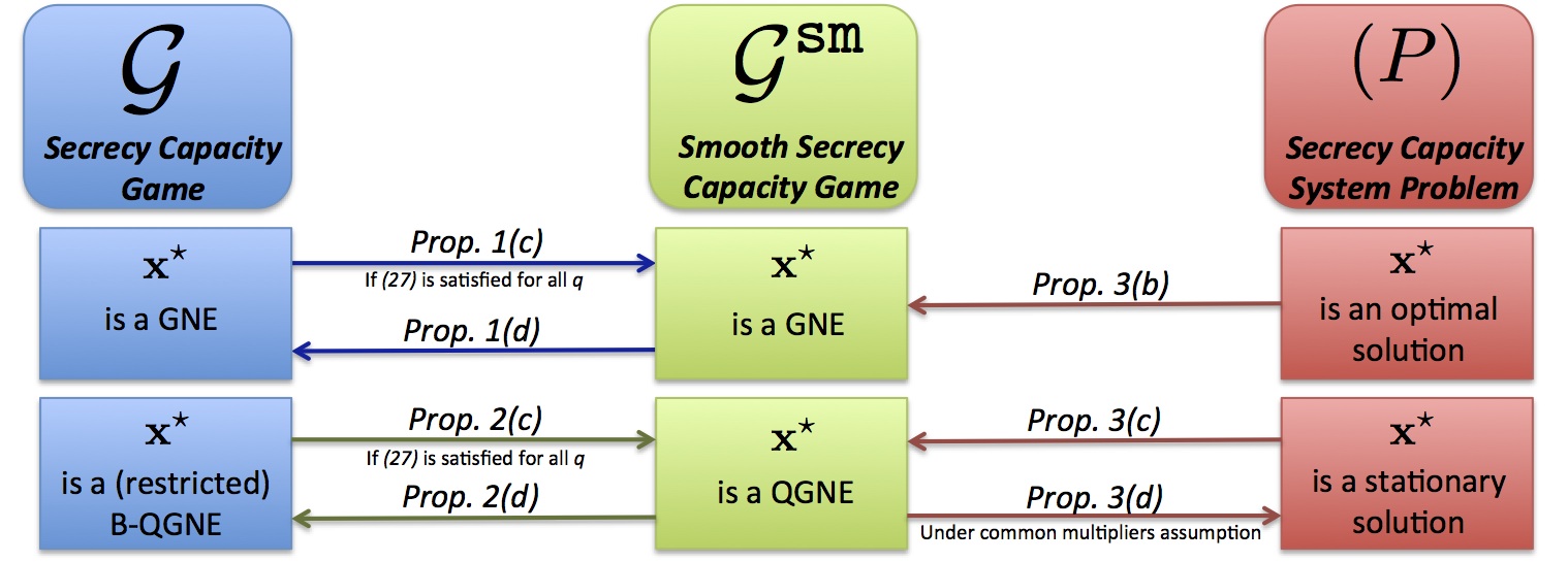
Figure 1: Connections between the games $\mathcal{G}$, $\mathcal{G}^{\texttt{{sm}}}$ and the social problem (P).

Based on Proposition 3, one can now design distributed algorithms for computing a (Q)GNE of $\mathcal{G}^{\texttt{sm}}$ (and thus a restricted B-QGNE of the original game $\mathcal{G}$): it is sufficient to solve the social problem (P). Such a problem is nonconvex; stationary solutions however can be computed efficiently observing that (P) is an instance of the DC program (1), under the following identifications:

$$f_{q}\left(p_{q},{\mathbf{p}}_{q}^{\texttt{{J}}}\right)\triangleq -\log\left(\sigma^{2}+H_{qq}^{\texttt{SD}}p_{q}+{\textstyle\sum_{j=1}^{J}{H}_{jq}^{\texttt{JD}}\,p_{jq}^{\texttt{J}}}\right)$$

$$-\log\left(\sigma^{2}+{\textstyle\sum_{j=1}^{J}{H}_{je}^{\texttt{JE}}\,p_{jq}^{\texttt{J}}}\right)$$

$$g_{q}\left(p_{q},{\mathbf{p}}_{q}^{\texttt{{J}}}\right)\triangleq -\log\left(\sigma^{2}+H_{qe}^{\texttt{SE}}p_{q}+{\textstyle\sum_{j=1}^{J}{H}_{je}^{\texttt{JE}}\,p_{jq}^{\texttt{J}}}\right)$$

$$-\log\left(\sigma^{2}+{\textstyle\sum_{j=1}^{J}{H}_{jq}^{\texttt{JD}}\,p_{jq}^{\texttt{J}}}\right).\vspace{-0.2cm}$$

We can then efficiently compute a stationary solution of (P) using any of the distributed algorithms introduced in Section IV. For instance, Algorithm 1 based on a dual decomposition loop (cf. Algorithm 3) specialized to (P) is given in Algorithm 4, where in (32), $\mathcal{X}_{q}\triangleq\left\{\mathbf{x}_{q}\triangleq(p_{q},\mathbf{p}_{q}^{\texttt{J}})\geq\mathbf{0}\,:\,p_{q}\leq P_{q}\text{ and (\ref{eq:linear_const})}\,\mbox{holds}\right\}$ and $\widetilde{\theta}_{q}(\mathbf{x}_{q};\mathbf{x}_{q}^{\nu})$ is defined as

$$\widetilde{\theta}_{q}(\mathbf{x}_{q};\mathbf{x}_{q}^{\nu})\triangleq f_{q}\left(\mathbf{x}_{q}\right)-\frac{\partial g_{q}(\mathbf{x}_{q}^{\nu})}{\partial p_{q}}\,p_{q}-\sum_{j=1}^{J}\frac{\partial g_{q}(\mathbf{x}_{q}^{\nu})}{\partial p_{jq}^{\texttt{J}}}\,p_{jq}^{\texttt{J}}$$ (31)

$$+\frac{\tau_{q}}{2}\|\mathbf{x}_{q}-\mathbf{x}_{q}^{\nu}\|^{2},$$

with

$$\frac{\partial g_{q}(\mathbf{x}_{q})}{\partial p_{q}} \triangleq-\frac{H_{qe}^{\texttt{SE}}}{\sigma^{2}+H_{qe}^{\texttt{SE}}p_{q}+{\sum_{j=1}^{J}{H}_{je}^{\texttt{JE}}\,p_{jq}^{\texttt{J}}}}$$

$$\frac{\partial g_{q}(\mathbf{x}_{q})}{\partial p_{jq}^{\texttt{J}}} \triangleq-\frac{{H}_{je}^{\texttt{JE}}}{\sigma^{2}+H_{qe}^{\texttt{SE}}p_{q}+{\sum_{j=1}^{J}{H}_{je}^{\texttt{JE}}\,p_{jq}^{\texttt{J}}}}$$

$$\,\,\,\,\,\,\,-\frac{{H}_{jq}^{\texttt{JD}}}{\sigma^{2}+{\sum_{j=1}^{J}{H}_{jq}^{\texttt{JD}}\,p_{jq}^{\texttt{J}}}},\quad j=1,\ldots,J.$$

Data: $\bm{{\tau}}\triangleq(\tau_{q})_{q=1}^{Q}\geq\mathbf{0},\{\gamma^{\nu}\}>0$, $\{\alpha^{t}\}>0$ and $\mathbf{x}^{0}\triangleq\left(\mathbf{p}^{0},{\mathbf{p}}^{\texttt{{J}},0}\right)\in\mathcal{P}$. Set $\nu=0$.

$(\texttt{S.1})$: If $\mathbf{x}^{\nu}\triangleq\left(\mathbf{p}^{\nu},{\mathbf{p}}^{\texttt{{J}},\nu}\right)$ satisfies a termination criterion, STOP;

$(\texttt{S.2a})$: Choose $\bm{\lambda}^{0}\triangleq(\lambda_{j}^{0})_{j=1}^{J}\geq\mathbf{0}$. Set $n=0$.

$(\texttt{S.2b})$: If $\bm{\lambda}^{t}\triangleq(\lambda_{j}^{t})_{j=1}^{J}$ satisfies a termination criterion, set $\widehat{\mathbf{x}}\left(\mathbf{x}^{\nu}\right)=(p_{q}^{t,\,\nu},\mathbf{p}_{q}^{\texttt{J},\,\nu,\,t})_{q=1}^{Q}$ and go to $(\texttt{S.3})$;

$(\texttt{S.2c})$: The legitimate users $q=1,\ldots,Q$ compute in parallel $(p_{q}^{\,\nu,\,t},\mathbf{p}_{q}^{\texttt{J},\,\nu,\,t})$ given by

$$(p_{q}^{\,\nu,\,t},\mathbf{p}_{q}^{\texttt{J},\,\nu,\,t})\triangleq\underset{\mathbf{x}_{q}\triangleq(p_{q},\mathbf{p}_{q}^{\texttt{J}})\in\mathcal{X}_{q}}{\text{argmin}}\,\left\{\widetilde{\theta}_{q}(\mathbf{x}_{q};\mathbf{x}_{q}^{\nu})+\bm{\lambda}^{t}{}^{T}\mathbf{p}_{q}^{\texttt{J}}\right\};$$ (32)

$(\texttt{S.2d})$: Update $\bm{\lambda}\triangleq(\lambda_{j})_{j=1}^{J}$: for all $j=1,\ldots,J$,

$$\lambda_{j}^{t+1}\triangleq\left[0,\lambda_{j}^{t}+\alpha^{t}\left(\sum_{q=1}^{Q}p_{jq}^{\texttt{J},\,\nu,\,t}-P_{j}^{\texttt{J}}\right)\right]_{+};$$ (33)

$(\texttt{S.2e})$: Set $t\leftarrow t+1$ and go back to $(\texttt{S.2b})$;

$(\texttt{S.3})$: Set $\mathbf{x}^{\nu+1}=\mathbf{x}^{\nu}+\gamma^{\nu}\left(\,\widehat{\mathbf{x}}\left(\mathbf{x}^{\nu}\right)-\mathbf{x}^{\nu}\,\right)$;

$(\texttt{S.4})$: $\nu\leftarrow\nu+1$ and go to $(\texttt{S.1})$.

Algorithm 4 : DC-based Algorithm for (P)

If the sequences $\{\gamma^{\nu}\}>0$ and $\{\alpha^{t}\}>0$ are chosen according to one of the rules stated in Theorems 1 and 4, respectively, Algorithm 4 converges to a stationary solution of the social problem (P) (in the sense of Theorem 1), and thus to a QGNE of $\mathcal{G}^{\texttt{{sm}}}$ [cf. Proposition 3c)], which is also a restricted B-QGNE of $\mathcal{G}$ [cf. Proposition 2d)].

Remark 4 (On the implementation of Algorithm 4).

Once the CSI is available at the users’ sides, Algorithm 4 can be implemented in a distributed way, with limited signaling only between the legitimate users and the friendly jammers (no communications among the users or the eavesdropper is required). Indeed, in the inner loop of the algorithm, given the current value of the price $\bm{\lambda}$, all the users simultaneously update the power profiles $(p_{q},\mathbf{p}_{q}^{\texttt{J}})$ solving locally a strongly convex optimization problem. Then, they communicate to the friendly jammers the amount of power they need resulting from the optimization. Given the power requests from the users, the jammers update in parallel and independently their price $\lambda_{j}$ performing an inexpensive scalar projection [cf. (33)], and then broadcast the new price value to the legitimate users. We remark that the proposed scheme require the same CSI and communication overhead than CJ approaches proposed in the literature (see, e.g., [22, 21]).

Remark 5 (More general formulation).

For the sake of simplicity, in the previous sections, we assumed uniform power allocation over the spectrum (still to optimize) from the users and the friendly jammers. We remark however that game $\mathcal{G}$ in (24) [game $\mathcal{G}^{\text{{{sm}}}}$ in (27) and problem (P) in (30)] can be generalized to the case of nonuniform power allocations (over flat-fading channels) and the proposed algorithms extended accordingly. We omit more details because of space limitation.

V-A5 Numerical Results

In this subsection, we present some experiments validating our theoretical findings. We compare our Algorithm 4 with centralized and applicable decentralized schemes existed in the literature (adapted to our formulation).

System setup. All the experiments are obtained in the following setting, unless stated otherwise. All the users and jammers have the same power budget, i.e. $P_{q}=P_{j}^{\texttt{J}}=P$, and we set $\texttt{snr}=P/\sigma^{2}=10$dB. The position of the users, jammers, and eavesdropper are randomly generated within a square area; the channel gains $H_{qq}^{\texttt{SD}}$, $H_{qe}^{\texttt{SE}}$, $H_{jq}^{\texttt{JD}}$ and $H_{je}^{\texttt{JE}}$ are Rayleigh distributed with mean equal to one and normalized by the (square) distance between the transmitter and the receiver; our results are collected only for the channel realizations satisfying condition (26). When present, there are $J=\lfloor Q/2\rfloor$ jammers. Algorithm 4 is initialized by choosing the zero power allocation, and it is terminated when the absolute value of the difference of the System Secrecy Rate (SSR) in two consecutive iterations becomes smaller than $1e$-$5$. Similarly, the inner loop is terminated when the difference of the norm of the prices in two consecutive rounds is less than $1e$-$2$.

Example 1$-$Comparison with decentralized schemes. In Fig. 2(a), we plot the average SSR (taken over 50 independent channel realizations) versus the number $Q$ of legitimate users achieved by our Algorithm 4 (blue-line curves) and by solving the SSR maximization game while assuming i) uniform power allocation for the jammers (black-line curves); or ii) no friendly jammers available (red-line curve). In Fig. 2(b) we plot the average SSR versus the snr for the case of $10$ main users; the rest of the setting is as in Fig. 2(a). The figures show that the proposed approach yields much higher SSR than that achievable by the other schemes, and the gain becomes more significant as the number of users or the snr increases.

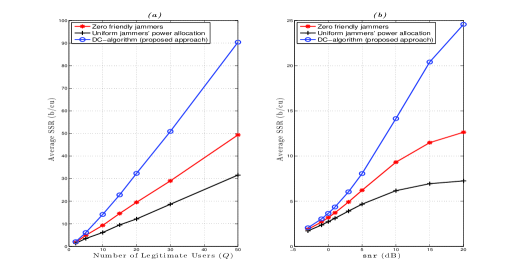
Figure 2: Average system secrecy rate (SSR) versus (a) number $Q$ of legitimate users; (b) snr, for $Q=10$.

Example 2$-$Comparison with centralized schemes. Since Algorithm 4 converges to a stationary solution of the social problem (30), it is natural to compare our scheme with available centralized methods attempting to compute locally or globally optimal solutions (but without rigorously verifying their optimality). More specifically, we consider two schemes: i) the NEOS server [33] based on MINOS solver and PSwarm; and ii) the standard centralized SCA algorithm for DC programs (see, e.g., [13, 12]). Even thought these algorithms are computationally very demanding and not implementable in a distributed network, they represent a good benchmark to test our distributed algorithm. In Fig. 3(a) we plot the probability that the SSR exceeds a given value SSR versus SSR, whereas in Fig. 3(b) we report the average SSR versus the number of legitimate users. All the curves are computed running 100 independent experiments. The figures show that our Algorithm 4 outperforms MINOS, and quite surprisingly it has the same performance of PSwarm and SCA schemes. This means that, at least for the experiments we simulated, Algorithm 4 provides in a distributed way solutions of (30) that are very close to those obtained by centralized methods.

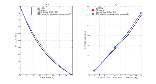
Figure 3: Comparison between our (distributed) Algorithm 4 and centralized approaches.

Example 3$-$Convergence Speed: Table I shows the average number of inner and outer iterations required by Algorithm 4 to converge versus the number of legitimate users, when Rules 1 and 2 [c.f. (12) and (13)] are used for the step-size $\gamma^{\nu}$. The parameters in the two rules are set as $\beta_{1}=1e$-$6$, $\beta_{2}=1e$-$4$, and $\epsilon=1e$-$5$. This average has been taken over 50 independent channel realizations. Notice that, when Rule 2 is used, the number of outer iterations is greatly reduced in comparison to that obtained performing Rule 1. Note also that, the average number of inner iterations per outer iteration is slightly increased in the former case; however, overall, Algorithm 4 with Rule 2 seems to be faster than the same algorithm based on Rule 1. As far as the quality of the achieved SSR is concern, we observed results consistent to Fig. 3.

number of users ($Q$)	2	5	10	15	20	30	50
Rule 1 - outer iterations	46.80	53.62	73.52	95.48	97.74	138.00	175.56
Rule 1 - inner iterations	1.02	1.08	1.19	1.23	1.27	1.23	1.21
Rule 2 - outer iterations	46.66	56.58	66.78	76.12	72.42	83.44	89.56
Rule 2 - inner iterations	1.02	1.08	1.20	1.28	1.30	1.30	1.33

TABLE I: Average number of outer iterations and inner iterations per outer iteration in Algorithm 4 for different choices of diminishing step-size rules.

V-B Case Study #2: Design of CR MIMO systems

V-B1 System model and problem formulation

Consider a hierarchical MIMO CR system composed of $P$ PUs sharing the licensed spectrum with $I$ SUs; the network of SUs is modeled as a $I$-user vector Gaussian interference channel. Each SU $i$ is equipped with $n_{T_{i}}$ and $n_{R_{i}}$ transmit and receive antennas, respectively, and PUs may have multiple antennas. Let $\mathbf{H}_{ji}\!\in\!\mathbb{C}^{n_{R_{j}}\times n_{T_{i}}}$ (resp. $\mathbf{G}_{pi}$) be the cross-channel matrix between the secondary transmitter $i$ and the secondary receiver $j$ (resp. primary receiver $p$). Under basic information theoretical assumptions, the transmission rate of SU $i$ is

$$r_{i}(\mathbf{Q}_{i},\mathbf{Q}_{-i})\triangleq\log\det\left(\mathbf{I}+\mathbf{H}_{ii}^{H}\mathbf{R}_{i}(\mathbf{Q}_{-i})^{-1}\mathbf{H}_{ii}\mathbf{Q}_{i}\right)$$ (34)

where $\mathbf{Q}_{i}$ is the transmit covariance matrix of SU $i$ (to be optimized), $\mathbf{Q}_{-i}\triangleq(\mathbf{Q}_{j})_{j\neq i}$, $\mathbf{R}_{i}(\mathbf{Q}_{-i})\triangleq\mathbf{R}_{n_{i}}+\sum_{j\neq i}\mathbf{H}_{ij}\mathbf{Q}_{j}\mathbf{H}_{ij}^{H}$ with $\mathbf{R}_{n_{i}}\succ\mathbf{0}$ being the covariance matrix of the noise plus the interference generated by the active PUs. Each SU $i$ is subject to the following local constraints

$$\mathcal{Q}_{i}\triangleq\left\{\mathbf{Q}_{i}\succeq\mathbf{0}:\begin{array}[]{l}\mathrm{tr}(\mathbf{Q}_{i})\leq P_{i}^{\mathrm{tot}},\;\mathbf{Q}_{i}\in\mathcal{Z}_{i}\end{array}\right\},$$ (35)

where $P_{i}^{\mathrm{tot}}$ is the total transmit power and $\mathcal{Z}_{i}\subseteq\mathbb{C}^{n_{i}\times n_{i}}$ is an abstract closed and convex set suitable to accommodate (possibly) additional local constraints, such as: i) null constraints $\mathbf{U}_{i}^{H}\mathbf{Q}_{i}=\mathbf{0}$, with $\mathbf{U}_{i}$ being a $n_{T_{i}}\times r_{i}$ (with $r_{i}<n_{T_{i}}$), which prevents SUs to transmit along some prescribed “directions” (the columns of $\mathbf{U}_{i}$); and ii) soft and peak power shaping constraints in the form of $\mathrm{tr}(\mathbf{T}_{i}^{H}\mathbf{Q}_{i}\mathbf{T}_{i})\leq I_{i}^{\text{{ave}}}$ and $\lambda^{\max}(\mathbf{F}_{i}^{H}\mathbf{Q}_{i}\mathbf{F}_{i})\leq I_{i}^{\text{{peak}}}$, which limits to $I_{i}^{\text{{ave}}}>0$ and $I_{i}^{\text{{peak}}}>0$ the total average and peak average power allowed to be radiated along the range space of matrices $\mathbf{T}_{i}\in\mathbb{C}^{n_{T_{i}}\times n_{G_{i}}}$ and $\mathbf{F}_{i}\in\mathbb{C}^{n_{T_{i}}\times n_{F_{i}}}$, respectively. Adopting the spectrum underlay architecture, the interference power at the primary receivers is regulated by imposing global interference constraints to the SUs, in the form of $\sum_{i}\mathrm{tr}(\mathbf{G}_{pi}^{H}\mathbf{Q}_{i}\mathbf{G}_{pi})\leq I_{p}^{\text{{tot}}}$ for all $p=1,\ldots,P,$ where $I_{p}^{\text{{tot}}}>0$ is the interference threshold imposed by PU $p$.

The design of the CR system can be formulated as

$$\!\!\!\!\begin{array}[]{cl}\underset{\mathbf{Q}_{1},\ldots,\mathbf{Q}_{I}}{\textrm{maximize}}&{\theta}(\mathbf{Q})\triangleq\sum_{i=1}^{I}r_{i}(\mathbf{Q}_{i},\mathbf{Q}_{-i})\\ \textrm{subject to}&\mathbf{Q}_{i}\in\mathcal{Q}_{i},\quad i=1,\ldots,I,\vskip 3.0pt plus 1.0pt minus 1.0pt\\ &\sum_{i}\mathrm{tr}(\mathbf{G}_{pi}^{H}\mathbf{Q}_{i}\mathbf{G}_{pi})\leq I_{p}^{\text{{tot}}},\quad p=1,\ldots,P.\end{array}$$ (36)

Special cases of the nonconvex sum-rate maximization problem (36) have already been studied in the literature, e.g., in [7, 28]. However the theoretical convergence of current algorithms is up to date an open problem. Since (36) is an instance of (1), we can capitalize on the framework developed in the first part of the paper and obtain readily a class of distributed algorithms with provable convergence.

V-B2 DC-based decomposition algorithms

We cast first (36) into (1) (in the maximization form). Exploring the DC-structure of the rates $r_{i}(\mathbf{Q}_{i},\mathbf{Q}_{-i})$, the sum-rate ${\theta}(\mathbf{Q})$ can indeed be rewritten as the sum of a concave and convex function, namely: ${\theta}(\mathbf{Q})=\sum_{i}\left(f_{i}(\mathbf{Q})-g_{i}(\mathbf{Q})\right)$, where

$$f_{i}(\mathbf{Q}) \!\!\!\!\triangleq\,\,\,\log\det\left(\mathbf{R}_{n_{i}}+\sum_{j=1}\mathbf{H}_{ij}\mathbf{Q}_{j}\mathbf{H}_{ij}^{H}\right)$$

$$g_{i}(\mathbf{Q}_{-i}) \!\!\!\!\triangleq\,\,\log\det\left(\mathbf{R}_{n_{i}}+\sum_{j\neq i}\mathbf{H}_{ij}\mathbf{Q}_{j}\mathbf{H}_{ij}^{H}\right).$$

We can now use the machinery developed in Sec. III. It is not difficult to show that the approximation function $\widetilde{{\theta}}(\mathbf{x};\mathbf{x}^{\nu})$ in (5) (to be maximized) becomes (up to a constant term) $\widetilde{{\theta}}(\mathbf{Q};\mathbf{Q}^{\nu})\triangleq\sum_{i}\widetilde{{\theta}}_{i}(\mathbf{Q};\mathbf{Q}^{\nu})$, with

$$\!\!\widetilde{{\theta}}_{i}(\mathbf{Q};\mathbf{Q}^{\nu})\!\triangleq\!r_{i}(\mathbf{Q}_{i},\mathbf{Q}_{-i}^{\nu})-\left\langle\mathbf{\Pi}_{i}(\mathbf{Q}^{\nu}),\mathbf{Q}_{i}\!-\!\mathbf{Q}_{i}^{\nu}\right\rangle-\tau_{i}\left\|\mathbf{Q}_{i}-\mathbf{Q}_{i}^{\nu}\right\|_{F}^{2}$$ (37)

where $\mathbf{Q}^{\nu}\triangleq(\mathbf{Q}_{i}^{\nu})_{i=1}^{I}$ with each $\mathbf{Q}_{i}^{\nu}\succeq\mathbf{0}$, $\left\langle\mathbf{A},\mathbf{B}\right\rangle\triangleq\text{{Re}}\left\{\text{{tr}}(\mathbf{A}^{H}\mathbf{B})\right\}$, $\left\|\bullet\right\|_{F}$ is the Frobenius norm, and

$$\mathbf{\Pi}_{i}(\mathbf{Q}^{\nu})\triangleq\sum_{j\in\mathcal{N}_{i}}\,\mathbf{H}_{ji}^{H}\,\widetilde{\mathbf{R}}_{j}(\mathbf{Q}_{-j}^{\nu})\,\mathbf{H}_{ji},\vspace{-0.1cm}$$ (38)

with $\mathcal{N}_{i}$ denoting the set of neighbors of user $i$ (i.e., the set of users $j$’s which user $i$ interferers with), and

$$\widetilde{\mathbf{R}}_{j}(\mathbf{Q}_{-j}^{\nu})\triangleq\mathbf{R}_{j}(\mathbf{Q}_{-j}^{\nu})^{-1}-(\mathbf{R}_{j}(\mathbf{Q}_{-j}^{\nu})+\mathbf{H}_{jj}\mathbf{Q}_{j}^{\nu}\mathbf{H}_{jj}^{H})^{-1}.$$

Therefore a stationary solution of (36) can be efficiently computed using any of the distributed algorithms introduced in Section IV; one just needs to replace $\widetilde{{\theta}}(\mathbf{x};\mathbf{x}^{\nu})$ with $\widetilde{{\theta}}(\mathbf{Q};\mathbf{Q}^{\nu})$ (and the minimization with the maximization). For instance, Algorithm 1 based on a dual decomposition loop (cf. Algorithm 3) can be written in the form of Algorithm 5. Convergence (in the sense of Theorem 1) is guaranteed if the step-size sequences $\{\gamma^{\nu}\}$ and $\{\alpha^{n}\}>0$ are chosen according to one of the rules stated in Theorems 1 and 4, respectively.

Data: $\bm{{\tau}}\triangleq(\tau_{i})_{i=1}^{I}\geq\mathbf{0},\{\gamma^{\nu}\}>0$, $\{\alpha^{t}\}>0$ and $\mathbf{Q}_{i}^{0}\in\mathcal{Q}$ for all $i$. Set $\nu=0$.

$(\texttt{S.1})$: If $\mathbf{Q}^{\nu}\!\!\triangleq\!\!(\mathbf{Q}_{i}^{\nu})_{i=1}^{I}$ satisfies a termination criterion, STOP;

$(\texttt{S.2a})$: Choose $\bm{\lambda}^{0}\triangleq(\lambda_{p}^{0})_{p=1}^{P}\geq\mathbf{0}$. Set $t=0$.

$(\texttt{S.2b})$: If $\bm{\lambda}^{t}\triangleq(\lambda_{p}^{t})_{p=1}^{P}$ satisfies a termination criterion, set $\widehat{\mathbf{Q}}\left(\mathbf{Q}^{\nu}\right)\triangleq(\mathbf{Q}_{i}^{t,\,\nu})_{i=1}^{I}$ and go to $(\texttt{S.3})$;

$(\texttt{S.2c})$: The SUs solve in parallel the following strongly convex optimization problems: for all $i=1,\dots,I$,

$$\mathbf{Q}_{i}^{\,\nu,\,t}\triangleq\underset{\mathbf{Q}_{i}\in\mathcal{Q}_{i}}{\text{argmax}}\left\{\widetilde{\theta}_{i}(\mathbf{Q}_{i};\mathbf{Q}^{\nu})-\sum_{p=1}^{P}\lambda_{p}^{t}\,\mathrm{tr}(\mathbf{G}_{pi}^{H}\mathbf{Q}_{i}\mathbf{G}_{pi})\right\};$$ (39)

$(\texttt{S.2d})$: Update $\bm{\lambda}\triangleq(\lambda_{p})_{p=1}^{P}$: for all $p=1,\ldots,P$,

$$\lambda_{p}^{t+1}\triangleq\left[\lambda_{p}^{t}+\alpha^{t}\left(\sum_{i=1}^{I}\mathrm{tr}(\mathbf{G}_{pi}^{H}\mathbf{Q}_{i}^{\,\nu,\,t}\mathbf{G}_{pi})-I_{p}^{\max}\right)\right]_{+};$$ (40)

$(\texttt{S.2e})$: Set $t\leftarrow t+1$ and go back to $(\texttt{S.2b})$;

$(\texttt{S.3})$: Set $\mathbf{Q}^{\nu+1}=\mathbf{Q}^{\nu}+\gamma^{\nu}\left(\,\widehat{\mathbf{Q}}\left(\mathbf{Q}^{\nu}\right)-\mathbf{Q}^{\nu}\,\right)$;

$(\texttt{S.4})$: $\nu\leftarrow\nu+1$ and go to $(\texttt{S.1})$.

Algorithm 5 : Dual-based Algorithm for (36).

V-B3 Discussion on the implementation of Algorithm 5

The algorithm is a double loop scheme in the sense described next.

Inner loop: In this loop, at every iteration $t$: i) First, all SUs solve in parallel their strongly convex optimization problems (39), for fixed $\bm{{\lambda}}^{t}=(\lambda_{p}^{t})_{p=1}^{P}$, resulting in the optimal solutions $(\mathbf{Q}_{i}^{\,\nu,\,t})_{i=1}^{I}$; ii) Then, given the new interference levels $\sum_{i=1}^{I}\mathrm{tr}(\mathbf{G}_{pi}^{H}\mathbf{Q}_{i}^{\,\nu,\,t}\mathbf{G}_{pi})$, the prices $\bm{{\lambda}}$ are updated in parallel via (40), resulting in $\bm{{\lambda}}^{t+1}=(\lambda_{p}^{t+1})_{p=1}^{P}$. The loop terminates when $\{\bm{\lambda}^{t}\}$ meets the termination criterion in (S.2b).

Outer loop: It consists in updating $\mathbf{Q}_{i}^{\nu}$’s according to (S.3).

Communication overhead: The proposed algorithm is fairly distributed. Indeed, given the interference generated by the other users [the covariance matrix $\mathbf{R}_{i}(\mathbf{Q}_{-i})$, which can be locally measured], and the interference price $\bm{{\Pi}}_{i}(\mathbf{Q}^{\nu})$, each SU can efficiently and locally compute the optimal covariance matrix $\mathbf{Q}_{i}^{\,\nu,\,t}$ by solving (39). Note that, for some specific structures of the feasible sets $\mathcal{Q}_{i}$ and channels (e.g., $\mathcal{Z}_{i}=\emptyset$, full-column rank channel matrices $\mathbf{H}_{ii}$, and $\tau_{i}=0$), a solution of (39) is available in closed form (up to the multipliers associated with the power budget constraints) [7]. The estimation of the prices $\bm{{\Pi}}_{i}(\mathbf{Q}^{\nu})$ requires some signaling exchange but only among nearby users. Interestingly, the pricing expression (38) as well as the signaling overhead necessary to compute it coincides with that of pricing schemes proposed in the literature to solve related problems [7, 10, 8].

The natural candidates for updating the prices in the inner loop are the PUs, after measuring locally the current overall interference $\sum_{i=1}^{I}\mathrm{tr}(\mathbf{G}_{pi}^{H}\mathbf{Q}_{i}^{\,\nu,\,t}\mathbf{G}_{pi})$ from the SUs. Note that this update is computationally inexpensive (it is a projection onto $\mathbb{R}_{+}$), can be performed in parallel among PUs, and does not require any signaling exchange with the SUs. The new value of the prices is then broadcasted to the SUs. In CR scenarios where the PUs cannot participate in the updating process, the SUs themselves can perform the price update, at the cost of more signaling, e.g., using consensus algorithms. Alternatively, if the primary receivers have a fixed geographical location, it might be possible to install some monitoring devices close to each primary receiver having the functionality of price computation and broadcasting.

As a final remark note that, since Algorithm 5 is a dual-base scheme, it is scalable with the number of SUs. However, for the same reasons, there might happen that the interference constraints are not satisfied during the intermediate iterations. This issue can be alleviated in practice by choosing a “large” $\bm{{\lambda}}^{0}$ as initial price. An alternative distributed scheme which does not suffer from this issue can be readily obtained using the primal-based decomposition approach introduced in Sec. IV-B; we omit the details because of space limitation.

VI Conclusions

In this paper we proposed a novel decomposition framework to compute stationary solutions of nonconvex (possibly DC) sum-utility minimization problems with coupling convex constraints. We developed a class of (inexact) best-response-like algorithms, where all the users iteratively solve in parallel a suitably convexified version of the original DC program. To the best of our knowledge, this is the first set of distributed algorithms with provable convergence for multiuser DC programs with coupling constraints. Finally, we tested our methodology on two problems: i) a novel secrecy rate game (for which we provided a nontrivial DC formulation); and ii) the sum-rate maximization problems over CR MIMO networks. Our experiments show that our distributed algorithms reach performance comparable (and sometimes better) than centralized schemes.

Appendix A Proof of Theorem 1

The proof follows from [10, Th.3] and Proposition 4 below, which establishes the main properties of the best-response map $\Xi\ni\mathbf{y}\mapsto\widehat{\mathbf{x}}(\mathbf{y})\in\Xi$ defined in (8), as required by [10, Th.3].

Proposition 4.

Given the DC program (1) under A1-A4, the map $\Xi\ni\mathbf{y}\mapsto\widehat{\mathbf{x}}(\mathbf{y})\in\Xi$ defined in (8) has the following properties:

(a): For every given $\mathbf{y}\in\Xi$, the vector $\widehat{\mathbf{x}}(\mathbf{y})-\mathbf{y}$ is a descent direction of the objective function $\theta(\mathbf{x})$ at $\mathbf{y}$:

$$\left(\widehat{\mathbf{x}}(\mathbf{y})-\mathbf{y}\right)^{T}\nabla_{\mathbf{x}}\theta(\mathbf{y})\leq-c_{\bm{{\tau}}}\,\|\widehat{\mathbf{x}}(\mathbf{y})-\mathbf{y}\|^{2},$$ (41)

with $c_{\bm{\tau}}$ defined in (10);

(b): $\widehat{\mathbf{x}}(\bullet)$ is Lipschitz continuos on $\Xi$, with constant $L_{\widehat{\mathbf{x}}}\triangleq L_{\nabla\widetilde{\theta}}/c_{\bm{\tau}}$, where $L_{\nabla\widetilde{\theta}}$ is defined in Lemma 3 below;

(c): The set of fixed points of $\widehat{\mathbf{x}}(\bullet)$ coincides with the set of stationary points of the optimization problem (1); therefore $\widehat{\mathbf{x}}(\bullet)$ has a fixed point.

Proof. Before proving the proposition, we introduce the following lemma, whose proof is omitted (see attached material).

Lemma 3.

In the setting of Proposition 4, $\nabla\widetilde{\theta}({\mathbf{x}};\bullet)$ is uniformly Lipschitz on $\Xi$, that is, for any given $\mathbf{x}\in\Xi$,

$$\left\|\nabla_{\mathbf{x}}\widetilde{\theta}({\mathbf{x}};\mathbf{y})-\nabla_{\mathbf{x}}\widetilde{\theta}({\mathbf{x}};\mathbf{z})\right\|\leq L_{\nabla\widetilde{\theta}}\,\left\|\mathbf{z}-\mathbf{y}\right\|,\quad\forall\mathbf{y},\mathbf{z}\in\Xi,$$ (42)

with $L_{\nabla\widetilde{\theta}}^{2}\triangleq 4\,(L_{\nabla\theta}^{2}+2\sum_{i=1}^{I}L_{\nabla f_{i}}^{2}+\tau^{\max})$, where $L_{\nabla\theta}$ and $L_{\nabla f_{i}}$ are defined in assumption A3, and $\tau^{\max}\triangleq\max_{i}\tau_{i}^{2}$.

We prove next only (a) and (b) of Proposition 4.

(a): Given $\mathbf{y}\in\Xi$, by definition, $\widehat{\mathbf{x}}(\mathbf{y})$ satisfies the minimum principle associated with (8): for all $\mathbf{z}\triangleq\left(\mathbf{z}_{i}\right)_{i=1}^{I}\in\Xi$,

$$\left(\mathbf{z}-\widehat{\mathbf{x}}(\mathbf{y})\right)^{T}\nabla_{\mathbf{x}}\widetilde{\theta}(\widehat{\mathbf{x}}(\mathbf{y});\mathbf{y})\geq 0$$ (43)

$$\sum_{i=1}^{I}\left(\mathbf{z}_{i}-\widehat{\mathbf{x}}_{i}(\mathbf{y})\right)^{T}\left[\nabla_{\mathbf{x}_{i}}f_{i}(\widehat{\mathbf{x}}_{i}(\mathbf{y}),\mathbf{y}_{-i})+\sum_{j\neq i}\nabla_{\mathbf{x}_{i}}f_{j}(\mathbf{y})\right.$$

$$\left.-\sum_{j=1}^{I}\nabla_{\mathbf{x}_{i}}g_{j}(\mathbf{y})+\tau_{i}\left(\widehat{\mathbf{x}}_{i}(\mathbf{y})-\mathbf{y}_{i}\right)\right]\geq 0.$$

Letting $\mathbf{z}_{i}=\mathbf{y}_{i}$, and, adding and subtracting $\nabla_{\mathbf{x}_{i}}f_{i}(\mathbf{y})$ in each term $i$ of the sum in (43), we obtain:

$$\left(\mathbf{y}-\widehat{\mathbf{x}}(\mathbf{y})\right)^{T}\nabla_{\mathbf{x}}\theta(\mathbf{y})$$ (44)

$$\geq\sum_{i=1}^{I}\left(\widehat{\mathbf{x}}_{i}(\mathbf{y})-\mathbf{y}_{i}\right)^{T}\left(\nabla_{\mathbf{x}_{i}}f_{i}(\widehat{\mathbf{x}}_{i}(\mathbf{y}),\mathbf{y}_{-i})-\nabla_{\mathbf{x}_{i}}f_{i}(\mathbf{y})\right)$$

$$\,\,\,\,\,\,\,+\sum_{i=1}^{N}\tau_{i}\|\widehat{\mathbf{x}}_{i}(\mathbf{y})-\mathbf{y}_{i}\|^{2}\geq c_{\bm{{\tau}}}\,\|\widehat{\mathbf{x}}(\mathbf{y})-\mathbf{y}\|^{2},\vspace{0.2cm}$$

where in the last inequality we used the definition of $c_{\bm{\tau}}$. This completes the proof of (a).

(b): Let $\mathbf{y},\mathbf{z}\in\Xi$; by the minimum principle, we have

$$\left(\mathbf{v}-\widehat{\mathbf{x}}(\mathbf{y})\right)^{T}\nabla_{{\mathbf{x}}}\widetilde{\theta}(\widehat{\mathbf{x}}(\mathbf{y});\mathbf{y}) \geq 0\qquad\forall\mathbf{v}\in\Xi$$

$$\left(\mathbf{w}-\widehat{\mathbf{x}}(\mathbf{z})\right)^{T}\nabla_{{\mathbf{x}}}\widetilde{\theta}(\widehat{\mathbf{x}}(\mathbf{z});\mathbf{z}) \geq 0\qquad\forall\mathbf{w}\in\Xi.$$ (45)

Setting $\mathbf{v}=\widehat{\mathbf{x}}(\mathbf{z})$ and $\mathbf{w}=\widehat{\mathbf{x}}(\mathbf{y})$ and summing the two inequalities above, after some manipulations, we obtain:

$$\begin{array}[]{l}\left(\widehat{\mathbf{x}}(\mathbf{z})-\widehat{\mathbf{x}}(\mathbf{y})\right)^{T}\left(\nabla_{{\mathbf{x}}}\widetilde{\theta}(\widehat{\mathbf{x}}(\mathbf{z});\mathbf{z})-\nabla_{{\mathbf{x}}}\widetilde{\theta}(\widehat{\mathbf{x}}(\mathbf{y});\mathbf{z})\right)\\ \leq\left(\widehat{\mathbf{x}}(\mathbf{y})-\widehat{\mathbf{x}}(\mathbf{z})\right)^{{T}}\left(\nabla_{{\mathbf{x}}}\widetilde{\theta}(\widehat{\mathbf{x}}(\mathbf{y});\mathbf{z})-\nabla_{{\mathbf{x}}}\widetilde{\theta}(\widehat{\mathbf{x}}(\mathbf{y});\mathbf{y})\right).\end{array}$$ (46)

The Lipschitz property of $\widehat{\mathbf{x}}(\bullet)$, as stated in Proposition 4(b), comes from (46) using the following lower and upper bounds:

$$\begin{array}[]{l}\left(\widehat{\mathbf{x}}(\mathbf{z})-\widehat{\mathbf{x}}(\mathbf{y})\right)^{{T}}\left(\nabla_{{\mathbf{x}}}\widetilde{\theta}(\widehat{\mathbf{x}}(\mathbf{z});\mathbf{z})-\nabla_{{\mathbf{x}}}\widetilde{\theta}(\widehat{\mathbf{x}}(\mathbf{y});\mathbf{y})\right)\\ \geq c_{{\bm{\tau}}}\left\|\widehat{\mathbf{x}}(\mathbf{z})-\widehat{\mathbf{x}}(\mathbf{y})\right\|^{{2}}\vspace{-0.1cm}\end{array}$$ (47)

and

$$\begin{array}[]{l}\left(\widehat{\mathbf{x}}(\mathbf{y})-\widehat{\mathbf{x}}(\mathbf{z})\right)^{{T}}\left(\nabla_{{\mathbf{x}}}\widetilde{\theta}(\widehat{\mathbf{x}}(\mathbf{y});\mathbf{z})-\nabla_{{\mathbf{x}}}\widetilde{\theta}(\widehat{\mathbf{x}}(\mathbf{y});\mathbf{y})\right)\\ \leq\,L_{\nabla\widetilde{\theta}}\,\left\|\widehat{\mathbf{x}}(\mathbf{y})-\widehat{\mathbf{x}}(\mathbf{z})\right\|\,\left\|\mathbf{z}-\mathbf{y}\right\|\end{array}$$ (48)

where (47) is a direct consequence of the uniform strong convexity of $\widetilde{\theta}$, whereas (48) follows from the Cauchy-Schwartz inequality and Lemma 3. Combining (46), (47), and (48), we obtain the desired result.

Appendix B Proof of Proposition 1

(a) It is not difficult to check that $\mathcal{G}$ is an exact potential game with potential function $\Phi(\mathbf{p},\mathbf{p}^{\texttt{{J}}})\triangleq\sum_{q}r_{q}^{s}(p_{q},\mathbf{p}_{q}^{\texttt{{J}}})$. It turns out that any optimal solution of the associated multiplayer maximization problem:

$$\begin{array}[]{ll}\underset{\left(\mathbf{p},{\mathbf{p}}^{\texttt{{J}}}\right)\geq\mathbf{0}}{\text{maximize}}&\Phi(\mathbf{p},\mathbf{p}^{\texttt{{J}}})\\ \text{subject to:}&\begin{array}[t]{c}\vspace{-0.4cm}\hfil\\ \begin{array}[t]{l}\begin{array}[]{ll}p_{q}\leq P_{q},&\forall q=1,\ldots,Q\\ {\displaystyle{\sum_{r=1}^{Q}}}\>p_{jr}^{\texttt{{J}}}\leq P_{j}^{\texttt{{J}}},&\forall\,j=1,\ldots,J,\end{array}\end{array}\end{array}\end{array}$$ (49)

is a GNE of $\mathcal{G}$. Since (49) has a solution, there must exist a GNE for $\mathcal{G}$.

(b) The proof is based on similar arguments as those in (a).

(c) Suppose that $\mathbf{x}^{\star}\triangleq\left(\mathbf{p}_{q}^{\star},\mathbf{p}_{q}^{\texttt{J}\star}\right)_{q=1}^{Q}$ is a GNE of $\mathcal{G}$ satisfying (26) for all $q=1,\ldots,Q$. Then, for every $q$, we have: $\left(\mathbf{p}_{q}^{\star},\mathbf{p}_{q}^{\texttt{J}\star}\right)\in\mathcal{P}_{q}^{\texttt{sm}}(\mathbf{p}_{-q}^{\texttt{J}\star})$ and

$$\widetilde{r_{q}^{s}}\left(\mathbf{p}_{q}^{\star},\mathbf{p}_{q}^{\texttt{J}\star}\right)=r_{q}^{s}\left(\mathbf{p}_{q}^{\star},\mathbf{p}_{q}^{\texttt{J}\star}\right)\geq r_{q}^{s}\left(\mathbf{p}_{q},\mathbf{p}_{q}^{\texttt{J}}\right)=\widetilde{r_{q}^{s}}\left(\mathbf{p}_{q},\mathbf{p}_{q}^{\texttt{J}}\right),$$

for all $\left(\mathbf{p}_{q},\mathbf{p}_{q}^{\texttt{J}}\right)\in\mathcal{P}_{q}^{\texttt{sm}}(\mathbf{p}_{-q}^{\texttt{J}\star})$. Therefore, $\left(\mathbf{p}_{q}^{\star},\mathbf{p}_{q}^{\texttt{J}\star}\right)$ is a solution of (27), with $\mathbf{p}_{-q}^{\texttt{J}}=\mathbf{p}_{-q}^{\texttt{J}\star}$.

(d) Suppose that $\mathbf{x}^{\star}\triangleq\left(\mathbf{p}_{q}^{\star},\mathbf{p}_{q}^{\texttt{J}\star}\right)_{q=1}^{Q}$ is a GNE of $\mathcal{G}^{\texttt{sm}}$. Then, for each $q$, $\left(\mathbf{p}_{q}^{\star},\mathbf{p}_{q}^{\texttt{J}\star}\right)\in\mathcal{P}_{q}(\mathbf{p}_{-q}^{\texttt{J}\star})$ and

$$r_{q}^{s}\left(\mathbf{p}_{q}^{\star},\mathbf{p}_{q}^{\texttt{J}\star}\right)=\widetilde{r_{q}^{s}}\left(\mathbf{p}_{q}^{\star},\mathbf{p}_{q}^{\texttt{J}\star}\right)\geq\widetilde{r_{q}^{s}}\left(\mathbf{p}_{q},\mathbf{p}_{q}^{\texttt{J}}\right)=r_{q}^{s}\left(\mathbf{p}_{q},\mathbf{p}_{q}^{\texttt{J}}\right),$$

for all $\left(\mathbf{p}_{q},\mathbf{p}_{q}^{\texttt{J}}\right)\in\mathcal{P}_{q}^{\texttt{sm}}(\mathbf{p}_{-q}^{\texttt{J}\star})$. Since $r_{q}^{s}\left(\mathbf{p}_{q},\mathbf{p}_{q}^{\texttt{J}}\right)=0$ for all $\left(\mathbf{p}_{q},\mathbf{p}_{q}^{\texttt{J}}\right)\in\mathcal{P}_{q}(\mathbf{p}_{-q}^{\texttt{J}\star})\setminus\mathcal{P}_{q}^{\texttt{sm}}(\mathbf{p}_{-q}^{\texttt{J}\star})$ , we have

$$r_{q}^{s}\left(\mathbf{p}_{q}^{\star},\mathbf{p}_{q}^{\texttt{J}\star}\right)\geq r_{q}^{s}\left(\mathbf{p}_{q},\mathbf{p}_{q}^{\texttt{J}}\right),\quad\forall\left(\mathbf{p}_{q},\mathbf{p}_{q}^{\texttt{J}}\right)\in\mathcal{P}_{q}(\mathbf{p}_{-q}^{\texttt{J}\star}).$$

Therefore, $\left(\mathbf{p}_{q}^{\star},\mathbf{p}_{q}^{\texttt{J}\star}\right)$ is a solution of (24), with $\mathbf{p}_{-q}^{\texttt{J}}=\mathbf{p}_{-q}^{\texttt{J}\star}$.

Appendix C Proof of Proposition 2

(a) It follows from Proposition 1(a) that a GNE of $\mathcal{G}$ always exists; since the players’ optimization problems in $\mathcal{G}$ have polyhedral sets, every GNE of $\mathcal{G}$ is also a B-QGNE. Therefore a B-QGNE of $\mathcal{G}$ exists.

(b) It follows from Proposition 1(b) and similar arguments as in the proof of (a).

(c) This proof is based on the following fact, regarding the directional derivative of the plus function [34, Eq. 2.124]:

$$r_{q}^{s}{{}^{\prime}}(\mathbf{z};\mathbf{y}-\mathbf{z}) =[\max(0,\widetilde{r_{q}^{s}}(\bullet))]{{}^{\prime}}(\mathbf{z};\mathbf{y}-\mathbf{z})$$ (50)

$$=\left\{\begin{array}[]{lc}\max\left(0,\nabla_{\mathbf{x}_{q}}\widetilde{r_{q}^{s}}(\mathbf{z})^{T}(\mathbf{y}-\mathbf{z})\right),&\text{if }\widetilde{r_{q}^{s}}(\mathbf{z})=0\vspace{0.05in}\\ \nabla_{\mathbf{x}_{q}}\widetilde{r_{q}^{s}}(\mathbf{z})^{T}(\mathbf{y}-\mathbf{z}),&\text{if }\widetilde{r_{q}^{s}}(\mathbf{z})>0.\end{array}\right.$$

Let $\mathbf{x}^{\star}\triangleq\left(\mathbf{x}_{q}^{\star}\right)_{q=1}^{Q}$ be a (restricted) B-QGNE of $\mathcal{G}$ satisfying (26) for all $q=1,\ldots,Q$, with $\mathbf{x}_{q}^{\star}\triangleq\left(\mathbf{p}_{q}^{\star},\mathbf{p}_{q}^{\texttt{J}\star}\right)$. Then, for every $q$, based on (50), consider the following two cases:

Case I: $\widetilde{r_{q}^{s}}(\mathbf{x}_{q}^{\star})>0$. For all $\mathbf{x}_{q}\in\mathcal{P}_{q}^{\texttt{sm}}(\mathbf{p}_{-q}^{\texttt{J}\star})$ we have

$$0\geq r_{q}^{s}{{}^{\prime}}(\mathbf{x}_{q}^{\star};\mathbf{x}_{q}-\mathbf{x}_{q}^{\star})=\nabla_{\mathbf{x}_{q}}\widetilde{r_{q}^{s}}(\mathbf{x}_{q}^{\star})^{T}\left(\mathbf{x}_{q}-\mathbf{x}_{q}^{\star}\right).$$

Case II: $\widetilde{r_{q}^{s}}(\mathbf{x}_{q}^{\star})=0$. For all $\mathbf{x}_{q}\in\mathcal{P}_{q}^{\texttt{sm}}(\mathbf{p}_{-q}^{\texttt{J}\star})$ we have

$$0\geq r_{q}^{s}{{}^{\prime}}(\mathbf{x}_{q}^{\star};\mathbf{x}_{q}-\mathbf{x}_{q}^{\star})\geq\nabla_{\mathbf{x}_{q}}\widetilde{r_{q}^{s}}(\mathbf{x}_{q}^{\star})^{T}\left(\mathbf{x}_{q}-\mathbf{x}_{q}^{\star}\right).$$

The desired result follows readily from the above two cases.

(d) Let $\mathbf{x}^{\star}\triangleq\left(\mathbf{x}_{q}^{\star}\right)_{q=1}^{Q}$ be a QGNE of $\mathcal{G}^{\texttt{sm}}$, with $\mathbf{x}_{q}^{\star}\triangleq\left(\mathbf{p}_{q}^{\star},\mathbf{p}_{q}^{\texttt{J}\star}\right)$. Consider an arbitrary $q$. Then $\mathbf{x}_{q}^{\star}\in\mathcal{P}_{q}(\mathbf{p}_{-q}^{\texttt{J}\star})$. Based on (50), consider the following two cases:

Case I: $\widetilde{r_{q}^{s}}(\mathbf{x}_{q}^{\star})>0$. For all $\mathbf{x}_{q}\in\mathcal{P}_{q}^{\texttt{sm}}(\mathbf{p}_{-q}^{\texttt{J}\star})$ we have

$$r_{q}^{s}{{}^{\prime}}(\mathbf{x}_{q}^{\star};\mathbf{x}_{q}-\mathbf{x}_{q}^{\star})=\nabla_{\mathbf{x}_{q}}\widetilde{r_{q}^{s}}(\mathbf{x}_{q}^{\star})^{T}\left(\mathbf{x}_{q}-\mathbf{x}_{q}^{\star}\right)\leq 0$$

Case II: $\widetilde{r_{q}^{s}}(\mathbf{x}_{q}^{\star})=0$. For all $\mathbf{x}_{q}\in\mathcal{P}_{q}^{\texttt{sm}}(\mathbf{p}_{-q}^{\texttt{J}\star})$ we have

$$r_{q}^{s}{{}^{\prime}}(\mathbf{x}_{q}^{\star};\mathbf{x}_{q}-\mathbf{x}_{q}^{\star})=\max\left(0,\nabla_{\mathbf{x}_{q}}\widetilde{r_{q}^{s}}(\mathbf{x}_{q}^{\star})^{T}\left(\mathbf{x}_{q}-\mathbf{x}_{q}^{\star}\right)\right)=0$$

The desired result comes readily from the above two cases.

References

- [1] K. Phan, S. Vorobyov, C. Telambura, and T. Le-Ngoc, “Power control for wireless cellular systems via D.C. programming,” in IEEE/SP 14th Workshop on Statistical Signal Processing, 2007, pp. 507–511.
- [2] H. Al-Shatri and T. Weber, “Achieving the maximum sum rate using D.C. programming in cellular networks,” IEEE Trans. Signal Process., vol. 60, no. 3, pp. 1331–1341, March 2012.
- [3] N. Vucic, S. Shi, and M. Schubert, “DC programming approach for resource allocation in wireless networks,” in 8th International Symposium on Modeling and Optimization in Mobile, Ad Hoc and Wireless Networks (WiOpt), 2010, pp. 380–386.
- [4] A. Khabbazibasmenj, F. Roemer, S. Vorobyov, and M. Haardt, “Sum-rate maximization in two-way AF MIMO relaying: Polynomial time solutions to a class of DC programming problems,” IEEE Trans. Signal Process., vol. 60, no. 10, pp. 5478–5493, 2012.
- [5] Y. Xu, T. Le-Ngoc, and S. Panigrahi, “Global concave minimization for optimal spectrum balancing in multi-user DSL networks,” IEEE Trans. Signal Process., vol. 56, no. 7, pp. 2875–2885, July 2008.
- [6] P. Tsiaflakis, M. Diehl, and M. Moonen, “Distributed spectrum management algorithms for multiuser dsl networks,” vol. 56, no. 10, pp. 4825–4843, Oct. 2008.
- [7] S.-J. Kim and G. B. Giannakis, “Optimal resource allocation for MIMO ad hoc cognitive radio networks,” IEEE Trans. Inf. Theory, vol. 57, no. 5, pp. 3117–3131, May 2011.
- [8] D. Schmidt, C. Shi, R. Berry, M. Honig, and W. Utschick, “Distributed resource allocation schemes: Pricing algorithms for power control and beamformer design in interference networks,” IEEE Signal Processing Magazine, vol. 26, no. 5, pp. 53–63, Sept. 2009.
- [9] M. Hong and Z.-Q. Luo, “Signal processing and optimal resource allocation for the interference channel,” Elsevier e-Reference-Signal Processing, 2013. Available at http://arxiv.org/pdf/1206.5144v1.pdf.
- [10] G. Scutari, F. Facchinei, P. Song, D. Palomar, and J. Pang, “Decomposition by partial linearization: Parallel optimization of multi-agent systems,” IEEE Trans. Signal Process., (submitted, Jan. 2013). [Online]. Available: http://arxiv.org/pdf/1302.0756v1.pdf
- [11] R. Horst and N. V. Thoai, “DC programming: overview,” J. Optim. Theory Appl., vol. 103, no. 1, pp. 1–43, Oct. 1999.
- [12] M. Razaviyayn, M. Hong, and Z.-Q. Luo, “A unified convergence analysis of block successive minimization methods for nonsmooth optimization,” Arxiv.org, Oct. 2012. [Online]. Available: http://arxiv.org/abs/1209.2385
- [13] L. An and T. Pham Dinh, “The DC (difference of convex functions) programming and DCA revisited with DC models of real world nonconvex optimization problems,” Annals of Operations Research, vol. 133, no. 1-4, pp. 23–46, 2005.
- [14] D. P. Bertsekas and J. N. Tsitsiklis, Parallel and distributed computation: numerical methods, 2nd ed. Athena Scientific Press, 1989.
- [15] D. Palomar and M. Chiang, “Alternative distributed algorithms for network utility maximization: Framework and applications,” IEEE Trans. Autom. Control, vol. 52, no. 12, pp. 2254–2269, Dec. 2007.
- [16] E. Jorswieck, A. Wolf, and S. Gerbracht, Secrecy on the Physical Layer in Wireless Networks. INTECH, 2010, ch. 20, pp. 413–435.
- [17] L. Dong, Z. Han, A. Petropulu, and H. Poor, “Improving wireless physical layer security via cooperating relays,” IEEE Trans. Signal Process., vol. 58, no. 3, pp. 1875–1888, March 2010.
- [18] X. He and A. Yener, “Cooperative jamming: The tale of friendly interference for secrecy,” in Securing Wireless Communications at the Physical Layer. Springer, 2010, pp. 65–88.
- [19] J. Li, A. Petropulu, and S. Weber, “On cooperative relaying schemes for wireless physical layer security,” IEEE Trans. Signal Process., vol. 59, no. 10, pp. 4985–4997, Oct. 2011.
- [20] Y. Wu and K. J. R. Liu, “An information secrecy game in cognitive radio networks,” IEEE Trans. Inf. Forensics Security, vol. 6, no. 3, pp. 831–842, Sept. 2011.
- [21] I. Stanojev and A. Yener, “Improving secrecy rate via spectrum leasing for friendly jamming,” IEEE Trans. Wireless Commun., vol. 12, no. 1, pp. 134–145, Jan. 2013.
- [22] Z. Han, N. Marina, M. Debbah, and A. Hjørungnes, “Physical layer security game: interaction between source, eavesdropper, and friendly jammer,” EURASIP J. Wireless Commun. Netw., vol. 2009, pp. 11:1–11:10, March 2009.
- [23] Y. Yang, Q. Li, W.-K. Ma, J. Ge, and P. Ching, “Cooperative secure beamforming for AF relay networks with multiple eavesdroppers,” IEEE Signal Process. Lett., vol. 20, no. 1, pp. 35–37, Jan. 2013.
- [24] Q. Li, M. Hong, H.-T. Wai, Y.-F. Liu, W.-K. Ma, and Z.-Q. Luo, “Transmit solutions for MIMO wiretap channels using alternating optimization,” IEEE J. on Selec. Areas in Comm., vol. 31, no. 9, pp. 1714–1727, Sept. 2013.
- [25] J. Pang and G. Scutari, “Nonconvex games with side constraints,” SIAM J. on Optimization, vol. 21, no. 4, pp. 1491–1522, Dec. 2011.
- [26] J.-S. Pang and G. Scutari, “Joint sensing and power allocation in nonconvex cognitive radio games: Quasi-nash equilibria,” IEEE Trans. Signal Process., vol. 61, no. 9, pp. 2366–2382, May 2013.
- [27] R. Zhang, Y.-C. Liang, and S. Cui, “Dynamic resource allocation in cognitive radio networks,” IEEE Signal Processing Magazine, vol. 27, no. 3, pp. 102–114, 2010.
- [28] Y. Zhang, E. Dall’Anese, and G. B. Giannakis, “Distributed optimal beamformers for cognitive radios robust to channel uncertainties,” IEEE Trans. Signal Process., vol. 60, no. 12, pp. 6495–6508, Dec. 2012.
- [29] F. Facchinei and J.-S. Pang, Finite-Dimensional Variational Inequalities and Complementarity Problem. Springer-Verlag, New York, 2003.
- [30] D. P. Bertsekas, A. Nedić, and A. E. Ozdaglar, Convex analysis and optimization. Athena Scientific Belmont, 2003.
- [31] Y. Nesterov, Introductory Lectures on Convex Optimization: A Basic Course (Applied Optimization). Springer, 2004.
- [32] F. Facchinei and C. Kanzow, “Generalized nash equilibrium problems,” A Quart. J. Operat. Res. (4OR), vol. 5, no. 3, pp. 173–210, Sept. 2007.
- [33] J. Czyzyk, M. P. Mesnier, and J. J. Moré, “The NEOS server,” IEEE Comput. Sci. Eng., vol. 5, no. 3, pp. 68–75, Jul-Sep 1998.
- [34] J. F. Bonnans and A. Shapiro, Perturbation analysis of optimization problems. Springer Verlag, 2000.