Evidence of Increased UV Fe ii Emission in Quasars in Candidate Overdense Regions

Abstract

We present evidence for a skewed distribution of UV Fe ii emission in quasars within candidate overdense regions spanning spatial scales of $\sim 50$ Mpc at $1.11<z<1.67$, compared to quasars in field environments at comparable redshifts. The overdense regions have an excess of high equivalent width sources (W2400 $>$ 42 Å), and a dearth of low equivalent width sources. There are various possible explanations for this effect, including dust, Ly$\alpha$ fluorescence, microturbulence, and iron abundance. We find that the most plausible of these is enhanced iron abundance in the overdense regions, consistent with an enhanced star formation rate in the overdense regions compared to the field.

1 INTRODUCTION

There is significant controversy over the stellar mass-metallicity (M-Z) relation as a function of environment and redshift. The general expectation might be that metallicity is higher in overdense regions at a given redshift, since high redshift starburst galaxies seem to prefer such regions (Gómez et al., 2003; Blain et al., 2004; Farrah et al., 2006; Cooper et al., 2008). Earlier star formation would give rise to earlier metal enrichment of the ISM/IGM. For example, supernovae (e.g. Adelberger et al., 2005; Domainko et al., 2004) may efficiently enrich the IGM over Mpc scales.

Conversely, direct observational studies are ambiguous. At low redshift, some authors (e.g. Hughes et al., 2013) find no relation between metallicity and environment, while others (Skillman et al., 1996; Cooper et al., 2008) claim a weak but significant trend for galaxies in groups or clusters to have higher metallicities than field galaxies. At higher redshifts, there is even more uncertainty (e.g. Hamann & Ferland, 1993) with few studies considering environment.

A potentially powerful way to constrain star formation histories in different environments at high redshifts is to use the ratio of Fe  ii[UV] to Mg ii[$\lambda$2798]. To first order, Fe  ii is produced from SNeIa roughly one Gyr after the initial burst of star formation, while Mg ii is created in SNeII. Hence their ratio can be used as a cosmological clock (Hamann & Ferland, 1993) to age-date the initial star formation. Moreover, both emission lines are seen in quasars, where the quasar illuminates the metal rich gas. This allows the lines and therefore the metallicities to be observed to potentially very high redshifts. However there is a large amount of scatter seen in this ratio, the reasons for which are not fully understood.

UV Fe ii has been observed in different objects such as symbiotic stars (e.g Hartman & Johansson, 2000), young stellar objects (e.g. Cooper et al., 2013), novae (e.g Johansson & Jordan, 1984) and the Broad Line Region (BLR) of active galactic nuclei (AGN) (Sigut & Pradhan, 1998). In AGN, UV Fe ii is seen at varying strengths, though the reasons for this variation are still debated. A number of Fe ii-bright quasars have been found and studied in detail over a wide redshift range (e.g. Osterbrock, 1976; Weymann et al., 1991; Graham et al., 1996; Vestergaard & Wilkes, 2001; Bruhweiler & Verner, 2008).

While several mechanisms likely affect the observed iron emission (e.g. abundance, collisional excitation, microturbulence and Ly$\alpha$ fluorescence, see e.g. Netzer & Wills 1983; Sigut & Pradhan 2003; Baldwin et al. 2004; Matsuoka et al. 2007), it is plausible (given that all but abundance are small $<$pc scale mechanisms and unlikely to be effected by the $>$Mpc scale environment) that this emission is a reasonably proxy for the metallicity build up in galaxies.

In this paper, we explore the use of the UV Fe ii in high redshift quasar spectra to consider differences in SFHs in different environments at high redshift. To do so, we consider the overdense regions of quasars in Large Quasar Groups (LQGs).

LQGs are some of the largest candidate overdensities seen in the Universe, spanning 50-200 $h^{-1}$ Mpc, have been found at $z>1$, and are potentially the precursors of the large overdensities seen at the present epoch, such as super-clusters (Komberg, Kravtsov & Lukash, 1996; Wray et al., 2006). These LQGs exist at high redshifts and presumably trace the mass distribution. There are $\sim$ 40 published examples of LQGs (Clowes et al., 2012, (CCGS12) and references therein).

By using LQGs we can quickly assemble statistically significant numbers of quasars in overdense regions, to compare to field samples. The observations for this paper were taken in the direction of the Clowes-Campusano LQG (CCLQG; Clowes & Campusano 1991, 1994) which lies at a redshift of $z\sim 1.3$, and spans $\sim$100-200 $h^{-1}$ Mpc.

We compare the UV Fe ii in quasars in LQGs at $z>1$ to the same emission seen in quasars in the field over similar redshifts to search for differences in star formation history as a function of environment. We will present 12 AGN at $z$ = [1.159,1.689] with increased UV Fe ii emission (W2400 $>$ 32Å) evident in their spectra. All of the quasars are within an area of 1.6 deg², and lie within the redshift range of the overdensity previously described. The cosmology used is $H_{0}=70$ kms^-1Mpc^-1, $\Omega_{m}=0.27$ and $\Omega_{\Lambda}=0.73$.

2 ANALYSIS

We treat the LQG region as a potential high density environment.

By comparing the measurements of the Fe ii emission in these quasars to the emission from a control sample of randomly selected quasars, we examine any differences between the samples. Due to the limits of the observations, we do not study the whole LQGs field, using only two 0.8 deg² of the area (which is covered by our additional observations described later in this section). These fields are centred on RA = 162.146, Dec = 5.406, and RA = 162.514, Dec = 4.528.

2.1 FE ii MEASUREMENT TECHNIQUES

To measure the Fe ii emission, we used the method described in Weymann et al. (1991). We use this method to provide an estimate of the overall emission as opposed to, for example, the Hartig & Baldwin (1986) method which gives an estimate at a single wavelength. The continuum level is found at the central wavelength within two wavelength ranges, 2240–2255 Å and 2665–2695 Å. A straight line is then drawn between the centres of these two wavelength ranges to create the effective continuum. Weymann et al. (1991) calculate the equivalent width (EW) between 2255 and 2650 Å (W2400) with respect to this effective continuum level. The errors on the measurements are estimated based on the noise across the continuum which has the greatest effect and therefore the dominant error in the Fe ii measurement. (The values are estimated in Section 2.3.)

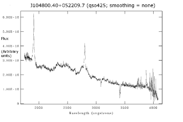
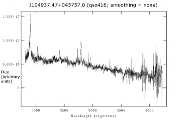
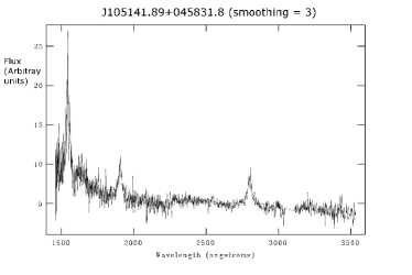
Figure 1: Example LQG spectra with a range of emission strengths from Hectopsec (J104947.34+041746.2 (qso412), J104800.40+052209.7 (qso425), and J104937.47+045757.0 (qso416) shown) and SDSS (J105141.89+045831.8 shown). All spectra can be found online.

2.2 LQG FIELD SAMPLE

Two LQGs and an additional quasar set have been found in the area studied in this paper. The overdensity was estimated using $(\rho-\langle\rho\rangle)/\langle\rho\rangle$ (CCGS12).

1. L1.28: The CCLQG lies at $z$ = [1.187,1.423], contains 34 members, and has an estimated overdensity of 0.83 and a statistical significance of 3.57$\sigma$ (CCGS12).

2. L1.11: There is another LQG at $z$ = [1.004,1.201], containing 38 members (CCGS12). This group has an estimated overdensity of 0.55 and a statistical significance of 2.95$\sigma$.

3. L1.54: There is an “enhanced set” of quasars with 21 members at $z$ = [1.477,1.614]. This group has an overdensity of 0.49, and a statistical significance of 1.75$\sigma$, which though suggestive, is not high enough to be statistically significant for a large structure (Newman 1999, CCGS12).

The original LQG members were selected from the SDSS DR7QSO catalogue (Schneider et al., 2010). A magnitude cut of $i$-mag = 19.1 (Schneider et al., 2010) was applied to create a uniform sample and quasars are within a 3D linking length of 100 Mpc. A convex hull is created around the members, giving the total volume covered by the LQG. See CCGS12 for more details on the method used to select LQG members.

The latest discussion of these LQGs can be found in CCGS12. Due to uncertainties over LQG membership caused by the member selection criteria and sample completeness, for the rest of the paper we will not be discussing the LQG or which quasars are classed as members. We will assume that quasars trace the mass distribution and therefore this area space and redshift range is therefore a candidate overdense region. Martini et al. (2013, and references therein) found for $1<z<1.5$ the fraction of AGN lying in clusters is increased compared to lower redshifts, making this a reasonable assumption.

There are 10 quasars at $1.1<z<1.7$ from the SDSS DR7 QSO catalogue (Schneider et al., 2010) which have SDSS spectra in the area of the LQGs we are studying. The spectra cover the wavelength range 3800–9200 Å and have a resolution of 2.5 Å (SDSS project book, 1999).

To improve statistics and better sample the overdensity, we increased the sample size. We start with a sample of quasars with photometric redshifts from the DR7 catalogue by Richards et al. (2009) which place them within the redshift range of the LQGs. We then randomly selected a subset of 32 for followup spectroscopy (observed as part of a larger observing project), dependent on available fiber positioning. We used the Hectospec instrument (Fabricant et al., 2005) a multi-object optical spectrograph, mounted at the 6.5-m MMT on Mount Hopkins, Arizona. The spectra were taken over nine nights and, due to inaccuracies in photometric redshifts, produced 18 quasar spectra within the required redshift range. The remaining objects were a mixture of quasars (generally at lower redshifts) and star forming galaxies.

The Hectospec data cover 3900 to 9100 Å and have a resolution of 1.2 Å. These spectra were reduced using the IDL based pipeline, HSRED. Table 1 shows the dates, fields, and exposures times for the Hectospec observations.

Table 1: Observing log for the Hectospec data.

Date	RA (J2000)	Dec (J2000)	Exposure (s)
17.02.2010	10:50:16.9	+04:37:12	5400
18.02.2010	10.50:16.9	+04:37:12	5400
19.02.2010	10:50:06.9	+04:29:16	5094
06.04.2010	10:50:06.9	+04:29:16	5400
07.04.2010	10:48:31.8	+05:23:29	7200
09.04.2010	10:48:31.8	+05:23:29	5400
10.04.2010	10:48:38.9	+05:25:57	5400
11.04.2010	10:48:38.9	+05:25:57	5400
11.04.2010	10:49:57.0	+04:30:01	5400
12.04.2010	10:49:57.0	+04:30:01	1800

The final catalogue of quasars (see Table 2) contains 18 quasars from Hectospec and 6 quasars from SDSS spectra within the redshift range $1.1<z<1.7$. Four of the SDSS quasars were removed due to low signal-to-noise spectra but are included in Table 2 for completeness. The area occupied by these quasars covers 1.6 deg² of the LQGs. An example of the spectra is shown in Fig. 1.

2.2.1 COMPLETENESS AND LQG MEMBERS

The Hectospec quasars, though not a complete sample, were randomly selected across area and redshift range, with no bias towards strong or weak Fe ii emission, magnitude, or location (beyond being within the field of the LQG overdensities). The quasars were observed as part a larger project which observed lower redshift luminous red galaxies. Therefore there was no biasing on the placement of the available fibers for observing these quasars.

Because of the data and the above described member selection method, we can say which quasars are part of the LQG as it is defined in CCGS12 but can not say whether these are the only members. If the sample used to determine members were complete down to the magnitude of $g$-mag = 21.1 (limit of the Hectospec data), additional members may be found and the shape of the convex hull would change.

For the purposes of this paper, we will assume that the LQGs indicate a general overdensity within this region. When mentioning the LQGs region, we refer to a region of space with a potential mass overdensity.

2.3 CONTROL SAMPLE

The control sample was taken from Stripe 82 from SDSS (York et al., 2000), which has a similar limiting magnitude (complete down to g-mag=21 to match the general completeness in the area of the LQGs) and taken from areas which do not contain any previously known LQGs. The samples were run through the program used to find the LQG and were determined not to be within a LQG within a 2$\sigma$ significance. We took multiple two deg² samples across the length of the stripe to reduce the impact of any marginal overdensities in a single area. The initial sample contains in total 394 field quasars within the redshift range $1.1<z<1.7$.

The errors were estimated across a range of objects and compared to the measured SNR. Spectra with SNR$<5$ per pixel rest EW had errors of $\pm$ 8.4 Å. This decreases to $\pm$ 4.8 Å for $5<$ SNR $<10$ per pixel and $\pm$ 2.85 Å for SNR $>10$ per pixel. Therefore, to reduce the effects of errors in measurements due to low SNR, spectra with an average SNR $<$ 5 per pixel were rejected. This removes four quasars from the LQGs field leaving 24, and reduces the control sample to 178 quasars, removing more control quasars due to generally lower SNR in SDSS spectra. The rejected quasars cover a range of W2400 EW values and do not favour any strength.

Fig. 2 shows the distribution of W2400 EW as a function of the $g$ band magnitude for both the control sample (circles, red) and the LQG field quasars (triangles, blue). Though some of the Hectospec quasars are fainter than the control sample quasars, there is no obvious relation between the magnitude and the W2400 EW emission. This is discussed further in section 4.

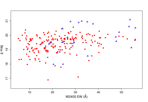
Figure 2: Comparison of the distribution of W2400 EW (Å) as a function of g magnitude for the quasars in the LQGs field (triangles, blue online) and control samples (circles, red online).

Table 2: Properties of the Hectospec quasars along with the properties for any other quasars within the 1.6 deg² field from the SDSS DR7QSO catalogue (Schneider et al., 2010). The columns show the Fe ii group, names, RA, DEC, redshift, LQG membership, Fe ii measurements using the method described in Weymann et al. (1991), and the $g$-magnitude, taken from SDSS. The asterisk on the quasar ID indicates previously known LQG members. L1.11 denotes the group with $\overline{z}=1.11$ (CCGS12), L1.28 for the group with $\overline{z}=1.28$ (CCGS12) and L1.54 indicates the additional quasar set at $\overline{z}=1.54$ (unpublished data).

Group	Quasar	Redshift	RA (J2000)	DEC (J2000)	membershipa	W2400b (Å)	g-mag
Ultra-strong	SDSS J104947.34+041746.2/qso412	1.159	10:49:47.35	+04:17:46.35	L1.11	56.08	20.51
	SDSS J104800.40+052209.7/qso425	1.230	10:48:00.41	+05:22:09.90	L1.28	56.01	19.70
	SDSS J104914.32+041428.6*	1.607	10:49:14.33	+04:14:28.65	L1.54	54.34	19.14
	SDSS J104930.44+054046.1/qso27	1.315	10:49:30.46	+05:40:46.20	L1.28	53.75	21.08
	SDSS J104815.93+055007.8/qso421	1.665	10:48:15.94	+05:50:07.80		53.32	20.60
	SDSS J104926.83+042334.6/qso417	1.653	10:49:26.83	+04:23:34.80		49.03	20.21
	SDSS J104921.05+050948.3/qso29	1.417	10:49:21.07	+05:09:48.30		47.78	19.58
	SDSS J105131.95+045124.7/qso41	1.434	10:51:31.94	+04:51:24.90		47.53	19.88
Strong	SDSS J104958.91+042723.3/qso217	1.622	10:49:58.92	+04:27:23.40	L1.54	37.64	20.79
	SDSS J105010.05+043249.1/qso48*	1.217	10:50:10.06	+04:32:49.20	L1.28	35.33	18.56
	SDSS J104933.41+054840.3/qso219	1.349	10:49:34.71	+05:48:36.00	L1.28	35.15	20.93
	SDSS J105255.65+055112.9c	1.678	10:52:55.65	+05:51:12.93		32.8	20.03
	SDSS J104937.47+045757.0/qso416	1.154	10:49:37.48	+04:57:57.10		32.72	20.98
Average	SDSS J105000.36+045157.8/qso410	1.418	10:50:00.36	+04:51:57.90		31.39	20.88
	SDSS J105154.14+041059.5c	1.552	10:51:54.14	+04:10:59.55	L1.54	29.94	21.29
	SDSS J105141.89+045831.8*	1.608	10:51:41.91	+04:58:27.90	L1.54	29.42	19.52
	SDSS J105007.90+043659.7/qso49	1.131	10:50:07.90	+04:36:59.70	L1.11	28.46	19.42
	SDSS J105036.09+045608.3/qso45	1.317	10:50:36.10	+04:56:11.40	L1.28	27.81	20.95
	SDSS J105352.75+043055.0/qso22	1.216	10:50:30.77	+04:30:55.05	L1.28	26.5	19.85
	SDSS J104656.71+054150.3*	1.228	10:46:56.71	+05:41:50.25	L1.28	24.57	17.99
	SDSS J104751.88+043709.9	1.696	10:47:51.89	+04:37:09.90		24.49	19.51
	SDSS J104840.85+040938.3/qso420	1.238	10:48:40.85	+04:09:38.55		24.42	20.46
	SDSS J105249.68+040046.3c	1.193	10:52:49.68	+04:00:46.50	L1.11	24.12	19.27
	SDSS J104932.22+050531.7/qso26*	1.111	10:49:32.23	+05:05:31.50	L1.11	23.16	18.84
	SDSS J104733.16+052454.9*	1.334	10:47:33.17	+05:24:55.05	L1.28	20.42	17.98
	SDSS J104943.28+044948.8/qso413	1.295	10:49:43.30	+04:49:48.75	L1.28	19.37	19.53
	SDSS J104938.35+052932.0*c	1.517	10:49:38.35	+05:29:31.95	L1.54	18.83	19.48
	SDSS J105018.10+052826.4*	1.307	10:50:18.12	+05:28:26.40	L1.28	18.46	19.39

$a.$ The membership is decided by quasar redshift and its inclusion within a convex hull created from the list of previously known members.
$b.$ Though the values can not be measured to this number of significant figures due to errors, the data has been left at two decimal places in order to remove the problems of ties in the data when running the Mann-Whitney test (described further in Section 3.2).
$c.$ These quasars are within the area of the LQGs and additional candidate overdensity. However, they will not be included in the statistics due to low signal-to-noise in the spectra.

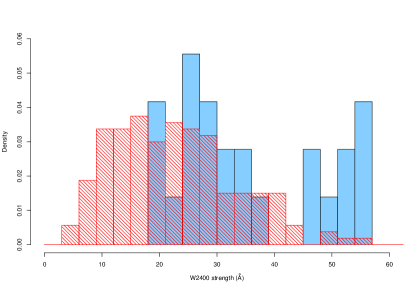
Figure 3: Normalised histogram (bin size= 3Å) showing the distribution of the measured W2400 EW density for the LQGs field (solid, blue online, 24 objects) and the control sample (hatched, red online, 178 objects).

3 RESULTS

Table 2 summarises the data for the sample. The quasars with an SDSS name as well as qsoXXX are those quasars selected from the photometric catalogue and re-observed using Hectospec. The spectra for these objects is available in the online material for this paper. The four quasars removed from the LQG sample due to low SNR have been included for completeness (denoted by “c”) but are not included in the analysis.

Table LABEL:tab:sample_props shows the median, mean and standard deviation of the control and LQGs samples. These data were used to define boundaries; the representative average range for the Fe ii equivalent width was taken as 10 - 32 Å, anything between 32 and 43 Å EW was classed as strong and greater than 43 Å EW was classed as ultra-strong Fe ii.

Using this system, eight quasars were classed as ultra-strong and four were classed as strong Fe ii emitters from a sample size of 24 quasars within 1.6 deg², in the redshift interval of $1.1<z<1.7$.

3.1 A SIGNIFICANT DIFFERENCE IN THE DISTRIBUTION OF ULTRA-STRONG EMITTERS

Table LABEL:tab:cont_samples shows the number of quasars (and percentage) with different UV Fe ii strengths in the LQGs field and the control fields. We show both the complete sample and a magnitude limited sample where all the quasars are within the same magnitude range ($17.98<g<20.56$). The LQGs field has a large percentage of quasars with strong and ultra-strong Fe ii emission. 33.3 $\pm~{}11.8$ per cent of the LQG field sample show ultra-strong Fe ii emission and 16.7 $\pm~{}8.3$ per cent show strong emission. This compares to the control sample which has 3.4 $\pm~{}1.4$ per cent of quasars showing ultra-strong emission and 15.7 $\pm~{}3.1$ per cent showing strong emission. Thus there is a statistical difference for the ultra-strong emitting quasars, which is also seen to the magnitude limited samples. For the magnitude limited samples, the percentage of strong quasars in the LQG field drops to 5.9 $\pm~{}5.9$ per cent, compared to the control sample value of 16.0 $\pm~{}3.0$ per cent, which are no longer within the errors.

However as the definitions of strong and ultra-strong are arbitrary and dependent on the control sample, for the rest of the paper, we will concentrate on the differences in the full distribution from the data and control samples.

Table 3: Median, mean and standard deviation of W2400 EW (Å) for the LQG sample and SDSS control sample.

Sample	median	mean	standard
			deviation
control sample	21.20	22.59	10.86
LQG field	32.05	35.71	12.71

Table 4: The number of quasars per deg² for the different Fe ii strengths for quasars in the control fields (covering a total area of 26 deg²) compared to the LQGs field (which cover 1.6 deg²). The percentages are those of the total in the field. The magnitude limited sample has the magnitude range $17.98<g<20.56$.

	Complete		Mag. Limited
Strength	LQGs field	control field	LQGs field	control field
Ultra-strong	5.0 (33.3%)	0.23 (3.37%)	3.75 (35.3%)	0.23 (3.45%)
Strong	2.5 (16.7%)	1.08 (15.7%)	0.63 (5.9%)	1.08 (16.2%)
Average	7.5 (50.0%)	4.78 (69.7%)	6.25 (58.8%)	4.62 (69.4%)
Weak	0.0 (0.0%)	0.77 (11.2%)	0.0 (0.0%)	0.73 (11.0%)

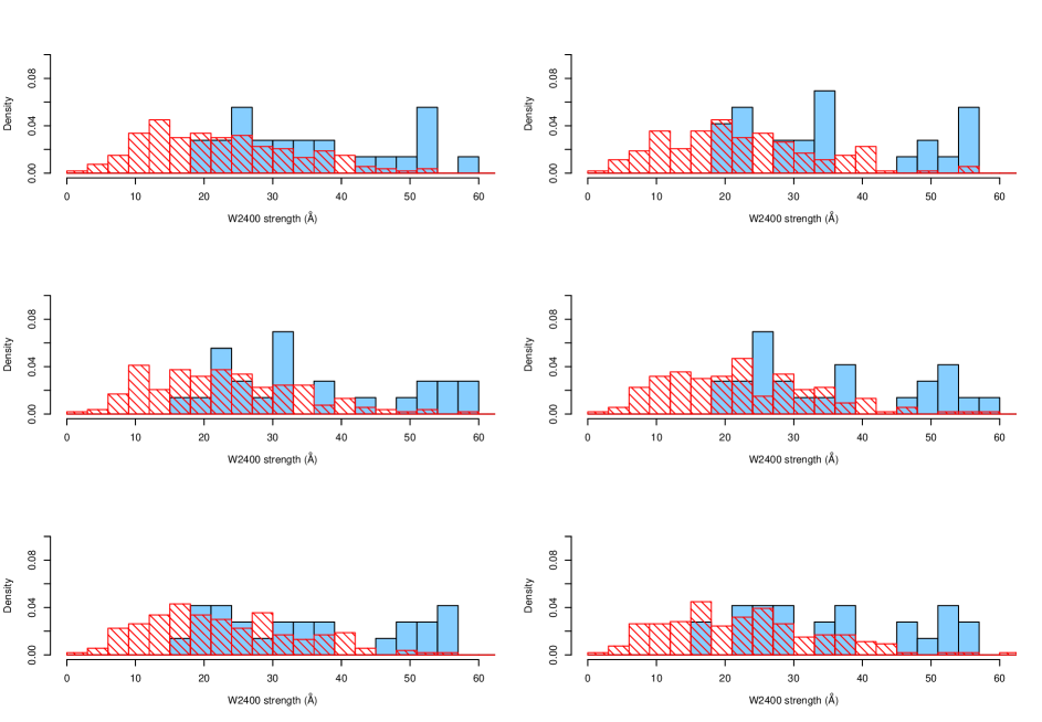
Figure 4: Example histograms (bin size = 3Å) showing six possible distributions within the errors of the measurements taken from the Monte-Carlo re-sampling. The histograms shows the distribution of the measured W2400 EW for the LQGs field (solid, blue online, 24 objects) and the control sample (hatched, red online, 178 objects).

3.2 W2400 distribution

Fig.  3 (bin size= 3 Å) shows the distribution of the W2400 EW for the LQGs field (solid, blue online) and the control sample (hatched, red online). The relative excess of UV Fe ii emission in the LQGs field can be clearly seen for W2400 EW $>45$ Å. For W2400 EW $<20$ Å, the histogram shows the lack of low emission quasars within the LQGs field compared to the control sample. Fig. 4 shows a selection of histograms from a Monte-Carlo method. For each histogram, a point is randomly selected for each object across the whole distribution with appropriate weighting. This figure shows at the upper end of the emission, there is again an excess of quasars with W2400 $>$ 45, indicating this result is not affected by the errors. There is also a lack at W2400 $<$ 20 Å.

To quantify the difference in distributions, we employ the Mann-Whitney test, a powerful non-parametric test for comparing two populations. The Mann-Whitney test does not require any assumptions about the forms of the distributions, and is less likely to apply significance to outliers due to the ranking method used. This test is however sensitive to rounding, which can create ties in ranks in the data, therefore we have measured to two decimal places, though the data is not accurate to this level, and do not rounded our data at any point (DeGroot, 1986). Median latencies in the LQG field and control sample are 32.05 and 21.20 respectively. Using a one-tailed Mann-Whitney test, with 24 LQG quasars and 178 control sample quasars, the distributions in the two groups differ significantly with a p-value of 99.996%.

To estimate the effects of the errors on the W2400 measurements, a Monte-Carlo method was used to resample points from within the error limits for each measurement across the whole distribution with appropriate weighting and Mann-Whitney test repeated, using the same parameters as above. In each case, P $<$ 0.05. Therefore taking into account errors, the two distributions are still differ significantly.

To investigate the lack of weak Fe ii emitting (W2400 $<$ 20 Å) which could be due to the limit sample size, the Mann-Whitney statistical test was repeated using the samples with only W2400 $>$ 20 Å. This test gives P = $0.013\pm~{}0.05$, indicating that removing the weak emitters does have a significant effect on the result. However, this artificially truncates the values, creating an artificial distribution. To properly test this lack of weak emitters, a larger sample of quasars within overdense regions would be needed.

4 DISCUSSION

We have shown there is an increase in the Fe ii emission within quasars within the LQGs compared to our control sample. There are various possible explanations:

1. a selection effect - created by the selection of LQG quasars and magnitude limits,

2. dust - different amounts of dust within the LQG sample and the control sample causing the difference in the observed EW distributions,

3. Ly$\alpha$ fluorescence - Ly$\alpha$ pumping can cause an increase the Fe ii,

4. microturbulence - motions within the cloud line emitting region,

5. iron abundance - an enhanced Milky Way-like star formation creating an increased iron abundance.

We do not believe the observed distribution differences are due to selection effects. The quasars observed with Hectospec were randomly selected from the photometric catalogues. The control sample was selected to match the redshift and magnitude distributions of LQG quasars. However, there is a slight difference in the magnitude ranges, due to the magnitude limit of SDSS, shown in Fig. 2. Seven quasars within the LQG are fainter than the control sample by $<$ 0.5 magnitudes. However, the correlation between UV Fe ii and the quasar luminosity is still debated. Some studies have found an inverse Baldwin effect in the optical Fe ii emission, with the EW Fe ii emission increasing with the continuum emission (Kovačević et al., 2010; Dong et al., 2011; Han et al., 2011). For the UV Fe ii, no significant correlation has been observed between the UV Fe ii and the quasar luminosity or $L/L_{Edd}$ (Dong et al., 2011; Sameshima et al., 2009).

To investigate any effect of the magnitude on our data, a magnitude limit of $17.98<g<20.56$ was applied to both samples. The Mann-Whitney test gives a P = 0.0007 showing that even with a magnitude-limited sample which further limits the sample size, the distributions of the LQGs field and control samples are still different.

The second possible explanation is an difference in dust properties between the LQG and the control sample causes the differences observed. As an excess of dust in the LQG region would reduce the UV emission, we do not believe this difference is due to dust emission. For dust emission to have an effect on our results, the control sample would have to see evidence of an steeper extinction law. However as the control sample consists of quasars from 13 different areas, it would require large scale special dust properties with the LQG field, which is unlikely. Since there is now a consensus that higher rates of star formation are seen in overdense environments at z $>$ 1 (e.g. Farrah et al., 2006; Amblard et al., 2011), we think it very unlikely that ISM dust is the cause of this difference, since if dust were causing the effect we’d expect the very high EW systems to be found in the field.

The third and fourth options are Ly$\alpha$ fluorescence and microturbulence, which are additional mechanisms within the BLR believed to increase the Fe ii emission. Again we do not believe this is the case as the control sample was selected to have similar quasar properties. As mentioned above, the small differences in magnitude are unlikely to be the cause of the distribution differences.

An increase in Ly$\alpha$ emission can cause an increase in the UV Fe ii emission (Sigut & Pradhan, 2003; Sigut et al., 2004; Verner et al., 2004). As the width of the Ly$\alpha$ increases, it overlaps with numerous Fe ii lines within the wavelength range 1212-1218 Å. These lines are excited, and when they decay produce emission in the UV Fe ii region, 2200-2700 Å. Increasing the Ly$\alpha$ emission will therefore increase the UV Fe ii emission. In fact, Sigut & Pradhan (1998) found that Ly$\alpha$ fluorescent excitation can more than double the UV Fe ii flux.

Low resolution $R\sim 90$ GALEX UV spectra which cover the Ly$\alpha$ emission exist for six of the quasars (program GI5-059, Williger et al.). Fig. 5 shows the correlation between the Fe ii EW measurements and the equivalent widths of the Ly$\alpha$ emission line. The line drawn is the weighted (using both sets of errors) least squares best-fit. The Pearson correlation coefficient between the Ly$\alpha$ and the Fe ii is 0.830 $\pm~{}0.14$. There is a suggestive trend for quasars with higher Ly$\alpha$ emission to have stronger Fe ii emission, as predicted (e.g Sigut & Pradhan, 2003; Sigut et al., 2004; Verner et al., 2004). However, there are only six spectra here with GALEX Ly$\alpha$ emission. This fit is highly dependent on the presence of qso425 (which has the largest W2400 EW) and not robust.

Though the Ly$\alpha$ emission may influence the observed Fe ii emission, there is no reason to believe the quasars within the LQG field have increased Ly$\alpha$ emission compared to randomly selected quasars. However, more data of quasar Ly$\alpha$ emission in various environments would be needed to fully investigate this. Equally with an overdense environments, the effect of other quasars and nearby galaxies is negligible compared to the emission from the accretion disc of the quasar.

The Fe ii flux strength can also be increased by microturbulence around the AGN (Vestergaard & Wilkes, 2001; Sigut & Pradhan, 2003; Sigut et al., 2004; Verner et al., 2003, 2004; Bruhweiler & Verner, 2008). Microturbulence (non-thermal random motions within a cloud’s line emitting region; Bottorff & Ferland 2000; Bottorff et al. 2000) spreads the line absorption coefficient over a larger wavelength range (Bruhweiler & Verner, 2008), broadens the Ly$\alpha$ emission lines, and therefore increases the UV Fe ii emission observed. Microturbulence is occurs within the BLR. Large scale dynamic effects due to the large scale environment are unlikely to have an affect on the BLR without causing observable differences in the host galaxy, such star formation rates and luminosity, which is not seen here as our control was designed to match the field sample.

Although these factors have been shown to influence the UV Fe ii emission, modelling needs to be completed for quasars in environment over a range of densities to study how Ly$\alpha$ fluorescence and microturbulence can change with environment.

The final option is that the observed difference is due to the host galaxy and the quasars simply illuminate this difference. As previously noted, the dependence of metallicity with environment is still highly debated, with some studies showing a weak but significant trend for galaxies in higher density regions (such as groups or clusters) to have higher metallicities. Therefore if, as we assume the quasars in LQGs trace the overdense regions, we would expect the host galaxies to have greater metallicities.

Galaxies with old stellar populations have been found to favour higher density environments at z $\sim$ 0 (e.g. Balogh et al., 2004; Blanton et al., 2005) and z $\sim$ 1 (e.g. Cooper et al., 2006). Martini et al. (2013) found AGN have evolved more rapidly in higher density environments than the field population. This suggests, at high redshifts, star formation may occur in high density environments (e.g. Cooper et al., 2008). If so, this will increase the metals available in the vicinity of these quasars. To produce the observed Fe ii (assuming abundance is the main factor), the hosts would have gone through a period of enhanced star formation between $2<z<3$, assuming it takes between 0.3 Gyr and 1 Gyr (Hamann & Ferland, 1993) for the required number of SNeIa to occur to create significant amounts of iron. This is during the peak epoch of star formation (e.g Lilly et al., 1996; Madau et al., 1996; Sobral et al., 2013).

There is no significant enhancement in Mg ii in the LQG quasars compared to the control sample. This is consistant with a Milky Way-like star formation as opposed to a starburst. A increase in quiescent star formation in some of the galaxies within the LQGs would produce an increase in the iron abundance with respect to the Mg ii.

Within an overdense region, there could also be additional metal enrichment of the quasars from supernovae occurring the inter-cluster medium and within nearby galaxies. Supernovae have been shown to efficiently enrich the IGM over Mpc scales (e.g. Domainko et al., 2004; Adelberger et al., 2005). These metals may then accrete the quasar, further enriching the quasar host.

5 SUMMARY

There is a increase in Fe ii emission in a candidate overdense region, indicating there may be a build up of iron. It is consistant with an increase in star formation in overdense region at high redshift. This star formation must have occurred at 2 $<$ z $<$ 3 for iron to be observed in these quasars. Additionally surrounding galaxies in this dense region will release metals into the IGM, which can fall onto the quasar, producing an observed metal increase.

This will make published LQGs interesting regions in which to study the evolution of metals in high density regions and at high redshifts.

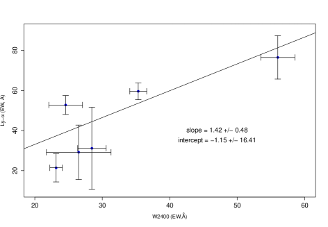
Figure 5: Comparing the equivalent widths for the Fe ii emission from the optical spectra and the Ly$\alpha$ emission from GALEX UV spectra. The line fitted shows Ly$\alpha$_EW = W2400_EW, fit using least squares weighted regression.

6 Acknowledgments

KAH would like to acknowledge and thank the STFC, the University of Central Lancashire and the Obs. de la Côte d’Azur for their funding, and hospitality. Also KAH would like thank Roger Clowes and Luis Campusano for their communications

This research uses data from the Hectospec instrument on the MMT.

The authors acknowledge support from the NASA GALEX program GI5-059, grant NNX09AQ13G.

This research has used the SDSS DR7QSO catalogue (Schneider et al., 2010). Funding for the SDSS and SDSS-II has been provided by the Alfred P. Sloan Foundation, the Participating Institutions, the National Science Foundation, the U.S. Department of Energy, the National Aeronautics and Space Administration, the Japanese Monbukagakusho, the Max Planck Society, and the Higher Education Funding Council for England. The SDSS Web Site is http://www.sdss.org/.

The SDSS is managed by the Astrophysical Research Consortium for the Participating Institutions. The Participating Institutions are the American Museum of Natural History, Astrophysical Institute Potsdam, University of Basel, University of Cambridge, Case Western Reserve University, University of Chicago, Drexel University, Fermilab, the Institute for Advanced Study, the Japan Participation Group, Johns Hopkins University, the Joint Institute for Nuclear Astrophysics, the Kavli Institute for Particle Astrophysics and Cosmology, the Korean Scientist Group, the Chinese Academy of Sciences (LAMOST), Los Alamos National Laboratory, the Max-Planck-Institute for Astronomy (MPIA), the Max-Planck-Institute for Astrophysics (MPA), New Mexico State University, Ohio State University, University of Pittsburgh, University of Portsmouth, Princeton University, the United States Naval Observatory, and the University of Washington.

References

- Adelberger et al. (2005) Adelberger K.L., Shapley A.E., Steidel C.C., Pettini M., Erb D.K., Reddy N.A., 2005, ApJ, 629, 636
- Amblard et al. (2011) Amblard, A. et al., 2011 Nature, 470, 510A
- Baldwin et al. (2004) Baldwin J.A., Ferland G.J., Korista K.T., Hamann F., LaCluyzé A., 2004, ApJ, 615, 610
- Balogh et al. (2004) Balogh M.L., Baldry I.K., Nichol R., Miller C., Bower R., Glazebrook K., 2004, ApJ, 615, 101
- Blain et al. (2004) Blain A.W., Chapman S.C., Smail I., Ivison R., 2004, ApJ, 611, 725
- Blanton et al. (2005) Blanton M.R., Eisenstein D., Hogg D.W., Schlegel D.J., Brinkmann J., 2005, ApJ, 629, 143
- Bottorff & Ferland (2000) Bottorff M.C., Ferland G.J., 2000a, MNRAS, 316, 103
- Bottorff et al. (2000) Bottorff M., Ferland G., Baldwin J., Korista K., 2000b, ApJ, 542, 644
- Bruhweiler & Verner (2008) Bruhweiler F., Verner E., 2008, ApJ, 675, 82
- Clowes & Campusano (1991) Clowes R.G., Campusano L.E., 1991, MNRAS, 249, 218
- Clowes & Campusano (1994) Clowes R.G., Campusano L.E., 1994, MNRAS, 266, 317
- Clowes et al. (2012) Clowes R.G., Campusano L.E., Graham M.J., Söchting I.K., 2012, MNRAS, 419, 556
- Cooper et al. (2006) Cooper M.C. et al. 2006, MNRAS, 370, 198
- Cooper et al. (2008) Cooper M.C., Tremonti C.A., Newman J.A., Zabludoff A.I., 2008, MNRAS, 390, 245
- Cooper et al. (2013) Cooper H.D.B. et al. 2013, MNRAS, 430, 1125
- DeGroot (1986) DeGroot M.H., 1986, Probability and Statistics (2nd ed.; Addison-Wesley Publishing company Inc.)
- Domainko et al. (2004) Domainko W., Gitti M., Schindler S., Kapferer W., 2004, A&A, 425, 21
- Dong et al. (2011) Dong X.-B., Wang J.-G., Ho L. C., Wang T.-G., Fan X., Wang H., Zhou H., Yuan W., 2011, ApJ, 736, 86
- Elitzur & Netzer (1985) Elitzur M., Netzer H., 1985, ApJ, 291, 464
- Fabricant et al. (2005) Fabricant D. et al. 2005, PASP, 117, 1411
- Farrah et al. (2006) Farrah D. et al., 2006, ApJ, 641, 17
- Gómez et al. (2003) Gómez P.L. et al., 2003, ApJ, 584, 210
- Graham et al. (1996) Graham M., Clowes R.G., Campusano L.E., 1996, MNRAS, 279, 1349
- Johansson & Jordan (1984) Johansson S., Jorda C., 1984, MNRAS, 210, 239
- Hamann & Ferland (1993) Hamann F., Ferland G., 1993, ApJ, 418, 11
- Han et al. (2011) Han X., Wang J., Wei J., Yang D., Hou J., 2011, ScChG, 54, 346
- Hartig & Baldwin (1986) Hartig G.F., Baldwin J.A., 1986, ApJ, 302, 64
- Hartman & Johansson (2000) Hartman H., Johansson S., 2000, A&A, 359, 627
- Hughes et al. (2013) Hughes T.M., Cortese L., Boselli A., Gavazzi G., Davies J.I., 2013, A&A, 550, 115
- Komberg et al. (1996) Komberg B.V, Kravtsov A.V., Lukash V.N., 1996, MNRAS, 282, 713
- Kovačević et al. (2010) Kovačević J, Popović L.Č., Dimitrijević M.S., 2010, ApJS, 189, 15
- Lilly et al. (1996) Lilly S. J., Le Fevre O., Hammer F., Crampton D., 1996, ApJ, 460, 1
- Madau et al. (1996) Madau P., Ferguson H.C., Dickinson M.E., Giavalisco M., Steidel C.C., Fruchter A., 1996, MNRAS, 283, 1388
- Martini et al. (2013) Martini P. et al., 2013, ApJ, 768, 1
- Matsuoka et al. (2007) Matsuoka Y., Oyabu S., Tsuzuki Y., Kawara K., 2007, ApJ, 663, 781
- Netzer & Wills (1983) Netzer H., Will B.J., 1983, ApJ, 275, 445
- Newman (1999) Newman P.R., 1999, PhD Thesis, University of Central Lancashire
- Osterbrock (1976) Osterbrock D.E., 1976, ApJ, 203, 329
- Osterbrock & Ferland (2006) Osterbrock D.E., Ferland G.J., 2006, Astrophysics of Gaseous Nebulae and Active Galactic Nuclei (2nd ed.; University Science books)
- Richards et al. (2009) Richards G.T. et al., 2009, ApJS, 180, 67
- Sameshima et al. (2009) Sameshima H. et al., 2009, MNRAS, 395, 1087
- Sameshima et al. (2011) Sameshima H., Kawara K., Matsuoka Y., Oyabu S., Asami N., Ienaka N., 2011, MNRAS, 410, 1018
- Schneider et al. (2010) Schneider D.P., et al., 2010, AJ, 139, 2360
-
SDSS project book (1999)
The
Astrophysical Research Consortium, Princeton,
http://www.astro.princeton.edu/PBOOK/welcome.htm - Sigut & Pradhan (1998) Sigut T.A.A., Pradhan A.K., 1998, ApJ, 499, 139
- Sigut & Pradhan (2003) Sigut T.A.A., Pradhan A.K., 2003, ApJS, 145, 15
- Sigut et al. (2004) Sigut T.A.A, Pradhan A.K, Nahar S.N., 2004, ApJ, 611, 81
- Skillman et al. (1996) Skillman E.D., Kennicutt Jr. R.C., Shields G.A., Zaritsky D., 1996, ApJ, 462, 147
- Sobral et al. (2013) Sobral D., Smail I., Best P.N., Geach J.E., Matsuda Y., Stott J.P., Cirasuolo M., Kurk J., 2013, MNRAS, 428, 1128
- Verner et al. (2003) Verner E., Bruhweiler F., Verner D., Johansson S., Gull T., 2003,ApJ, 592, 59
- Verner et al. (2004) Verner E., Bruhweiler F., Verner D., Johansson S., Kallman T., Gull, T., 2004, ApJ, 611, 780
- Vestergaard & Wilkes (2001) Vestergaard M., Wilkes B.J., 2001, ApJS, 134, 1
- Weymann et al. (1991) Weymann R.J., Morris S.L., Foltz C.B., Hewett P.C., 1991, ApJ, 373, 23
- Wray et al. (2006) Wray J.J., Bahcall N.A., Bode P., Boettiger C., Hopkins P.F., 2006, ApJ, 652, 907
- York et al. (2000) York D.G. et al., 2000, AJ, 120, 1579