Complex rotation numbers

Abstract.

We investigate the notion of complex rotation number which was introduced by V. I. Arnold in 1978. Let $f\colon{\mathbb{R}/\mathbb{Z}}\to{\mathbb{R}/\mathbb{Z}}$ be an orientation preserving circle diffeomorphism and let $\omega\in{\mathbb{C}/\mathbb{Z}}$ be a parameter with positive imaginary part. Construct a complex torus by glueing the two boundary components of the annulus $\Set{z\in{\mathbb{C}/\mathbb{Z}}}{0<\mathop{\mathrm{Im}}(z)<\mathop{\mathrm{Im}}(\omega)}$ via the map $f+\omega$. This complex torus is isomorphic to $\mathbb{C}/(\mathbb{Z}+\tau\mathbb{Z})$ for some appropriate $\tau\in{\mathbb{C}/\mathbb{Z}}$.

According to Moldavskis [6], if the ordinary rotation number $\operatorname{rot}(f+\omega_{0})$ is Diophantine and if $\omega$ tends to $\omega_{0}$ non tangentially to the real axis, then $\tau$ tends to $\operatorname{rot}(f+\omega_{0})$. We show that the Diophantine and non tangential assumptions are unnecessary: if $\operatorname{rot}(f+\omega_{0})$ is irrational then $\tau$ tends to $\operatorname{rot}(f+\omega_{0})$ as $\omega$ tends to $\omega_{0}$.

This, together with results of N.Goncharuk [4], motivates us to introduce a new fractal set (“bubbles”), given by the limit values of $\tau$ as $\omega$ tends to the real axis. For the rational values of $\operatorname{rot}(f+\omega_{0})$, these limits do not necessarily coincide with $\operatorname{rot}(f+\omega_{0})$ and form a countable number of analytic loops in the upper half-plane.

Notation:

• $\mathbb{H}=\mathbb{H}^{+}$ is the set of complex numbers with positive imaginary part.

• $\mathbb{H}^{-}$ is the set of complex numbers with negative imaginary part.

• If $p/q$ is a rational number, then $p$ and $q$ are assumed to be coprime.

• If $x$ and $y$ are distinct points in ${\mathbb{R}/\mathbb{Z}}$, then $(x,y)$ denotes the set of points $z\in{\mathbb{R}/\mathbb{Z}}-\set{x,y}$ such that the three points $x,z,y$ are in increasing order and $[x,y]{:=}(x,y)\cup\set{x,y}$.

• $\operatorname{rot}(f)\in{\mathbb{R}/\mathbb{Z}}$ is a rotation number of an orientation-preserving circle diffeomorphism $f$.

• If $f\colon{\mathbb{R}/\mathbb{Z}}\to{\mathbb{R}/\mathbb{Z}}$ is a circle diffeomorphism, $\displaystyle D_{f}{:=}\int_{{\mathbb{R}/\mathbb{Z}}}\left|\frac{f^{\prime\prime}(x)}{f^{\prime}(x)}\right|{\ {\rm d}}x.$

Introduction

Given an orientation preserving analytic circle diffeomorphism $f\colon{\mathbb{R}/\mathbb{Z}}\to{\mathbb{R}/\mathbb{Z}}$ and a parameter $\omega\in{\mathbb{H}/\mathbb{Z}}$, set

$$f_{\omega}{:=}f+\omega\colon{\mathbb{R}/\mathbb{Z}}\to{\mathbb{R}/\mathbb{Z}}+\omega.$$

The circles ${\mathbb{R}/\mathbb{Z}}$ and ${\mathbb{R}/\mathbb{Z}}+\omega$ bound an annulus $A_{\omega}\subset{\mathbb{C}/\mathbb{Z}}$. Glueing the two sides of $A_{\omega}$ via $f_{\omega}$, we obtain a complex torus $E(f_{\omega})$, which may be uniformized as $\cal{E}_{\tau}{:=}\mathbb{C}/(\mathbb{Z}+\tau\mathbb{Z})$ for some appropriate $\tau\in{\mathbb{H}/\mathbb{Z}}$, the homotopy class of ${\mathbb{R}/\mathbb{Z}}$ in $E(f_{\omega})$ corresponding to the homotopy class of ${\mathbb{R}/\mathbb{Z}}$ in $\cal{E}_{\tau}$. The complex rotation number of $f_{\omega}$ is $\tau_{f}(\omega){:=}\tau$. It is the complex analogue of the ordinary rotation number of $f+t$ for $t\in{\mathbb{R}/\mathbb{Z}}$.

V. I. Arnold’s problem [1], generalized by R. Fedorov and E. Risler independently, is to study the relation of the ordinary rotation number of the circle diffeomorphism $f\colon{\mathbb{R}/\mathbb{Z}}\to{\mathbb{R}/\mathbb{Z}}$ and the limit behaviour of the complex rotation number $\tau_{f}(\omega)$ as $\omega$ tends to $0$.

According to work of Risler [7, Chapter 2, Proposition 2], the function

$$\tau_{f}\colon{\mathbb{H}/\mathbb{Z}}\to{\mathbb{H}/\mathbb{Z}}$$

is holomorphic. We shall show that there is a continuous extension of $\tau_{f}$ to

$$\overline{{\mathbb{H}/\mathbb{Z}}}{:=}{\mathbb{H}/\mathbb{Z}}\cup{\mathbb{R}/\mathbb{Z}}.$$

The ordinary rotation number of a circle homeomorphism $f\colon{\mathbb{R}/\mathbb{Z}}\to{\mathbb{R}/\mathbb{Z}}$ is defined as follows. Let $F\colon\mathbb{R}\to\mathbb{R}$ be a lift of $f\colon{\mathbb{R}/\mathbb{Z}}\to{\mathbb{R}/\mathbb{Z}}$. Such a lift is unique up to addition of an integer. The sequence of functions $\frac{1}{n}\bigl{(}F^{\circ n}-{\rm id}\bigr{)}$ converges uniformly to a constant function $\Theta$. If we replace $F$ by $F+k$ with $k\in\mathbb{Z}$, the limit $\Theta$ is replaced by $\Theta+k$, so that the value $\operatorname{rot}(f)\in{\mathbb{R}/\mathbb{Z}}$ of $\Theta$ modulo $1$ only depends on $f$. This is the rotation number of $f$. Note that the rotation number is rational if and only if the circle homeomorphism has a periodic orbit.

Our main result, proved in Section 9, concerns the behavior of $\tau_{f}(\omega)$ as $\omega$ tends to ${\mathbb{R}/\mathbb{Z}}$. Recall that a periodic orbit of a circle diffeomorphism is called parabolic if its multiplier is 1, and it is called hyperbolic otherwise. A circle diffeomorphism with periodic orbits is called hyperbolic if it has only hyperbolic periodic orbits.

Main Theorem.

Let $f\colon{\mathbb{R}/\mathbb{Z}}\to{\mathbb{R}/\mathbb{Z}}$ be an orientation preserving analytic circle diffeomorphism. Then, the function $\tau_{f}\colon{\mathbb{H}/\mathbb{Z}}\to{\mathbb{H}/\mathbb{Z}}$ has a continuous extension $\bar{\tau}_{f}\colon\overline{{\mathbb{H}/\mathbb{Z}}}\to\overline{{\mathbb{H}/\mathbb{Z}}}$. Assume $\omega\in{\mathbb{R}/\mathbb{Z}}$.

• If $\operatorname{rot}(f_{\omega})$ is irrational, then $\bar{\tau}_{f}(\omega)=\operatorname{rot}(f_{\omega})$.

• If $\operatorname{rot}(f_{\omega})=p/q$ is rational, then $\bar{\tau}_{f}(\omega)$ belongs to the closed disk of radius $D_{f}/(4\pi q^{2})$ tangent to ${\mathbb{R}/\mathbb{Z}}$ at $p/q$; moreover

  • if $f_{\omega}$ has a parabolic cycle, then $\bar{\tau}_{f}(\omega)=\operatorname{rot}(f_{\omega})$.

  • if $f_{\omega}$ is hyperbolic, then $\bar{\tau}_{f}(\omega)\in{\mathbb{H}/\mathbb{Z}}$, in particular $\bar{\tau}_{f}(\omega)\neq\operatorname{rot}(f_{\omega})$.

Our main contribution to this result is the case of irrational (yet not Diophantine) rotation number, and the continuous extension of $\tau_{f}$ to the whole boundary ${\mathbb{R}/\mathbb{Z}}$. The particular case of this theorem:

Corollary 1.

If $\operatorname{rot}(f)$ is irrational, then $\tau_{f}(\omega)$ converges to $\operatorname{rot}(f)$ when $\omega$ goes to zero.

solves the problem posed by Étienne Ghys (however he refers to V.Arnold) [2, p. 25].

The case of Diophantine rotation numbers was investigated earlier by E.Risler [7, Chapter 2] and V.Moldavskis [6] independently. Risler constructed the map $\tau_{f}$ in a some subset $\Omega_{s}$ of ${\mathbb{H}/\mathbb{Z}}$; $\Omega_{s}$ is detached from points $\omega\in{\mathbb{R}/\mathbb{Z}}$ with $\operatorname{rot}(f_{\omega})\in\mathbb{Q}/\mathbb{Z}$. He also studied the behavior of $\tau_{f}$ and obtained some formulas and estimates on its derivatives; in particular, he proved that $\tau_{f}$ is injective on $\Omega_{s}$ provided that $f$ is close to rotation.

The case of parabolic cycles was studied by J.Lacroix (unpublished) and N.Goncharuk [4] independently. The case of hyperbolic diffeomorphisms was dealt first by Yu. Ilyashenko and V. Moldavskis [5], then this result was improved by N.Goncharuk [4]. For exact statements of these results, see Section 2.

In Appendix A, we shall also study the behavior of $\tau_{f}(\omega)$ as the imaginary part of $\omega$ tends to $+\infty$.

1. Bubbles: a new fractal set

The Main Theorem enables us to define a new interesting fractal set, related to the circle diffeomorphism, namely the set $\bar{\tau}_{f}({\mathbb{R}/\mathbb{Z}})$. Due to the Main Theorem, this set contains ${\mathbb{R}/\mathbb{Z}}$ and a countable number of loops — “bubbles”, the endpoints of bubbles are rational points of ${\mathbb{R}/\mathbb{Z}}$ (see the sketch in Fig. 1). Due to Theorem 8, these loops are analytic curves.

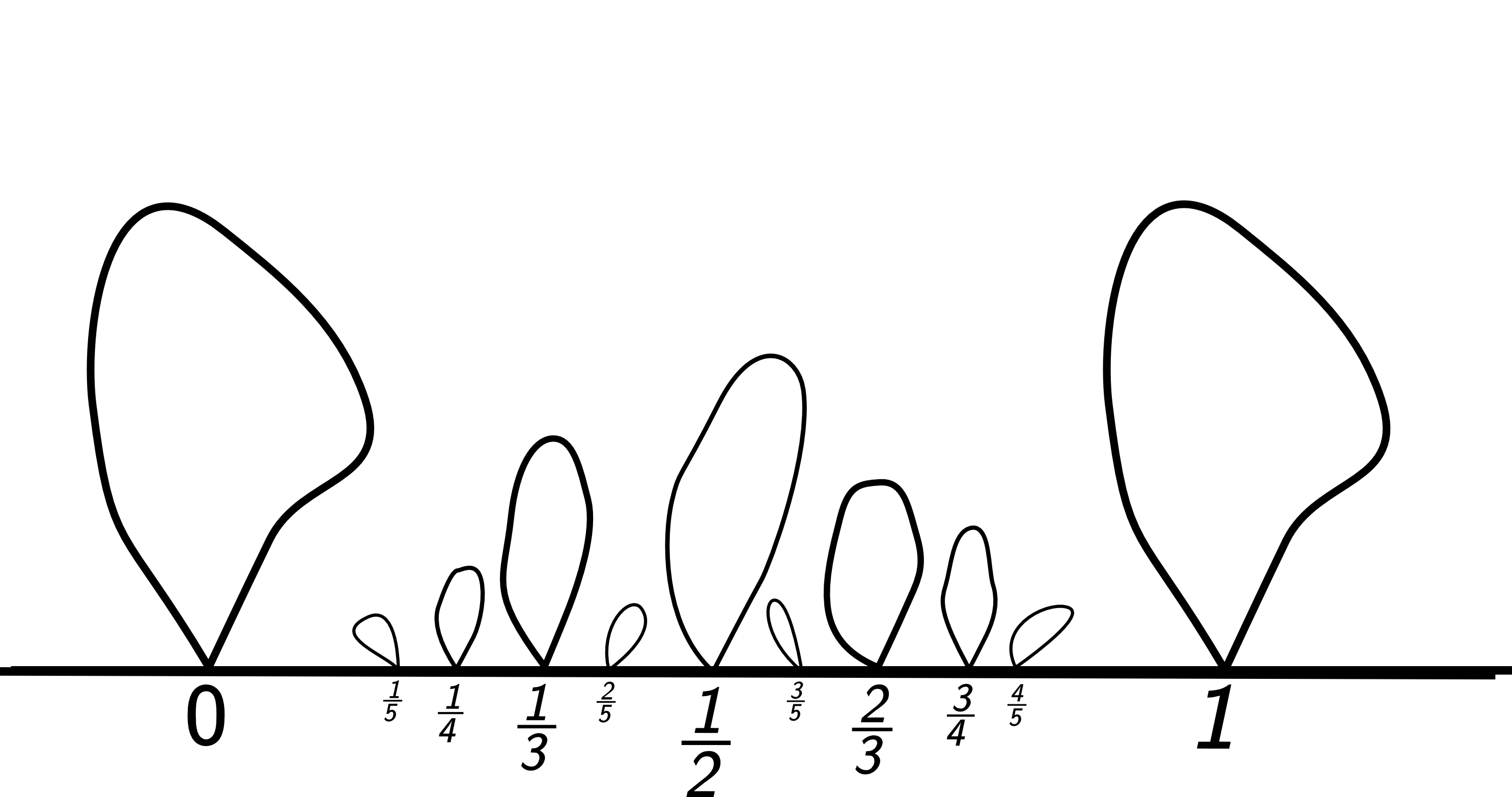
Figure 1. Bubbles. The sketch of the set $\bar{\tau}_{f}({\mathbb{R}/\mathbb{Z}})$.

There are many natural questions about the geometrical structure of the set $\bar{\tau}_{f}({\mathbb{R}/\mathbb{Z}})$:

1. Is it true that $\bar{\tau}_{f}({\mathbb{R}/\mathbb{Z}})$ is the boundary of $\tau_{f}({\mathbb{H}/\mathbb{Z}})$, and $\tau_{f}$ is univalent?

2. How large are bubbles?

3. Do different bubbles intersect each other?

4. What is the shape of a bubble? In particular, could a bubble be self-intersecting?

5. What can be said about the shape of a “bubble bundle”, when several bubbles grow from the same point of the real axis (see Fig. 5)?

We disprove the conjecture of item (1), see Corollary 6 at the end of this Section.

As for item (2), the following lemma is a part of Main Theorem:

Lemma 2.

(Size of bubbles) The bubble corresponding to $\operatorname{rot}(f_{\omega})=p/q$ belongs to the disk tangent to ${\mathbb{R}/\mathbb{Z}}$ at $p/q$ with radius $C/q^{2}$, where $C=D_{f}/(4\pi)$. If $f$ is $C^{1}-$close to a rotation, then $C$ is close to $0$.

This implies that when $f$ is close to a rotation, different bubbles do not intersect (item (3)).

The question on the shape of bubbles (item (4)) is still open, however our results clarify the shape of bubbles near their endpoints. Let us introduce the following classification:

Definition.

If all maps $f_{\omega},\omega\in(\omega_{0},\omega_{0}+\varepsilon]$ are hyperbolic, and $f_{\omega_{0}}$ is not, then $\omega_{0}$ is called a (left) endpoint of a bubble. In this case, $\bar{\tau}_{f}(\omega)\to\operatorname{rot}(f_{\omega_{0}})$ as $\omega\to\omega_{0},\omega>\omega_{0}$, due to the continuity of $\bar{\tau}_{f}(\omega)$.

If the multiplier of some fixed point of $f_{\omega}$ tends to one as $\omega\to\omega_{0},\omega>\omega_{0}$, then $\omega_{0}$ is called a real (left) endpoint of a bubble. For example, this happens if some parabolic cycle of $f_{\omega_{0}}$ bifurcates into real hyperbolic cycles as $\omega$ increases.

If the multipliers of fixed points of $f_{\omega}$ do not tend to one as $\omega\to\omega_{0},\omega>\omega_{0}$, then $\omega_{0}$ is called a complex (left) endpoint of a bubble. This means that all parabolic cycles of $f_{\omega_{0}}$ bifurcate into complex conjugate cycles as $\omega$ increases. Note that in this case, $f_{\omega_{0}}$ must have other hyperbolic cycles, otherwise $f_{\omega},\omega\in(\omega_{0},\omega_{0}+\varepsilon]$ cannot be hyperbolic.

In an analogous way, we introduce the notion of right endpoints of bubbles.

Lemma 3.

(Real endpoints) If $\omega_{0}$ is a real endpoint of the bubble, $\operatorname{rot}(f_{\omega_{0}})=p/q$, then the curve $\bar{\tau}_{f}(\omega),\,\omega\to\omega_{0},\omega>\omega_{0}$, tends to $p/q\in{\mathbb{R}/\mathbb{Z}}$ from above: enters any horocycle at the point $p/q$, see Fig. 2 (a).

Lemma 4.

(Complex endpoints) If $\omega_{0}$ is a complex endpoint of the bubble, $\operatorname{rot}(f_{\omega_{0}})=p/q$, then the curve $\bar{\tau}_{f}(\omega),\,\omega\to\omega_{0},\omega>\omega_{0}$, is located between two horocycles at $p/q$.

For the left endpoint, this curve is tangent to the segment $[p/q,p/q+\varepsilon)$, see Fig. 2 (b). For the right endpoint, it will be tangent to the segment $(p/q-\varepsilon,p/q]$.

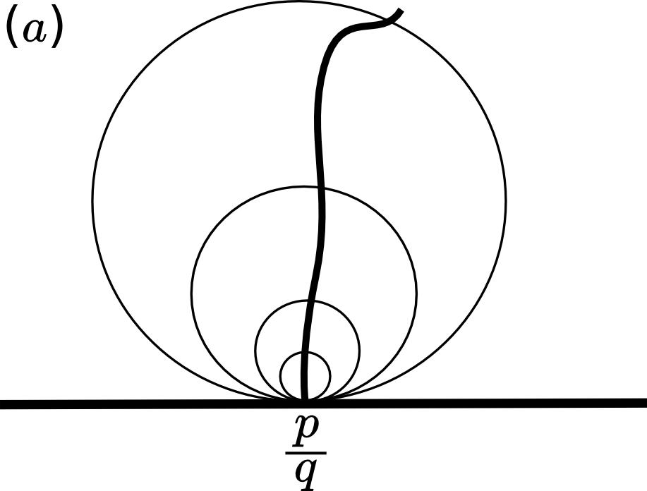
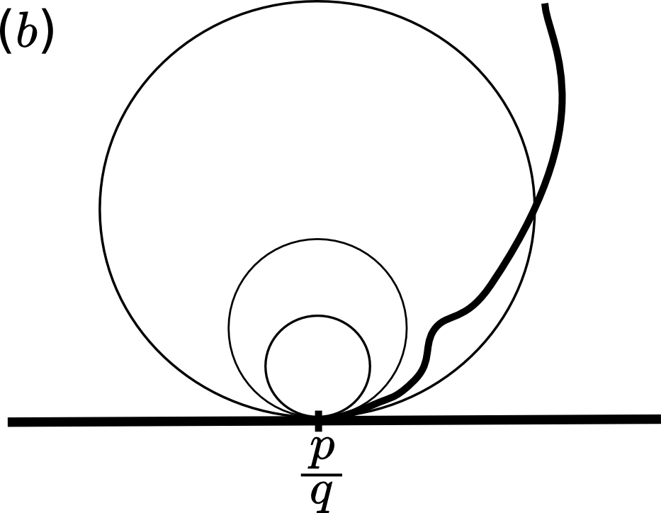
Figure 2. The sketch of the curve $\bar{\tau}_{f}(\omega)$, $\omega\in[\omega_{0},\omega_{0}+\varepsilon]$, in the case when $\omega_{0}$ is (a) real and (b) complex left endpoint of the bubble; $\operatorname{rot}(f_{\omega_{0}})=\frac{p}{q}$.

Remark 5.

When we pass to the diffeomorphism $x\mapsto-f(-x)$, the map $\bar{\tau}_{f}$ is conjugated by $z\mapsto-\bar{z}$. Thus it is sufficient to prove Lemmas 3 and 4 only for left endpoints.

We finish this section by Corollary 6 which disproves the conjecture of item (1).

Corollary 6.

Assume that $x-f(x)$ has two local maxima at points $x_{1}$ and $x_{2}$ with $x_{1}-f(x_{1})\neq x_{2}-f(x_{2})$ (see Fig. 3). Then, $\tau_{f}$ is not injective.

Proof.

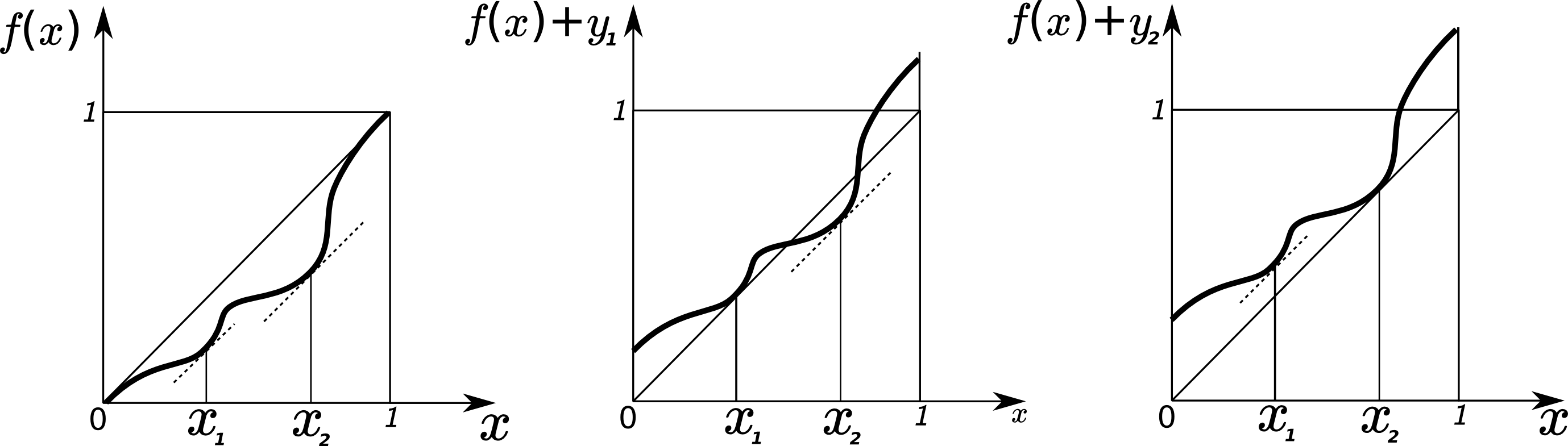
Figure 3. Graphs of the functions $f,f+y_{1},f+y_{2}$.

Let $y_{1}$ and $y_{2}$ be the respective values of $x-f(x)$ at $x_{1}$ and $x_{2}$. Suppose that $y_{1}<y_{2}$. Then the map $f_{\omega}$ for $y_{1}<\omega<y_{2}$ has zero rotation number, and it has parabolic fixed points for $\omega=y_{1}$ and $\omega=y_{2}$. Note that when $\omega$ increases from $y_{1}$ to $y_{1}+\varepsilon$, the parabolic fixed point disappears ($y_{1}$ is a complex left endpoint of a bubble), thus due to Lemma 4, the curve $\omega\mapsto\bar{\tau}_{f}(\omega)$ is tangent to $[0,0+\varepsilon)$. When $\omega<y_{2}$ tends to $y_{2}$, the two hyperbolic fixed points merge into a parabolic fixed point ($y_{2}$ is a real endpoint of a bubble). Thus, according to Lemma 3, the curve $\omega\mapsto\bar{\tau}_{f}(\omega)$ enters any horocycle at $0$ as $\omega<y_{2}$ tends to $y_{2}$. Fig. 4 shows the sketch of this bubble. But if $\tau_{f}$ were injective, the pair of germs of the curve $\bar{\tau}_{f}|_{{\mathbb{R}/\mathbb{Z}}}$ at $y_{1}$ and $y_{2}$ (both passing through $0$) would be oriented clockwise. The contradiction shows that $\tau_{f}$ is not injective in the upper half-plane. ∎

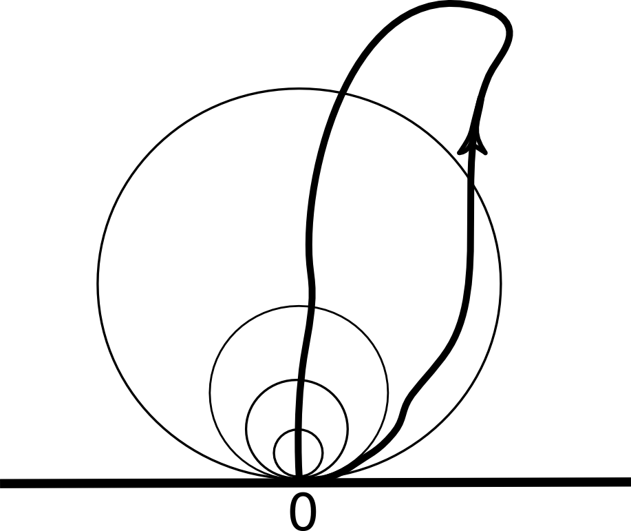
Figure 4. The sketch of the curve $\bar{\tau}_{f}((y_{1},y_{2}))$.

For the map $f$ whose graph is shown in Fig. 3, the same arguments give some information about the curve $\bar{\tau}_{f}((0,y_{2}))$ — the bubble bundle (see item (5)). However we cannot choose between numerous possible pictures, see Fig. 5 for two of them. The question on the exact shape of a bubble bundle stays open.

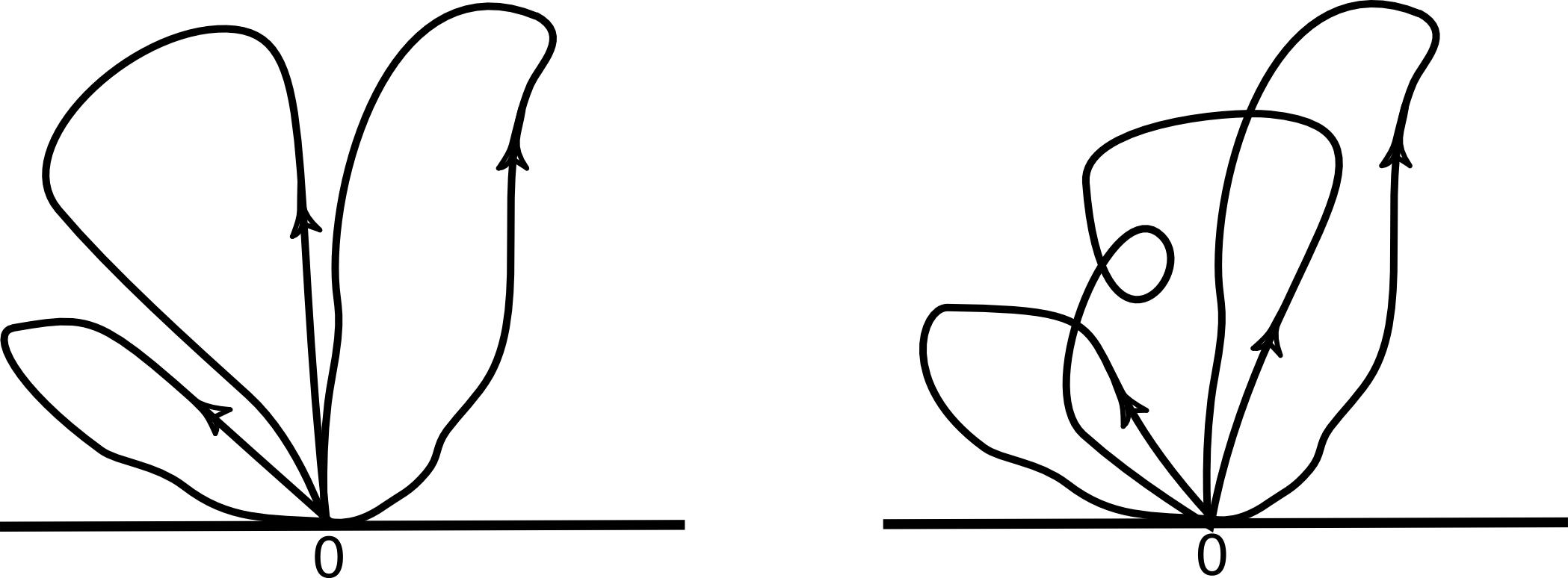
Figure 5. The “bubble bundle”: the possible sketches of the curve $\bar{\tau}_{f}((0,y_{2}))$.

2. Strategy of the proof

The proof of the Main Theorem goes as follows.

Step 1. Recall that a number $\theta\in{\mathbb{R}/\mathbb{Z}}$ is Diophantine if there are constants $c>0$ and $\beta>0$ such that for all rational numbers $p/q\in\mathbb{Q}/\mathbb{Z}$, we have

$$\left|x-\frac{p}{q}\right|>\frac{c}{q^{2+\beta}}.$$

Theorem 7 (V. Moldavskis [6]).

If $\omega\in{\mathbb{R}/\mathbb{Z}}$ and if $\operatorname{rot}(f_{\omega})$ is Diophantine, then

$$\lim_{\begin{subarray}{c}y\to 0\\ y>0\end{subarray}}\tau_{f}(\omega+{\rm i}y)=\operatorname{rot}(f_{\omega}).$$

Theorem 7 was proved by Risler [7] as a corollary of a very delicate analog of the Arnold–Hermann theorem. A very short direct proof was obtained by Moldavskis [6].

Step 2.  If $\omega\in{\mathbb{R}/\mathbb{Z}}$ and $\operatorname{rot}(f_{\omega})$ is rational, then the conclusion of Theorem 7 is not true. This fact was first proved by Yu. Ilyashenko and V. Moldavkis [5]. We do not formulate their result since we will use its later generalized version.

Theorem 8 (N. Goncharuk [4]).

If $\omega\in{\mathbb{R}/\mathbb{Z}}$, if $\operatorname{rot}(f_{\omega})$ is rational and if $f_{\omega}$ is hyperbolic, then $\tau_{f}$ extends analytically to a neighborhood of $\omega$.

In the following, we shall denote by $\bar{\tau}_{f}(\omega)$ this extension of $\tau_{f}$ at $\omega$. At this stage, $\bar{\tau}_{f}(\omega)$ is defined on a countable number of real segments. However, in what follows we will define $\bar{\tau}_{f}$ on the whole ${\mathbb{R}/\mathbb{Z}}$.

Step 3. Recall that $\theta\in{\mathbb{R}/\mathbb{Z}}$ is Liouville if it is irrational but not Diophantine. We use the following result of Tsujii.

Theorem 9 (M. Tsujii [8]).

The set of $\omega\in{\mathbb{R}/\mathbb{Z}}$ such that $\operatorname{rot}(f_{\omega})$ is Liouville has zero Lebesgue measure.

It implies that almost every $\omega\in\mathbb{R}/\mathbb{Z}$ satisfies assumptions of either Theorem 7, or Theorem 8 (note that the set of $\omega$ such that $f_{\omega}$ has a parabolic cycle is countable, because our family is analytic).

Step 4. If $f_{\omega}$ has rational rotation number, we usually denote it by $p/q$. We denote by $\operatorname{Per}(f_{\omega})$ the set of periodic points of $f_{\omega}\colon{\mathbb{R}/\mathbb{Z}}\to{\mathbb{R}/\mathbb{Z}}$. For $x\in\operatorname{Per}(f_{\omega})$, we denote by $\rho_{x}$ the multiplier of $x$ as a fixed point of $f^{\circ q}$. Our contribution starts with the following result. It is an analog of the Yoccoz Inequality which bounds the multiplier of a fixed point of a polynomial in terms of its combinatorial rotation number [3].

Lemma 10.

Assume that $f_{\omega}$ is a hyperbolic map with rational rotation number $p/q$. Then, $\bar{\tau}_{f}(\omega)$ belongs to the disk tangent to ${\mathbb{R}/\mathbb{Z}}$ at $p/q$ with radius

(1) $$R_{\omega}{:=}\frac{1}{2\displaystyle\pi q\cdot\sum_{x\in\operatorname{Per}(f_{\omega})}\frac{1}{|\log\rho_{x}|}}.$$

In addition,

(2) $$R_{\omega}\leq D_{f}/(4\pi q^{2}).$$

The cardinal of $\operatorname{Per}(f_{\omega})$ for a hyperbolic map is at least $2q$, and according to Lemma 13, for each $x\in\operatorname{Per}(f_{\omega})$ we have $|\log\rho_{x}|\leq D_{f}$. Thus the estimate (1) yields (2).

Estimate (2) immediately implies Lemma 2.

Note that Lemma 10 implies Lemma 3. Indeed, for real endpoints of bubbles, one of the multipliers $\rho_{x}$ tends to 1, and (1) yields that $R_{\omega}$ tends to $0$ as $\omega\to 0$. Thus $\bar{\tau}_{f}(\omega)$ enters any horocycle at $p/q$.

Step 5. Let $\bar{\tau}_{f}\colon{\mathbb{R}/\mathbb{Z}}\to{\mathbb{C}/\mathbb{Z}}$ be defined by

• $\bar{\tau}_{f}(\omega){:=}\operatorname{rot}(f_{\omega})$ if the rotation number of $f_{\omega}$ is irrational or if $f_{\omega}$ has a parabolic cycle and

• $\displaystyle\bar{\tau}_{f}(\omega){:=}\lim_{\begin{subarray}{c}y\to 0\\ y>0\end{subarray}}\tau_{f}(\omega+{\rm i}y)$ if $f_{\omega}$ is hyperbolic.

This definition agrees with the definition of $\bar{\tau}_{f}(\omega)$ for hyperbolic $f_{\omega}$ (see section 2). We are going to prove that $\bar{\tau}_{f}$ is the continuous extension of $\tau_{f}$ to the real axis; so the coincidence of the notation with that of Main Theorem is not accidental and will not lead to confusion.

Lemma 11.

(Continuity of the boundary function) The function $\bar{\tau}_{f}$ is continuous on ${\mathbb{R}/\mathbb{Z}}$.

It is particularly difficult to prove the continuity of $\bar{\tau}_{f}$ at complex endpoints of bubbles. For the points $\omega$ where $f_{\omega}$ is hyperbolic (points of bubbles), it follows from Theorem 8; for real endpoints of bubbles, we use Lemma 3; for the points with irrational $\operatorname{rot}(f_{\omega})$, we need Lemma 2.

Step 6. The holomorphic map $\tau_{f}\colon{\mathbb{H}/\mathbb{Z}}\to{\mathbb{H}/\mathbb{Z}}$ has radial limits on ${\mathbb{R}/\mathbb{Z}}$ almost everywhere, and those limits coincide with the continuous map $\bar{\tau}_{f}$. It follows easily that $\tau_{f}$ extends continuously by $\bar{\tau}_{f}$ to ${\mathbb{R}/\mathbb{Z}}$.

3. Multipliers of periodic orbits and distortion

Before embarking into the proof of our results, we shall obtain the useful estimate on multipliers of periodic orbits of a circle diffeomorphism (Lemma 13).

The distortion of a diffeomorphism $f\colon I\to J$ is

$$\operatorname{dis}_{I}(f)=\max_{x,y\in I}\log\frac{f^{\prime}(x)}{f^{\prime}(y)}.$$

If $f\colon I\to J$ and $g\colon J\to K$ are diffeomorphisms, then

$$\operatorname{dis}_{J}(f^{-1})=\operatorname{dis}_{I}(f)\quad\text{and}\quad\operatorname{dis}_{I}(g\circ f)\leq\operatorname{dis}_{I}(f)+\operatorname{dis}_{J}(g).$$

Lemma 12 (Denjoy).

Let $f\colon{\mathbb{R}/\mathbb{Z}}\to{\mathbb{R}/\mathbb{Z}}$ be an orientation preserving diffeomorphism and $I\subset{\mathbb{R}/\mathbb{Z}}$ be an interval such that $I$, $f(I)$, $f^{\circ 2}(I)$, …, $f^{\circ n}(I)$ are disjoint. Then,

$$\operatorname{dis}_{I}(f^{\circ n})\leq D_{f}.$$

Proof.

Let $x$ and $y$ be points in $I$. Set $x_{k}{:=}f^{\circ k}(x)$ and $y_{k}{:=}f^{\circ k}(y)$. Then,

$$\bigl{|}\log(f^{\circ n})^{\prime}(x)-\log(f^{\circ n})^{\prime}(y)\bigr{|} =\left|\sum_{k=0}^{n-1}\log f^{\prime}(x_{k})-\log f^{\prime}(y_{k})\right|$$

$$\leq\sum_{k=0}^{n-1}\left|\int_{x_{k}}^{y_{k}}\frac{f^{\prime\prime}(x)}{f^{\prime}(x)}{\ {\rm d}}x\right|\leq\int_{\mathbb{R}/\mathbb{Z}}\left|\frac{f^{\prime\prime}(x)}{f^{\prime}(x)}\right|{\ {\rm d}}x=D_{f}.\qed$$

As a corollary, we have the following control on the multipliers of the periodic orbits of $f$. This result is surely known by specialists, but we include its proof due to the lack of a suitable reference.

Lemma 13.

(Estimate on multipliers) Let $f\colon{\mathbb{R}/\mathbb{Z}}\to{\mathbb{R}/\mathbb{Z}}$ be an orientation preserving diffeomorphism and $\rho$ be the multiplier of a cycle of $f$. Then, $|\log\rho|\leq D_{f}$.

Proof.

The average of the derivative $(f^{\circ q})^{\prime}$ along the circle ${\mathbb{R}/\mathbb{Z}}$ is equal to $1$. As a consequence, there exists a point $x_{0}\in{\mathbb{R}/\mathbb{Z}}$ such that $(f^{\circ q})^{\prime}(x_{0})=1$. Any periodic orbit $\set{x,f(x),\dots,f^{\circ q}(x)=x}$ divides the circle into disjoint intervals $I_{1},\dots,I_{q}$ which are permuted by $f$. Without loss of generality, we may assume that $I_{1}$ contains $x$ and $x_{0}$. Then, according to the previous Lemma,

$$|\log\rho|=\bigl{|}\log(f^{\circ q})^{\prime}(x)\bigr{|}=\left|\log\frac{(f^{\circ q})^{\prime}(x)}{(f^{\circ q})^{\prime}(x_{0})}\right|\leq\operatorname{dis}_{I_{1}}(f^{\circ q})\leq D_{f}.\qed$$

4. The Diophantine case

We include a proof of Theorem 7. It is a simplified version of original proof of Moldavskis [6].

The proof relies on the following lemma on quasiconformal maps which is classical.

Lemma 14.

Suppose that there exists a $K$-quasiconformal map between two complex tori $E_{1}$ and $E_{2}$. Then

$$\operatorname{dist}_{\mathbb{H}}(\tau(E_{1}),\tau(E_{2}))\leq\log K$$

where $\operatorname{dist}_{\mathbb{H}}$ is the hyperbolic distance in $\mathbb{H}$, and where $\tau(E_{1})\in\mathbb{H}$ and $\tau(E_{2})\in\mathbb{H}$ are moduli with respect to corresponding generators in $H_{1}(E_{1})$ and $H_{1}(E_{2})$.

Without loss of generality, we may assume that $\omega=0$, so $f\colon{\mathbb{R}/\mathbb{Z}}\to{\mathbb{R}/\mathbb{Z}}$ has Diophantine rotation number $\theta\in{\mathbb{R}/\mathbb{Z}}$. A theorem of Yoccoz (see [9]) asserts that there is an analytic circle diffeomorphism $\phi\colon{\mathbb{R}/\mathbb{Z}}\to{\mathbb{R}/\mathbb{Z}}$ conjugating the rotation of angle $\theta$ to $f$: for all $x\in{\mathbb{R}/\mathbb{Z}}$, we have

$$\phi(x+\theta)=f\circ\phi(x).$$

Let $\hat{\phi}\colon{\mathbb{C}/\mathbb{Z}}\to{\mathbb{C}/\mathbb{Z}}$ be the homeomorphism defined by

$$\hat{\phi}(z)=\phi\bigl{(}\mathop{\mathrm{Re}}(z)\bigr{)}+{\rm i}\mathop{\mathrm{Im}}(z).$$

Then, $\hat{\phi}\colon{\mathbb{C}/\mathbb{Z}}\to{\mathbb{C}/\mathbb{Z}}$ is a $K$-quasiconformal homeomorphism with

$$K{:=}\max\bigl{(}\|\phi^{\prime}\|_{\infty},\|1/\phi^{\prime}\|_{\infty}\bigr{)}.$$

Now, for any $y>0$,

$$\hat{\phi}(x+\theta+{\rm i}y)=f\bigl{(}\hat{\phi}(x)\bigr{)}+iy,$$

and so, $\hat{\phi}$ induces a $K$-quasiconformal homeomorphism between the complex tori $\mathbb{C}/\bigl{(}\mathbb{Z}+(\theta+{\rm i}y)\mathbb{Z}\bigr{)}$ and $E(f_{{\rm i}y})$. It follows that for $y>0$, the hyperbolic distance in ${\mathbb{H}/\mathbb{Z}}$ between $\theta+{\rm i}y$ and $\tau_{f}({\rm i}y)$ is uniformly bounded and thus,

$$\lim_{\begin{subarray}{c}y\to 0\\ y>0\end{subarray}}\tau_{f}({\rm i}y)=\theta.$$

5. The hyperbolic case: formation of bubbles

We recall the arguments of the proof of Theorem 8 given in [4]. It is based on an auxiliary construction of a complex torus $\mathfrak{E}(f)$ when $f\colon{\mathbb{R}/\mathbb{Z}}\to{\mathbb{R}/\mathbb{Z}}$ has rational rotation number and is hyperbolic. This construction will be used again in the proofs of Lemmas 2, 3, 4, and 10 for $f_{\omega}$ playing the role of $f$.

Let us assume $f\colon{\mathbb{R}/\mathbb{Z}}\to{\mathbb{R}/\mathbb{Z}}$ has rational rotation number $p/q$ and has only hyperbolic periodic orbits. The number $m\geq 1$ of attracting cycles is equal to the number of repelling cycles. Denote by $\alpha_{j}$, $j\in\mathbb{Z}/(2mq)\mathbb{Z}$, the periodic points of $f$, ordered cyclically; even indices correspond to attracting periodic points and odd indices to repelling periodic points. Note that $f(\alpha_{j})=\alpha_{j+2mp}$.

Let $\rho_{j}$ be the multiplier of $\alpha_{j}$ as a fixed point of $f^{\circ q}$ and $\phi_{j}\colon(\mathbb{C},0)\to({\mathbb{C}/\mathbb{Z}},\alpha_{j})$ be the linearizing map which conjugates multiplication by $\rho_{j}$ to $f^{\circ q}$:

$$f^{\circ q}\circ\phi_{j}(z)=\phi_{j}(\rho_{j}z)$$

and is normalized by $\phi_{j}^{\prime}(0)=1$. Then,

$$f\circ\phi_{j}(z)=\phi_{j+2mp}(\lambda_{j}\cdot z)\quad\text{with}\quad\lambda_{j}{:=}f^{\prime}(\alpha_{j}).$$

In addition, if $\varepsilon>0$ is small enough, the linearizing map $\phi_{j}$ extends univalently to the strip $\Set{z\in\mathbb{C}}{{|\mathop{\mathrm{Im}}(z)|<\varepsilon}}$ and

$$\phi_{j}(\mathbb{R})=(\alpha_{j-1},\alpha_{j+1}).$$

For each $j\in\mathbb{Z}/(2mq)\mathbb{Z}$, let $x_{j}$ be a point in $(\alpha_{j},\alpha_{j+1})$, so that

• $f(x_{j})\in(\alpha_{j+2pm},x_{j+2pm})$ if the orbit of $\alpha_{j}$ attracts (i.e. $j$ is even) and

• $f(x_{j})\in(x_{j+2pm},\alpha_{j+2pm+1})$ if the orbit of $\alpha_{j}$ repels (i.e. $j$ is odd).

This is possible since $f^{\circ q}(x_{j})\in(\alpha_{j},x_{j})$ when $j$ is even and $f^{\circ q}(x_{j})\in(x_{j},a_{j+1})$ when $j$ is odd. Similarly, let $\varepsilon_{j}$ be a point on the negative imaginary axis if $j$ is even and on the positive imaginary axis if $j$ is odd, so that for all $j\in\mathbb{Z}/(2mq\mathbb{Z})$,

• $|\varepsilon_{j}|<\varepsilon$, $|\lambda_{j}\varepsilon_{j}|<\varepsilon$ and

• $\lambda_{j}\varepsilon_{j}$ is above $\varepsilon_{j+2mp}$.

Let $C_{j}$ be the arc of circle with endpoints $\phi_{j}^{-1}(x_{j-1})$ and $\phi_{j}^{-1}(x_{j})$ passing through $\varepsilon_{j}$ and set

$$\gamma{:=}\bigcup_{j\in\mathbb{Z}/(2mq\mathbb{Z})}\phi_{j}(C_{j}).$$

Then, $\gamma$ is a simple closed curve in ${\mathbb{C}/\mathbb{Z}}$ and $f$ is univalent in a neighborhood of $\gamma$.

Figure 6. A possible choice of curve $\gamma$ for the map $f\colon{\mathbb{C}/\mathbb{Z}}\ni z\mapsto z+\frac{1}{4\pi}\sin(2\pi x)\in{\mathbb{C}/\mathbb{Z}}$ which restricts as a hyperbolic circle diffeomorphism $f\colon{\mathbb{R}/\mathbb{Z}}\to{\mathbb{R}/\mathbb{Z}}$. The curve $f(\gamma)$ lies above $\gamma$ in ${\mathbb{C}/\mathbb{Z}}$. The essential annulus between $\gamma$ and $f(\gamma)$ is colored (light grey in the upper half-plane and dark grey in the lower half-plane). The map $f$ has an attracting fixed point at $\alpha_{0}{:=}0\in{\mathbb{R}/\mathbb{Z}}$ and a repelling fixed point at $\alpha_{1}{:=}1/2\in{\mathbb{R}/\mathbb{Z}}$.

The attracting cycles of $f$ are above $\gamma$ in ${\mathbb{C}/\mathbb{Z}}$ and the repelling cycles are below $\gamma$ in ${\mathbb{C}/\mathbb{Z}}$. In addition,

$$f(\gamma)=\bigcup_{j\in\mathbb{Z}/(2mq\mathbb{Z})}\phi_{j+2mp}(\lambda_{j}C_{j})$$

and so, $f(\gamma)$ lies above $\gamma$ in ${\mathbb{C}/\mathbb{Z}}$.

For $\omega$ sufficiently close to $0$, the curve $f_{\omega}(\gamma)=f(\gamma)+\omega$ remains above $\gamma$ in ${\mathbb{C}/\mathbb{Z}}$. The curves $\gamma$ and $f_{\omega}(\gamma)$ bound an essential annulus in ${\mathbb{C}/\mathbb{Z}}$. Glueing the two sides via $f_{\omega}$, we obtain a complex torus $\mathfrak{E}(f_{\omega})$, which may be uniformized as $\cal{E}_{\tau}{:=}\mathbb{C}/(\mathbb{Z}+\tau\mathbb{Z})$ for some appropriate $\tau\in{\mathbb{H}/\mathbb{Z}}$, the homotopy class of $\gamma$ in $\mathfrak{E}(f_{\omega})$ corresponding to the homotopy class of ${\mathbb{R}/\mathbb{Z}}$ in $\cal{E}_{\tau}$. Clearly, $\mathfrak{E}(f_{\omega})$ does not depend on the choice of $\varepsilon_{j}$. We set $\bar{\tau}_{f}(\omega){:=}\tau\in{\mathbb{H}/\mathbb{Z}}$.

According to Risler [7, Chapter 2, Proposition 2], the map $\omega\mapsto\bar{\tau}_{f}(\omega)$ is holomorphic. When $\omega\in{\mathbb{H}/\mathbb{Z}}$, the complex torus $\mathfrak{E}(f_{\omega})$ is isomorphic to $E(f_{\omega})$ and the homotopy class of $\gamma$ in $\mathfrak{E}(f_{\omega})$ corresponds to the homotopy class of ${\mathbb{R}/\mathbb{Z}}$ in $E(f_{\omega})$ (see [4] for details; in some sense, $E(f_{iy})$ is a limit case of $\mathfrak{E}(f_{iy})$ as $\varepsilon_{j}$ tend to zero and $\gamma$ tends to the real axis). As a consequence, $\bar{\tau}_{f}(\omega)=\tau_{f}(\omega)$ when $\omega\in{\mathbb{H}/\mathbb{Z}}$ is sufficiently close to $0$. This completes the proof of Theorem 8 for $\omega=0$: the map $\bar{\tau}_{f}$ extends $\tau_{f}$ analytically to a neighborhood of zero, as required.

Remark 15.

Note that the curve $\mathfrak{E}(f)$ does not depend on the choice of an analytic chart on a circle: $\bar{\tau}_{f}(0)=\bar{\tau}_{gfg^{-1}}(0)$ for any orientation-preserving analytic circle diffeomorphism $g$. So we can give the description of $\mathfrak{E}(f)$ in terms of moduli of analytic conjugation, that is, in terms of the multipliers of the fixed points and the transition maps between the linearizing charts $\phi_{j}$. This description is given at the beginning of Section 7.

We will also need a following observsation:

Lemma 16.

The modulus of $\mathfrak{E}(f^{\circ q})$ is $q$ times bigger then the modulus of $\mathfrak{E}(f)$: $\bar{\tau}_{f^{\circ q}}(0)=q\bar{\tau}_{f}(0)$.

Proof.

The diffeomorphism $f$ induces an automorphism of $\mathfrak{E}(f^{\circ q})$ of order $q$. The quotient of $\mathfrak{E}(f^{\circ q})$ by this automorphism is isomorphic to $\mathfrak{E}(f)$. The class of $\gamma$ in $\mathfrak{E}(f)$ has $q$ disjoint preimages in $\mathfrak{E}(f^{\circ q})$ which map with degree $1$ to $\gamma$. It follows that $\mathfrak{E}(f^{\circ q})$ is isomorphic to ${\cal E}_{q\bar{\tau}_{f}(0)}{:=}\mathbb{C}/(\mathbb{Z}+q\bar{\tau}_{f}(0)\mathbb{Z})$, the class of $\gamma$ in $\mathfrak{E}(f^{\circ q})$ corresponding to the class of ${\mathbb{R}/\mathbb{Z}}$ in ${\cal E}_{q\bar{\tau}_{f}(0)}$. ∎

6. Lemma 2 (size of bubbles) and Lemma 3 (continuity at the real endpoints)

We now come to our main contribution, starting with the proof of Lemma 10. Assume $f_{\omega}\colon{\mathbb{R}/\mathbb{Z}}\to{\mathbb{R}/\mathbb{Z}}$ has rational rotation number $p/q$ and has only hyperbolic periodic orbits. For simplicity of notation, we put $\omega=0$ and write $f=f_{0}$ instead of $f_{\omega}$. As in Section 5, consider a simple closed curve $\gamma$ oscillating between the attracting cycles of $f$ (which are above $\gamma$ in ${\mathbb{C}/\mathbb{Z}}$) and the repelling cycles of $f$ (which are below $\gamma$ in ${\mathbb{C}/\mathbb{Z}}$), so that $f(\gamma)$ lies above $\gamma$ in ${\mathbb{C}/\mathbb{Z}}$.

The curves $\gamma$ and $f(\gamma)$ bound an essential annulus in ${\mathbb{C}/\mathbb{Z}}$. Glueing the curves via $f$, we obtain a complex torus $\mathfrak{E}(f)$ isomorphic to ${\cal E}_{\tau}{:=}\mathbb{C}/(\mathbb{Z}+\tau\mathbb{Z})$ with $\tau{:=}\bar{\tau}_{f}(0)\in{\mathbb{H}/\mathbb{Z}}$, the class of $\gamma$ in $\mathfrak{E}(f)$ corresponding to the class of ${\mathbb{R}/\mathbb{Z}}$ in ${\cal E}_{\tau}$.

The projection of ${\mathbb{R}/\mathbb{Z}}$ in $\mathfrak{E}(f)$ consists of $2m$ topological circles cutting $\mathfrak{E}(f)$ into $2m$ annuli associated to the cycles of $f$. The moduli of the annuli depend only on multipliers of $f$. More precisely, each attracting (respectively repelling) cycle $c$ has a basin of attraction $B_{c}$ for $f$ (respectively for $f^{-1}$), and the projection of $\mathbb{H}^{-}\cap B_{c}$ (respectively $\mathbb{H}^{+}\cap B_{c}$) in $\mathfrak{E}(f)$ is an annulus $A_{c}$ of modulus

$$\mod A_{c}=\frac{\pi}{|\log\rho_{c}|},$$

where $\rho_{c}$ is the multiplier of $c$ as a cycle of $f$.

Those annuli wind around the class of $\gamma$ in $\mathfrak{E}(f)$ with combinatorial rotation number $-p/q$. Now, we can estimate $\mathfrak{E}(f)$ in terms of the moduli of the annuli. It follows from a classical length-area argument (see Lemma 17 below) that there is a representative $\tilde{\tau}\in\mathbb{H}$ of $\tau\in{\mathbb{H}/\mathbb{Z}}$ such that

$$\sum_{c\text{ cycle of }f}\mod A_{c}\leq\frac{\mathop{\mathrm{Im}}(\tilde{\tau})}{|-p+q\tilde{\tau}|^{2}}.$$

As a consequence,

$$\frac{1}{2}\frac{|\tilde{\tau}-p/q|^{2}}{\mathop{\mathrm{Im}}(\tilde{\tau})}\leq R_{\omega}{:=}\frac{1}{2\displaystyle\pi q^{2}\cdot\sum_{c\text{ cycle of }f}\mod A_{c}},$$

which yields Lemma 10 since

$$\sum_{c\text{ cycle of }f}\mod A_{c}=\sum_{c\text{ cycle of }f}\frac{\pi}{|\log\rho_{c}|}=\frac{1}{q}\sum_{x\in\operatorname{Per}(f)}\frac{\pi}{|\log\rho_{x}|}.$$

The proof of the first estimate in Lemma 10 is completed by the following lemma.

Lemma 17.

1. Let elliptic curve ${\cal E}_{\tau}=\mathbb{C}/(\mathbb{Z}+\tau\mathbb{Z})$ contain several disjoint annuli $A_{j}$ which correspond to the first generator of $H_{1}(E)$. Then $\mathop{\mathrm{Im}}(\tau)\geq\sum\mod A_{j}$.

2. Let elliptic curve ${\cal E}_{\tau}=\mathbb{C}/(\mathbb{Z}+\tau\mathbb{Z})$ contain several disjoint annuli $A_{j}$. Suppose that these annuli correspond to the element $(a,b)\sim a+b\tau$ of $H_{1}(E)$, and $a$ and $b$ are coprime. Then

   (3) $$\frac{\mathop{\mathrm{Im}}(\tau)}{|a+b\tau|^{2}}\geq\sum\mod A_{j}.$$

Proof.

Let us derive the second statement of this lemma from the first one. Let $k,l$ be integers satisfying $ak+bl=1$. Apply the first statement of this lemma to the elliptic curve $\mathbb{C}/((a+b\tau)\mathbb{Z}+(-l+k\tau)\mathbb{Z})$ (this is the curve ${\cal E}_{\tau}$ with another choice of generators). We get

$$\mathop{\mathrm{Im}}\frac{-l+k\tau}{a+b\tau}\geq\sum\mod A_{j}.$$

This is equivalent to (3) since

$$\mathop{\mathrm{Im}}\frac{-l+k\tau}{a+b\tau}=\mathop{\mathrm{Im}}\frac{(-l+k\tau)(a+b\bar{\tau})}{|a+b\tau|^{2}}=\frac{(ak+bl)\mathop{\mathrm{Im}}(\tau)}{|a+b\tau|^{2}}=\frac{\mathop{\mathrm{Im}}(\tau)}{|a+b\tau|^{2}}$$

The proof of the first statement is an application of a classical length-area argument. Namely, let $B_{j}=\{z\in\mathbb{C}\mid 0<\mathop{\mathrm{Im}}(z)<\mod A_{j}\}/\mathbb{Z}$ be the standard annulus of modulus $\mod A_{j}$, let $\Phi_{j}\colon B_{j}\to A_{j}\subset\mathcal{E}_{\tau}$ be biholomorphic map. Then

$$\int\int_{B_{j}}|\Phi^{\prime}_{j}|^{2}dxdy=\mathrm{Area}\,A_{j};$$

$$\int_{0}^{1}|\Phi_{j}^{\prime}(x,iy)|dx=\mathrm{Length}\,\Phi_{j}([iy,iy+1])\geq|\Phi_{j}(iy+1)-\Phi_{j}(iy)|=1,$$

the latter equality holds since $\Phi_{j}$ is well-defined as a map of the annulus to the elliptic curve. Integrating the latter inequality along $y\in[0,\mod A_{j}]$, we get

$$\int\int_{B_{j}}|\Phi^{\prime}_{j}|dxdy\geq\mod A_{j}.$$

Now, we apply Cauchy inequality and get

$$2\mod A_{j}\leq\int\int_{B_{j}}2|\Phi^{\prime}_{j}|dxdy\leq\int_{B_{j}}|\Phi^{\prime}_{j}|^{2}+1dx=\mod A_{j}+\mathrm{Area}\,A_{j}.$$

thus $\mod A_{j}\leq\mathrm{Area}\,A_{j}$. Adding these inequalities, we get

$$\mathop{\mathrm{Im}}(\tau)\geq\sum\mathrm{Area}\,A_{j}\geq\sum\mod A_{j}.$$

∎

Recall that the first statement of Lemma 10 implies Lemma 3. Roughly speaking, at the real endpoint of a bubble one of the multipliers $\rho_{c}$ tends to one, and the modulus of the corresponding annulus $A_{c}$ tends to infinity; thus our elliptic curve $\mathfrak{E}(f_{\omega})$ degenerates, and its modulus tends to the real axis.

Recall that the first statement of Lemma 10 together with Lemma 13 immediately implies the second statement of Lemma 10, and thus Lemma 2.

7. Lemma 4: continuity at the complex endpoints of bubbles

First, we explain the main idea behind the proof for the case of zero rotation number.

We introduce another construction of the curve $\mathfrak{E}(f)$. For each attracting fixed point $\alpha_{j}$, consider the annulus $\mathbb{H}^{-}/\{z\sim\rho_{j}z\}$ in the linearizing chart $\phi_{j}$; for repelling fixed points, take the annuli $\mathbb{H}^{+}/\{z\sim\rho_{j}z\}$. These annuli are biholomorphic to $A_{c}$. Now, let us glue subsequent annuli via transition maps $\phi_{j+1}^{-1}\circ\phi_{j}$ between subsequent linearizing charts. The result is $\mathfrak{E}(f)$ .

For real endpoints of bubbles, some of the moduli of $A_{c}$ tend to infinity, which makes $\mathfrak{E}(f)$ to degenerate. For complex endpoints of bubbles, the moduli of $A_{c}$ do not tend to infinity. We will examine the gluings $\phi_{j+1}^{-1}\circ\phi_{j}$ in the case when a new parabolic fixed point appears between $\alpha_{j}$ and $\alpha_{j+1}$ as $\omega\to\omega_{0},\omega>\omega_{0}$; this is exactly what happens at the complex endpoint of a bubble. Roughly speaking, we will find out that an infinite number of Dehn twists is applied to $\mathfrak{E}(f_{\omega})$ as $\omega\to\omega_{0},\omega>\omega_{0}$, and this makes $\mathfrak{E}(f)$ to degenerate. Technically, we will replace $\mathfrak{E}(f_{\omega})$ by a quasiconformally close complex torus $E^{\prime}$ (Lemma 18), obtained from the same annuli via the close gluings. Then we will prove that infinite number of Dehn twists is applied to $E^{\prime}$.

At the beginning of this section, we work with individual hyperbolic map $f_{\omega}$, and for simplicity of notation we consider only the case $\omega=0$. Suppose that $\operatorname{rot}(f)=p/q$; then we pass to the map $f^{\circ q}$ using Lemma 16.

The projection of ${\mathbb{R}/\mathbb{Z}}$ in $\mathfrak{E}(f^{\circ q})$ cuts the torus in $2mq$ annuli $A_{j}$, $j\in\mathbb{Z}/(2mq)\mathbb{Z}$, which wind around the class of $\gamma$ with combinatorial rotation number $0$ and have moduli

$$\mod A_{j}=m_{j}{:=}\frac{\pi}{|\log\rho_{j}|}.$$

Let the strip $S_{j}\subset\mathbb{C}$ and the annulus $B_{j}\subset{\mathbb{C}/\mathbb{Z}}$ be defined by

$$S_{j}{:=}\set{z\in\mathbb{C}}{0<\mathop{\mathrm{Im}}(z)<m_{j}}{\quad\text{and}\quad}B_{j}{:=}S_{j}/\mathbb{Z},$$

let $\pi\colon S_{j}\to B_{j}$ be a natural projection. The annulus $B_{j}$ is biholomorphic to $A_{j}$. The map $z\mapsto\phi_{j}\circ\exp(z\cdot\log\rho_{j})\colon S_{j}\to A_{j}$ induces an isomorphism $\chi_{j}\colon B_{j}\to A_{j}$ which extends analytically to the boundary. Consider the points $r_{j},s_{j}\in B_{j}$ given by

$$r_{j}{:=}\pi(\tilde{r}_{j}),\quad\tilde{r}_{j}{:=}\frac{\log\phi_{j}^{-1}(x_{j})}{\log\rho_{j}}$$

$$s_{j}{:=}\pi(\tilde{s}_{j}),\quad\tilde{s}_{j}{:=}\frac{\log|\phi_{j}^{-1}(x_{j-1})|}{\log\rho_{j}}+\frac{{\rm i}\pi}{|\log\rho_{j}|}$$

The point $r_{j}$ belongs to the lower boundary component $C_{j}^{-}{:=}{\mathbb{R}/\mathbb{Z}}$ of $B_{j}$, and $s_{j}$ belongs to its upper boundary component $C_{j}^{+}{:=}(\mathbb{R}+{\rm i}m_{j})/\mathbb{Z}$. Note that $\chi_{j}(r_{j})$ is the class of $x_{j}$ in $\mathfrak{E}(f^{\circ q})$, and $\chi_{j}(s_{j})$ is the class of $x_{j-1}$ in $\mathfrak{E}(f^{\circ q})$ (see Figure 7).

Figure 7. $A_{j}$, $S_{j}$, $B_{j}$ and the curve $\mathfrak{E}(f)$.

On the one hand, a complex torus $\mathfrak{E}(f)$ is the result of glueing the lower boundary components $C_{j}^{-}$ of $B_{j}$ with the upper boundary components $C_{j+1}^{+}$ of $B_{j+1}$ via the analytic diffeomorphisms

$$\xi_{j}{:=}\chi_{j+1}^{-1}\circ\chi_{j}\colon C_{j}^{-}\to C_{j+1}^{+}.$$

Let $\delta_{j}$ be the projection of the segment $[\tilde{r}_{j},\tilde{s}_{j}]$ to $\mathfrak{E}(f)$. Then the simple closed curve

$$\delta{:=}\bigcup_{j\in\mathbb{Z}/(2mq)\mathbb{Z}}\delta_{j}.$$

has the same homotopy class as $\gamma$ in $\mathfrak{E}(f)$.

On the other hand, glueing the lower boundary components $C_{j}^{-}$ of $B_{j}$ with the upper boundary components $C_{j+1}^{+}$ of $B_{j+1}$ via the translations by $z\mapsto z-r_{j}+s_{j+1}$, we obtain a complex torus $E^{\prime}$.

It is easy to see that its modulus is

$$\sigma{:=}\sum_{j\in\mathbb{Z}/(2mq)\mathbb{Z}}\tilde{s}_{j}-\tilde{r}_{j}.$$

Let $\delta^{\prime}_{j}$ be the projection of the segment $[\tilde{r}_{j},\tilde{s}_{j}]$ to $E^{\prime}$. The homotopy class of the simple closed curve

$$\delta^{\prime}{:=}\bigcup_{j\in\mathbb{Z}/(2mq)\mathbb{Z}}\delta^{\prime}_{j}$$

in $E^{\prime}$ corresponds to the homotopy class of $\sigma\mathbb{R}/\sigma\mathbb{Z}$ in ${\cal E}_{\sigma}$ (i.e. to its second generator).

The following lemma shows that we can replace non-trivial gluings $\xi_{j}$ by linear maps.

Lemma 18.

Let $\operatorname{rot}(f)=p/q$. The modulus of the curve $\mathfrak{E}(f^{\circ q})$ is $5D_{f}$-close to the modulus of the curve $E^{\prime}$ corresponding to $f^{\circ q}$:

$$\operatorname{dist}_{\mathbb{H}/\mathbb{Z}}\left(q\bar{\tau}_{f}(0),-\frac{1}{\sigma}\right)\leq 5D_{f}$$

The proof of this lemma is based on the following estimate on $\xi_{j}$.

Lemma 19.

For any $j\in\mathbb{Z}/(2mq)\mathbb{Z}$, the distortion of the map $\xi_{j}$ corresponding to the map $f^{\circ q}$ is bounded by $4D_{f}$.

Lemma 19 shows that $\mathfrak{E}(f^{\circ q})$ and $E^{\prime}$ are glued from the same annuli $B_{j}$ via the close maps, $\xi_{j}$ and $z\mapsto z-r_{j}+s_{j+1}$ respectively. The rest of the proof of Lemma 18 is purely technical. We construct a quasiconformal map from $\mathfrak{E}(f^{\circ q})$ to $E^{\prime}$ (actually, a tuple of maps from $B_{j}$ to itself) which takes $\delta_{j}$ to $\delta^{\prime}_{j}$. We estimate its dilatation using Lemma 19. Then we refer to Lemma 14. The detailed proof of Lemma 18 is in Appendix C.

Proof of Lemma 19.

The map $\xi_{j}\colon C_{j}^{-}\to C_{j+1}^{+}$ is induced by the following composition

$$\mathbb{R}\overset{e_{j}}{\longrightarrow}(0,+\infty)\overset{\phi_{j}}{\longrightarrow}(\alpha_{j},\alpha_{j+1})\overset{\phi_{j+1}^{-1}}{\longrightarrow}(-\infty,0)\overset{e_{j+1}^{-1}}{\longrightarrow}\mathbb{R}+{\rm i}m_{j+1}.$$

with

$$e_{j}(z){:=}\exp(z\cdot\log\rho_{j})\quad\text{and}\quad e_{j+1}(z)=\exp(z\cdot\log\rho_{j+1}).$$

The distortion of $e_{j}$ on any interval of length $1$ is $|\log\rho_{j}|$ which is at most $D_{f}$ according to Lemma 13. Similarly, the distortion of $e_{j+1}$ on any interval of length $1$ is $|\log\rho_{j+1}|\leq D_{f}$.

Let $x$ be any point in $(\alpha_{j},\alpha_{j+1})$ and let $I\subset{\mathbb{R}/\mathbb{Z}}$ be the interval whose extremities are $x$ and $f^{\circ q}(x)$. To complete the proof, it is enough to show that

$$\operatorname{dis}_{I}(\phi_{j}^{-1})\leq D_{f}\quad\text{and}\quad\operatorname{dis}_{I}(\phi_{j+1}^{-1})\leq D_{f}.$$

We will only prove this result for $\phi_{j}$ in the case where the orbit of $\alpha_{j}$ is attracting. The other cases are dealt similarly and left to the reader.

On $I$, the linearizing map $\phi_{j}$ is the limit of the maps $\varphi_{n}{:=}(f^{\circ nq}-\alpha_{j})/\rho_{j}^{n}$. Since $I$ is disjoint from all its iterates, Denjoy’s Lemma 12 yields

$$\operatorname{dis}_{I}\varphi_{n}=\operatorname{dis}_{I}f^{\circ qn}\leq D_{f}.$$

Passing to the limit as $n$ tends to $\infty$ shows that $\operatorname{dis}_{I}\phi_{j}\leq D_{f}$ as required. ∎

Now, we come to the proof of Lemma 4.

Proof.

Without loss of generality, we suppose that $\omega_{0}=0$. According to Lemma 10, we know that for $\omega>0$ close to $0$, $\bar{\tau}_{f}(\omega)$ remains in a subdisk of ${\mathbb{H}/\mathbb{Z}}$ tangent to the real axis at $p/q$. Lemma 16 shows that $q\bar{\tau}_{f_{\omega}}(0)=\bar{\tau}_{(f_{\omega})^{\circ q}}(0)$. So, it is enough to prove that $\bar{\tau}_{(f_{\omega})^{\circ q}}(0)$ tends to $0$ tangentially to the segment $[0,\varepsilon)\in{\mathbb{R}/\mathbb{Z}}$ and is located in between two horocycles at $0$. According to Lemma 18, the hyperbolic distance in ${\mathbb{H}/\mathbb{Z}}$ between $\bar{\tau}_{(f_{\omega})^{\circ q}}(0)$ and $-1/\sigma_{\omega}$ (where $\sigma_{\omega}$ corresponds to the map $f_{\omega}^{\circ q}$ ) is uniformly bounded as $\omega>0$ tends to $0$. So, it is enough to show that the imaginary part of $\sigma_{\omega}$ is bounded and that the real part of $\sigma_{\omega}$ tends to $-\infty$.

We modify the notation of Section 5. Now, we have a family $f_{\omega}^{\circ q}$ of hyperbolic diffeomorphisms with $\operatorname{rot}(f_{\omega}^{\circ q})=0$, $\omega\in(0,\varepsilon]$. For $\omega=0$, the map $f_{0}=f$ is not hyperbolic.

As in Section 5, let $\alpha_{j}(\omega)$, $j\in\mathbb{Z}/(2mq\mathbb{Z})$, be all fixed points of $f_{\omega}^{\circ q}$ with multipliers $\rho_{\omega,j}$ and with linearizing charts $\phi_{\omega,j}$. For the correct numbering, $\alpha_{j}(\omega)$ depend holomorphically on $\omega$ and $\alpha_{j}:=\lim_{\omega\to 0}\alpha_{j}(\omega)$ are all hyperbolic fixed points of $f^{\circ q}$. Then $\rho_{j}:=\lim_{\omega\to 0}\rho_{\omega,j}$ are their multipliers, and $\phi_{j}:=\lim_{\omega\to 0}\phi_{\omega,j}$ are their linearizing charts; the latter convergence is guaranteed only in neighborhoods of hyperbolic cycles of $f$.

Now, we want to introduce points $x_{j}$ not depending on $\omega$ (this is a main advantage of the modified notation).

For each $j\in\mathbb{Z}/(2mq)\mathbb{Z}$, let $x_{j}$ be a point in $(\alpha_{j},\alpha_{j+1})$, so that

• $f^{\circ q}(x_{j})\in(\alpha_{j},x_{j})$ if $\alpha_{j}$ attracts (i.e. $j$ is even) and

• $f^{\circ q}(x_{j})\in(x_{j},\alpha_{j+1})$ if $\alpha_{j}$ repels (i.e. $j$ is odd).

These are exactly the conditions from Section 5 for the map $f^{\circ q}$ with $\operatorname{rot}(f^{\circ q})=0$, but here $f^{\circ q}$ is not hyperbolic. Note that since the parabolic fixed points disappear as $\omega>0$ increases, the graph of $f^{\circ q}$ lies above the diagonal near those points. As a consequence, each parabolic fixed point of $f^{\circ q}$ lies in an interval of the form $(\alpha_{j},\alpha_{j+1})$ with $\alpha_{j}$ repelling and $\alpha_{j+1}$ attracting.

Finally, set

$$\tilde{r}_{\omega,j}{:=}\frac{\log\phi_{\omega,j}^{-1}(x_{j})}{\log\rho_{\omega,j}},\quad\tilde{s}_{\omega,j}{:=}\frac{\log|\phi_{\omega,j}^{-1}(x_{j-1})|}{\log\rho_{\omega,j}}+\frac{{\rm i}\pi}{|\log\rho_{\omega,j}|}$$

and

$$\sigma_{\omega}{:=}\sum_{j\in\mathbb{Z}/(2mq)\mathbb{Z}}\tilde{s}_{\omega,j}-\tilde{r}_{\omega,j}.$$

This definition agrees with the notation of Lemma 18. $\sigma_{\omega}$ is equal to the number $\sigma$ from Lemma 18 corresponding to $f_{\omega}^{\circ q}$.

Now, it suffices to prove that the imaginary part of $\sigma_{\omega}$ is bounded and that the real part of $\sigma_{\omega}$ tends to $-\infty$. Thus its modulus tends to $0$ in between two horocycles.

The imaginary part of $\sigma_{\omega}$ is equal to the sum of $\mod A_{j}$,

$$\mathop{\mathrm{Im}}(\tilde{r}_{\omega,j})=0\quad\text{and}\quad\mathop{\mathrm{Im}}(\tilde{s}_{\omega,j})=\frac{\pi}{|\log\rho_{\omega,j}|}\underset{\omega>0,\omega\to 0}{\longrightarrow}\frac{\pi}{|\log\rho_{j}|},$$

and we see that it remains bounded as $\omega>0$ tends to $0$.

If $f^{\circ q}$ has no parabolic fixed point on the interval $(\alpha_{j},\alpha_{j+1})$, then $\phi_{\omega,j}^{-1}\to\phi_{j}^{-1}$ on the interval $(\alpha_{j},\alpha_{j+1})$. It follows that $\mathop{\mathrm{Re}}(\tilde{r}_{\omega,j})$ and $\mathop{\mathrm{Re}}(\tilde{s}_{\omega,j+1})$ remain bounded. If $f$ has a parabolic periodic point on the interval $(\alpha_{j},\alpha_{j+1})$, then $\alpha_{j}$ is repelling and $\alpha_{j+1}$ is attracting. Either the two quantities $\log\phi_{\omega,j}^{-1}(x_{j})$ and $\log|\phi_{\omega,j+1}^{-1}(x_{j})|$ tend to $+\infty$, or one remains bounded and the other tends to $+\infty$. Since $\log\rho_{\omega,j}\to\log\rho_{j}>0$ and $\log\rho_{\omega,j+1}\to\log\rho_{j+1}<0$, in both cases we have

$$\mathop{\mathrm{Re}}(\tilde{s}_{\omega,j+1}-\tilde{r}_{\omega,j})\underset{\omega>0,\omega\to 0}{\longrightarrow}-\infty.\qed$$

This finishes the proof.

8. Continuity of the boundary function $\bar{\tau}_{f}$

We now prove Lemma 11. It is enough to prove that $\bar{\tau}_{f}$ is continuous at $\omega=0$.

8.1. Irrational rotation number

If $\operatorname{rot}(f)$ is irrational, then $\bar{\tau}_{f}(0)=\operatorname{rot}(f)$ due to the definition of $\bar{\tau}_{f}$.

Let $I\subset{\mathbb{R}/\mathbb{Z}}$ be a small neighborhood of $0$ such that for $\omega\in I$, the periods of the periodic orbits of $f_{\omega}$ are at least $N$. For $\omega\in I$, either $\bar{\tau}_{f}(\omega)=\operatorname{rot}(f_{\omega})$, or according to Lemma 10,

$$\bigl{|}\bar{\tau}_{f}(\omega)-\operatorname{rot}(f_{\omega})\bigr{|}\leq\frac{D_{f}}{2\pi N^{2}}.$$

Thus, $\bar{\tau}_{f}(I)$ is located within $D_{f}/(2\pi N^{2})$-neighborhood of $\Set{\operatorname{rot}(f_{\omega})}{\omega\in I}$. The result follows since $\omega\mapsto\operatorname{rot}(f_{\omega})$ is continuous.

8.2. Rational rotation number

It is sufficient to prove that

$$\lim_{\omega>0,\omega\to 0}\bar{\tau}_{f}(\omega)=\frac{p}{q}=\bar{\tau}_{f}(0).$$

Indeed, if we apply this result to the diffeomorphism $x\mapsto-f(-x)$ we get

$$\lim_{\omega<0,\omega\to 0}\bar{\tau}_{f}(\omega)=\frac{p}{q}=\bar{\tau}_{f}(0).$$

(see Remark 5 for details). There are the following cases.

1. $f$ is hyperbolic. The continuity of $\bar{\tau}_{f}$ at $0$ follows directly from Theorem 8.

2. $f$ has at least one parabolic cycle.

   • $0$ is not a left endpoint of a bubble: all $q$-periodic orbits of $f$ disappear as $\omega$ increases ($\operatorname{rot}(f_{\omega})>p/q$ for $\omega>0$). In this case, the proof is literally the same as in the case of irrational rotation number.

   • $0$ is a real left endpoint of a bubble. The result follows from Lemma 3.

   • $0$ is a complex left endpoint of a bubble. The result follows from Lemma 4.

9. Proof of the Main Theorem

The map

$${\mathbb{C}/\mathbb{Z}}\ni z\mapsto\exp(2\pi{\rm i}z)\in\mathbb{C}-\set{0}$$

is an isomorphism of Riemann surfaces. It conjugates $\tau_{f}\colon{\mathbb{H}/\mathbb{Z}}\to{\mathbb{H}/\mathbb{Z}}$ to a holomorphic function $g\colon\mathbb{D}-\set{0}\to\mathbb{D}-\set{0}$ and $\bar{\tau}_{f}\colon{\mathbb{R}/\mathbb{Z}}\to\overline{{\mathbb{H}/\mathbb{Z}}}$ to a continuous function $h\colon\partial\mathbb{D}\to\overline{\mathbb{D}}$. Since $g$ is bounded, it extends holomorphically at $0$. According to the previous study,

$$\text{for almost every }t\in{\mathbb{R}/\mathbb{Z}},\quad\lim_{r\to 1,r<1}g(re^{2\pi{\rm i}t})=h(e^{2\pi{\rm i}t}).$$

The Main Theorem is therefore a consequence of the following classical result.

Lemma 20.

Let $g\colon\mathbb{D}\to\mathbb{C}$ be a bounded holomorphic function and $h\colon\partial\mathbb{D}\to\mathbb{C}$ be a continuous function such that:

$$\text{for almost every }t\in{\mathbb{R}/\mathbb{Z}},\quad\lim_{r\to 1,r<1}g(re^{2\pi{\rm i}t})=h(e^{2\pi{\rm i}t}).$$

Then, $h$ extends $g$ continuously to $\overline{\mathbb{D}}$.

Proof.

The real and imaginary parts of $g$ are harmonic functions. Due to the Poisson formula (applied to both $\mathop{\mathrm{Re}}g$ and $\mathop{\mathrm{Im}}g$) for $|z|<r$ we have

(4) $$g(z)=\frac{1}{2\pi}\int_{0}^{2\pi}g(re^{i\alpha})P(re^{i\alpha},z){\ {\rm d}}\alpha,$$

where $P$ is the Poisson kernel,

$$P(re^{i\alpha},Re^{i\beta})=\frac{r^{2}-R^{2}}{r^{2}+R^{2}-2rR\cos(\alpha-\beta)}.$$

The integrand in (4) is bounded as $r$ tends to $1$, and it tends to $h(e^{i\alpha})P(e^{i\alpha},z)$ almost everywhere. Due to the Lebesgue bounded convergence theorem,

$$g(z)=\frac{1}{2\pi}\int_{0}^{2\pi}h(e^{i\alpha})P(e^{i\alpha},z){\ {\rm d}}\alpha.$$

Due to the Poisson theorem, the right-hand side provides the solution of the Dirichlet boundary problem for Laplace equation. Thus $\mathop{\mathrm{Re}}g$ and $\mathop{\mathrm{Im}}g$ satisfy

$$\lim_{z\to e^{i\alpha}}\mathop{\mathrm{Re}}g(z)=\mathop{\mathrm{Re}}h(e^{i\alpha}),\quad\lim_{z\to e^{i\alpha}}\mathop{\mathrm{Im}}g(z)=\mathop{\mathrm{Im}}h(e^{i\alpha}).\qed$$

Appendix A Behavior of $\tau_{f}$ near $+{\rm i}\infty$

Here, we study the behavior of $\tau_{f}(\omega)$ as the imaginary part of $\omega$ tends to $+\infty$. The map ${\mathbb{C}/\mathbb{Z}}\ni z\mapsto\exp(2\pi{\rm i}z)\in\mathbb{C}-\set{0}$ is an isomorphism of Riemann surfaces. Thus, ${\mathbb{C}/\mathbb{Z}}$ may be compactified as a Riemann surface $\overline{{\mathbb{C}/\mathbb{Z}}}$ isomorphic to the Riemann sphere, by adding two points $+{\rm i}\infty$ and $-{\rm i}\infty$ (the notation suggests that $\pm{\rm i}\infty$ is the limit of points $z\in{\mathbb{C}/\mathbb{Z}}$ whose imaginary part tends to $\pm\infty$). We shall denote by

$$\overline{{\mathbb{H}^{\pm}/\mathbb{Z}}}=({\mathbb{H}^{\pm}/\mathbb{Z}})\cup({\mathbb{R}/\mathbb{Z}})\cup\set{\pm{\rm i}\infty}$$

the closure of ${\mathbb{H}^{\pm}/\mathbb{Z}}$ in $\overline{{\mathbb{C}/\mathbb{Z}}}$.

The following construction is usually referred to as conformal welding. It is customarily studied in the case of non-smooth circle homeomorphisms and is trivial in the case of analytic circle diffeormorphisms.

The analytic circle diffeomorphism $f$ may be viewed as an analytic diffeomorphism between the boundary of $\overline{{\mathbb{H}^{+}/\mathbb{Z}}}$ and the boundary of $\overline{{\mathbb{H}^{-}/\mathbb{Z}}}$. If we glue $\overline{{\mathbb{H}^{+}/\mathbb{Z}}}$ to $\overline{{\mathbb{H}^{-}/\mathbb{Z}}}$ via $f$, we obtain a Riemann surface which is isomorphic to $\overline{{\mathbb{C}/\mathbb{Z}}}$. We may choose the isomorphism $\phi$ such that $\phi(\pm{\rm i}\infty)=\pm{\rm i}\infty$. Such an isomorphism is not unique, but it is unique up to addition of a constant in ${\mathbb{C}/\mathbb{Z}}$. It restricts to univalent maps $\phi^{\pm}\colon{\mathbb{H}^{\pm}/\mathbb{Z}}\to{\mathbb{C}/\mathbb{Z}}$ which extend univalently to neighborhoods of $\overline{{\mathbb{H}^{\pm}/\mathbb{Z}}}$ and satisfy $\phi^{-}\circ f=\phi^{+}$ near the boundary of $\overline{{\mathbb{H}^{+}/\mathbb{Z}}}$.

Holomorphy of $\phi^{\pm}$ near $\pm{\rm i}\infty$ yields that

$$\phi^{\pm}(z)=z+C^{\pm}+o(1)\text{ as }z\to\pm{\rm i}\infty$$

for appropriate constants $C^{\pm}\in{\mathbb{C}/\mathbb{Z}}$. Since $\phi$ is unique up to addition of a constant, the difference

$$C_{f}{:=}C^{+}-C^{-}$$

only depends on $f$ and will be referred as the welding constant of $f$.

Theorem 21.

(Behavior near $+i\infty$) Let $f\colon{\mathbb{R}/\mathbb{Z}}\to{\mathbb{R}/\mathbb{Z}}$ be an orientation preserving analytic circle diffeomorphism and let $C_{f}$ be its welding constant. As $\omega$ tends to $+{\rm i}\infty$ in ${\mathbb{C}/\mathbb{Z}}$,

$$\tau_{f}(\omega)=\omega+C_{f}+o(1).$$

The proof goes as follows.

Step 1. Recall that $A_{\omega}\subset{\mathbb{C}/\mathbb{Z}}$ is the annulus bounded by the circles ${\mathbb{R}/\mathbb{Z}}$ and ${\mathbb{R}/\mathbb{Z}}+\omega$. The isomorphism between the complex torus $E(f_{\omega})$ and $\cal{E}_{\tau_{f}(\omega)}$ induces a univalent map $\phi_{\omega}\colon A_{\omega}\to{\mathbb{C}/\mathbb{Z}}$ which extends univalently to a neighborhood of the closed annulus $\overline{A}_{\omega}$, with $\phi_{\omega}(f_{\omega}(z))=\phi_{\omega}(z)+\tau_{f}(\omega)$ in a neighborhood of ${\mathbb{R}/\mathbb{Z}}$.

Step 2. As $\omega\to+{\rm i}\infty$, the sequence of univalent maps

$$\phi_{\omega}^{+}\colon z\mapsto\phi_{\omega}(z)-\phi_{\omega}(0)$$

converges locally uniformly in ${\mathbb{H}^{+}/\mathbb{Z}}$ to a limit $\phi^{+}\colon{\mathbb{H}^{+}/\mathbb{Z}}\to{\mathbb{C}/\mathbb{Z}}$, and the sequence of univalent maps

$$\phi_{\omega}^{-}\colon z\mapsto\phi_{\omega}(z+\omega)-\phi_{\omega}\bigl{(}f(0)+\omega\bigr{)}$$

converges locally uniformly in ${\mathbb{H}^{-}/\mathbb{Z}}$ to a limit $\phi^{-}\colon{\mathbb{H}^{-}/\mathbb{Z}}\to{\mathbb{C}/\mathbb{Z}}$. In addition, the maps $\phi^{\pm}\colon{\mathbb{H}^{+}/\mathbb{Z}}\to{\mathbb{C}/\mathbb{Z}}$ form a pair of univalent maps provided by the welding construction.

Step 3. Comparing constant Fourier coefficients of $\phi_{\omega}$, $\phi^{+}$ and $\phi^{-}$, we deduce that as $\omega\to+{\rm i}\infty$, we have

$$C^{+}+\phi_{\omega}(0)=-\omega+C^{-}+\phi_{\omega}\bigl{(}f(0)+\omega\bigr{)}+o(1),$$

whence

$$\tau_{f}(\omega)=\phi_{\omega}\bigl{(}f(0)+\omega\bigr{)}-\phi_{\omega}(0)=\omega+C^{+}-C^{-}+o(1)=\omega+C_{f}+o(1).$$

A.1. The map $\phi_{\omega}$

Let $\delta>0$ be sufficiently tiny so that $f\colon{\mathbb{R}/\mathbb{Z}}\to{\mathbb{R}/\mathbb{Z}}$ extends univalently to the annulus $B_{\delta}{:=}\Set{z\in{\mathbb{C}/\mathbb{Z}}}{{\delta>|\mathop{\mathrm{Im}}(z)|}}$. Set

$$A_{\omega}^{+}{:=}A_{\omega}\cup B_{\delta}\cup\bigl{(}\omega+f(B_{\delta})\bigr{)}.$$

The complex torus $E(f_{\omega})$ is the quotient of $A_{\omega}^{+}$ where $z\in B_{\delta}$ is identified to $f_{\omega}(z)\in f(B_{\delta})+\omega$.

An isomorphism between $E(f_{\omega})$ and $\cal{E}_{\tau}{:=}\mathbb{C}/(\mathbb{Z}+\tau\mathbb{Z})$ sending the homotopy class of ${\mathbb{R}/\mathbb{Z}}$ in $E(f_{\omega})$ to the homotopy class of ${\mathbb{R}/\mathbb{Z}}$ in $\cal{E}_{\tau_{f}(\omega)}$ will lift to a univalent map $\phi_{\omega}\colon A_{\omega}^{+}\to{\mathbb{C}/\mathbb{Z}}$ sending ${\mathbb{R}/\mathbb{Z}}$ to a curve homotopic to ${\mathbb{R}/\mathbb{Z}}$, preserving orientation. The following relation then holds on $B_{\delta}$:

$$\phi_{\omega}\circ f_{\omega}=\phi_{\omega}+\tau_{f}(\omega).$$

A.2. Convergence of $\phi_{\omega}^{\pm}$

As $\omega\to+{\rm i}\infty$, the open sets $A_{\omega}^{+}$ eat every compact subset of ${\mathbb{H}^{+}/\mathbb{Z}}\cup B_{\delta}$. The sequence of univalent maps $\phi_{\omega}^{+}\colon A_{\omega}^{+}\to{\mathbb{C}/\mathbb{Z}}$ defined by

$$\phi_{\omega}^{+}(z){:=}\phi_{\omega}(z)-\phi_{\omega}(0)$$

is normal and any limit value $\phi^{+}\colon{\mathbb{H}^{+}/\mathbb{Z}}\cup B_{\delta}$ satisfies $\phi^{+}(0)=0$. It cannot be constant since each $\phi_{\omega}^{+}$ sends ${\mathbb{R}/\mathbb{Z}}$ to a homotopically nontrivial curve in ${\mathbb{C}/\mathbb{Z}}$ passing through $0$. So, any limit value $\phi^{+}\colon{\mathbb{H}^{+}/\mathbb{Z}}\cup B_{\delta}\to{\mathbb{C}/\mathbb{Z}}$ is univalent.

Similarly, as $\omega\to+{\rm i}\infty$, the open sets

$$A_{\omega}^{-}{:=}-\omega+A_{\omega}^{+}$$

eat every compact subset of ${\mathbb{H}^{-}/\mathbb{Z}}\cup f(B_{\delta})$. In addition, the sequence of univalent maps $\phi_{\omega}^{-}\colon A_{\omega}^{-}\to{\mathbb{C}/\mathbb{Z}}$ defined by

$$\phi_{\omega}^{-}(z){:=}\phi_{\omega}(z+\omega)-\phi_{\omega}\bigl{(}f(0)+\omega\bigr{)}$$

is normal and any limit value $\phi^{-}\colon{\mathbb{H}/\mathbb{Z}}\cup f(B_{\delta})\to{\mathbb{C}/\mathbb{Z}}$ is univalent and satisfies $\phi^{-}\bigl{(}f(0)\bigr{)}=0$.

Passing to the limit on the following relation, valid on $B_{\delta}$:

$$\phi_{\omega}^{-}\circ f(z) =\phi_{\omega}\bigl{(}f(z)+\omega)-\phi_{\omega}\bigl{(}f(0)+\omega\bigr{)}$$

$$=\phi_{\omega}(z)+\tau_{f}(\omega)-\phi_{\omega}\bigl{(}f(0)+\omega\bigr{)}=\phi_{\omega}(z)-\phi_{\omega}(0)=\phi_{\omega}^{+}(z),$$

we get the following relation, valid on $B_{\delta}$:

$$\phi^{-}\circ f=\phi^{+}.$$

It follows that the pair $(\phi^{-},\phi^{+})$ induces an isomorphism from $\big{(}A_{\omega}^{+}\sqcup A_{\omega}^{-}\bigr{)}/f$ (we identify $z\in B_{\delta}\subseteq A_{\omega}^{+}$ to $f(z)\in f(B_{\delta})\subseteq A_{\omega}^{-}$) to ${\mathbb{C}/\mathbb{Z}}$. Therefore, $\phi^{-}$ and $\phi^{+}$ coincide with the unique isomorphisms arising from the welding construction, normalized by the conditions $\phi^{+}(0)=\phi^{-}\bigl{(}f(0)\bigr{)}=0$. This uniqueness shows that there is only one possible pair of limit values. Thus, the sequences $\phi_{\omega}^{-}\colon A_{\omega}^{-}\to{\mathbb{C}/\mathbb{Z}}$ and $\phi_{\omega}^{+}\colon A_{\omega}^{+}\to{\mathbb{C}/\mathbb{Z}}$ are convergent.

A.3. Comparing Fourier coefficients

Note that $z\mapsto\phi_{\omega}^{\pm}(z)-z$ and $z\mapsto\phi^{\pm}(z)$ are well-defined on ${\mathbb{R}/\mathbb{Z}}$ with values in $\mathbb{C}$. The previous convergence implies:

$$C_{\omega}^{+}{:=}\int_{{\mathbb{R}/\mathbb{Z}}}\bigl{(}\phi_{\omega}^{+}(z)-z\bigr{)}\,{\rm d}z\underset{\omega\to+{\rm i}\infty}{\longrightarrow}C^{+}{:=}\int_{{\mathbb{R}/\mathbb{Z}}}\bigl{(}\phi^{+}(z)-z\bigr{)}\,{\rm d}z$$

and

$$C_{\omega}^{-}{:=}\int_{{\mathbb{R}/\mathbb{Z}}}\bigl{(}\phi_{\omega}^{-}(z)-z\bigr{)}\,{\rm d}z\underset{\omega\to+{\rm i}\infty}{\longrightarrow}C^{-}{:=}\int_{{\mathbb{R}/\mathbb{Z}}}\bigl{(}\phi^{-}(z)-z\bigr{)}\,{\rm d}z.$$

Since $\phi_{\omega}$ is holomorphic on $A_{\omega}^{+}$, we have

$$\int_{{\mathbb{R}/\mathbb{Z}}}\bigl{(}\phi_{\omega}(z)-z\bigr{)}\,{\rm d}z=\int_{\omega+{\mathbb{R}/\mathbb{Z}}}\bigl{(}\phi_{\omega}(z)-z\bigr{)}\,{\rm d}z=\int_{{\mathbb{R}/\mathbb{Z}}}\bigl{(}\phi_{\omega}(t+\omega)-t\bigr{)}\,{\rm d}t-\omega.$$

Thus,

$$C_{\omega}^{+} {:=}\int_{{\mathbb{R}/\mathbb{Z}}}\bigl{(}\phi_{\omega}^{+}(z)-z\bigr{)}\,{\rm d}z$$

$$=\int_{{\mathbb{R}/\mathbb{Z}}}\bigl{(}\phi_{\omega}(z)-z\bigr{)}\,{\rm d}z-\phi_{\omega}(0)$$

$$=\int_{{\mathbb{R}/\mathbb{Z}}}\bigl{(}\phi_{\omega}(t+\omega)-t\bigr{)}\,{\rm d}t-\omega-\phi_{\omega}(0)$$

$$=\int_{{\mathbb{R}/\mathbb{Z}}}\bigl{(}\phi_{\omega}^{-}(t)-t\bigr{)}\,{\rm d}t-\omega+\phi_{\omega}\bigl{(}f(0)+\omega\bigr{)}-\phi_{\omega}(0)=C_{\omega}^{-}-\omega+\tau_{f}(\omega).$$

As $\omega\to+{\rm i}\infty$, we therefore have

$$C^{+}+o(1)=C^{-}+o(1)-\omega+\tau_{f}(\omega)$$

which yields

$$\tau_{f}(\omega)=\omega+C^{+}-C^{-}+o(1)=\omega+C_{f}+o(1).$$

Appendix B Tsujii’s theorem

For completeness, we now present a proof of Tsujii’s Theorem 9 which we believe is a simplification of the original one, although the ideas are essentially the same. The main argument in Tsujii’s proof is the following.

Proposition 22.

Let $f\colon{\mathbb{R}/\mathbb{Z}}\to{\mathbb{R}/\mathbb{Z}}$ be a ${\cal C}^{2}$-smooth orientation preserving circle diffeomorphism with irrational rotation number $\theta\in{\mathbb{R}/\mathbb{Z}}$. If $p/q$ is an approximant to $\theta$ given by the continued fraction algorithm, then there is an $\omega\in{\mathbb{R}/\mathbb{Z}}$ satisfying

$$|\omega|<e^{D_{f}}\cdot|\theta-p/q|{\quad\text{and}\quad}\operatorname{rot}(f_{\omega})=p/q.$$

Proof.

According to a Theorem of Denjoy, there is a homeomorphism $\phi\colon{\mathbb{R}/\mathbb{Z}}\to{\mathbb{R}/\mathbb{Z}}$ such that $\phi(x+\theta)=f\circ\phi(x)$ for all $x\in{\mathbb{R}/\mathbb{Z}}$.

Without loss of generality, let us assume that $\theta<p/q$ and set $\delta{:=}p-q\theta$. Let $T\subset{\mathbb{R}/\mathbb{Z}}$ be the union of intervals

$$T{:=}\bigcup_{1\leq j\leq q}T_{j}\quad\text{with}\quad T_{j}{:=}(j\theta,j\theta+\delta).$$

Since $p/q$ is an approximant of $\theta$, this is a disjoint union of $q$ intervals of length $\delta$. According to Lemma 23 below, we may choose $t\in{\mathbb{R}/\mathbb{Z}}$ such that the Lebesgue measure of $\phi(T+t)$ is at most $q\delta$.

Now, set $x{:=}\phi(t)$ and for $j\in\mathbb{Z}$, set

$$x_{j}{:=}f^{\circ j}(x)=\phi(t+j\theta){\quad\text{and}\quad}I_{j}{:=}(x_{j},x_{j-q})=\phi(T_{j}).$$

The intervals $I_{1}$, $I_{2}=f(I_{1})$, …, $I_{q}=f^{\circ q}(I_{1})$ are disjoint and the sum of their lengths satisfies

$$\sum_{j=1}^{q}|I_{j}|\leq q\delta=q^{2}\cdot|\theta-p/q|.$$

As $\omega\in{\mathbb{R}/\mathbb{Z}}$ increases from $0$, the rotation number $\operatorname{rot}(f_{\omega})\in{\mathbb{R}/\mathbb{Z}}$ increases from $\theta$, and there is a first $\omega_{0}$ such that $\operatorname{rot}(f_{\omega_{0}})=p/q$. For $j\in[0,q]$, set

$$y_{j}{:=}(f_{\omega_{0}})^{\circ j}(x){\quad\text{and}\quad}z_{j}{:=}f^{\circ(q-j)}(y_{j}).$$

Finally, for $j\in[1,q]$, set

$$J_{j}{:=}\bigl{(}f(y_{j-1}),y_{j}\bigr{)}=\bigl{(}f(y_{j-1}),f(y_{j-1})+\omega_{0}\bigr{)}{\quad\text{and}\quad}K_{j}{:=}(z_{j-1},z_{j}).$$

Then, $(z_{0},z_{1},\ldots,z_{q})$ is a subdivision of $(z_{0},z_{q})$ (see Figure 8).

Figure 8. The intervals $I_{j}$, $J_{j}$ and $K_{j}$.

As $\omega$ increases from $0$ to $\omega_{0}$, the point $(f_{\omega})^{\circ q}(x)$ increases from $x_{q}$ to $y_{q}$ but remains in $I_{q}$ since $\operatorname{rot}(f_{\omega})$ remains less than $p/q$. Thus, $(z_{0},z_{q})=(x_{q},y_{q})\subseteq I_{q}$ and so,

$$|I_{q}|\geq|z_{q}-z_{0}|=\sum_{j=1}^{q}|K_{j}|.$$

In addition, $J_{j}\subset I_{j}$ and $K_{j}=f^{\circ(q-j)}(J_{j})$. It follows from Denjoy’s Lemma 12 that

$$\frac{|K_{j}|}{|I_{q}|}\geq e^{-D_{f}}\frac{|J_{j}|}{|I_{j}|}=e^{-D_{f}}\frac{\omega_{0}}{|I_{j}|}.$$

Now, according to the Cauchy-Schwarz Inequality, we have

$$q^{2}=\left(\sum_{j=1}^{q}\sqrt{|I_{j}|}\cdot\frac{1}{\sqrt{|I_{j}|}}\right)^{2}\leq\left(\sum_{j=1}^{q}|I_{j}|\right)\cdot\left(\sum_{j=1}^{q}\frac{1}{|I_{j}|}\right)\leq q^{2}\cdot|\theta-p/q|\cdot\sum_{j=1}^{q}\frac{1}{|I_{j}|}.$$

Thus,

$$|I_{q}|\geq\sum_{j=1}^{q}|K_{j}|\geq e^{-D_{f}}{\omega_{0}|I_{q}|}\cdot\sum_{j=1}^{q}\frac{1}{|I_{j}|}\geq\frac{e^{-D_{f}}\omega_{0}|I_{q}|}{|\theta-p/q|}$$

and so,

$$\omega_{0}\leq e^{D_{f}}\cdot|\theta-p/q|.\qed$$

Lemma 23.

Let $\phi\colon{\mathbb{R}/\mathbb{Z}}\to{\mathbb{R}/\mathbb{Z}}$ be a homeomorphism. Then, for any measurable set $T\subseteq{\mathbb{R}/\mathbb{Z}}$, there is a $t\in{\mathbb{R}/\mathbb{Z}}$ such that

$${\rm Leb}\bigl{(}\phi(T+t)\bigr{)}\leq{\rm Leb}(T).$$

Proof.

Let $\mu$ be the Lebesgue measure on ${\mathbb{R}/\mathbb{Z}}$. According to Tonelli’s theorem,

$$\int_{t\in{\mathbb{R}/\mathbb{Z}}}\mu\bigl{(}\phi(T+t)\bigr{)}{\ {\rm d}}t =\int_{t\in{\mathbb{R}/\mathbb{Z}}}\left(\int_{u\in T+t}{\ {\rm d}}(\phi^{*}\mu)\right){\ {\rm d}}\mu$$

$$=\int_{u\in{\mathbb{R}/\mathbb{Z}}}\left(\int_{t\in-T+u}{\ {\rm d}}\mu\right){\ {\rm d}}(\phi^{*}\mu)$$

$$=\int_{u\in{\mathbb{R}/\mathbb{Z}}}\mu(T){\ {\rm d}}(\phi^{*}\mu)$$

$$=\mu(T)\cdot\mu\bigl{(}\phi({\mathbb{R}/\mathbb{Z}})\bigr{)}=\mu(T).$$

So, the average of $\mu\bigl{(}\phi(T+t)\bigr{)}$ with respect to $t$ is equal to $\mu(T)$ and the result follows. ∎

Theorem 9 follows easily from Proposition 22: for $\beta>0$, let $S_{\beta}$ be the set of $\omega\in{\mathbb{R}/\mathbb{Z}}$ such that $\operatorname{rot}(f_{\omega})$ is irrational and such that there are infinitely many $p,q\in\mathbb{Z}$ satisfying $\bigl{|}\operatorname{rot}(f_{\omega})-p/q\bigr{|}<1/q^{2+\beta}$. The set of $\omega\in{\mathbb{R}/\mathbb{Z}}$ such that $\operatorname{rot}(f_{\omega})$ is Liouville is the intersection of the sets $S_{\beta}$. So, it is sufficient to show that the ${\rm Leb}(S_{\beta})=0$ for all $\beta>0$. Note that

$$S_{\beta}=\limsup_{q\to+\infty}S_{\beta,q}$$

where $S_{\beta,q}$ is the set of $\omega\in{\mathbb{R}/\mathbb{Z}}$ such that $\operatorname{rot}(f_{\omega})$ is irrational and such that $\bigl{|}\operatorname{rot}(f_{\omega})-p/q\bigr{|}<1/q^{2+\beta}$ for some approximant $p/q$ of $\operatorname{rot}(f_{\omega})$.

Proposition 22 implies that $S_{\beta,q}$ is located in the $C/q^{2+\beta}$-neighborhood of the union of $q$ intervals where the rotation number is rational with denominator $q$, where $C{:=}e^{D_{f}}$. So,

$${\rm Leb}(S_{\beta,q})\leq 2q\cdot\frac{C}{q^{2+\beta}}=\frac{2C}{q^{1+\beta}}.$$

In particular, for all $\beta>0$,

$${\rm Leb}(S_{\beta})={\rm Leb}\left(\limsup_{q\to+\infty}S_{\beta,q}\right)\leq\limsup_{q\to+\infty}\sum_{r\geq q}\frac{2C}{r^{1+\beta}}=0.$$

Appendix C The proof of Lemma 18

To complete the proof of Lemma 18, we will now construct a $K$-quasiconformal map

$$\Psi\colon\mathfrak{E}(f^{\circ q})\to{\cal E}_{\sigma}\equiv E^{\prime}$$

which sends the class of ${\mathbb{R}/\mathbb{Z}}$ in $\mathfrak{E}(f^{\circ q})$ to the class of $\sigma\mathbb{R}/\sigma\mathbb{Z}$ in ${\cal E}_{\sigma}$. We will also show that $\log K\leq 5D_{f}$. The result then follows from Lemma 14.

The homeomorphism $\psi_{j}\colon C_{j}^{-}\to C_{j}^{-}$ given by

$$\psi_{j}(z){:=}\xi_{j}(z)-s_{j+1}+r_{j}$$

fixes $r_{j}\in C_{j}^{-}$. Let $\tilde{\psi}_{j}\colon\mathbb{R}\to\mathbb{R}$ be the lift of $\psi_{j}\colon C_{j}^{-}\to C_{j}^{-}$ which fixes $\tilde{r}_{j}$ and let $\tilde{\Psi}_{j}\colon\overline{S}_{j}\to\overline{S}_{j}$ be its extension to $\overline{S}_{j}$ defined by

$$\tilde{\Psi}_{j}(x+{\rm i}y){:=}\frac{y}{m_{j}}(x+{\rm i}m_{j})+\left(1-\frac{y}{m_{j}}\right)\tilde{\psi}_{j}(x).$$

The homeomorphism $\tilde{\Psi}_{j}\colon\overline{S}_{j}\to\overline{S}_{j}$ restricts to the identity on $\mathbb{R}+{\rm i}m_{j}$ and descends to a homeomorphism $\Psi_{j}\colon\overline{B}_{j}\to\overline{B}_{j}$. By construction, the following diagram commutes:

So, the collection of homeomorphisms $\Psi_{j}\colon\overline{B}_{j}\to\overline{B}_{j}$ induces a global homeomorphism $\Psi\colon\mathfrak{E}(f^{\circ q})\to E^{\prime}$ (see Fig. 9). Since $\tilde{\Psi}_{j}$ fixes $\tilde{r}_{j}$ and $\tilde{s}_{j}$, the homeomorphism $\Psi$ sends the homotopy class of $\delta$ in $\mathfrak{E}(f^{\circ q})$ to the homotopy class of $\delta^{\prime}$ in $E^{\prime}$.

Figure 9. The maps $\Psi_{j}$ and $\Psi_{j+1}$

Now, it suffices to prove that the homeomorphism $\Psi\colon\mathfrak{E}(f^{\circ q})\to E^{\prime}$ is $e^{5D_{f}}$-quasiconformal.

The images of the curves $C_{j}^{\pm}$ in $\mathfrak{E}(f^{\circ q})$ are analytic (because the glueing map $\xi_{j}$ is analytic), therefore quasiconformally removable. So, it is enough to prove that each $\Psi_{j}\colon B_{j}\to B_{j}$ is $e^{5D_{f}}$-quasiconformal. Equivalently, we must prove that

$$\left\|\frac{\partial\tilde{\Psi}_{j}/\partial\bar{z}}{\partial\tilde{\Psi}_{j}/\partial z}\right\|_{\infty}\leq k<1\quad\text{with}\quad\operatorname{dist}_{\mathbb{D}}(0,k)<5D_{f},$$

where $\operatorname{dist}_{\mathbb{D}}$ is the hyperbolic distance within the unit disk.

For readibility, we drop the index $j$ in the following computation:

$$\frac{\partial\tilde{\Psi}/\partial\bar{z}}{\partial\tilde{\Psi}/\partial z}(x+{\rm i}y) =\frac{\partial\tilde{\Psi}/\partial x+{\rm i}\partial\tilde{\Psi}/\partial y}{\partial\tilde{\Psi}/\partial x-{\rm i}\partial\tilde{\Psi}/\partial y}(x+{\rm i}y)$$

$$=\frac{\left(1-\frac{y}{m}\right)\cdot\bigl{(}\tilde{\psi}^{\prime}(x)-1\bigr{)}-\frac{{\rm i}}{m}\bigl{(}\tilde{\psi}(x)-x\bigr{)}}{2+\left(1-\frac{y}{m}\right)\cdot\bigl{(}\tilde{\psi}^{\prime}(x)-1\bigr{)}+\frac{{\rm i}}{m}\bigl{(}\tilde{\psi}(x)-x\bigr{)}}.$$

This last quantity is of the form $(a-1)/(\bar{a}+1)$ with

$$\mathop{\mathrm{Re}}(a)=1+\left(1-\frac{y}{m}\right)\cdot\bigl{(}\tilde{\psi}^{\prime}(x)-1\bigr{)}\quad\text{and}\quad\mathop{\mathrm{Im}}(a)=\frac{\tilde{\psi}(x)-x}{m}.$$

Note that $\displaystyle\left|\frac{a-1}{\bar{a}+1}\right|=\left|\frac{a-1}{a+1}\right|$ and the Möbius transformation $a\mapsto\displaystyle\frac{a-1}{a+1}$ sends the right half-plane into the unit disk. So, it is enough to show that $a$ belongs to the right half-plane $\Set{z\in\mathbb{C}}{\mathop{\mathrm{Re}}(z)>0}$ and that the hyperbolic distance within this half-plane between $1$ and $a$ is at most $5D_{f}$.

This hyperbolic distance is bounded from above by $\bigl{|}\mathop{\mathrm{Im}}(a)\bigr{|}+\bigl{|}\log\mathop{\mathrm{Re}}(a)\bigr{|}$. Since $\tilde{\psi}\colon\mathbb{R}\to\mathbb{R}$ is an increasing diffeomorphism which fixes $r+\mathbb{Z}\in\mathbb{R}$, we have that $\tilde{\psi}^{\prime}(x)>0$ and $\bigl{|}\tilde{\psi}(x)-x\bigr{|}<1$. In addition, $0<1-y/m<1$, and so,

$$0<\min_{\mathbb{R}}\tilde{\psi}^{\prime}\leq\mathop{\mathrm{Re}}(a)\leq\max_{\mathbb{R}}\tilde{\psi}^{\prime}\quad\text{and}\quad\bigl{|}\mathop{\mathrm{Im}}(a)\bigr{|}\leq\frac{1}{m}=\frac{|\log\rho|}{\pi}\leq|\log\rho|\leq D_{f}$$

(the last inequality is given by Lemma 13). The average of $\tilde{\psi}^{\prime}$ on $[0,1]$ is equal to $\tilde{\psi}(1)-\tilde{\psi}(0)=1$. So, $\tilde{\psi}^{\prime}$ takes the value $1$ and

$${-\operatorname{dis}_{\mathbb{R}}(\xi)}={-\operatorname{dis}_{\mathbb{R}}(\tilde{\psi})}<\log\min_{\mathbb{R}}(\tilde{\psi}^{\prime})\leq 0\leq\log\max_{\mathbb{R}}(\tilde{\psi}^{\prime})<\operatorname{dis}_{\mathbb{R}}(\tilde{\psi})=\operatorname{dis}_{\mathbb{R}}(\xi).$$

Now, $dis_{\mathbb{R}}\xi$ is at most $4D_{f}$ due to Lemma 19. This gives the estimate on $\mathop{\mathrm{Re}}a$:

$$\exp(-4D_{f})\leq\mathop{\mathrm{Re}}a\leq\exp(4D_{f}),$$

and thus the required estimate on the distance between $a$ and $1$.

References

- [1] V. I. Arnold, Geometrical Methods In The Theory Of Ordinary Differential Equations, Grundlehren der mathematischen Wissenschaften [Fundamental Principles of Mathematical Science], vol. 250, Springer-Verlag, New York-Berlin, 1983, 334 pp.
- [2] É. Ghys, Groups acting on the circle: a selection of open problems. Opening Lecture of Spring School “Groups and Dynamics” at Les Diablerets, 9 March 2008. The slides are available at perso.ens-lyon.fr/ghys/articles/diablerets.pdf.
- [3] J. H. Hubbard, Local connectivity of Julia sets and bifurcation loci: three theorems of J. C. Yoccoz, in Topological Methods in Modern Mathematics, Goldberg and Phillips eds Publish or Perish 1993, p.467–511.
- [4] N. B. Goncharuk, Rotation numbers and moduli of elliptic curves, Functional Analysis and Its Applications, Volume 46, Issue 1 , pp 11-25.
- [5] Y. Ilyashenko V. Moldavskis, Morse-Smale circle diffeomorphisms and moduli of complex tori, Moscow Mathematical Journal, Volume 3, April-June 2003, no 2, p.531–540.
- [6] V. S. Moldavskii, Moduli of Elliptic Curves and Rotation Numbers of Circle Diffeomorphisms, Functional Analysis and Its Applications, 35:3(2001), p.234–236.
- [7] E. Risler, Linéarisation des perturbations holomorphes des rotations et applications, Mémoires de la S.M.F. série, tome 77(1999), p. III–VII +1–102.
- [8] M. Tsujii, Rotation number and one-parameter family of circle diffeomorphisms, Ergod. th. Dynam. sys. (1992), 12, 359-363.
- [9] J.-C. Yoccoz, Conjugaison différentiable des difféomorphismes du cercle dont le nombre de rotation vérifie une condition diophantienne, Ann. Sci. École Norm. Sup. (4) 17 (1984), no. 3, pp. 333-359.