Computational Rationalization: The Inverse Equilibrium Problem

Abstract

Modeling the purposeful behavior of imperfect agents from a small number of observations is a challenging task. When restricted to the single-agent decision-theoretic setting, inverse optimal control techniques assume that observed behavior is an approximately optimal solution to an unknown decision problem. These techniques learn a utility function that explains the example behavior and can then be used to accurately predict or imitate future behavior in similar observed or unobserved situations.

In this work, we consider similar tasks in competitive and cooperative multi-agent domains. Here, unlike single-agent settings, a player cannot myopically maximize its reward; it must speculate on how the other agents may act to influence the game’s outcome. Employing the game-theoretic notion of regret and the principle of maximum entropy, we introduce a technique for predicting and generalizing behavior.

1 Introduction

Predicting the actions of others in complex and strategic settings is an important facet of intelligence that guides our interactions—from walking in crowds to negotiating multi-party deals. Recovering such behavior from merely a few observations is an important and challenging machine learning task.

While mature computational frameworks for decision-making have been developed to prescribe the behavior that an agent should perform, such frameworks are often ill-suited for predicting the behavior that an agent will perform. Foremost, the standard assumption of decision-making frameworks that a criteria for preferring actions (e.g., costs, motivations and goals) is known a priori often does not hold. Moreover, real behavior is typically not consistently optimal or completely rational; it may be influenced by factors that are difficult to model or subject to various types of error when executed. Meanwhile, the standard tools of statistical machine learning (e.g., classification and regression) may be equally poorly matched to modeling purposeful behavior; an agent’s goals often succinctly, but implicitly, encode a strategy that would require a tremendous number of observations to learn.

A natural approach to mitigate the complexity of recovering a full strategy for an agent is to consider identifying a compactly expressed utility function that rationalizes observed behavior: that is, identify rewards for which the demonstrated behavior is optimal and then leverage these rewards for future prediction. Unfortunately, the problem is fundamentally ill-posed: in general, many reward functions can make behavior seem rational, and in fact, the trivial, everywhere zero reward function makes all behavior appear rational (Ng and Russell, 2000). Further, after removing such trivial reward functions, there may be no reward function for which the demonstrated behavior is optimal as agents may be imperfect or the world they operate in may only be approximately represented.

In the single-agent decision-theoretic setting, inverse optimal control methods have been used to bridge this gap between the prescriptive frameworks and predictive applications (Abbeel and Ng, 2004; Ratliff et al., 2006; Ziebart et al., 2008a, 2010). Successful applications include learning and prediction tasks in personalized vehicle route planning (Ziebart et al., 2008a), predictive cursor control (Ziebart et al., 2012), robotic crowd navigation (Henry et al., 2010), quadruped foot placement and grasp selection (Ratliff et al., 2009). A reward function is learned by these techniques that both explains demonstrated behavior and approximates the optimality criteria of decision-theoretic frameworks.

As these methods only capture a single reward function and do not reason about competitive or cooperative motives, inverse optimal control proves inadequate for modeling the strategic interactions of multiple agents. In this article, we consider the game-theoretic concept of regret as a stand-in for the optimality criteria of the single-agent work. As with the inverse optimal control problem, the result is fundamentally ill-posed. We address this by requiring that for any utility function linear in known features, our learned model must have no more regret than that of the observed behavior. We demonstrate that this requirement can be re-cast as a set of equivalent convex constraints that we denote the inverse correlated equilibrium (ICE) polytope.

As we are interested in the effective prediction of behavior, we will use a maximum entropy criteria to select behavior from this polytope. We demonstrate that optimizing this criteria leads to mini-max optimal prediction of behavior subject to approximate rationality. We consider the dual of this problem and note that it generalizes the traditional log-linear maximum entropy family of problems (Della Pietra et al., 2002). We provide a simple and computationally efficient gradient-based optimization strategy for this family and show that only a small number of observations are required for accurate prediction and transfer of behavior. We conclude by considering a variety of experimental results, ranging from predicting travel routes in a synthetic routing game to a market-entry econometric data-analysis exploring regulatory effects on hotel chains in Texas.

Before we formalize imitation learning in matrix games, motivate our assumptions and describe and analyze our approach, we review related work.

2 Related Work

Many research communities are interested in computational modeling of human behavior and, in particular, in modeling rational and strategic behavior with incomplete knowledge of utility. Here we contrast the contributions of three communities by overviewing their interests and approaches. We conclude by describing our contribution in the same light.

The econometrics community combines microeconomics and statistics to investigate the empirical properties of markets from sales records, census data and other publicly available statistics. McFadden first considered estimating consumer preferences for transportation by assuming them to be rational utility maximizers (McFadden, 1974). Berry, Levinsohn and Pakes estimate both supply and demand-side preferences in settings where the firms must price their goods strategically (Berry et al., 1995). Their initial work described a procedure for measuring the desirability of certain automobile criteria, such as fuel economy and features like air conditioning, to determine substitution effects.

The Berry, Levinsohn and Pakes approach and its derivatives can be crudely described as model-fitting techniques. First, a parameterized class of utility functions are assumed for both the producers and consumers. Variables that are unobservable to the econometrician, such as internal production costs and certain aspects of the consumer’s preferences, are known as shocks and are modeled as independent random variables. The draws of these random variables are known to the market’s participants, but only their distributions are known to the econometrician. Second, an equilibrium pricing model is assumed for the producers. The consumers are typically assumed to be utility maximizers having no strategic interactions with in the market. Finally, an estimation technique is optimistically employed to determine a set of parameter values that are consistent with the observed behavior. Ultimately, it is from these parameter values that one derives insight into the unobservable characteristics of the market. Unfortunately, neither efficient sample nor computational complexity bounds are generally available using this family of approaches.

A variety of questions have been investigated by econometricians using this line of reasoning. Petrin investigated the competitive advantage of being the first producer in a market by considering the introduction of the minivan to the North American automotive industry (Petrin, 2002). Nevo provided evidence against price-fixing in the breakfast cereal market by measuring the effects of advertising (Nevo, 2001). Others have examined the mid-scale hotel market to determine the effects of different regulatory practices (Suzuki, 2010) and how overcapacity can be used to deter competition (Conlin and Kadiyali, 2006). As a general theme, the econometricians are interested in the intentions that guide behavior. That is, the observed behavior is considered to be the truth and the decision-making framework used by the producers and consumers is known a priori.

The decision theory community is interested in human behavior on a more individual level. They, too, note that out-of-the-box game theory fails to explain how people act in many scenarios. As opposed to viewing this as a flaw in the theories, they focus on both how to alter the games that model our interactions in addition to devising human-like decision-making algorithms. The former can be achieved through modifications to the players’ utility functions, which are known a priori, to incorporate notions such as risk aversion and spite (Myers and Sadler, 1960; Erev et al., 2008). latter approaches often tweak learning algorithms by integrating memory limitations or emphasizing recent or surprising observations (Camerer and Ho, 1999; Erev and Barron, 2005).

the Iterative Weighting and Sampling algorithm (I-SAW) is more likely to choose the action with the highest estimated utility, but recent observations are weighted more highly and, in the absence of a surprising observation, the algorithm favors repeating previous actions (Erev et al., 2010). Memory limitations, or more generally bounded rationality, have also led to novel equilibrium concepts such as the quantal response equilibrium (McKelvey and Palfrey, 1995). This concept assumes the players’ strategies have faults, but that small errors, in terms of forgone utility, are much more common than large errors. Contrasting with the econometricians, the decision theory community is mainly interested in the algorithmic process of human decision-making. The players’ preferences are known and observed behavior serves only to validate or inform an experimental hypothesis.

Finally, the machine learning community is interested in predicting and imitating the behavior of humans and expert systems. Much work in this area focuses on the single-agent setting and in such cases it is known as inverse optimal control or inverse reinforcement learning (Abbeel and Ng, 2004; Ng and Russell, 2000). Here, the observed behavior is assumed to be an approximately optimal solution to an unknown decision problem. At a high level, known solutions typically summarize the behavior as parameters to a low dimensional utility function. A number of methods have been introduced to learn these weights, including margin-based methods (Ratliff et al., 2006) that can utilize black box optimal control or planning software, as well as maximum entropy-based methods with desirable predictive guarantees (Ziebart et al., 2008a). These utility weights are then used to mimic the behavior in similar situations through a decision-making algorithm. Unlike the other two communities, it is the predictive performance of the learned model that is most pivotal and noisy observations are expected and managed by those techniques.

This article extends our prior publication—a novel maximum entropy approach for predicting behavior in strategic multi-agent domains (Waugh et al., 2011a, b). We focus on the computationally and statistically efficient recovery of good estimates of behavior (the only observable quantity) by leveraging rationality assumptions. The work presented here further develops those ideas in two key ways. First, we consider distributions over games and parameterized families of deviations using the notion of conditional entropy. Second, this work enables more fine-grained assumptions regarding the players’ possible preferences. Finally, this work presents the analysis of data-sets from both the econometric and decision theory communities, comparing and contrasting the methods presented with statistical methods that are blind to the strategic aspects of the domains.

Before describing our approach, we will introduce the necessary notation and background.

3 Preliminaries

Notation

Let $V$ be a Hilbert space with an inner product $\langle\cdot,\cdot\rangle:V\times V\rightarrow\mathbb{R}$. For any set $\mathcal{K}\subseteq V$, let $\mathcal{K}^{*}=\{x\mid\langle x,y\rangle\geq 0,\forall y\in\mathcal{K}\}$ be its dual cone. We let $\|v\|_{2}=\sqrt{\langle v,v\rangle}$, and, if $V$ is of finite dimension with orthonormal basis $\{e_{1},\ldots,e_{K}\}$, let $\|v\|_{1}=\sum_{k=1}^{K}|\alpha_{k}|$ where $v=\sum_{k=1}^{K}\alpha_{k}e_{k}$. Typically, we will take $V=\mathbb{R}^{K}$ and use the standard inner product.

Game Theory

Matrix games are the canonical tool of game theorists for representing strategic interactions ranging from illustrative toy problems, such as the “Prisoner’s Dilemma” and the “Battle of the Sexes” games, to important negotiations, collaborations, and auctions. Unlike the traditional definition (Osborne and Rubinstein, 1994), in this work we model games where only the features of the players’ utility are known and not the utilities themselves.

Definition 1.

A vector-valued normal-form game is a tuple $\Gamma=(\mathcal{N},\mathcal{A},u^{\Gamma}_{i})$ where

• $\mathcal{N}$ is the finite set of the game’s $N$ players,

• $\mathcal{A}=\times_{i\in\mathcal{N}}A_{i}$ is the set of the game’s outcomes or joint-actions, where

• $A_{i}$ is the finite set of actions or strategies for player $i$, and

• $u^{\Gamma}_{i}:\mathcal{A}\rightarrow V$ is the utility feature function for player $i$.

We let $A=\max_{i\in\mathcal{N}}|A_{i}|$.

Players aim to maximize their utility, a quantity measuring happiness or individual well-being. We assume that the players’ utility is a common linear function of the utility features. This will allow us to treat the players anonymously should we so desire. One can expand the utility feature space if separate utility functions are desired. We write the utility for player $i$ at outcome $a$ under utility function $w\in V$ as

$$u^{\Gamma}_{i}(a|w) =\langle u^{\Gamma}_{i}(a),w\rangle.$$ (1)

In contrast to the standard definition of normal-form games, where the utility functions for game outcomes are known, in this work we assume that the true utility function, formed by $w^{*}$, which governs observed behavior, is unknown. This allows us to model real-world scenarios where a cardinal utility is not available or is subject to personal taste. Consider, for instance, a scenario where multiple drivers each choose a route among shared roads. Each outcome, which specifies a travel plan for all drivers, has a variety of easily measurable quantities that may impact the utility of a driver, such as travel time, distance, average speed, number of intersections and so on, but how these quantities map to utility depends on the internal preferences of the drivers.

We model the players using a joint strategy, $\sigma^{\Gamma}\in\Delta_{\mathcal{A}}$, which is a distribution over the game’s outcomes. Coordination between players can exist, thus, this distribution need not factor into independent strategies for each player. Conceptually, a trusted signaling mechanism, such as a traffic light, can be thought to sample an outcome from $\sigma^{\Gamma}$ and communicate to each player $a_{i}$, its portion of the joint-action. Even in situations where players are incapable of communication prior to play, correlated play is attainable through repetition. In particular, there are simple learning dynamics that, when employed by each player independently, converge to a correlated solution (Foster and Vohra, 1996; Hart and Mas-Colell, 2000).

If a player can benefit through a unilateral deviation from the proposed joint strategy, the strategy is unstable. As we are considering coordinated strategies, a player may condition its deviations on the recommended action. That is, a deviation for player $i$ is a function $f_{i}:A_{i}\rightarrow A_{i}$ (Blum and Mansour, 2007). To ease the notation, we overload $f_{i}:\mathcal{A}\rightarrow\mathcal{A}$ to be the function that modifies only player $i$’s action according to $f_{i}$.

Two well-studied classes of deviations are the switch deviation,

$$\operatorname{switch}^{x\rightarrow y}_{i}(a_{i}) =\left\{\begin{array}[]{cl}y&\mbox{if $a_{i}=x$}\\ a_{i}&\mbox{otherwise},\end{array}\right.$$ (4)

which substitutes one action for another, and the fixed deviation,

$$\operatorname{fixed}^{\rightarrow y}_{i}(a_{i}) =y,$$ (5)

which does not condition its change on the prescribed action. A deviation set, denoted $\Phi$, is a set of deviation functions. We call the set of all switch deviations the internal deviation set, $\Phi^{\mbox{int}}$, and the set of all fixed deviations the external deviation set, $\Phi^{\mbox{ext}}$. The set $\Phi^{\mbox{swap}}$ is the set of all deterministic deviations. Given that the other players indeed play their recommended actions, there is no strategic advantage to considering randomized deviations.

The benefit of applying deviation $f_{i}$ when the players jointly play $a$ is known as instantaneous regret. We write the instantaneous regret features as

$$r^{\Gamma}_{f_{i}}(a) =u^{\Gamma}_{i}(f_{i}(a))-u^{\Gamma}_{i}(a),$$ (6)

and the instantaneous regret under utility function $w$ as

$$r^{\Gamma}_{f_{i}}(a|w) =u^{\Gamma}_{i}(f_{i}(a)|w)-u^{\Gamma}_{i}(a|w)=\langle r^{\Gamma}_{f_{i}}(a),w\rangle.$$ (7)

More generally, we can consider broader classes of deviations than the two we have mentioned. Conceptually, a deviation is a strategy modification and its regret is its benefit to a particular player. As we will ultimately only work with the regret features, we can now suppress the implementation details while bearing in mind that a deviation typically has these prescribed semantics. That is, a deviation $f\in\Phi$ has associated instantaneous regret features, $r^{\Gamma}_{f}(\cdot)$, and instantaneous regret, $r^{\Gamma}_{f}(\cdot|w)$.

As a player is only privileged to its own portion of the coordinated outcome, it must reason about its expected regret. We write the expected regret features as

$$r^{\Gamma}_{f}(\sigma^{\Gamma}) =\mathbb{E}_{a\sim\sigma^{\Gamma}}\left[r^{\Gamma}_{f}(a)\right],$$ (8)

and the expected regret under utility function $w$ as

$$r^{\Gamma}_{f}(\sigma^{\Gamma}|w) =\mathbb{E}_{a\sim\sigma^{\Gamma}}\left[r^{\Gamma}_{f}(a|w)\right]=\langle r^{\Gamma}_{f}(\sigma^{\Gamma}),w\rangle.$$ (9)

A joint strategy is in equilibrium or, in a sense, stable if no player can benefit through a unilateral deviation. We can quantify this stability using expected regret with respect to the deviation set $\Phi$,

$$\operatorname{Regret}^{\Gamma}_{\Phi}(\sigma^{\Gamma}|w)=\max_{f\in\Phi}r^{\Gamma}_{f}(\sigma^{\Gamma}|w),$$ (10)

and call a joint strategy $\sigma^{\Gamma}$ an $\varepsilon$-equilibrium if

$$\operatorname{Regret}^{\Gamma}_{\Phi}(\sigma^{\Gamma}|w)\leq\varepsilon.$$ (11)

The most general deviation set, $\Phi^{\mbox{swap}}$, corresponds with the $\varepsilon$-correlated equilibrium solution concept (Osborne and Rubinstein, 1994; Blum and Mansour, 2007). Thus, regret can be thought of as the natural substitute for utility when assessing the optimality of behavior in multi-agent settings.

The set $\Phi^{\mbox{swap}}$ is typically intractably large. Fortunately, internal regret closely approximates swap regret and is polynomially-sized in both the number of actions and players.

Lemma 1.

If joint strategy $\sigma^{\Gamma}$ has $\varepsilon$ internal regret, then it is an $A\varepsilon$-correlated equilibrium under utility function $w$. That is, $\forall w\in V$,

$$\operatorname{Regret}^{\Gamma}_{\Phi^{\mbox{int}}}(\sigma^{\Gamma}|w) \leq\operatorname{Regret}^{\Gamma}_{\Phi^{\mbox{swap}}}(\sigma^{\Gamma}|w)\leq A\cdot\operatorname{Regret}^{\Gamma}_{\Phi^{\mbox{int}}}(\sigma^{\Gamma}|w).$$ (12)

The proof is provided in the Appendix.

4 Behavior Estimation in a Matrix Game

We are now equipped with the tools necessary to introduce our approach for imitation learning in multi-agent settings. We start by assuming a notion of rationality on the part of the game’s players. By leveraging this assumption, we will then derive an estimation procedure with much better statistical properties than methods that are unaware of the game’s structure.

4.1 Rationality and the ICE Polytope

Let $\{a^{t}\}_{t=1}^{T}$ be a sequence of $T$ independent observations of behavior in game $\Gamma$ distributed according to $\sigma^{\Gamma}$, the players’ true behavior. We call the empirical distribution of the observations, $\tilde{\sigma}^{\Gamma}$, the demonstrated behavior.

We aim to learn a distribution $\hat{\sigma}^{\Gamma}$, called the predicted behavior, an estimation of the true behavior from these demonstrations. Moreover, we would like our learning procedure to extract the motives for the behavior so that we may imitate the players in similarly structured, but unobserved games. Initially, let us consider just the estimation problem. While deriving our method, we will assume we have access to the players’ true behavior. Afterwards, we will analyze the error introduced by approximating from the demonstrations.

Imitation appears hard barring further assumptions. In particular, if the agents are unmotivated or their intentions are not coerced by the observed game, there is little hope of recovering principled behavior in a new game. Thus, we require a form of rationality.

Proposition 1.

The players in a game are rational with respect to deviation set $\Phi$ if they prefer joint-strategy $\sigma^{\Gamma}$ over joint strategies $\acute{\sigma}^{\Gamma}$ when

$$\operatorname{Regret}^{\Gamma}_{\Phi}(\sigma^{\Gamma}|w^{*}) <\operatorname{Regret}^{\Gamma}_{\Phi}(\acute{\sigma}^{\Gamma}|w^{*}).$$ (13)

Our rationality assumption states that the players are driven to minimize their regret. It is not necessarily the case that they indeed have low or no regret, but simply that they can evaluate their preferences and that they prefer joint strategies with low regret. Through this assumption, we will be able to reason about the players’ behavior solely through the game’s features; this is what leads to the improved statistical properties of our approach.

As agents’ true preferences $w^{*}$ are unknown, we consider an encompassing assumption that requires that estimated behavior satisfy this property for all possible utility weights. A prediction $\hat{\sigma}^{\Gamma}$ is strongly rational with respect to deviation set $\Phi$ if

$$\forall w\in V,\;\;\operatorname{Regret}^{\Gamma}_{\Phi}(\hat{\sigma}^{\Gamma}|w) \leq\operatorname{Regret}^{\Gamma}_{\Phi}(\sigma^{\Gamma}|w).$$ (14)

This assumption is similar in spirit to the utility matching assumption employed by inverse optimal control techniques in single-agent settings. As in those settings, we have an if and only if guarantee relating rationality and strong rationality (Abbeel and Ng, 2004; Ziebart et al., 2008a).

Theorem 1.

If a prediction $\hat{\sigma}^{\Gamma}$ is strongly rational with respect to deviation set $\Phi$ and the players are rational with respect to $\Phi$, then they do not prefer $\sigma^{\Gamma}$ over $\hat{\sigma}^{\Gamma}$.

This is immediate as $w^{*}\in V$.

Phrased another way, a strongly rational prediction is no worse than the true behavior.

Corollary 1.

If a prediction $\hat{\sigma}^{\Gamma}$ is strongly rational with respect to deviation set $\Phi$ and the true behavior is an $\varepsilon$-equilibrium with respect to $\Phi$ under utility function $w^{*}\in V$, then $\hat{\sigma}^{\Gamma}$ is also an $\varepsilon$-equilibrium.

Again, the proof is immediate as $\operatorname{Regret}^{\Gamma}_{\Phi}(\hat{\sigma}^{\Gamma}|w^{*})\leq\operatorname{Regret}^{\Gamma}_{\Phi}(\sigma^{\Gamma}|w^{*})\leq\varepsilon$.

Conversely, if we are uncertain about the true utility function we must assume strong rationality or we risk predicting less desirable behavior.

Theorem 2.

If a prediction $\hat{\sigma}^{\Gamma}$ is not strongly rational with respect to deviation set $\Phi$ and the players are rational, then there exists a $w^{*}\in V$ such that $\sigma^{\Gamma}$ is preferred to $\hat{\sigma}^{\Gamma}$.

The proof follows from the negation of the definition of strong rationality.

By restricting our attention to strongly rational behavior, at worst agents acting according to their unknown true preferences will be indifferent between our predictive distribution and their true behavior. That is, strong rationality is necessary and sufficient under the assumption players are rational given no knowledge of their true utility function.

Unfortunately, a direct translation of the strong rationality requirement into constraints on the distribution $\hat{\sigma}^{\Gamma}$ leads to a non-convex optimization problem as it involves products of varying utility vectors with the behavior to be estimated. Fortunately, we can provide an equivalent concise convex description of the constraints on $\hat{\sigma}^{\Gamma}$ that ensures any feasible distribution satisfies strong rationality. We denote this set of equivalent constraints as the Inverse Correlated Equilibria (ICE) polytope.

Definition 2 (Standard ICE Polytope).

$$r^{\Gamma}_{f}(\hat{\sigma}^{\Gamma}) =\mathbb{E}_{g\sim\eta_{f}}\left[r^{\Gamma}_{g}(\sigma^{\Gamma})\right], \forall f\in\Phi$$ (15)

$$\eta_{f} \in\Delta_{\Phi_{f}}, \forall f\in\Phi$$ (16)

$$\hat{\sigma}^{\Gamma} \in\Delta_{\mathcal{A}}.$$ (17)

Here, we have introduced $\Phi_{f}$, the set of deviations that $f$ will be compared against. Our rationality assumption corresponds to when $\Phi_{f}=\Phi$, but there are different choices that have reasonable interpretations as alternative rationality assumptions. For example, if each switch deviation is compared only against switches for the same player—a more restrictive condition—then the quality of the equilibrium is measured by the sum of all players’ regrets, as opposed to only the one with the most regret.

The following corollary equates strong rationality and the standard ICE polytope.

Corollary 2.

A prediction $\hat{\sigma}^{\Gamma}$ is strongly rational with respect to deviation set $\Phi$ if and only if for all $f\in\Phi$ there exists $\eta_{f}\in\Delta_{\Phi}$ such that $\hat{\sigma}^{\Gamma}$ and $\eta$ satisfy the standard ICE polytope.

We now show a more general result that implies Corollary 2. We start by generalizing the notion of strong rationality by restricting $w^{*}$ to be in a known set $\mathcal{K}\subseteq V$. We say a prediction $\hat{\sigma}^{\Gamma}$ is $\mathcal{K}$-strongly rational with respect to deviation set $\Phi$ if

$$\forall w\in\mathcal{K},\;\;\operatorname{Regret}^{\Gamma}_{\Phi}(\hat{\sigma}^{\Gamma}|w) \leq\operatorname{Regret}^{\Gamma}_{\Phi}(\sigma^{\Gamma}|w).$$ (18)

If $\mathcal{K}$ is convex with non-empty relative interior and $0\in\mathcal{K}$, we derive the $\mathcal{K}$-ICE polytope.

Definition 3 ($\mathcal{K}$-ICE Polytope).

$$r^{\Gamma}_{f}(\hat{\sigma}^{\Gamma})-\mathbb{E}_{g\sim\eta_{f}}\left[r^{\Gamma}_{g}(\sigma^{\Gamma})\right] \in-\mathcal{K}^{*}, \forall f\in\Phi$$ (19)

$$\eta_{f} \in\Delta_{\Phi_{f}}, \forall f\in\Phi$$ (20)

$$\hat{\sigma}^{\Gamma} \in\Delta_{\mathcal{A}}.$$ (21)

Note that the above constraints are linear in $\hat{\sigma}^{\Gamma}$ and $\eta_{f}$, and $\mathcal{K}^{*}$, the dual cone, is convex. The following theorem shows the equivalence of the $\mathcal{K}$-ICE polytope and $\mathcal{K}$-strong rationality.

Theorem 3.

A prediction $\hat{\sigma}^{\Gamma}$ is $\mathcal{K}$-strongly rational with respect to deviation set $\Phi$ if and only if for all $f\in\Phi$ there exists $\eta_{f}\in\Delta_{\Phi}$ such that $\hat{\sigma}^{\Gamma}$ and $\eta$ satisfy the $\mathcal{K}$-ICE polytope.

The proof is provided in the Appendix.

By choosing $\mathcal{K}=V$, then $\mathcal{K}^{*}=\{0\}$ and the polytope reduces to the standard ICE polytope. Thus, Corollary 2 follows directly from Theorem 3. By choosing $\mathcal{K}$ to be the positive orthant, $\mathcal{K}=\mathcal{K}^{*}=\mathbb{R}^{K}_{+}$, the polytope reduces to the following inequalities. Here, we explicitly assume the utility to be a positive linear function of the features.

Definition 4 (Positive ICE Polytope).

$$r^{\Gamma}_{f}(\hat{\sigma}^{\Gamma}) \leq\mathbb{E}_{g\sim\eta_{f}}\left[r^{\Gamma}_{g}(\sigma^{\Gamma})\right], \forall f\in\Phi$$ (22)

$$\eta_{f} \in\Delta_{\Phi_{f}}, \forall f\in\Phi$$ (23)

$$\hat{\sigma}^{\Gamma} \in\Delta_{\mathcal{A}}.$$ (24)

Predictive behavior within the ICE polytope will retain the quality of the demonstrations provided. The following corollaries formalize this guarantee.

Corollary 3.

If the true behavior is an $\varepsilon$-correlated equilibrium under $w^{*}$ in game $\Gamma$, then a prediction $\hat{\sigma}^{\Gamma}$ that satisfies the standard ICE polytope where $\Phi=\Phi^{\mbox{swap}}$ and $\forall f\in\Phi,\Phi_{f}=\Phi$ is also an $\varepsilon$-correlated equilibrium.

This follows immediately from the definition of an approximate correlated equilibrium.

Corollary 4.

If the true behavior is an $\varepsilon$-correlated equilibrium under $w^{*}$ in game $\Gamma$, then a prediction $\hat{\sigma}^{\Gamma}$ that satisfies the standard ICE polytope where $\Phi=\Phi^{\mbox{int}}$ and $\forall f\in\Phi,\Phi_{f}=\Phi$ is also an $A\varepsilon$-correlated equilibrium.

This follows immediately from Lemma 1.

In two-player constant-sum games, we can make stronger statements about our predictive behavior. In particular, when these requirements are satisfied we may reason about games without coordination. That is, each player chooses their action independently using their strategy, $\sigma^{\Gamma}_{i}$ a distribution over $A_{i}$. A strategy profile $\sigma^{\Gamma}$ consists of a strategy for each player. It defines a joint-strategy with no coordination between the players.

A game is constant-sum if there is a fixed amount of utility divided among the players. That is, if there is a constant $C$ such that $\forall a\in\mathcal{A}$,

$$\sum_{i\in\mathcal{N}}u^{\Gamma}_{i}(a|w^{*}) =C.$$ (25)

In settings where the players act independently, we use external regret to measure a profile’s stability, which corresponds with the famous Nash equilibrium solution concept (Osborne and Rubinstein, 1994). By using the ICE polytope with external regret, we can recover a Nash equilibrium if one is demonstrated in a constant-sum game.

Theorem 4.

If the true behavior is an $\varepsilon$-Nash equilibrium in a two-player constant-sum game $\Gamma$, then the marginal strategies formed from a prediction $\hat{\sigma}^{\Gamma}$ that satisfies the standard ICE polytope where $\Phi=\Phi^{\mbox{ext}}$ and $\forall f\in\Phi,\Phi_{f}=\Phi$ is a $2\varepsilon$-Nash equilibrium.

The proof is provided in the Appendix.

In general, there can be infinitely many correlated equilibrium with vastly different properties. One such property that has received much attention is the social welfare of a joint strategy, which refers to the total utility over all players. Our strong rationality assumption states that the players have no preference on which correlated equilibrium is selected, and thus without modification cannot capture such a concept should it be demonstrated. We can easily maintain the social welfare of the demonstrations by additionally preserving the players’ utilities along side the constraints prescribed by the ICE polytope. A joint strategy is utility-preserving under all utility functions if

$$\forall w\in V,i\in\mathcal{N},\;\;u^{\Gamma}_{i}(\hat{\sigma}^{\Gamma}|w) =u^{\Gamma}_{i}(\sigma^{\Gamma}|w).$$ (26)

As with the correspondence between strong rationality and the ICE polytope, utility preservation can be represented as a set of linear equality constraints. These utility feature matching constraints are exactly the basis of many methods of inverse optimal control (Abbeel and Ng, 2004; Ziebart et al., 2008a).

Theorem 5.

A joint strategy is utility-preserving under all utility functions if and only if

$$i\in\mathcal{N},\;\;u^{\Gamma}_{i}(\hat{\sigma}^{\Gamma}) =u^{\Gamma}_{i}(\sigma^{\Gamma}).$$ (27)

The proof is due to Abbeel and Ng (2004).

A notable choice for $\Phi_{f}$ is we compare each deviation only to itself. As a consequence this enforces a stronger constraint that the regret under each deviation, and in turn the overall regret, is the same under our prediction and the demonstrations. That is, $\hat{\sigma}^{\Gamma}$ is regret-matching as for all $w\in V$,

$$\operatorname{Regret}^{\Gamma}_{\Phi}(\hat{\sigma}^{\Gamma}|w) =\operatorname{Regret}^{\Gamma}_{\Phi}(\sigma^{\Gamma}|w).$$ (28)

Thus, regret-matching preserves the equilibrium qualities of the demonstrations.

Unlike the correspondence between the ICE polytope and strong rationality, matching the regret features for each deviation is not required for a strategy to match the regrets of the demonstrations. That is, the converse does not hold.

Theorem 6.

A prediction $\hat{\sigma}^{\Gamma}$ matches the regret of $\sigma^{\Gamma}$ for all $w\in V$ does not necessarily match the regret features of $\sigma^{\Gamma}$.

We use both utility and regret matching in our final set of experiments. The former for predictive reasons, the latter to allow for the use of smooth minimization techniques.

4.2 The Principle of Maximum Entropy

As we are interested in the problem of statistical prediction of strategic behavior, we must find a mechanism to resolve the ambiguity remaining after accounting for the rationality constraints. The principle of maximum entropy, due to Jaynes (1957), provides a well-justified method for choosing such a distribution. This choice leads to not only statistical guarantees on the resulting predictions, but to efficient optimization.

The Shannon entropy of a joint-strategy $\sigma^{\Gamma}$ is

$$H^{\Gamma}(\sigma^{\Gamma}) =\mathbb{E}_{a\sim\sigma^{\Gamma}}\left[-\log\sigma^{\Gamma}(a)\right],$$ (29)

and the principle of maximum entropy advocates choosing the distribution with maximum entropy subject to known constraints (Jaynes, 1957). That is,

$$\sigma_{\text{MaxEnt}} =\operatornamewithlimits{argmax}_{\sigma^{\Gamma}\in\Delta_{\mathcal{A}}}H^{\Gamma}(\sigma^{\Gamma}),\quad\mbox{subject to:}$$ (30)

$$\;g(\sigma^{\Gamma})=0\text{ and }h(\sigma^{\Gamma})\leq 0.$$ (31)

The constraint functions, $g$ and $h$, are typically chosen to capture the important or most salient characteristics of the distribution. When those functions are affine and convex respectively, finding this distribution is a convex optimization problem. The resulting log-linear family of distributions (e.g., logistic regression, Markov random fields, conditional random fields) are widely used within statistical machine learning.

In the context of multi-agent behavior, the principle of maximum entropy has been employed to obtain correlated equilibria with predictive guarantees in normal-form games when the utilities are known a priori (Ortiz et al., 2007). We will now leverage its power with our rationality assumption to select predictive distributions in games where the utilities are unknown, but the important features that define them are available.

For our problem, the constraints are precisely that the distribution is in the ICE polytope, ensuring that whatever we predict has no more regret than the demonstrated behavior.

Definition 5.

The primal maximum entropy ICE optimization problem is

$$\operatornamewithlimits{maximize}_{\hat{\sigma}^{\Gamma},\eta} \;\;H^{\Gamma}(\hat{\sigma}^{\Gamma})\quad\mbox{subject to:}$$ (32)

$$r^{\Gamma}_{f}(\hat{\sigma}^{\Gamma})-\mathbb{E}_{g\sim\eta_{f}}\left[r^{\Gamma}_{g}(\sigma^{\Gamma})\right] \in-\mathcal{K}^{*}, \forall f\in\Phi$$ (33)

$$\eta_{f} \in\Delta_{\Phi_{f}}, \forall f\in\Phi$$ (34)

$$\hat{\sigma}^{\Gamma} \in\Delta_{\mathcal{A}}.$$ (35)

This program is convex, feasible, and bounded. That is, it has a solution and is efficiently solvable using simple techniques in this form.

Importantly, the maximum entropy prediction enjoys the following guarantee:

Lemma 2.

The maximum entropy ICE distribution minimizes over all strongly rational distributions the worst-case log-loss, $\mathbb{E}_{a\sim\sigma^{\Gamma}}\left[-\log_{2}\hat{\sigma}^{\Gamma}(a)\right]$, when $\sigma^{\Gamma}$ is chosen adversarially but subject to strong rationality.

The proof of Lemma 2 follows immediately from the result of Grünwald and Dawid (2003).

4.3 Dual Optimization

In this section, we will derive and describe a procedure for optimizing the dual program for solving the MaxEnt ICE optimization problem. We will see that the dual multipliers can be interpreted as utility vectors and that optimization in the dual has computational advantages. We begin by presenting the dual program.

Theorem 7.

The dual maximum entropy ICE optimization problem is the following non-smooth, but convex program:

$$\operatornamewithlimits{minimize}_{\theta_{f}\in\mathcal{K}^{**}} \;\;\sum_{f\in\Phi}\operatorname{Regret}^{\Gamma}_{\Phi_{f}}(\sigma^{\Gamma}|\theta_{f})+\log Z^{\Gamma}(\theta),\mbox{~{}where}$$ (36)

$$Z^{\Gamma}(\theta) =\sum_{a\in\mathcal{A}}\exp\left(-\sum_{f\in\Phi}r^{\Gamma}_{f}(a|\theta_{f})\right).$$ (37)

We derive the dual in the Appendix.

As the dual’s feasible set has non-empty relative interior, strong duality holds by Slater’s condition—there is no duality gap. We can also use a dual solution to recover $\hat{\sigma}^{\Gamma}$.

Lemma 3.

Strong duality holds for the maximum entropy ICE optimization problem and given optimal dual weights $\theta^{*}$, the maximum entropy ICE joint-strategy $\hat{\sigma}^{\Gamma}$ is

$$\hat{\sigma}^{\Gamma}(a) \propto\exp\left(-\sum_{f\in\Phi}r^{\Gamma}_{f}(a|\theta^{*}_{f})\right).$$ (38)

Algorithm 1 Dual MaxEnt ICE Gradient

  Input: Let $\hat{\sigma}^{\Gamma}$ be the prediction given the current dual weights, $\theta$, as from Equation (38).

  for $f\in\Phi$ do

     $f^{*}\leftarrow\operatornamewithlimits{argmax}_{f^{\prime}\in\Phi_{f}}r^{\Gamma}_{f^{\prime}}(\sigma^{\Gamma}|\theta_{f})$

     $g^{f}\leftarrow r^{\Gamma}_{f^{*}}(\sigma^{\Gamma})-r^{\Gamma}_{f}(\hat{\sigma}^{\Gamma})$

  end for

  return $g$

The dual formulation of our program has important inherent computational advantages. First, so long as $\mathcal{K}$ is simple, the optimization is particularly well-suited for gradient-based optimization, a trait not shared by the primal program. Second, the number of dual variables, $|\Phi|\dim{V}$, is typically much fewer than the number of primal variables, $|\mathcal{A}|+|\Phi|^{2}$. Though the work per iteration is still a function of $|\mathcal{A}|$ (to compute the partition function), these two advantages together let us scale to larger problems than if we consider optimizing the primal objective. Computing the expectations necessary to descend the dual gradient can leverage recent advances in the structured, compact game representations: in particular, any graphical game with low-treewidth or finite horizon Markov game (Kakade et al., 2003) enables these computations to be performed in time that scales only polynomially in the number of decision makers.

Algorithm 1 describes the dual gradient computation. This can be incorporated with any non-smooth gradient method, such as the projected subgradient method (Shor, 1985), to approach the optimum dual weights.

5 Behavior Estimation in Parameterized Matrix Games

To account for stochastic, or varying environments, we now consider distributions over games. For example, rain may affect travel time along some routes and make certain modes of transportation less desirable, or even unavailable. Operationally, nature samples a game prior to play from a distribution known to the players. The players then as a group determine a joint strategy conditioned on the particular game and an outcome is drawn by a coordination device. We let $\mathcal{G}$ denote our class of games.

As before, we observe a sequence of $T$ independent observations of play, but now in addition to an outcome we also observe nature’s choice at each time $t$. Let $\{(\Gamma^{t},a^{t})\}_{t=1}^{T}$ be the aforementioned sequence of observations drawn from $\xi$ and $\sigma$, the true behavior. The empirical distribution of the observations, $\tilde{\xi}$ and $\tilde{\sigma}$, together are the demonstrated behavior.

Now we aim to learn a predictive behavior distribution, $\hat{\sigma}^{\Gamma}$, for any $\Gamma\in\mathcal{G}$, even ones we have not yet observed. Clearly, we must leverage the observations across the entire family to achieve good predictive accuracy. We continue to assume that the players’ utility is an unknown linear function, $w^{*}$, of the games’ features and that this function is fixed across $\mathcal{G}$. Next, we amend our notion of regret and our rationality assumption.

5.1 Behavior Estimation through Conditional ICE

Ultimately, we wish to simply employ an additional expectation over the game distribution when reasoning about the regret and regret features. To do this, our notion of a deviation needs to account for the fact that it may be executed in games with different structures. Operationally, one way to achieve this is by having a deviation not act when it is applied to such a game, which increases the size of $\Phi$ by a factor of $|\mathcal{G}|$. If the actions, and in turn the deviations, have similar semantic meanings across our entire family of games, one can simply share the deviations across all games. This allows for one to achieve transfer over an infinitely large class. Given such a decision, we write the expected regret features under deviation $f$ as

$$r^{\xi}_{f}(\sigma) =\mathbb{E}_{\Gamma\sim\xi}\left[r^{\Gamma}_{f}(\sigma^{\Gamma})\right],$$ (39)

and the expected regret under utility function $w$ as

$$r^{\xi}_{f}(\sigma|w) =\mathbb{E}_{\Gamma\sim\xi}\left[r^{\Gamma}_{f}(\sigma^{\Gamma}|w)\right].$$ (40)

Again, we quantify the stability of a set of joint strategies using this new notion of expected regret with respect to the deviation set $\Phi$,

$$\operatorname{Regret}^{\xi}_{\Phi}(\sigma|w) =\max_{f\in\Phi}r^{\xi}_{f}(\sigma|w),$$ (41)

which, in turn, entails a notion of an $\varepsilon$-equilibrium for a set of joint strategies, a modified rationality assumption, and a slight modification to the $\mathcal{K}$-ICE polytope,

Definition 6 (Conditional $\mathcal{K}$-ICE Polytope).

$$r^{\xi}_{f}(\hat{\sigma})-\mathbb{E}_{g\sim\eta_{f}}\left[r^{\xi}_{g}(\sigma)\right] \in-\mathcal{K}^{*}, \forall f\in\Phi$$ (42)

$$\eta_{f} \in\Delta_{\Phi_{f}}, \forall f\in\Phi$$ (43)

$$\hat{\sigma}^{\Gamma} \in\Delta_{\mathcal{A}}. \forall\Gamma\in\mathcal{G}$$ (44)

All that remains is to adjust our notion of entropy to take into account a distribution over games. In particular, we choose to maximize the expected entropy of our prediction, which is conditioned on the game sampled by chance.

Definition 7.

The conditional Shannon entropy of a set of strategies $\sigma$ when games are distributed according to $\xi$ is

$$H^{\xi}(\sigma) =\mathbb{E}_{\Gamma\sim\xi}\left[H^{\Gamma}(\sigma^{\Gamma})\right].$$ (45)

The modified dual optimization problem has a familiar form. We now use the new notion of regret and take the expected value of the log partition function.

Theorem 8.

The dual conditional maximum entropy ICE optimization problem is

$$\operatornamewithlimits{minimize}_{\theta_{f}\in\mathcal{K}^{**}} \;\;\sum_{f\in\Phi}\operatorname{Regret}^{\xi}_{\Phi_{f}}(\sigma|\theta_{f})+\mathbb{E}_{\Gamma\sim\xi}\left[\log Z^{\Gamma}(\theta)\right].$$ (46)

To recover the predicted behavior for a particular game, we use the same exponential family form as before.

As with any machine learning technique, it is advisable to employ some form of complexity control on the resulting predictor to prevent over-fitting. As we now wish to generalize to unobserved games, we too should take the appropriate precautions. In our experiments, we employ $L1$ and $L2$ regularization terms to the dual objective for this purpose. Regularization of the dual weights effectively alters the primal constraints by allowing them to hold approximately, leading to higher entropy solutions (Dudík et al., 2007).

5.2 Behavior Transfer without common deviations

A principal justification of inverse optimal control techniques that attempt to identify behavior in terms of utility functions is the ability to consider what behavior might result if the underlying decision problem were changed while the interpretation of features into utilities remain the same (Ng and Russell, 2000; Ratliff et al., 2006). This enables prediction of agent behavior in a no-regret or agnostic sense in problems such as a robot encountering novel terrain (Silver et al., 2010) as well as route recommendation for drivers traveling to unseen destinations (Ziebart et al., 2008b).

Econometricians are interested in similar situations, but for much different reasons. Typically, they aim to validate a model of market behavior from observations of product sales. In these models, the firms assume a fixed pricing policy given known demand. The econometrician uses this fixed policy along with product features and sales data to estimate or bound both the consumers’ utility functions as well as unknown production parameters, like markup and production cost (Berry et al., 1995; Nevo, 2001). In this line of work, the observed behavior is considered accurate to start with; it is unclear how suitable these methods are for settings with limited or noisy observations.

In our prior work, we introduced an approach to behavior transfer applicable between games with different action sets (Waugh et al., 2011a). It is based off the assumption of transfer rationality, or for two games $\Gamma$ and $\acute{\Gamma}$ and some constant $\kappa>0$,

$$\forall w\in V,\>\operatorname{Regret}^{\acute{\Gamma}}_{\Phi}(\hat{\sigma}^{\Gamma}|w)\leq\kappa\operatorname{Regret}^{\Gamma}_{\Phi}(\sigma^{\Gamma}|w).$$ (47)

Roughly, we assume that under preferences with low regret in the original game, the behavior in the unobserved game should also have low regret. By enforcing this property, if the agents are performing well with respect to their true preferences, then the transferred behavior will also be of high quality.

Assuming transfer rationality is equivalent to using the conditional ICE estimation program with differing game distributions for the predicted and demonstrated regret features. In such a case, the program is not necessarily feasible and the constraints must be relaxed. For example, a slack variable may be added to the primal, or through regularization in the dual. We note that this requires the estimation program to be run at test time.

6 Sample Complexity

In practice, we do not have full access to the agents’ true behavior—if we did, prediction would be straightforward and we would not require our estimation technique. Instead, we may only approximate the desired expectations by averaging over a finite number of observations,

$$r^{\tilde{\xi}}_{f}(\tilde{\sigma}|w) \approx\frac{1}{T}\sum_{t=1}^{T}r^{\Gamma^{t}}_{f}(a^{t}|w).$$ (48)

In real applications there are costs associated with gathering these observations and, thus, there are inherent limitations on the quality of this approximation. Next, we will analyze the sensitivity of our approach to these types of errors.

First, although $|\mathcal{A}|$ is exponential in the number of players, our technique only accesses $\tilde{\sigma}$ through expected regret features of the form $r^{\tilde{\xi}}_{f}(\tilde{\sigma})$. That is, we need only approximate these features accurately, not the distribution $\sigma$. For finite-dimensional vector spaces, we can bound how well the regrets match in terms of $|\Phi|$ and the dimension of the space.

Theorem 9.

With probability at least $1-\delta$, for any $w$, by observing $T\geq\frac{1}{2\epsilon^{2}}\log\frac{2|\Phi|\dim{V}}{\delta}$ outcomes we have for all deviations $r^{\tilde{\xi}}_{f}(\tilde{\sigma}|w)\leq r^{\xi}_{f}(\sigma|w)+\epsilon\Delta\|w\|_{1}$.

where $\Delta$ is the maximum possible regret over all basis directions. The proof is an application of the union bound and Hoeffding’s inequality and is provided in the Appendix.

Alternatively, we can bound how well the regrets match independently of the space’s dimension by considering each utility function separately.

Theorem 10.

With probability at least $1-\delta$, for any $w$, by observing $T\geq\frac{1}{2\epsilon^{2}}\log\frac{|\Phi|}{\delta}$ outcomes we have for all deviations $r^{\tilde{\xi}}_{f}(\tilde{\sigma}|w)\leq r^{\xi}_{f}(\sigma|w)+\epsilon\Delta(w)$.

where $\Delta(w)$ is the maximum possible regret under $w$. Again, the proof is in the Appendix.

Both of the above bounds imply that, so long as the true utility function is not too complex, with high probability we need only logarithmic many samples in terms of $|\Phi|$ and $\dim{V}$ to closely approximate $r^{\xi}_{f}(\sigma)$ and avoid a large violation of our rationality condition.

Theorem 11.

If for all $f$, $r^{\tilde{\xi}}_{f}(\tilde{\sigma}|w)\leq r^{\xi}_{f}(\sigma|w)+\gamma$, then $\operatorname{Regret}^{\tilde{\xi}}_{\Phi}(\tilde{\sigma}|w)\leq\operatorname{Regret}^{\xi}_{\Phi}(\sigma|w)+\gamma$.

Proof.

For all deviations, $f\in\Phi$, $r^{\tilde{\xi}}_{f}(\tilde{\sigma}|w)\leq r^{\xi}_{f}(\sigma|w)+\gamma\leq\operatorname{Regret}^{\xi}_{\Phi}(\sigma|w)+\gamma$. In particular, this holds for the deviation that maximizes the demonstrated regret. ∎

7 Experimental Results

7.1 Synthetic Routing Game

To evaluate our approach experimentally, we first consider a simple synthetic routing game. Seven drivers in this game choose how to travel home during rush hour after a long day at the office. The different road segments have varying capacities that make some of them more or less susceptible to congestion. Upon arrival home, the drivers record the total time and distance they traveled, the fuel that they used, and the amount of time they spent stopped at intersections or in congestion—their utility features.

In this game, each of the drivers chooses from four possible routes, yielding over $16,000$ possible outcomes. We obtained an $\varepsilon$-social welfare maximizing correlated equilibrium for those drivers using a subgradient method where the drivers preferred mainly to minimize their travel time, but were also slightly concerned with fuel cost. The demonstrated behavior $\tilde{\sigma}^{\Gamma}$ was sampled from this true behavior distribution $\sigma^{\Gamma}$.

In Figure 1 we compare the prediction accuracy of MaxEnt ICE, measured using log loss, $\mathbb{E}_{a\sim\sigma^{\Gamma}}\left[-\log_{2}\hat{\sigma}^{\Gamma}(a)\right]$, against a number of baselines by varying the number of observations sampled from the $\varepsilon$-equilibrium. The baseline algorithms are: a smoothed multinomial distribution over the joint-actions, a logistic regression classifier parameterized with the outcome utilities, and a maximum entropy inverse optimal control approach (Ziebart et al., 2008a) trained individually for each player.

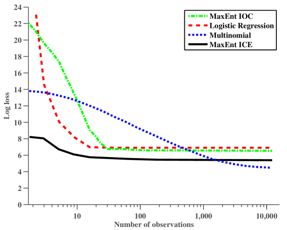
Figure 1: Prediction error (log loss) as a function of number of observations in the synthetic routing game.

In Figure 1, we see that MaxEnt ICE predicts behavior with higher accuracy than all other algorithms when the number of observations is limited. In particular, it achieves close to its best performance with only $16$ observations. The maximum likelihood estimator eventually overtakes it, as expected since it will ultimately converge to $\sigma^{\Gamma}$, but only after $10,000$ observations, or close to as many observations as there are outcomes in the game. MaxEnt ICE cannot learn the true behavior exactly in this case without additional constraints due to the social welfare criteria the true behavior optimizes. That is, our rationality assumption does not hold in this case. We note that the logistic regression classifier and the inverse optimal control techniques perform better than the multinomial under low sample sizes, but they fail to outperform MaxEnt ICE due to their inability to appreciate the strategic nature of the game.

Next, we evaluate behavior transfer from this routing game to four similar games, the results of which are displayed in Table 1. The first game, Add Highway, adds a new route to the game. That is, we simulate the city building a new highway. The second game, Add Driver, adds another driver to the game. The third game, Gas Shortage, keeps the structure of the game the same, but changes the reward function to make gas mileage more important to the drivers. The final game, Congestion, simulates adding construction to the major roadway, delaying the drivers. Here, we do not share deviations across the training and test game and we add a slack variable in the primal to ensure feasibility.

Problem	Logistic Regression	MaxEnt Ice
Add Highway	4.177	3.093
Add Driver	4.060	3.477
Gas Shortage	3.498	3.137
Congestion	3.345	2.965

Table 1: Transfer error (log loss) on unobserved games.

These transfer experiments even more directly demonstrate the benefits of learning utility weights rather than directly learning the joint-action distribution; direct strategy-learning approaches are incapable of being applied to general transfer setting. Thus, we can only compare against the Logistic Regression. We see from Table 1 that MaxEnt ICE outperforms the Logistic Regression in all of our tests. For reference, in these new games, the uniform strategy has a loss of approximately $6.8$ in all games, and the true behavior has a loss of approximately $2.7$.

These experiment demonstrates that learning underlying utility functions to estimate observed behavior can be much more data-efficient for small sample sizes. Additionally, it shows that the regret-based assumptions of MaxEnt ICE are beneficial in strategic settings, even though our rationality assumption does not hold in this case.

7.2 Market Entry Game

We next evaluate our approach against a number of baselines on data gathered for the Market Entry Prediction Competition (Erev et al., 2010). The game has four players and is repeated for fifty trials and is meant to simulate a firm’s decision to enter into a market. On each round, all four players simultaneous decide whether or not to open a business. All players who enter the market receive a stochastic payoff centered at $10-kE$, where $k$ is a fixed parameter unknown to the players and $E$ is the number of players who entered. Players who do not enter the market receive a stochastic payoff with zero mean. After each round, each player is shown their reward, as well as the reward they would have received by choosing the alternative.

Observations of human play were gathered by the CLER lab at Harvard (Erev et al., 2010). Each student involved in the experiment played ten games lasting fifty rounds each. The students were incentivized to play well through a monetary reward proportional to their cumulative utility. The parameter $k$ was randomly selected in a fashion so that the Nash equilibrium had an entry rate of $50\%$ in expectation. In total, $30,000$ observations of play were recorded. The intent of the competition was to have teams submit programs that would play in a similar fashion to the human subjects. That is, the data was used at test time to validate performance. In contrast, our experiments use actual observations of play at training time to build a predictive model of the human behavior. As we are interested in stationary behavior, we train and test on only the last twenty five trials of each game.

We compared against two baselines. The first baseline, labeled Multinomial in the figures, is a smoothed multinomial distribution trained to minimize the leave-one-out cross validation loss. This baseline does not make use of any features of the games. That is, if the players indeed play according to the Nash equilibrium we would expect this baseline to learn the uniform distribution. The second baseline, labeled Logistic Regression in the figures, simply uses regularized logistic regression to learn a linear classification boundary over the outcomes of the game using the same features presented to our method. Operationally, this is equivalent to using MaxEnt Inverse Optimal Control in a single-agent setting where the utility is summed across all the players. This baseline has similar representational power to our method, but lacks an understanding of the strategic elements of the game.

Figure 2: Test log loss using only the game’s expected utility as a feature in the market entry experiment.

In Figure 2, we see a comparison of our method against the baselines when only the game’s true expected utility is used as the only feature. We see that our method outperforms both baselines across all sample sizes. We also observe the multinomial distribution performs slightly better than the uniform distribution, which attains a log loss of $4$, though substantially worse than logistic regression and our method, indicating that the human players are not particularly well-modeled by the Nash equilibrium. Our method substantially outperforms logistic regression, indicating that there is indeed a strategic interaction that is not captured in the utility features alone.

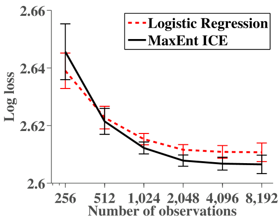
Figure 3: Test log loss using a number of history summary features in the market entry experiment.

In Figure 3, we see a comparison of our method against the baselines using a variety of predictive features. In particular, we summarize a round using the observed action frequencies, average reward, and reward variance up to that point in the round. To weigh recent observations more strongly, we also employ exponentially-weighted averages. We observe that the use of these features substantially improves the predictive power of the feature-based methods. Interestingly, we also note that the addition of these summary features also narrows the gap between logistic regression and MaxEnt ICE. Under low sample sizes, the logistic model performs the best, but our method overtakes it as more data is made available for training. It appears that in this scenario, much of the strategic behavior demonstrated by the participants can be captured by these history features.

7.3 Mid-scale Hotel Market Entry

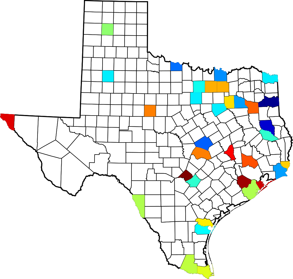
Figure 4: Regulatory index values for select counties in Texas. Blue means little regulation and lower costs to enter the market. Red means higher costs.

For our final experimental evaluation, we considered the task of predicting the behavior of mid-scale hotel chains, like Holiday Inn and Ramada, in the state of Texas. Given demographic and regulatory features of a county, we wish to predict if each chain is likely to open a new hotel or to close an existing one. The observations of play are derived from quarterly tax records over a fifteen year period from forty counties, amounting to a total of $2,205$ observations. The particular counties selected had records of all of the demographic and regulatory features, had at least four action observations, and none was a chain’s flagship county. Figure 4 highlights the selected counties and visualizes their regulatory practices.

The demographic and regulatory features were aggregated from various sources and generously provided to us by Prof. Junichi Suzuki (2010). The demographic features for each county include quantities such as size of its population and its area, employment and household income statistics, as well as the presence or absence of an interstate, airport or national park. The regulatory features are indices measuring quantities such as commercial land zoning restrictions, tax rates and building costs. In addition to these noted features, which are fixed across all time periods, there are time-varying features such as the number of hotels and rooms for each chain and the aggregate quarterly income.

We model each quarterly decision as a parameterized simultaneous-move game with six players. Each player, a mid-scale hotel chain, has the action set $\{\text{Close},\text{NoAction},\text{Open}\}$, resulting in $729$ total outcomes. For the game’s utility, we allocated the county’s features to each player in proportion to how many hotels they owned. That is, if a player operated 3 out of 10 hotels, the features associated with utility at that outcome would be the county’s feature vector scaled by $0.3$. We included bias features associated with each action to account for fixed costs associated with opening or closing a hotel.

In the observation data, there are a small number of instances where a chain opens or closes more than one hotel during a quarter. These events are mapped to Open and Close respectively. Though the outcome-space is quite large, the outcome distribution is extremely biased and the actions of the chains are highly correlated. In particular, over $80\%$ of time the time no action is taken, around $17\%$ of the time a single chain acts, and less than $3\%$ of the time more than one chain acts. As a result, one expects the featureless multinomial estimator to have reasonable performance despite a large number of classes.

For experimentation, we evaluated four algorithms: a smoothed multinomial distribution trained to minimize the leave one out cross-validation loss, MaxEnt inverse optimal control trained once for all players, multi-class logistic regression over the joint action space, and regret-matching ICE with utility matching constraints. As the resulting optimizations for the latter two algorithms are smooth, we employed the L-BFGS quasi-Newton method with L2-regularization for training (Nocedal, 1980). As a substitute for L1-regularization, we selected the $23$ best features based on their reduction in training error when using logistic regression. Each county had $63$ features available. Of the top $23$ features selected, $11$ were regulatory indices.

For the logistic regression and ICE predictors, we only used utility features on the 13 high probability outcomes (no firms build, and one firm acting). The remaining outcomes had only bias features associated with them to help prevent overfitting. We experimented with a number of types of bias features, for example, 4 bias features (one for no firms build, one for a single firm builds, one for a single firm closes and one for all remaining outcomes), as well as 729 bias features (one for each outcome). We found that, though on their own the different bias features had varied predictive performance, when combined with utility and regret features they were quite similar given the appropriate regularization. In the best performing model, which we present here, we used 729 bias features resulting in $1,028$ parameters to the logistic regression model.

In the ICE predictor, we tied together the weights for each deviation across all the players to reduce the number of model parameters. For example, all players shared the same dual parameters for the $\text{NoAction}\rightarrow\text{Open}$ deviation. Effectively, this alters the rationality assumption such that the average regret across all players is the quantity of interest, instead of the maximum regret. Operationally, this is implemented as summing each deviation’s gradient in the dual. This treats the players anonymously, thus we implicitly and incorrectly assume that conditioned on the county’s parameters each firm is identical. Due to the use parameter tying, the ICE predictor has an additional $156$ model parameters.

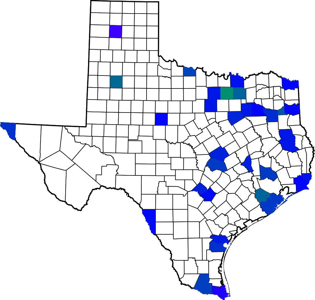
Figure 5: The marginalized probability that a chain will build a hotel in Spring 1996 predicted by MaxEnt ICE. Brighter shades of green denote higher probabilities.

The test losses reported were computed using ten-fold cross validation. To fit the regularization parameters for logistic regression, MaxEnt IOC and MaxEnt ICE, we held out $10\%$ of the training data and performed a parameter sweep. For logistic regression, a separate parameter sweep and regularization was used for the bias and utility features. For MaxEnt ICE, an additional regularization parameter was selected for the regret parameters. A sample of the predictions from MaxEnt ICE are shown in Figure 5.

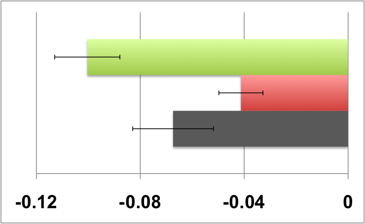
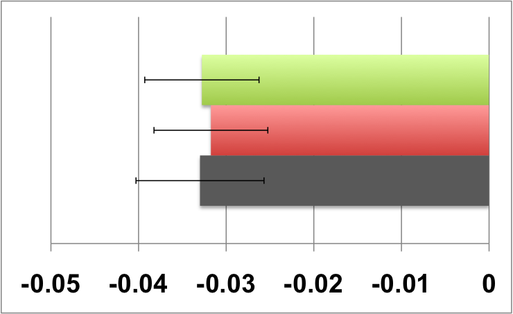
Figure 6: (Left) Test log loss on the full outcome space relative to the smoothed multinomial, which has log loss $1.58234\pm 0.058088$. (Center) Test log loss no build vs. build outcomes only. Loss is relative multinomial, with log loss $0.721466\pm 0.016539$. (Right) Test log loss conditioned on build outcomes only. Loss is relative multinomial, with log loss $6.5911\pm 0.116231$.

In the left of Figure 6, we present the test errors of the three parameterized methods in terms of their offset from that of the featureless multinomial. This quantity has lower variance than the absolute errors, allowing for more accurate comparisons. We see that the addition of the regret features more than doubles the improvement of logistic regression from $2.6\%$ to $6.3\%$, where as the inverse optimal control method only sees a $4.3\%$ improvement.

In the center of Figure 6, we show the test log-loss when the methods are only required to predict if any firm acts. Here, the models are still trained over their complete outcome spaces and their predictions are marginalized. We see that all three methods are equal within noise. That is, the differences in the predictive performances come solely from each method’s ability to predict who acts. We additionally performed this experiment without the use of regulatory features and found that the logistic regression method achieved a relative loss of $-0.027300$. Using a paired comparison between the two methods, we note that this difference of $0.004443$ is significant with error $0.001886$. This echoes Suzuki’s conclusions the regulatory environment in this industry affect firms’ decisions to build new hotels (Suzuki, 2010), measured here by improvements in predictive performance.

In the right of Figure 6, we demonstrate the test log loss conditioned on at least one firm acting—the portion of the loss that differentiates the methods. The logistic regression method with only utility features performs the worst with a $1.8\%$ improvement over the multinomial base line, the individual inverse optimal control method improves by $4.1\%$ and MaxEnt ICE performs the best with a $6.3\%$ improvement. That is, the addition of regret features, and hence accounting for the strategic aspects of the game, have a significant effect on the predictive performance in this setting. We note that replacing the regulatory features in the regret portion of the MaxEnt ICE model actually slightly improves performance to $-0.471763$, though not by a significant margin. This implies that the regulatory features have little or no bearing on predicting exactly the firm that will act, which suggests the regulatory practices are unbiased.

8 Conclusion

In this article, we develop a novel approach to behavior prediction in strategic multi-agent domains. We demonstrate that by leveraging a rationality assumption and the principle of maximum entropy our method can be efficiently implemented while achieving good statistical performance. Empirically, we displayed the effectiveness of our approach on two market entry data sets. We demonstrated both the robustness of our approach to errors in our assumption as well as the importance of considering strategic interactions.

Our future work will consider two new directions. First, we will address classes of games where the action sets and players differ. A key benefit of our current approach is that it enables these to differ between training and testing which we only leverage modestly in the transfer experiments for route prediction. This will involve investigating from a statistical point of view novel notions of a deviation and their corresponding equilibrium concepts Second, we will consider different models of interactions, such as stochastic games and extensive-form games. These models, though no more expressive than matrix games, can often represent interactions exponentially more succinctly. From a practical standpoint, this avenue of research will allow for the application of our methods to a broader class of problems, including, for instance, exploring the time series dependencies within the Texas Hotel Chain data.

Appendix

Proof of Lemma 1

Proof.

The lower bound holds as a consequence of $\Phi^{\mbox{int}}\subseteq\Phi^{\mbox{swap}}$.

$$\mbox{Since~{}}\max_{x\in A_{i},y\in A_{i}}r^{\Gamma}_{i;x\rightarrow y}(\sigma^{\Gamma}|w) \geq r^{\Gamma}_{i;x\rightarrow x}(\sigma^{\Gamma}|w)=0,$$ (49)

$$\operatorname{Regret}^{\Gamma}_{\Phi^{\mbox{swap}}}(\sigma^{\Gamma}|w) =\max_{i\in\mathcal{N}}\sum_{x\in A_{i}}\max_{y\in A_{i}}r^{\Gamma}_{i;x\rightarrow y}(\sigma^{\Gamma}|w)$$ (50)

$$\leq A\cdot\max_{i\in\mathcal{N}}\max_{x\in A_{i}}\max_{y\in A_{i}}r^{\Gamma}_{i;x\rightarrow y}(\sigma^{\Gamma}|w)$$ (51)

$$=A\cdot\operatorname{Regret}^{\Gamma}_{\Phi^{\mbox{int}}}(\sigma^{\Gamma}|w).$$ (52)

∎

Proof of Theorem 3

The proof of Theorem 3 immediately follows from the following lemma.

Lemma 4.

For any utility function $w\in\mathcal{K}$, $r^{\Gamma}_{f}(\hat{\sigma}^{\Gamma}|w)\leq\operatorname{Regret}^{\Gamma}_{\Phi_{f}}(\sigma^{\Gamma}|w)$ if and only if there exists an $\eta_{f}\in\Delta_{\Phi_{f}}$ such that $r^{\Gamma}_{f}(\hat{\sigma}^{\Gamma})-\mathbb{E}_{g\sim\eta_{f}}\left[r^{\Gamma}_{g}(\sigma^{\Gamma})\right]\in-\mathcal{K}^{*}$.

Proof.

Assume that for all $w\in\mathcal{K}$, $r^{\Gamma}_{f}(\hat{\sigma}^{\Gamma}|w)\leq\operatorname{Regret}^{\Gamma}_{\Phi_{f}}(\sigma^{\Gamma}|w)$, $\exists\eta_{f}\in\Delta_{\Phi_{f}}$ such that

$$r^{\Gamma}_{f}(\hat{\sigma}^{\Gamma}|w) \leq\mathbb{E}_{g\sim\eta_{f}}\left[r^{\Gamma}_{g}(\sigma^{\Gamma}|w)\right]$$ (53)

Since $$0\in\mathcal{K}$$,

$$\max_{w\in\mathcal{K}}r^{\Gamma}_{f}(\hat{\sigma}^{\Gamma}|w)-\mathbb{E}_{g\sim\eta_{f}}\left[r^{\Gamma}_{g}(\sigma^{\Gamma}|w)\right]\leq 0$$ (54)

$$=r^{\Gamma}_{f}(\hat{\sigma}^{\Gamma}|0)-\mathbb{E}_{g\sim\eta_{f}}\left[r^{\Gamma}_{g}(\sigma^{\Gamma}|0)\right]$$ (55)

$$=\max_{w\in\mathcal{K},t}\;\;r^{\Gamma}_{f}(\hat{\sigma}^{\Gamma}|w)-t,\;\mbox{subject to:~{}}t\geq r^{\Gamma}_{g}(\sigma^{\Gamma}|w),\;\forall g\in\Phi_{f}.$$ (56)

By Slater’s condition, strong duality holds and the resulting dual is the feasibility problem

$$=\min_{\eta_{f}\in\Delta_{\Phi_{f}}}\;\;0,\;\mbox{subject to:~{}}r^{\Gamma}_{f}(\hat{\sigma}^{\Gamma})-\mathbb{E}_{g\sim\eta_{f}}\left[r^{\Gamma}_{g}(\sigma^{\Gamma})\right]\in-\mathcal{K}^{*}.$$ (57)

Assume $$\exists\eta_{f}\in\Delta_{\Phi_{f}} y\in\mathcal{K}^{*} r^{\Gamma}_{f}(\hat{\sigma}^{\Gamma})-\mathbb{E}_{g\sim\eta_{f}}\left[r^{\Gamma}_{g}(\sigma^{\Gamma})\right]+y=0 w\in\mathcal{K}$$ and such that , then for any

$$r^{\Gamma}_{f}(\hat{\sigma}^{\Gamma}|w) -\mathbb{E}_{g\sim\eta_{f}}\left[r^{\Gamma}_{g}(\sigma^{\Gamma}|w)\right]+\langle y,w\rangle=\langle 0,w\rangle=0.$$ (58)

By the definition of the dual cone $$\langle y,w\rangle\geq 0$$, therefore

$$r^{\Gamma}_{f}(\hat{\sigma}^{\Gamma}|w) \leq\mathbb{E}_{g\sim\eta_{f}}\left[r^{\Gamma}_{g}(\sigma^{\Gamma}|w)\right]\leq\max_{g\in\Phi_{f}}{r^{\Gamma}_{g}(\sigma^{\Gamma}|w)}=\operatorname{Regret}^{\Gamma}_{\Phi_{f}}(\sigma^{\Gamma}|w).$$ (59)

∎

Proof of Theorem 4

The proof of Theorem 4 immediately follows from the following lemma.

Lemma 5.

If joint strategy $\sigma^{\Gamma}$ has $\varepsilon$ external regret, and $\Gamma$ is 2-player and constant-sum with respect to $w$, then the marginal strategies form a $2\varepsilon$-Nash equilibrium under utility function $w$.

Proof.

Denote one player $x$ and the other $y$ and their marginal strategies as $\bar{\sigma}^{\Gamma}_{x}$ and $\bar{\sigma}^{\Gamma}_{y}$ respectively. We are given

$$\forall\sigma^{\Gamma}_{x}\in\Delta_{A_{x}},\quad u^{\Gamma}_{x}(\sigma^{\Gamma}_{x},\bar{\sigma}^{\Gamma}_{y}|w)-u^{\Gamma}_{x}(\sigma^{\Gamma}|w) \leq\varepsilon\mbox{~{}and,}$$ (60)

$$\forall\sigma^{\Gamma}_{y}\in\Delta_{A_{y}},\quad u^{\Gamma}_{y}(\sigma^{\Gamma}_{y},\bar{\sigma}^{\Gamma}_{x}|w)-u^{\Gamma}_{y}(\sigma^{\Gamma}|w) \leq\varepsilon$$ (61)

as when either player deviates, the other resorts to playing his marginal strategy. Substituting $\bar{\sigma}^{\Gamma}_{y}$ for $\sigma^{\Gamma}_{y}$ and summing, we get $\forall\sigma^{\Gamma}_{x}\in\Delta_{A_{x}}$

$$u^{\Gamma}_{x}(\sigma^{\Gamma}_{x},\bar{\sigma}^{\Gamma}_{y}|w)+u^{\Gamma}_{y}(\bar{\sigma}^{\Gamma}_{y},\bar{\sigma}^{\Gamma}_{x}|w)-\left[u^{\Gamma}_{y}(\sigma^{\Gamma}|w)+u^{\Gamma}_{x}(\sigma^{\Gamma}|w)\right] \leq 2\varepsilon$$ (62)

$$u^{\Gamma}_{x}(\sigma^{\Gamma}_{x},\bar{\sigma}^{\Gamma}_{y}|w)+u^{\Gamma}_{y}(\bar{\sigma}^{\Gamma}_{y},\bar{\sigma}^{\Gamma}_{x}|w)-C \leq 2\varepsilon$$ (63)

$$u^{\Gamma}_{x}(\sigma^{\Gamma}_{x},\bar{\sigma}^{\Gamma}_{y}|w)+\left[C-u^{\Gamma}_{x}(\bar{\sigma}^{\Gamma}_{y},\bar{\sigma}^{\Gamma}_{x}|w)\right]-C \leq 2\varepsilon$$ (64)

$$u^{\Gamma}_{x}(\sigma^{\Gamma}_{x},\bar{\sigma}^{\Gamma}_{y}|w)-u^{\Gamma}_{x}(\bar{\sigma}^{\Gamma}_{y},\bar{\sigma}^{\Gamma}_{x}|w) \leq 2\varepsilon$$ (65)

A symmetric argument shows the equivalent statement for the opposing player. ∎

Proof of Theorem 7

Proof.

The Legrange dual function,

$$L(\theta,\alpha,\beta,u,v,x)=\;\;\max_{\hat{\sigma}^{\Gamma},\eta,y} -\sum_{a\in\mathcal{A}}\hat{\sigma}^{\Gamma}(a)\log\hat{\sigma}^{\Gamma}(a)+$$ (66)

$$\sum_{f\in\Phi}\alpha_{f}\left(1-\sum_{g\in\Phi}\eta_{f}(g)\right)+\beta\left(1-\sum_{a\in\mathcal{A}}\hat{\sigma}^{\Gamma}(a)\right)+$$ (67)

$$\sum_{f\in\Phi}\langle r^{\Gamma}_{f}(\hat{\sigma}^{\Gamma})-\sum_{f,g\in\Phi}\eta_{f}(g)r^{\Gamma}_{g}(\sigma^{\Gamma})+y_{f},\theta_{f}\rangle+$$ (68)

$$\sum_{f\in\Phi}v_{f}\cdot\eta_{f}+u\cdot\hat{\sigma}^{\Gamma}+\langle y_{f},x_{f}\rangle,$$ (69)

is an upper bound on the primal objective for all $u,v\geq 0$ and $x\in\mathcal{K}^{**}$. We solve the unconstrained maximization by setting the derivatives with respect to $\hat{\sigma}^{\Gamma},\eta,y$ to zero,

$$\log\hat{\sigma}^{\Gamma}(a) =u(a)-1-\beta-\sum_{f\in\Phi}\langle r^{\Gamma}_{f}(a),\theta_{f}\rangle$$ (70)

$$\langle r^{\Gamma}_{g}(\sigma^{\Gamma}),\theta_{f}\rangle-\alpha_{f}+v_{f}(g) =0 \forall f,g\in\Phi$$ (71)

$$\theta_{f} =-x_{f}. \forall f\in\Phi$$ (72)

Substituting this solution back into the Legrangian and minimizing this upper bound gives

$$\min_{\theta\in\mathcal{K}^{**},\beta} \;\;\exp(-1-\beta)Z^{\Gamma}(\theta)+\sum_{f\in\Phi}\alpha_{f}+\beta\quad\mbox{subject to:}$$ (73)

$$\langle r^{\Gamma}_{g}(\sigma^{\Gamma}),\theta_{f}\rangle\leq\alpha^{f}. \forall f,g\in\Phi$$ (74)

Solving for $\beta$ explicitly we get $\beta=\log Z^{\Gamma}(\theta)-1$, and moving the constraint into the objective gives our result:

$$\min_{\theta\in\mathcal{K}^{**}} \;\;\sum_{f\in\Phi}\operatorname{Regret}^{\Gamma}_{\Phi}(\sigma^{\Gamma}|\theta_{f})+\log Z^{\Gamma}(\theta).$$ (75)

∎

Proof of Theorem 9

Proof.

Let $\{e_{1},e_{2},\ldots,e_{K}\}$ be an orthonormal basis for $V$, where $K=\dim{V}$. We first bound how well the regrets match in each basis direction.

$$P\Big{[}\max_{f\in\Phi,k\in[K]}|r^{\tilde{\xi}}_{f}(\tilde{\sigma}|e_{k})-r^{\xi}_{f}(\sigma|e_{k})|\geq\epsilon\Delta\Big{]} \leq P\Big{[}\bigcup_{f\in\Phi,k\in[K]}\big{(}|r^{\tilde{\xi}}_{f}(\tilde{\sigma}|e_{k})-r^{\xi}_{f}(\sigma|e_{k})|\geq\epsilon\Delta\big{)}\Big{]}$$ (76)

$$\leq\sum_{f\in\Phi,k\in[K]}P\Big{[}|r^{\tilde{\xi}}_{f}(\tilde{\sigma}|e_{k})-r^{\xi}_{f}(\sigma|e_{k})|\geq\epsilon\Delta\Big{]}$$ (77)

$$\leq 2|\Phi|K\exp\left(-2T\epsilon^{2}\right)\leq\delta.$$ (78)

$$T \geq\frac{1}{2\epsilon^{2}}\log\frac{2|\Phi|\dim{V}}{\delta}.$$ (79)

Next, we bound how well the regrets match under $$w$$, given all regrets are close.

$$|r^{\tilde{\xi}}_{f}(\tilde{\sigma}|w)-r^{\xi}_{f}(\sigma|w)| =|\sum_{k=1}^{K}\alpha_{k}r^{\tilde{\xi}}_{f}(\tilde{\sigma}|e_{k})-\alpha_{k}r^{\xi}_{f}(\sigma|e_{k})|$$ (80)

$$\leq\sum_{k=1}^{K}|\alpha_{k}||r^{\tilde{\xi}}_{f}(\tilde{\sigma}|e_{k})-r^{\xi}_{f}(\sigma|e_{k})|$$ (81)

$$\leq\epsilon\Delta\sum_{k=1}^{K}|\alpha_{k}|$$ (82)

$$\leq\epsilon\Delta\|w\|_{1}.$$ (83)

∎

Proof of Theorem 10

Proof.

Unlike Theorem 9, we will bound the error of regrets directly.

$$P\Big{[}\max_{f\in\Phi}r^{\tilde{\xi}}_{f}(\tilde{\sigma}|w)-r^{\xi}_{f}(\sigma|w)\geq\epsilon\Delta(w)\Big{]} \leq P\Big{[}\bigcup_{f\in\Phi}\big{(}r^{\tilde{\xi}}_{f}(\tilde{\sigma}|w)-r^{\xi}_{f}(\sigma|w)\geq\epsilon\Delta(w)\big{)}\Big{]}$$ (84)

$$\leq\sum_{f\in\Phi}P\Big{[}r^{\tilde{\xi}}_{f}(\tilde{\sigma}|w)-r^{\xi}_{f}(\sigma|w)\geq\epsilon\Delta(w)\Big{]}$$ (85)

$$\leq 2|\Phi|\exp\left(-2T\epsilon^{2}\right)\leq\delta$$ (86)

$$T \geq\frac{1}{2\epsilon^{2}}\log\frac{|\Phi|}{\delta}.$$ (87)

∎

References

- Abbeel and Ng [2004] P. Abbeel and A. Y. Ng. Apprenticeship learning via inverse reinforcement learning. In Proceedings of the International Conference on Machine Learning, 2004.
- Berry et al. [1995] S. Berry, J. Levinsohn, and A. Pakes. Automobile prices in market equilibrium. Econometrica, 63(4):841–890, July 1995.
- Blum and Mansour [2007] A. Blum and Y. Mansour. Algorithmic Game Theory, chapter Learning, Regret Minimization and Equilibria, pages 79–102. Cambridge University Press, 2007.
- Camerer and Ho [1999] C. Camerer and T. H. Ho. Experience weighted attraction learning in normal form games. Econometrica, 67:827––874, 1999.
- Conlin and Kadiyali [2006] M. Conlin and V. Kadiyali. Entry-deterring capacity in the texas lodging industry. Journal of Economics and Management Strategy, pages 167–185, 2006.
- Della Pietra et al. [2002] S. Della Pietra, V. Della Pietra, and J. Lafferty. Inducing features of random fields. IEEE Transactions on Pattern Analysis and Machine Intelligence, 19(4):380–393, 2002. ISSN 0162-8828.
- Dudík et al. [2007] M. Dudík, S. J. Phillips, and R. E. Schapire. Maximum entropy density estimation with generalized regularization and an application to species distribution modeling. Journal of Machine Learning Research, 8:1217–1260, 2007.
- Erev and Barron [2005] I. Erev and G. Barron. On adaptation, maximization and reinforcement learning among cognitive strategies. Psychological Review, 112:912–931, 2005.
- Erev et al. [2008] I. Erev, E. Ert, and E. Yechiam. Loss aversion, diminishing sensitivity, and the effect of experience on repeated decisions. Journal of Behavioral Decision Making, 21:575–597, 2008.
- Erev et al. [2010] I. Erev, E. Ert, and A. E. Roth. A choice prediction competition for market entry games: An introduction. Games, 1:117–136, 2010.
- Foster and Vohra [1996] D. Foster and R. Vohra. Calibrated learning and correlated equilibrium. Games and Economic Behavior, 21:40–55, 1996.
- Grünwald and Dawid [2003] P. D. Grünwald and A. P. Dawid. Game theory, maximum entropy, minimum discrepancy, and robust bayesian decision theory. Annals of Statistics, 32:1367–1433, 2003.
- Hart and Mas-Colell [2000] S. Hart and A. Mas-Colell. A simple adaptive procedure leading to correlated equilibrium. Econometrica, 68(5):1127–1250, 2000.
- Henry et al. [2010] P. Henry, C. Vollmer, B. Ferris, and D. Fox. Learning to navigate through crowded environments. In Proceedings of Robotics and Automation, 2010.
- Jaynes [1957] E. T. Jaynes. Information theory and statistical mechanics. Physical Review, 106(4):620–630, May 1957.
- Kakade et al. [2003] S. Kakade, M. Kearns, J. Langford, and L. Ortiz. Correlated equilibria in graphical games. In Proceedings of Electronic Commerce, pages 42–47, 2003.
- McFadden [1974] D. McFadden. The measurement of urban travel demand. Journal of Public Economics, 3(4):303–328, 1974.
- McKelvey and Palfrey [1995] R. McKelvey and T. Palfrey. Quantal response equilibria for normal form games. Games and Economic Behavior, 10:6––38, 1995.
- Myers and Sadler [1960] J. Myers and E. Sadler. Effects of range of payoffs as a variable in risk taking. Journal of Experimental Psychology, 60:306–309, 1960.
- Nevo [2001] A. Nevo. Measuring market power in the ready-to-eat cereal industry. Econometrica, 69(2):307–342, March 2001.
- Ng and Russell [2000] A. Ng and S. Russell. Algorithms for inverse reinforcement learning. In Proceedings of the International Conference on Machine Learning, 2000.
- Nocedal [1980] J. Nocedal. Updating quasi-newton matrices with limited storage. Mathematics of Computation, 35(151):773––782, 1980.
- Ortiz et al. [2007] L. E. Ortiz, R. E. Shapire, and S. M. Kakade. Maximum entropy correlated equilibrium. In Proceedings of Artificial Intelligence and Statistics, pages 347–354, 2007.
- Osborne and Rubinstein [1994] M. Osborne and A. Rubinstein. A course in game theory. The MIT press, 1994. ISBN 0262650401.
- Petrin [2002] A. Petrin. Quantifying the benefits of new products: The case of the minivan. Journal of Political Economy, 110(4), 2002.
- Ratliff et al. [2006] N. Ratliff, J. A. Bagnell, and M. Zinkevich. Maximum margin planning. In Proceedings of the International Conference on Machine Learning, 2006.
- Ratliff et al. [2009] N. D. Ratliff, D. Silver, and J. A. Bagnell. Learning to search: Functional gradient techniques for imitation learning. Autonomous Robots, 27(1):25–53, 2009.
- Shor [1985] N. Z. Shor. Minimization methods for non-differentiable functions. Springer-Verlag New York, Inc., 1985. ISBN 0-387-12763-1.
- Silver et al. [2010] D. Silver, J. A. Bagnell, and A. Stentz. Learning from demonstration for autonomous navigation in complex unstructured terrain. International Journal of Robotics Research, 29(1):1565 – 1592, October 2010.
- Suzuki [2010] J. Suzuki. Land use regulation as a barrier to entry: Evidence from the texas lodging industry. International Economic Review, 2010.
- Waugh et al. [2011a] K. Waugh, B. D. Ziebart, and J. A. Bagnell. Computational rationalization: The inverse equilibrium problem. In Proceedings of the 28th International Conference on Machine Learning, 2011a.
- Waugh et al. [2011b] K. Waugh, B. D. Ziebart, and J. A. Bagnell. Computational rationalization: The inverse equilibrium problem. arXiv, abs/1103.5254, 2011b.
- Ziebart et al. [2008a] B. D. Ziebart, A. Maas, J. A. Bagnell, and A. Dey. Maximum entropy inverse reinforcement learning. In Proceeding of the AAAI Conference on Artificial Intelligence, 2008a.
- Ziebart et al. [2008b] B. D. Ziebart, A. Maas, A. K. Dey, and J. A. Bagnell. Navigate like a cabbie: Probabilistic reasoning from observed context-aware behavior. In Proceedings of the International Conference on Ubiquitous Computing, 2008b.
- Ziebart et al. [2010] B. D. Ziebart, J. A. Bagnell, and A. K. Dey. Modeling interaction via the principle of maximum causal entropy. In Proceedings of the International Conference on Machine Learning, 2010.
- Ziebart et al. [2012] B. D. Ziebart, A. K. Dey, and J. A. Bagnell. Probabilistic pointing target prediction via inverse optimal control. In Proceedings of the International Conference on Intelligent User Interfaces, 2012.