The Chemical Composition of Praesepe (M44)
Abstract
Star clusters have long been used to illuminate both stellar evolution and Galactic evolution. They also hold clues to the chemical and nucleosynthetic processes throughout the history of the Galaxy. We have taken high signal-to-noise, high-resolution spectra of 11 solar-type stars in the Praesepe open cluster to determine the chemical abundances of 16 elements: Li, C, O, Na, Mg, Al, Si, Ca, Sc, Ti, V, Cr, Fe, Ni, Y, and Ba. We have determined Fe from Fe I and Fe II lines and find [Fe/H] = +0.12 0.04. We find that Li decreases with temperature due to increasing Li depletion in cooler stars; it matches the Li-temperature pattern found in the Hyades. The [C/Fe] and [O/Fe] abundances are below solar and lower than the field star samples due to the younger age of Praesepe (0.7 Gyr) than the field stars. The alpha-elements, Mg, Si, Ca, and Ti, have solar ratios with respect to Fe, and are also lower than the field star samples. The Fe-peak elements, Cr and Ni, track Fe and have solar values. The neutron capture element [Y/Fe] is found to be solar, but [Ba/Fe] is enhanced relative to solar and to the field stars. Three Praesepe giants were studied by Carrera and Pancino; they are apparently enhanced in Na, Mg, and Ba relative to the Praesepe dwarfs. The Na enhancement may indicate proton-capture nucleosynthesis in the Ne Na cycling with dredge-up into the atmospheres of the red giants.
1 INTRODUCTION
Open clusters have provided important information in the study of stellar evolution, Galactic chemical evolution, nucleosynthesis and light element abundances. The stars in a given cluster are formed from the pre-cluster gas with similar compositions and ages.
The Praesepe cluster is about the same age as the Hyades cluster at 0.7 Gyr (e.g. Salaris et al. 2004). Metallicity determinations cover a range of values. Boesgaard (1989) determined [Fe/H] for several open clusters using sharp-lined cluster stars with the best high-resolution spectra for each cluster; for Praesepe she used the Palomar 5-m telescope and derived [Fe/H] = +0.09 0.07. Friel & Boesgaard (1992) found [Fe/H] = +0.04 0.04 from six sharp-lined F dwarfs observed with CFHT high-resolution, high signal-to-noise spectra. With high-resolution spectra of four G dwarfs in Praesepe An et al. (2007) derived [Fe/H] = +0.11 0.03. With spectra from VLT + UVES Pace et al. (2008) found abundances for 6 elements in 7 Praesepe dwarf stars; their Fe abundances are supersolar at +0.27 0.10. The compilation of Gratton (2000) gives +0.04 0.06 and Salaris et al. (2004) use +0.13 0.06 for Praesepe as one of their calibrating clusters. Carrera & Pancino (2009) found [Fe/H] = +0.16 0.05 for three red giant stars in Praesepe.
The Hyades and Praesepe clusters have long been thought to be so similar as to be coeval having formed in the same giant molecular cloud complex. In their study of the places of origin of 24 open clusters, Palous et al. (1977) find that for the angular rotational speeds of 13.5, 15.0, 17.5 and 20.0 km s-1 kpc-1 Hyades and Praesepe were formed near each other. Their metallicities are similar at [Fe/H] +0.13, their ages are similar at 0.7 Gyr (e.g. Salaris et al. 2004, Magrini et al. 2009) and their kinematic properties are similar (Eggen 1992).
There are some intriguing differences. The activity level in Praesepe is lower than that in the Hyades. ROSAT studies of the Hyades showed a detection rate of 90% for the G dwarfs in the Hyades (Stern et al. 1995), but only 33% in the Praesepe G dwarfs (Randich & Schmidt 1995). The dichotomy in the X-ray luminosity functions is not due to membership problems, sensitivity issues or differences in rotational velocity distributions (Barrado y Navascues et al. 1998). Holland et al. (2000) and Franciosini et al. (2003) suggest that Praesepe may actually be two merging clusters of different ages. The former authors describe the main cluster with 630 M⊙ extending to 12.1 pc with a subcluster of 30 M⊙ that is 3 pc away from the center. There might be a possibility of somewhat different Fe abundances in the two merging pieces, but the major part is dominant by a factor of 21 in mass.
In this paper we present the abundances of 16 elments in 11 solar-temperature dwarfs in Praesepe from high-resolution, high signal-to-noise spectra obtained at the Keck I telescope with HIRES. We compare our results with those of Carrera & Pancino (2011) who have determined chemical abundances in three red giants in Praesepe.
2 OBSERVATIONS AND DATA REDUCTION
The stars selected for this work are main sequence stars with colors and temperatures surrounding the solar value of 5774 K. High-resolution spectra were obtained with HIRES (Vogt et al. 1994) on the Keck I telescope on Mauna Kea on two clear nights in January and February 2003. The spectral resolution is 45,000 and the signal-to-noise ratios (S/N) range from 93 to 166 with a median of 153. Typical integration times were 20 - 25 minutes. The details of the observations of 11 Praesepe stars are given in Table 1. The spectral coverage is from 5730 Å to 8140 Å with some interorder gaps. On the night of 2003 January 11 (UT) we also took a 10 s exposure of the Moon to be used as a surrogate for the solar spectrum.
Each night we obtained 13 flatfield frames and 13 bias frames as well as Th-Ar spectra at the beginning and end of the night for wavelength calibration. The data reduction was done using standard IRAF111IRAF is distributed by the National Optical Astronomical Observatories, which are operated by AURA, Inc. under contract to the NSF. routines. These include overscan-subtraction, bias-subtraction, master nightly flat-field normalizations, wavelength calibrations, scattered-light removal, cosmic ray removal, and continuum fitting. We were able to extract 19 orders of spectra.
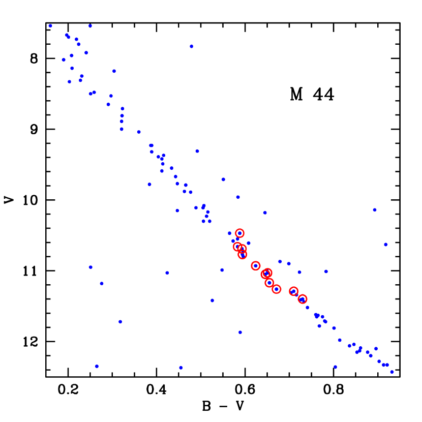
In Figure 1 we show the color-magnitude diagram for Praesepe from UBV photometry done by Johnson (1952) and Mendoza (1967). The stars we observed in Table 1 are indicated by the open circles. All of our stars are confirmed members based on radial velocity measurements of Mermilliod & Mayor (1999). All the stars are confirmed members (at 97-99%) from proper motion measurements of Jones & Cudworth (1983) and Jones & Stauffer (1991), except KW 30 which they did not measure.
Figure 2 shows 60 Å of spectrum for three of our stars which span a range in temperature. Several Fe I lines used in the analysis are indicated. The high quality of our data can be seen in this figure. It is easy to see that as the temperature decreases, the Fe I lines strength increases. Figure 3 shows the region near the Li I line for the same three stars. The Li I line decreases in strength going to cooler temperatures due to increasing depletion of Li. The three Fe I lines in that figure increase in strength with decreasing temperature. Figure 4 shows the region where the high excitation C I lines occur while Figure 5 is of the high excitation lines of the O I triplet in the same three stars.
3 ABUNDANCES
We have used both IRAF and MOOG222http://www.as.utexas.edu/ chris/moog.html (Sneden 1973, as revised in 2002) to analyze the reduced spectra. Equivalent widths were measured with the splot task in IRAF for each star. The line list we used is given in the Appendix. We edited the Fe I and Fe II line lists to omit lines weaker than 5 mÅ that might have poorer quality measurements. Most of the line lists for Fe and the other elements are from Stephens (1999), Stephens & Boesgaard (2002), Reddy et al. (2003), Kurucz (1995) and the NIST data site. Additions to those lists are described in the relevant parts of 4.
3.1 Stellar Parameter Determination
We have used the infra-red flux method (IRFM) to find . Table 2 gives the measured colors for our stars, primarily from 2MASS. Table 3 gives the temperatures derived from the color indices and the calibration of Casagrande et al. (2010).
With the exception of Sc II and Ba II, our abundances are not very sensitive to the value of log g. Inasmuch as we are dealing with stars in a cluster, we have used the relationship between log g and B-V compiled by Gray (1976) from 45 main-sequence eclipsing-binary stars. We have used the empirical relationship for microturbulent velocity derived by Edvardsson et al. (1993) with its dependency on log g and .
We determined values for [Fe/H] from 50-55 lines of Fe I and 5-6 lines of Fe II. We found the mean [Fe/H] by weighing Fe I and the Fe II results by the number of lines measured for each. In Table 4 we show these results for [FeI/H] and [FeII/H] along with the average deviation from the individual lines for each star. The final [Fe/H] was +0.117 0.039. In the subsequent models for all the stars we used [Fe/H] = 0.12. Table 5 gives the adopted model parameters for the 11 stars in this study.
3.2 Abundance Determinations
We used Kurucz (1993) model atmospheres and interpolated among his grid models to create a model atmosphere for each star. For Li we used the synth driver in MOOG to make synthetic spectra to determine the Li abundance. For the other elements we used measurements of equivalent widths and the abfind driver in MOOG, with the exception of Ba II for which we include the hyperfine splitting (hfs) and use the blends driver. (The Appendix contains a table giving the wavelengths, excitation potentials, log gf values and measured equivalent widths of the lines used for the three stars shown in Figures 2 – 5.) The final abundances are given in Table 6.
3.3 Abundance Uncertainties
We estimated errors due to uncertainties in the stellar parameters. Table 3 shows the agreement among the temperatures determined from the various color indices. The uncertainty in the mean ranges from 29 to 111 K with a mean of 56 K, median of 50 K. We chose 75 K as a conservative estimate of the uncertainty in . The average deviation from the linear relation from Gray between log g and B-V is 0.09 dex. Our choice of 0.20 dex for the uncertainty in log g is also conservative. Our mean [Fe/H] of 0.117 has a standard deviation of 0.039, so our use of 0.10 in [Fe/H] is again conservative. The Edvardsson et al. (1993) relation for microturbulent velocity has an rms scatter of 0.3 km s-1 based on 157 field stars; for cluster stars of virtually the same log g (4.38 - 4.43) the rms scatter is considerably less and we used 0.20 km s-1. Table 7 shows those abundance errors for Fe I. We added the errors in quadrature to estimate the total error due to the parameter uncertainties. In Table 8 we show the errors for the three representative stars shown in Figures 2-5 for the other elements.
4 RESULTS
4.1 Iron
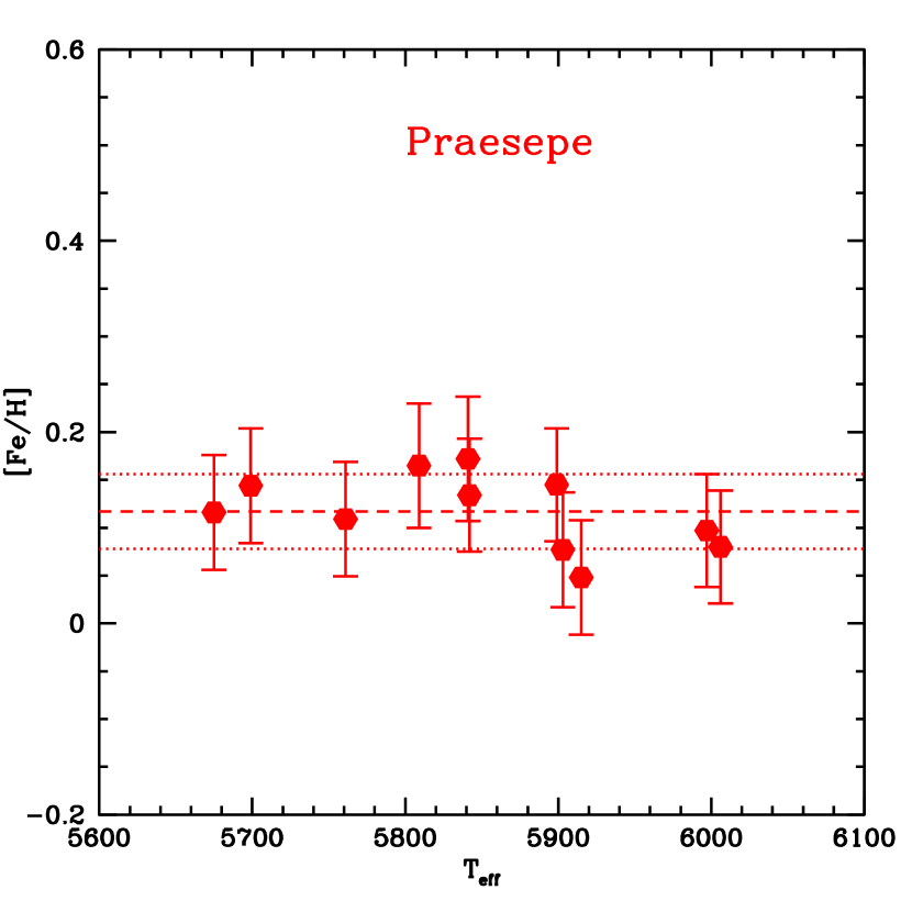
The values for [Fe/H] were given in Table 4. These are plotted in Figure 6 where the errorbars shown are due to the parameter uncertainties for each star from Table 7. We have derived the values of [Fe/H] = +0.117 0.039 (the sample standard deviation). Including the fact that there are 11 stars in our sample, the error is 0.012.
Our value for [Fe/H] of +0.12 is in good agreement with that of An et al. (2007) who found [Fe/H] = +0.11 0.03 from four G dwarfs; there are two stars in common with this study, KW 23 and KW 58, which agree better than within the quoted errors. We do not agree with Pace et al. (2008) whose [Fe/H] abundance from seven stars was supersolar at +0.27 0.10. Salaris et al. (2004) used +0.13 for [Fe/H] and Carrera & Pancino (2011) found +0.16 0.05 from three giants stars in Praesepe.
4.2 Lithium
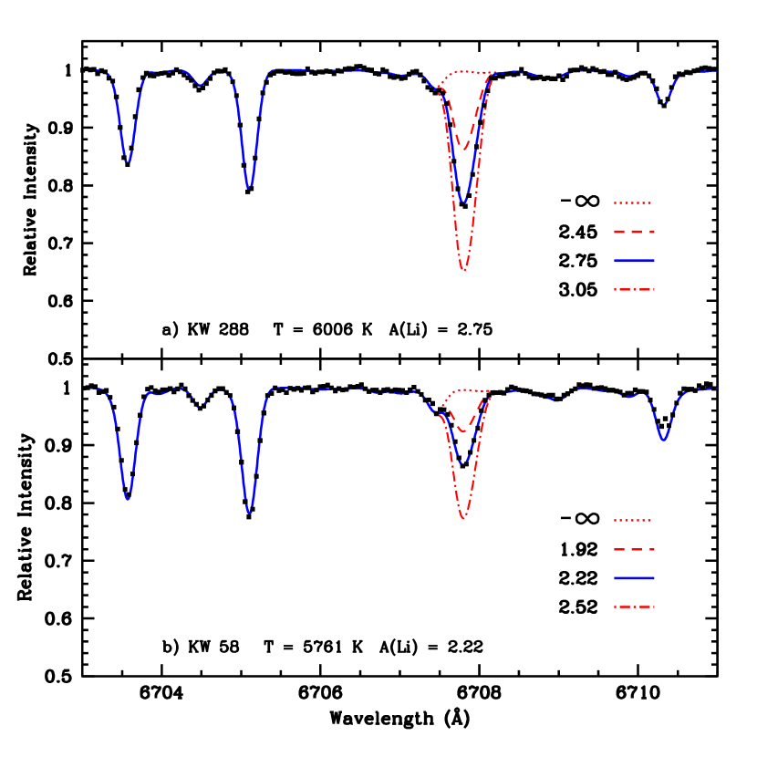
We have used MOOG with the synth driver to find Li abundances, A(Li) = log N(Li) +12.00. The line list used for the Li synthesis is from King & Hiltgen (1996). Figure 7 shows the abundance matches for two of our stars. For all 11 stars the syntheses were excellent fits to the data. Lithium abundances or upper limits have been determined by Soderblom et al. (1993) for 63 Praesepe stars with temperatures between 4970 and 6810 K from Li equivalent width measurements; these have been redetermined by them in Soderblom et al. (1995). Boesgaard & Budge (1988) found Li abundances in seven additional Praesepe F dwarfs. In 1995 Balachandran recalibrated the temperature scale and excluded photometric binaries and double-lined spectroscopic binaries from those samples leaving 59 stars. Our synthesized spectral results agree well with those that Balachandran (1995) reexamined via equivalent width measurements. The mean difference in A(Li) is +0.07 dex and those differences are result from the temperature differences. Similarly, the agreement with the Soderblom et al. revised Li abundances is good with the mean difference in A(Li) = +0.04. We have six stars in common with King & Hiltgen (1996) where our mean A(Li) difference is +0.05.
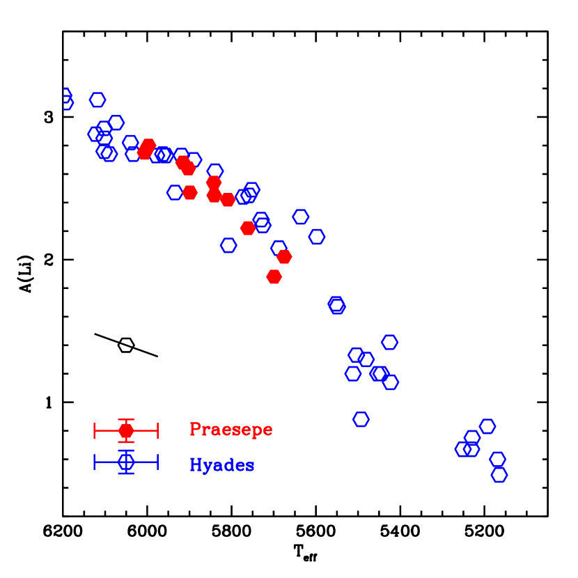
Soderblom et al. (1993, 1995) found that the low mass stars in the Praesepe cluster had higher Li abundances than the low mass stars in the Hyades with Teff 5800 K. Once Balachandran (1995) put the two clusters on the same temperature scale, that Li abundance difference disappeared. We show in our Figure 8 that Hyades and Praesepe have virtually the same Li abundances in the temperature range of our Praesepe observations: 5650 - 6000 K. Our Hyades Li abundances are taken from Boesgaard et al. (in preparation) re-evaluation of the Hyades Li abundances with the stellar parameters determined from the new Hipparcos calibration.
4.3 Carbon and Oxygen
Both C and O are formed from massive stars (10M⊙) and – through core-collapse supernovae – have enriched the gas out of which the early generations of stars were formed. These, in turn, have added their own contributions to successive generations. The bulk of the Fe is formed in intermediate mass stars in supernovae type Ia, so the production of Fe lags behind that of C and O, e.g. Tinsley (1980), Wheeler et al. (1989). This leads to the expectation that [C/Fe] and [O/Fe] will be greater than zero in metal-poor stars. A recent study that included both Fe and O in 117 stars with [Fe/H] from 0.5 to 3.5 by Boesgaard et al. (2011) shows a monotonic decrease in [O/Fe] with [Fe/H]. At [Fe/H] = 3.5 the value for [O/Fe] is +1.0 and by [Fe/H] = 0.5 the value for [O/Fe] has declined to +0.2. A similar trend was found by Boesgaard et al. (1999) and Israelian et al. (1998, 2001).
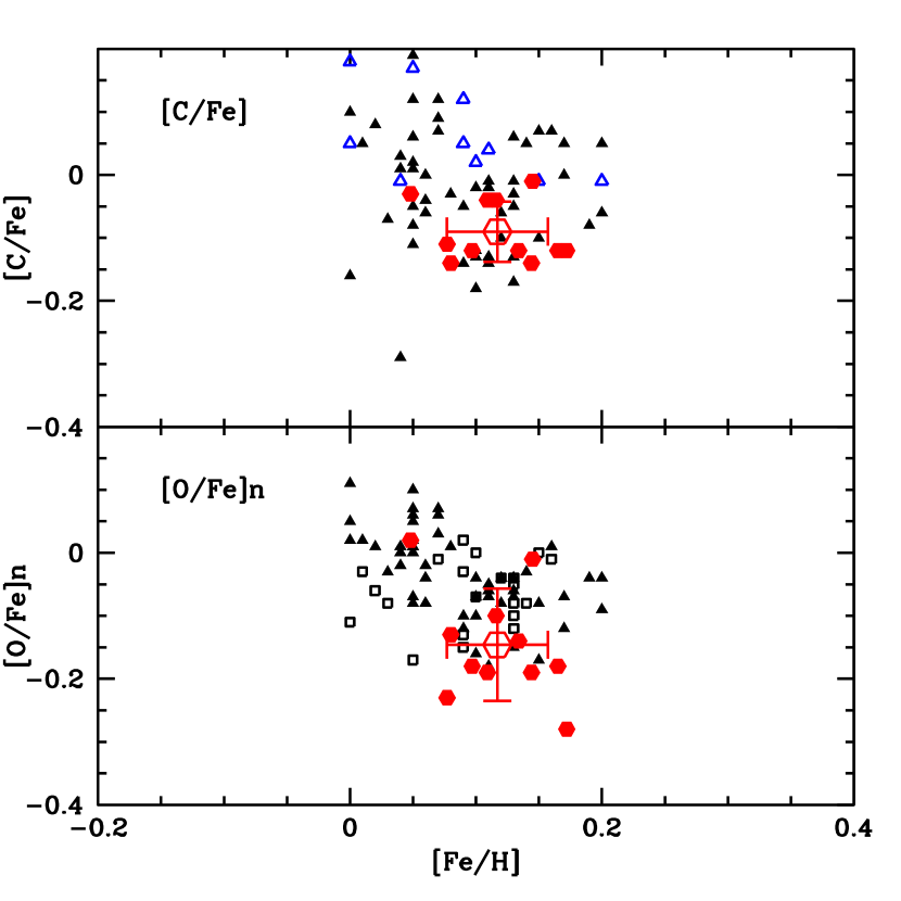
The seven lines of C I and three lines of O I (the O triplet) are all lines with high excitation potential. The gf values for C I are from Weise et al. (1996) and Reddy et al. (2003) while the O I triplet line gf values are from Weise et al. (1996). The C and O abundances in our Praesepe dwarfs are given in Table 6. The O abundances given there have been corrected for NLTE effects through the calculations of Takeda (2003). Rentzsch-Holm (1996) has studied the NLTE abundance corrections for C in stars with temperatures 7000 – 12,000 K, log g values of 3.5, 4.0, 4.5 and metallicities of [M/H] of 0.5, 0.0, +0.5, and +1.0. These trends indicate that for our solar-temperature stars with C I equivalent widths of 10 – 32 mÅ, the NLTE effects are insignificant. We can compare our C and O abundances with those in field stars. We have selected the field stars from Edvardsson et al. (1993) for O comparisons and those in Takeda & Honda (2005) for C and O. In both comparison samples we have restricted the range in [Fe/H] to be 0.00 to +0.20, enveloping our Praesepe range of +0.05 to +0.17. In addition we have used the results from Reddy et al. (2003, 2006) for C in F and G dwarfs in the thin disk and the thin-thick disk in our metallicity and temperature range. None of the comparison stars is as young as Praesepe.
Figure 9 shows the ratio [C/Fe] for the Praesepe stars in the top panel along with the Reddy et al. (2003, 2006) and Takeda & Honda (2005) comparisons. By the solar age the excess of C over Fe is expected to have disappeared. In the young Praesepe cluster (age 0.7 Gyr) the value we find for [C/Fe] of 0.14 0.07 could indicate the continued decrease in [C/Fe] with time.
The lower panel of Figure 9 shows [O/Fe] as corrected for NLTE effects for Praesepe and the two comparison samples of Edvardsson et al. (1993) and Takeda & Honda (2005). (Edvardsson et al. (1993) did not do a correction for NLTE effects, but rather calibrated their abundances found from the O I triplet alone to the abundances found in those stars where they had results from both the [O I] line at 6300 Å and the O I triplet.) As is the case for [C/Fe], we find that O has decreased relative to Fe and the mean value of [O/Fe] is 0.15 0.09. The cluster stars have O abundances typically below the field star sample.
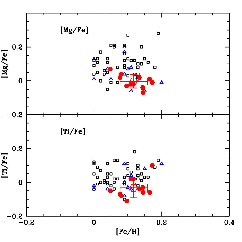
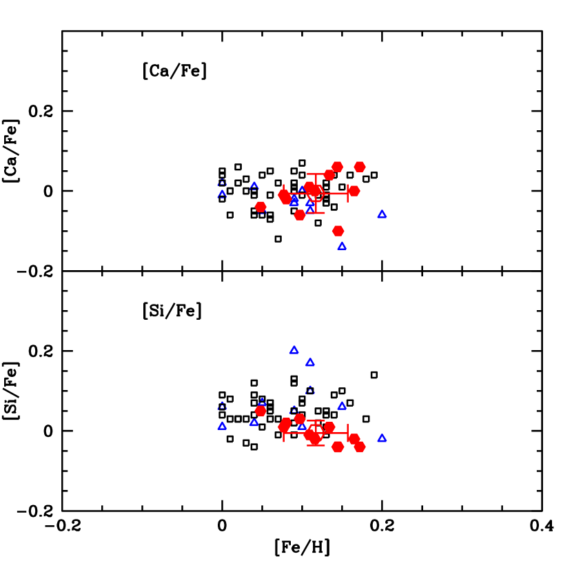
4.4 Alpha-Elements: Mg, Si, Ca, Ti
For the abundance determinations we have used two lines of Mg I, 11 lines of Si I, 10 lines of Ca I, and 11 lines of Ti I as listed in the Appendix. The alpha-element abundances are given for each star in Table 6. Their ratios normalized to Fe are shown in Figures 10 and 11 along with the mean values for [X/Fe] and [Fe/H] for Praesepe. The comparison samples are from Edvardsson et al. (1993) and Reddy et al. (2003, 2006). The field stars, except for Ca, show a larger range in abundance than do the Praesepe stars. And the Praesepe stars, again except for Ca, have lower values of [X/Fe] than the field stars. The alpha-element abundances relative to Fe (relative to solar) tend to decrease with age reaching solar at the age of the Sun. The Praesepe stars are all younger than the field star sample and do show solar abundances. The alpha ratios relative to Fe are all close to solar: [Mg/Fe] = 0.003 0.040; [Ti/Fe] = 0.035 0.062; [Ca/Fe] = 0.006 0.049; [Si/Fe] = 0.005 0.031. The mean ratio, [/Fe], is 0.012 0.015.
According to Tsujimoto et al. (1995) the contribution of SNe Ia to the solar abundances is only 1% for Mg, 25% for Ca, and 17% for Si. With the exception of Mg, both SNe Ia and SN II have contributed to the alpha-elements in the Praesepe cluster.
4.5 Fe-Peak Elements: Cr and Ni
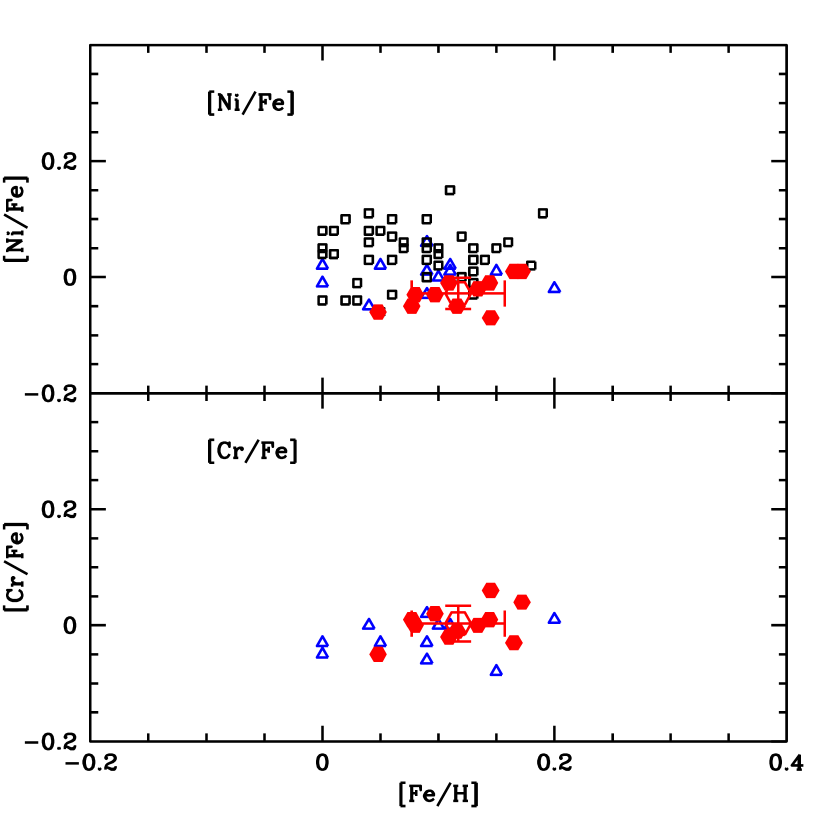
In addition to the 55 lines of Fe I and six lines of Fe II, we have measured nine lines of Cr I and 26 lines of Ni I. Abundances for Cr and Ni are given in Table 6 for each star along with the mean abundances relative to Fe and the standard deviation of the mean. Figure 12 shows the results as a function of [Fe/H] with the comparison samples of field stars. Bergemann & Cescutti (2010) studied the effects of NLTE on Cr I in the Sun and metal-poor stars. Our Cr abundances have been corrected for the overionization effect on Cr I using the solar value of log (Cr II)⊙ = 5.77 from Sobeck et al. (2007). The Praesepe cluster mean, [Cr/Fe] = 0.003 0.031, is the solar value and in agreement with the field star sample. According to Clayton (2003) both SN II and SN Ia produce Cr/Fe ratios that are roughly solar.
The mean value we find for [Ni/Fe] is also similar to the solar value at 0.028 0.027. The abundances are comparable to the field stars from Reddy et al. (2003, 2006), but seem lower than the bulk of the Edvardsson et al. (1993) field stars of comparable metallicity. Our two iron-peak elements behave as Fe does.
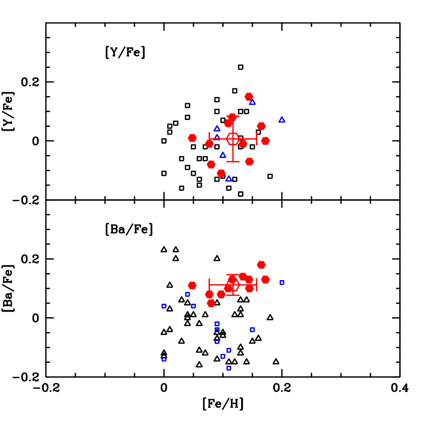
4.6 n-Capture Elements: Y and Ba
We have determined abundances for the two n-capture elements, Y and Ba, which are dominated by the s-process at different s-process peaks. For Y we have measured two lines of Y I and three lines of Y II, but not all lines were measurable in most of the stars; we also measured these lines in our lunar spectrum. The gf values for Y II are from Hannaford et al. (1982). We then normalized our stellar Y abundance to our lunar/solar Y to get [Y/H] for the Praesepe stars. For Ba we had one line of Ba II at 5853.7 Å for which we included the hyperfine structure in our analysis. The results for [Y/Fe] and [Ba/Fe] are given in Table 6. Figure 13 shows the results for [Y/Fe] (upper panel) and [Ba/Fe] (lower panel) with the field star comparison samples. The field stars show a large range (0.20) in both elements; our [Y/Fe] vales are solar near the middle of the comparison stars. Our [Ba/Fe] are somewhat higher than solar at +0.11 0.04 and near the top of the field star results. This is consistent with the results of D’Orazi et al. (2009) who found that [Ba/Fe] increases in open clusters with younger ages. They suggest that the enhancement of [Ba/Fe] would come from low mass stars (1.5M⊙).
4.7 Other Elements: Na, Al, Sc, V
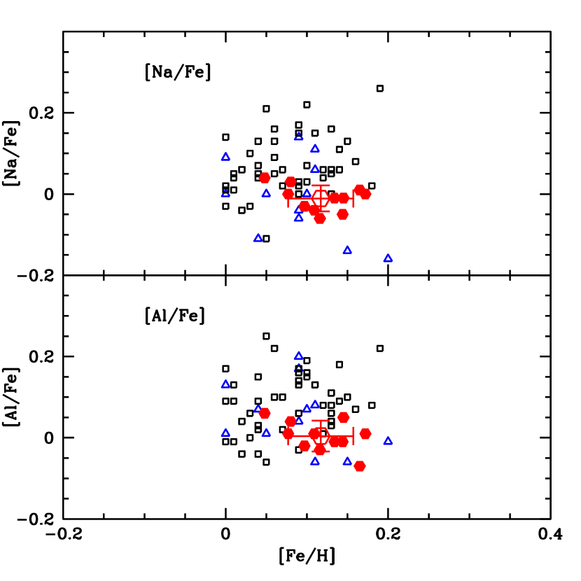
We also found abundances for some other elements of interest. We have measured equivalent widths of two lines of Na I, one Al I line, two lines of Sc II, and two lines of V I. (Reddy et al. (2003) showed in test calculations that the effects of hyperfine splitting on the lines they used of V I and Sc II have virtually no effect on the abundances derived; we used those same lines.) Figure 14 shows the results for Na and Al. The value for [Na/Fe] and [Al/Fe] are solar at 0.011 0.032 and 0.004 0.038, respectively, and are in good agreement with the field star sample. See 5 for an interesting comparison with Na in the Praesepe giants.
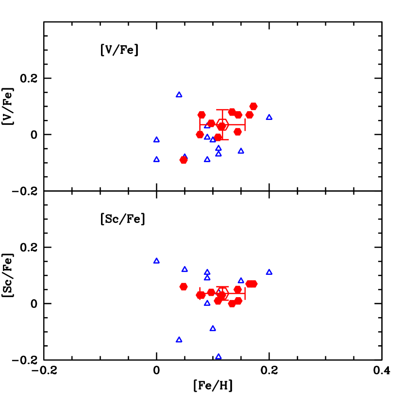
In Figure 15 we show the results for V and Sc. The ratios of [V/Fe] and [Sc/Fe] are somewhat greater than solar at +0.035 0.053 and 0.036 0.024, respectively, but they are basically solar within the errors. The field stars from the Reddy papers are similar, but, as expected, they have greater scatter compared to the cluster stars.
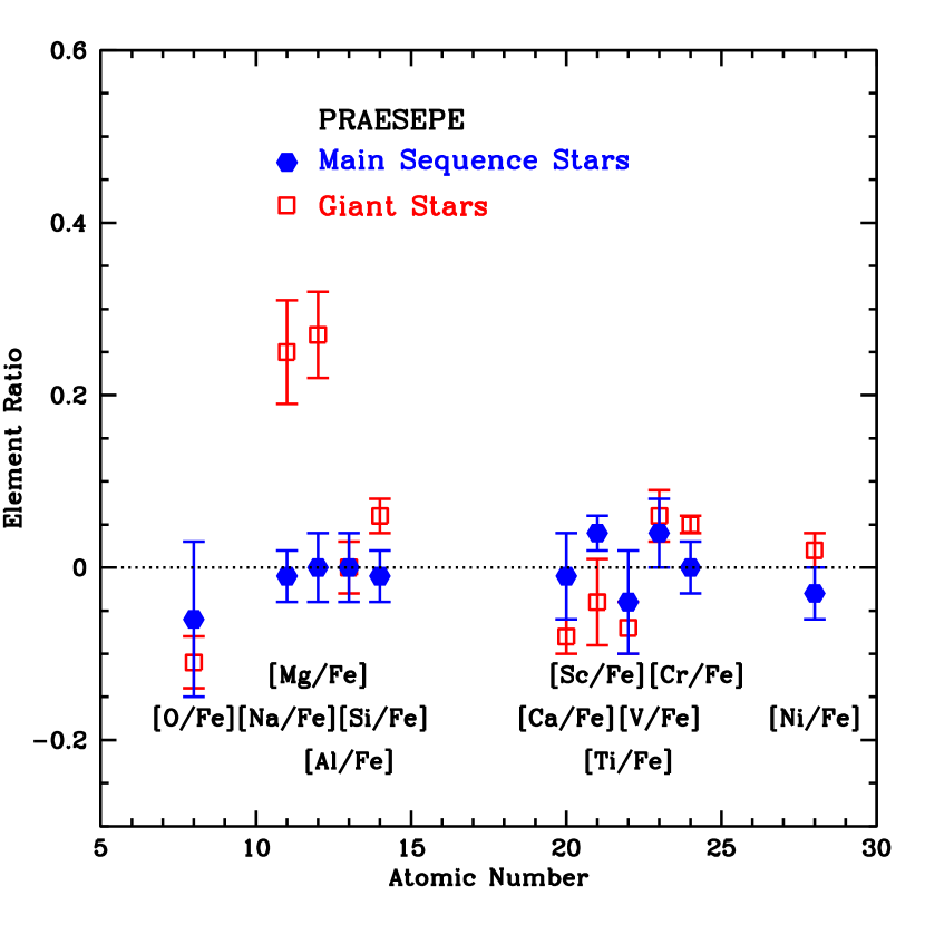
5 COMPARISON WITH PRAESEPE GIANTS
Carrera & Pancino (2011) determined abundances of many elements in three red giants in Praesepe. We can compare our results for solar-temperature dwarf stars with theirs for the red giants. Table 9 and Figure 17 show those comparisons. Our values for [Fe/H] are in good agreement within our 1 sigma errors.
Their results for [Na/Fe] show an enhancement to +0.25 0.06 from our solar value ([Na/Fe] = 0.01 0.03). Our two studies have used the same Na lines and the same gf values. The lines selected are weak Na lines and expected to have only minor NLTE corrections, e.g. Asplund (2005). Each of their three red giants shows the enhancement of [Na/Fe]: +0.23, +0.30, +0.18. Such a Na-enhancement could be the result of proton-capture nucleosynthesis in the Ne Na cycling with dredge-up into the atmospheres of the red giants. Enhanced Na and an anti-correlation between Na and O has been discovered recently in evolved red giants in the populous old open cluster, NGC 6791, by Geisler et al. (2012). There are too few stars in Praesepe that have evolved to become red giants to detect any such effect in Praesepe. All three giants studied by Carrera & Pancino (2011) do have low [O/Fe] at 0.11 0.03.
For the alpha elements, Si, Ca, and Ti, the agreement is very good and close to solar in both dwarfs and giants. However, Carrera & Pancino (2011) found [Mg/Fe] is enhanced to +0.27 in the giants. Our value for the dwarf stars is solar. Their three giants give similar values for [Mg/Fe]: +0.22, +0.27, +0.31. Our two studies have measured different lines of Mg I. Two of their four lines are quite strong at more than 100 mÅ. It is not expected that Mg would be increased in the giants, rather the Mg Al cycling would result in a decrease in Mg. Yong et al. (2003) find a positive correlation between Al and Mg for some giant stars in the globular cluster, NGC 6752, apparently due to an increase in 26Mg (see their Figure 12). It might be interesting to determine the Mg isotope ratios in those giant stars. On the other hand, the [Al/Fe] abundances in both the dwarfs and the giants in Praesepe are solar.
Our Ba abundances are from the Ba II line at 5853 Å in which we included the hyperfine structure of that line. Our mean cluster abundance for [Ba/Fe] is +0.11 0.04 for the main sequence stars which is consistent with the findings of D’Orazi et al. (2009) discussed in 4.6. Carrera & Pancino (2011) found [Ba/Fe] is +0.33 0.05 for their three giants. This could be evidence for n-capture-enriched Ba in the giants. However, apparently Carrera & Pancino (2011) did not use the hyperfine splitting (hfs) in their Ba analysis. In order to determine the effect of the hfs on the Ba abundance, we determined Ba abundances without including the hfs for our 11 dwarf stars. We find that including the hfs reduces the Ba abundance by 0.03 dex. If the correction is similar for giants, then [Ba/Fe] would be +0.30 in those three giants; this is still an increase over [Ba/Fe] in the dwarfs.
6 SUMMARY AND CONCLUSIONS
We have analyzed high-resolution, high S/N spectra of 11 solar-temperature main sequence stars in the Praesepe open cluster obtained with Keck I + HIRES. The spectra cover a region from 5730 – 8140 Å. We have determined stellar temperatures from the infrared flux method and found Fe abundances from some 55 Fe I lines and 6 Fe II lines in each star. The [Fe/H] agreement between the Fe I and Fe II lines is excellent and the cluster mean is [Fe/H] = 0.12 0.04 (0.01).
We determined Li abundances by the spectral synthesis method and found them to track the Hyades Li abundances very well showing a steady decline from 6000 K to 5650 K; the decline is due to increasing Li depletion at decreasing temperatures. We find that [C/Fe] and [O/Fe] to be 0.14 0.07 and 0.15 0.09, respectively. These values are similar, but somewhat lower than the field star samples and we interpret the lower values to be due to the younger age of Praesepe relative to the field stars. This follows the steady decline in [C/Fe] and [O/Fe] over time from the early excess of C and O over Fe as produced by the most massive stars and SN II followed by the rise in Fe from SN Ia. All the -elements, [Mg/Fe], [Si/Fe], [Ca/Fe], and [Ti/Fe] are solar at 0.00 0.04, 0.01 0.03, 0.01 0.05, and 0.04 0.06, respectively. As is the case for [C/Fe] and [O/Fe], the -elements, Mg, Ti, and Si, are somewhat lower relative to Fe compared to the field stars. For [Ca/Fe] the field star sample is also solar and has less spread in the values.
The abundances of the Fe-peak elements, [Cr/Fe] and [Ni/Fe], were found to track Fe and are basically solar at 0.00 0.03 and 0.03 0.03, respectively. The n-capture element Y from the first s-process peak was found to be solar at [Y/Fe] = 0.01 0.08 and in good agreement with the field stars. The n-capture element Ba from the second s-process peak was found to be enhanced relative to solar and relative to the field stars with [Ba/Fe] = +0.11 0.04. For the Praesepe stars [V/Fe], [Sc/Fe], [Na/Fe], and [Al/Fe] are essentially solar at 0.04 0.05, 0.04 0.02, 0.01 0.03, and 0.00 0.04, respectively. Both [Na/Fe] and [Al/Fe] are somewhat lower than the field stars and have less spread in the values, as expected in a cluster of stars of common origin.
The comparison with the composition of the giant stars in Praesepe yielded some interesting differences for Na, Mg, and Ba. The three red giants studied by Carrera & Pancino (2011) show an enhancement in [Na/Fe] of +0.26 compared to our dwarf stars. The enhancement of Na might be caused by the proton-capture nucleosynthesis in the Ne Na cycling in the interior and subsequent dredge-up in the giant stars. For the -elements Si, Ca, and Ti the dwarfs and the giants are similar within the errors. However, they found an enhancement in [Mg/Fe] in the giants of +0.27. If there is Mg Al cycling, that would lead to a decrease in [Mg/Fe] and an increase in [Al/Fe]; for both dwarfs and giants [Al/Fe] = 0.00 with similar uncertainties 0.04. It may be important to measure the Mg isotopes in the giants in case the increase in Mg is due to an increase in 26Mg. Barium appears to be enhanced in the giants as well. We find [Ba/Fe] = +0.11 0.04 for the dwarf stars while they derive +0.33 0.05. The giants may be enriched by the s-process n-capture. However, there is no apparent enrichment of [Y/Fe] in the giants.
References
- (1)
- (2)
- (3) An, D., Terndrup, D.M., Pinsonneault, M.H., Paulson, D., Hanson, R.B. & Stauffer, J. 2007, ApJ, 655, 233-260
- (4) Asplund, M. 2005, ARAA, 43, 481
- (5) Balachandran, S. 1995, ApJ, 446, 203
- (6) Barrado y Navascues, D., Stauffer, J. & Randich, S. 1998, ApJ, 506, 347-359
- (7) Bergemann, M. & Cescutti, G. 2010, A&A, 522, A9
- (8) Boesgaard, A.M. 1989, ApJ, 336, 798
- (9) Boesgaard, A.M. & Budge, K.G. 1988, ApJ, 332, 410
- (10) Boesgaard, A. M., King, J. R., Deliyannis, C. P. & Vogt, S. S. 1999, AJ, 117, 492
- (11) Carrera, R. & Pancino, E. 2011, A&A, 535, A30
- (12) Casagrande, L., Ram rez, I., Mel ndez, J., Bessell, M. & Asplund, M. 2010 A&A, 512, 54
- (13) Clayton, D. 2003 “Handbook of Isotopes in the Cosmos,”
- (14) D’Orazi, V., Magrini, L., Randich, S., Galli, D., Busso, M. & Sestito, P. 2009, ApJ, 693, L31.
- (15) Edvardsson, B., Andersen, J., Gustafsson, B., Lambert, D.L., Nissen, P.E. & Tomkin, J. 1993, A&A, 275, 101-150
- (16) Eggen, O.J. 1992, AJ, 104, 1482
- (17) Franciosini, E., Randich, S. & Pallavicini, R. 2003, A&A, 405, 551-561
- (18) Friel, E.D. & Boesgaard, A.M. 1992, ApJ, 387, 170
- (19) Geisler, D., Villanova, S., Carraro, G., Pilachowski, C., Cummings, J., Johnson, C. I. & Bresolin, F. 2012 A&A, 756, 40
- (20) Gratton, R. 2000, in “Stellar Clusters and Associations” eds. R. Pallavicini, G. Micela & S. Sciortino (San Francisco: A.S.P) ASPC, 198, 225
- (21) Gray, D.F. 1976 in “The Observation and Analysis of Stellar Photospheres” (New York: John Wiley & Sons) p. 389
- (22) Hannaford, P, Lowe, R.M., Grevesse, N., Biemont, E. & Whaling, W. 1982, ApJ, 261, 736
- (23) Holland, K., Jameson, R.F., Hodgkin, S., Davies, M.B. & Pinfield, D. 2000, MNRAS, 319, 956
- (24) Israelian, G., Garc a L pez, R.J. & Rebolo, R. 1998, ApJ, 507, 885
- (25) Israelian, G., Rebolo, R., Garc a L pez, R.J., Bonifacio, P., Molaro, P. Basri, G. & Shchukina, N. 2001, ApJ, 551, 833
- (26) Johnson, H.L. 1952, ApJ, 116, 640
- (27) Jones, B.F. & Cudworth, K.M. 1983, AJ, 88, 215
- (28) Jones, B.F. & Stauffer, J.R. 1991, AJ102, 1080
- (29) King, J.R. & Hiltgen, D. 1996, PASP, 108, 246
- (30) Kraft, R.P., Sneden, C., Smith, G.H., Shetrone, M.D., Langer, G. E. & Pilachowski, C.A. 1997 AJ, 113, 279
- (31) Kurucz, R. L. 1993, CD-ROM 13 (Cambridge: Smithsonian Astrophys. Obs.)
- (32) Kurucz, R.L. 1995, CD-ROM No. 23. Cambridge, Mass.: Smithsonian Astrophysical Observatory
- (33) Magrini, L., Sestito, P., Randich, S. & Galli, D. 2009, A&A, 494, 95-108
- (34) Mendoza, E.E. 1967, Bol. Obs. Tonantzintla Tacubaya, 4, 149
- (35) Mermilliod, J.C. & Mayor, M. 1999, A&A, 352, 479
- (36) Pace, G., Pasquini, L. & Francois, P. 2008, A&A, 489, 403-412
- (37) Palous, J., Ruprecht, J., Dluzhnevskaya, O.B. & Piskunov, T. 1977, A&A, 61, 27-37
- (38) Randich, S. & Schmitt, J.H.M.M. 1995, A&A, 298, 115-132
- (39) Reddy, B., Lambert, D.L. & Allende Prieto, C. 2006, MNRAS, 367, 1329
- (40) Reddy, B., Tompkin, J., Lambert, D.L. & Allende Prieto, C. 2003, MNRAS, 340, 304
- (41) Rentzsch-Holm, I. 1996, A&A, 312, 966
- (42) Salaris, M., Weiss, A. & Percival, S.M. 2004, A&A, 414, 163-174
- (43) Sneden, C. 1973, PhD thesis, Univ. of Texas, Austin
- (44) Sneden, C., Kraft, R.P., Prosser, C.F. & Langer, G. E. 1991, AJ, 102, 2001
- (45) Sobeck, J.S., Lawler, J.E. & Sneden, C. 2007, ApJ, 667, 1267
- (46) Soderblom, D.R., Fedele, S.B., Jones, B.F., Stauffer, J. R. & Prosser, C.F. 1993, AJ, 106, 1080
- (47) Soderblom, D.R., Fedele, S.B., Jones, B.F., Stauffer, J. R. & Prosser, C.F. 1995, AJ, 109, 1402
- (48) Stern, R.A., Schmitt, J.H.M.M. & Kahabka, P.T. 1995, ApJ, 448, 683-704
- (49) Stephens, A. 1999, AJ, 117, 1771
- (50) Stephens, A. & Boesgaard, A.M. 2002, AJ, 123, 1647
- (51) Takeda, Y. 2003, A&A, 402, 343
- (52) Takeda, Y. & Honda, S. 2005, PASJ, 57, 65
- (53) Tinsley, B.M. 1980, Fund. Cosmic Phys. 5, 287
- (54) Tsujimoto, T., Yoshii, Y., Nomoto, K. & Shigeyama, T. 1995, A&A, 302, 704
- (55) Vogt, S. S., Allen, S. L., Bigelow, B. C., Bresee, L., Brown, B., Cantrall, T., Conrad, A., Couture, M., Delaney, C., Epps, H. W., and 17 coauthors 1994, SPIE, 2198, 362
- (56) Weise, W.L., Fuhr, J.R., & Deters, T.M. (1996), in Atomic Transition Probabilities of Carbon, Nitrogen, and Oxygen: A Critical Data Compilation. NIST, QC 453 Wheeler, J. C., Sneden, C. & Truran, J.W., Jr. 1989, ARA&A, 27, 279
- (57) Yong, D., Grundahl, F., Lambert, D.L., Nissen, P.E. & Shetrone, M.D. 2003, A&A, 402, 985
- (58)
| Star | V | B-V | ref.11 1 = Mendoza (1967), 2 = Johnson (1952) | Night | Exp. Time | Total |
|---|---|---|---|---|---|---|
| UT | (min) | S/N | ||||
| KW 23 | 11.29 | 0.710 | 1 | 11 Jan 2003 | 25 | 149 |
| KW 30 | 11.40 | 0.730 | 1 | 11 Jan 2003 | 25 | 141 |
| KW 58 | 11.26 | 0.671 | 2 | 11 Feb 2003 | 25 | 159 |
| KW 181 | 10.47 | 0.588 | 2 | 11 Jan 2003 | 10 | 93 |
| KW 208 | 10.66 | 0.583 | 2 | 11 Jan 2003 | 14 | 153 |
| KW 288 | 10.69 | 0.593 | 2 | 11 Feb 2003 | 15 | 150 |
| KW 301 | 11.17 | 0.655 | 2 | 11 Feb 2003 | 25 | 155 |
| KW 335 | 11.03 | 0.651 | 2 | 11 Jan 2003 | 20 | 156 |
| KW 399 | 11.93 | 0.624 | 2 | 11 Jan 2003 | 20 | 166 |
| KW 432 | 11.05 | 0.646 | 2 | 11 Feb 2003 | 20 | 143 |
| KW 508 | 10.77 | 0.594 | 2 | 11 Jan 2003 | 20 | 159 |
| Star | B | V | J | H | K | Vc | V-Rc | RcIc | VIc |
|---|---|---|---|---|---|---|---|---|---|
| KW 23 | 12.00 | 11.29 | 10.075 | 9.780 | 9.686 | ||||
| KW 30 | 12.13 | 11.40 | 10.187 | 9.898 | 9.803 | ||||
| KW 58 | 11.93 | 11.26 | 10.079 | 9.791 | 9.689 | ||||
| KW 181 | 11.06 | 10.47 | 9.357 | 9.088 | 8.997 | 10.488 | 0.339 | 0.325 | 0.664 |
| KW 208 | 11.24 | 10.66 | 9.565 | 9.357 | 9.259 | ||||
| KW 288 | 11.28 | 10.69 | 9.640 | 9.401 | 9.336 | 10.698 | 0.333 | 0.308 | 0.641 |
| KW 301 | 11.83 | 11.17 | 10.012 | 9.698 | 9.655 | ||||
| KW 335 | 11.68 | 11.03 | 9.864 | 9.588 | 9.507 | ||||
| KW 399 | 11.55 | 10.93 | 9.812 | 9.549 | 9.469 | ||||
| KW 432 | 11.70 | 11.05 | 9.869 | 9.627 | 9.544 | ||||
| KW 508 | 11.36 | 10.77 | 9.659 | 9.416 | 9.359 | 10.761 | 0.334 | 0.326 | 0.660 |
| Star | TB-V | TV-J | TV-H | TV-Ic | TV-Rc | TRc-Ic | mean Teff | |
|---|---|---|---|---|---|---|---|---|
| KW 23 | 5615 | 5703 | 5772 | 5697 | 79 | |||
| KW 30 | 5554 | 5708 | 5770 | 5677 | 111 | |||
| KW 58 | 5697 | 5771 | 5813 | 5761 | 59 | |||
| KW 181 | 5922 | 5910 | 5954 | 5868 | 5918 | 5824 | 5899 | 46 |
| KW 208 | 5978 | 5950 | 6065 | 5997 | 60 | |||
| KW 288 | 6006 | 6050 | 6078 | 5958 | 5954 | 5988 | 6006 | 50 |
| KW 301 | 5776 | 5815 | 5836 | 5809 | 30 | |||
| KW 335 | 5861 | 5800 | 5867 | 5842 | 37 | |||
| KW 399 | 5874 | 5901 | 5932 | 5903 | 29 | |||
| KW 432 | 5841 | 5768 | 5914 | 5841 | 73 | |||
| KW 508 | 5958 | 5919 | 5951 | 5887 | 5943 | 5831 | 5915 | 48 |
| Star | [FeI/H] | num. | [FeII/H] | num. | mean [Fe/H] | ||
|---|---|---|---|---|---|---|---|
| KW 23 | 0.15 | 0.08 | 54 | 0.09 | 0.11 | 6 | 0.144 |
| KW 30 | 0.12 | 0.08 | 55 | 0.08 | 0.09 | 6 | 0.116 |
| KW 58 | 0.11 | 0.09 | 55 | 0.10 | 0.06 | 6 | 0.109 |
| KW 181 | 0.13 | 0.10 | 50 | 0.29 | 0.09 | 5 | 0.145 |
| KW 208 | 0.10 | 0.10 | 55 | 0.07 | 0.09 | 6 | 0.097 |
| KW 288 | 0.08 | 0.09 | 54 | 0.08 | 0.07 | 6 | 0.080 |
| KW 301 | 0.17 | 0.09 | 55 | 0.12 | 0.09 | 6 | 0.165 |
| KW 335 | 0.14 | 0.09 | 55 | 0.08 | 0.09 | 6 | 0.134 |
| KW 399 | 0.08 | 0.09 | 55 | 0.05 | 0.09 | 6 | 0.077 |
| KW 432 | 0.18 | 0.09 | 55 | 0.10 | 0.09 | 6 | 0.172 |
| KW 508 | 0.04 | 0.10 | 55 | 0.13 | 0.06 | 6 | 0.048 |
| Star | log g | [Fe/H] | ||
|---|---|---|---|---|
| KW 23 | 5699 | 4.43 | 0.12 | 1.10 |
| KW 30 | 5675 | 4.44 | 0.12 | 1.07 |
| KW 58 | 5761 | 4.42 | 0.12 | 1.16 |
| KW 181 | 5899 | 4.39 | 0.12 | 1.31 |
| KW 208 | 5997 | 4.38 | 0.12 | 1.40 |
| KW 288 | 6006 | 4.38 | 0.12 | 1.41 |
| KW 301 | 5809 | 4.41 | 0.12 | 1.21 |
| KW 335 | 5842 | 4.40 | 0.12 | 1.26 |
| KW 399 | 5903 | 4.40 | 0.12 | 1.31 |
| KW 432 | 5841 | 4.40 | 0.12 | 1.25 |
| KW 508 | 5915 | 4.39 | 0.12 | 1.33 |
| KW 23 | KW 30 | KW 58 | KW 181 | KW 208 | KW 288 | KW 301 | KW 335 | KW 399 | KW 432 | KW 508 | mean | ||
|---|---|---|---|---|---|---|---|---|---|---|---|---|---|
| Fe/H | 0.144 | 0.116 | 0.109 | 0.145 | 0.097 | 0.080 | 0.163 | 0.134 | 0.077 | 0.172 | 0.048 | 0.117 | 0.039 |
| A(Li) | 1.88 | 2.02 | 2.22 | 2.47 | 2.80 | 2.75 | 2.42 | 2.54 | 2.64 | 2.45 | 2.68 | ||
| C/Fe | 0.14 | 0.04 | 0.04 | 0.01 | 0.12 | 0.14 | 0.12 | 0.12 | 0.11 | 0.12 | 0.03 | 0.090 | 0.048 |
| O/Fen | 0.19 | 0.10 | 0.19 | 0.01 | 0.18 | 0.13 | 0.18 | 0.14 | 0.23 | 0.28 | 0.02 | 0.146 | 0.089 |
| Na/Fe | 0.05 | 0.06 | 0.04 | 0.01 | 0.03 | 0.03 | 0.01 | 0.01 | 0.00 | 0.00 | 0.04 | 0.011 | 0.032 |
| Mg/Fe | 0.04 | 0.02 | 0.02 | 0.07 | 0.03 | 0.04 | 0.01 | 0.02 | 0.02 | 0.01 | 0.07 | 0.003 | 0.040 |
| Al/Fe | 0.01 | 0.03 | 0.01 | 0.05 | 0.02 | 0.04 | 0.07 | 0.01 | 0.01 | 0.01 | 0.06 | 0.004 | 0.038 |
| Si/Fe | 0.04 | 0.02 | 0.01 | 0.04 | 0.03 | 0.02 | 0.02 | 0.01 | 0.01 | 0.04 | 0.05 | 0.005 | 0.031 |
| Ca/Fe | 0.06 | 0.00 | 0.01 | 0.01 | 0.06 | 0.02 | 0.00 | 0.04 | 0.01 | 0.06 | 0.04 | 0.006 | 0.049 |
| Sc/Fe | 0.05 | 0.03 | 0.01 | 0.01 | 0.04 | 0.03 | 0.07 | 0.00 | 0.03 | 0.07 | 0.06 | 0.036 | 0.024 |
| Ti/Fe | 0.03 | 0.02 | 0.02 | 0.06 | 0.11 | 0.08 | 0.06 | 0.04 | 0.07 | 0.10 | 0.05 | 0.033 | 0.059 |
| V/Fe | 0.01 | 0.03 | 0.02 | 0.04 | 0.06 | 0.11 | 0.02 | 0.07 | 0.04 | 0.05 | 0.02 | 0.037 | 0.036 |
| Cr/Fe | 0.01 | 0.01 | 0.02 | 0.06 | 0.02 | 0.00 | 0.03 | 0.00 | 0.01 | 0.04 | 0.05 | 0.003 | 0.031 |
| Ni/Fe | 0.01 | 0.05 | 0.01 | 0.07 | 0.03 | 0.03 | 0.01 | 0.02 | 0.05 | 0.01 | 0.06 | 0.028 | 0.027 |
| Y/Fe | 0.15 | 0.08 | 0.06 | 0.07 | 0.11 | 0.08 | 0.05 | 0.01 | 0.01 | 0.00 | 0.01 | 0.007 | 0.077 |
| Ba/Fe | 0.13 | 0.13 | 0.10 | 0.10 | 0.08 | 0.05 | 0.18 | 0.14 | 0.08 | 0.13 | 0.11 | 0.112 | 0.035 |
| Star | Teff | log g | [Fe/H] | Total | |
|---|---|---|---|---|---|
| 75 K | 0.20 | 0.10 | 0.20 | ||
| KW 23 | 0.05 | 0.01 | 0.01 | 0.03 | 0.060 |
| KW 30 | 0.04 | 0.02 | 0.00 | 0.04 | 0.060 |
| KW 58 | 0.05 | 0.01 | 0.01 | 0.04 | 0.060 |
| KW 181 | 0.05 | 0.01 | 0.00 | 0.01 | 0.059 |
| KW 208 | 0.05 | 0.01 | 0.00 | 0.03 | 0.059 |
| KW 288 | 0.04 | 0.01 | 0.00 | 0.05 | 0.059 |
| KW 301 | 0.05 | 0.01 | 0.00 | 0.04 | 0.065 |
| KW 335 | 0.05 | 0.01 | 0.00 | 0.03 | 0.059 |
| KW 399 | 0.05 | 0.01 | 0.01 | 0.03 | 0.060 |
| KW 432 | 0.05 | 0.01 | 0.00 | 0.04 | 0.065 |
| KW 508 | 0.05 | 0.01 | 0.00 | 0.01 | 0.060 |
| Star | Element | Teff | log g | [Fe/H] | Total | |
|---|---|---|---|---|---|---|
| 75 K | 0.20 | 0.10 | 0.20 | |||
| KW 23 | C I | 0.06 | 0.07 | 0.01 | 0.00 | 0.093 |
| O I | 0.08 | 0.05 | 0.00 | 0.01 | 0.095 | |
| Na I | 0.07 | 0.00 | 0.03 | 0.02 | 0.079 | |
| Mg I | 0.03 | 0.02 | 0.00 | 0.01 | 0.037 | |
| Al I | 0.04 | 0.01 | 0.00 | 0.01 | 0.042 | |
| Si I | 0.01 | 0.00 | 0.02 | 0.01 | 0.024 | |
| Ca I | 0.06 | 0.04 | 0.01 | 0.04 | 0.083 | |
| Sc II | 0.00 | 0.09 | 0.03 | 0.02 | 0.097 | |
| Ti I | 0.07 | 0.01 | 0.00 | 0.01 | 0.071 | |
| V I | 0.09 | 0.00 | 0.00 | 0.01 | 0.091 | |
| Cr I | 0.06 | 0.01 | 0.01 | 0.02 | 0.065 | |
| Ni I | 0.04 | 0.01 | 0.01 | 0.05 | 0.066 | |
| Y I | 0.11 | 0.01 | 0.00 | 0.00 | 0.110 | |
| Y II | 0.01 | 0.09 | 0.02 | 0.02 | 0.095 | |
| Ba II | 0.03 | 0.05 | 0.11 | 0.11 | 0.166 | |
| KW 208 | C I | 0.04 | 0.05 | 0.01 | 0.01 | 0.066 |
| O I | 0.05 | 0.03 | 0.00 | 0.02 | 0.062 | |
| Na I | 0.06 | 0.00 | 0.02 | 0.01 | 0.064 | |
| Mg I | 0.03 | 0.01 | 0.01 | 0.00 | 0.037 | |
| Al I | 0.04 | 0.00 | 0.00 | 0.00 | 0.040 | |
| Si I | 0.02 | 0.01 | 0.01 | 0.01 | 0.026 | |
| Ca I | 0.06 | 0.04 | 0.00 | 0.04 | 0.082 | |
| Sc II | 0.01 | 0.07 | 0.03 | 0.02 | 0.079 | |
| Ti I | 0.07 | 0.00 | 0.00 | 0.01 | 0.071 | |
| V I | 0.08 | 0.00 | 0.00 | 0.01 | 0.081 | |
| Cr I | 0.04 | 0.02 | 0.01 | 0.02 | 0.050 | |
| Ni I | 0.05 | 0.01 | 0.00 | 0.04 | 0.065 | |
| Y I | 0.10 | 0.00 | 0.00 | 0.00 | 0.100 | |
| Y II | 0.00 | 0.08 | 0.03 | 0.01 | 0.086 | |
| Ba II | 0.03 | 0.06 | 0.04 | 0.09 | 0.119 | |
| KW 335 | C I | 0.06 | 0.06 | 0.01 | 0.01 | 0.086 |
| O I | 0.06 | 0.04 | 0.01 | 0.01 | 0.074 | |
| Na I | 0.07 | 0.01 | 0.02 | 0.03 | 0.079 | |
| Mg I | 0.03 | 0.02 | 0.00 | 0.00 | 0.036 | |
| Al I | 0.03 | 0.01 | 0.00 | 0.01 | 0.033 | |
| Si I | 0.02 | 0.01 | 0.02 | 0.01 | 0.032 | |
| Ca I | 0.05 | 0.04 | 0.00 | 0.04 | 0.076 | |
| Sc II | 0.00 | 0.09 | 0.04 | 0.02 | 0.100 | |
| Ti I | 0.07 | 0.00 | 0.00 | 0.01 | 0.071 | |
| V I | 0.07 | 0.01 | 0.00 | 0.02 | 0.074 | |
| Cr I | 0.06 | 0.01 | 0.00 | 0.02 | 0.064 | |
| Ni I | 0.05 | 0.01 | 0.01 | 0.04 | 0.066 | |
| Y I | 0.10 | 0.00 | 0.00 | 0.00 | 0.100 | |
| Y II | 0.00 | 0.09 | 0.03 | 0.01 | 0.095 | |
| Ba II | 0.02 | 0.05 | 0.03 | 0.11 | 0.126 |
| element | Dwarfs | Giants | ||
|---|---|---|---|---|
| Fe/H | +0.12 | 0.04 | +0.16 | 0.05 |
| O/Fe | 0.06 | 0.09 | 0.11 | 0.03 |
| Na/Fe | 0.01 | 0.03 | +0.25 | 0.06 |
| Mg/Fe | 0.00 | 0.04 | +0.27 | 0.05 |
| Al/Fe | 0.00 | 0.04 | 0.00 | 0.03 |
| Si/Fe | 0.01 | 0.03 | +0.06 | 0.02 |
| Ca/Fe | 0.01 | 0.05 | 0.08 | 0.02 |
| Sc/Fe | +0.04 | 0.02 | 0.04 | 0.05 |
| Ti/Fe | 0.04 | 0.06 | 0.07 | 0.03 |
| V/Fe | +0.04 | 0.04 | +0.06 | 0.03 |
| Cr/Fe | +0.00 | 0.03 | +0.05 | 0.01 |
| Ni/Fe | 0.03 | 0.03 | +0.02 | 0.02 |
| Y/Fe | +0.01 | 0.08 | 0.11 | 0.01 |
| Ba/Fe | +0.11 | 0.04 | +0.33 | 0.05 |


| Ion | (Å) | Ex. Pot. (eV) | KW 23 | KW 208 | KW 335 | |
|---|---|---|---|---|---|---|
| C I | 6587.62 | 8.53 | 1.000 | 13.1 | 19.6 | |
| 7100.13 | 8.64 | 1.020 | 11.8 | 17.8 | ||
| 7111.45 | 8.64 | 1.080 | 10.8 | 16.6 | 13.5 | |
| 7113.17 | 8.65 | 0.770 | 24.0 | 29.1 | 28.6 | |
| 7115.17 | 8.64 | 0.930 | 25.3 | 32.6 | ||
| 7116.96 | 8.65 | 0.900 | 18.0 | 27.5 | 19.9 | |
| 7119.70 | 8.64 | 1.220 | 11.3 | |||
| O I | 6158.17 | 10.74 | 0.320 | 5.7 | ||
| 7771.94 | 9.11 | +0.369 | 72.8 | 107.2 | 90.5 | |
| 7774.17 | 9.11 | +0.223 | 60.2 | 91.7 | 75.1 | |
| 7775.39 | 9.11 | +0.002 | 53.3 | 78.5 | 61.6 | |
| Na I | 6154.227 | 2.10 | 1.660 | 46.6 | 35.5 | 41.6 |
| 6160.751 | 2.10 | 1.350 | 65.8 | 51.8 | 64.4 | |
| Mg I | 6965.41 | 5.75 | 1.870 | 27.6 | 21.0 | 26.5 |
| 7387.70 | 5.75 | .200 | 87.4 | 74.8 | 90.2 | |
| Al I | 6698.67 | 3.14 | 1.950 | 25.7 | 18.2 | 22.4 |
| Si I | 5772.15 | 5.08 | 1.750 | 61.2 | 57.3 | 61.2 |
| 5948.55 | 5.08 | 1.225 | 98.2 | 94.1 | 97.2 | |
| 6125.03 | 5.61 | 1.540 | 39.3 | 37.7 | 39.4 | |
| 6142.49 | 5.62 | 1.480 | 40.0 | 41.0 | 42.0 | |
| 6155.14 | 5.62 | 0.840 | 98.4 | 97.1 | 96.2 | |
| 6848.57 | 5.86 | 1.740 | 20.4 | 19.1 | 20.6 | |
| 7003.57 | 5.96 | 0.860 | 68.6 | 71.5 | 70.5 | |
| 7005.90 | 5.98 | 0.680 | 91.4 | 94.6 | 93.8 | |
| 7289.19 | 5.62 | 0.620 | ||||
| 7405.79 | 5.61 | 0.570 | 102.1 | 100.4 | 100.6 | |
| 7760.64 | 6.20 | 1.280 | 18.3 | 24.9 | 32.6 | |
| Ca I | 6161.30 | 2.52 | 1.270 | 84.8 | 58.9 | 77.8 |
| 6163.76 | 2.52 | 1.286 | 81.2 | 85.3 | ||
| 6166.44 | 2.52 | 1.140 | 81.9 | 68.7 | 74.6 | |
| 6169.04 | 2.52 | 0.797 | 97.4 | 107.0 | ||
| 6169.56 | 2.53 | 0.374 | 115.1 | |||
| 6449.81 | 2.52 | 0.502 | 109.9 | |||
| 6455.60 | 2.52 | 1.340 | 69.0 | 51.9 | 67.1 | |
| 6464.68 | 2.52 | 2.530 | 22.1 | 9.4 | 15.5 | |
| 6471.66 | 2.53 | 0.638 | 96.5 | 102.6 | ||
| 6499.65 | 2.52 | 0.818 | 103.2 | 89.6 | 96.2 | |
| Sc II | 6245.61 | 1.51 | 1.150 | 37.6 | 38.6 | 36.9 |
| 6604.60 | 1.36 | 1.230 | 39.7 | 40.2 | 38.1 | |
| Ti I | 5866.46 | 1.07 | 0.870 | 57.7 | 38.6 | 51.0 |
| 6126.22 | 1.07 | 1.460 | 30.5 | 15.5 | 22.6 | |
| 6554.24 | 1.44 | 1.160 | 23.2 | 7.8 | 13.6 | |
| 6556.08 | 1.46 | 1.100 | 26.3 | 13.9 | 19.6 | |
| 6599.11 | 0.90 | 2.060 | 13.5 | 9.6 | ||
| 6745.55 | 2.24 | 1.100 | 4.2 | |||
| 7138.93 | 1.44 | 1.720 | 11.0 | 7.1 | ||
| 7216.19 | 1.44 | 1.300 | 26.3 | 10.8 | 15.9 | |
| 7251.72 | 1.43 | 0.860 | 54.7 | 35.4 | 47.7 | |
| 7440.58 | 2.25 | 1.080 | 7.6 | 9.0 | ||
| 7949.15 | 1.50 | 1.430 | 15.8 | 10.5 | ||
| V I | 6216.31 | 0.28 | 0.830 | 48.1 | 33.8 | 45.3 |
| 6504.14 | 1.18 | 0.740 | 18.2 | 11.1 | 15.9 | |
| Cr I | 5783.09 | 3.32 | -0.500 | 45.4 | 33.1 | 38.0 |
| 5783.89 | 3.32 | 0.295 | 60.8 | 43.7 | 53.8 | |
| 6330.09 | 0.94 | 2.920 | 39.5 | 34.5 | ||
| 6501.20 | 0.98 | 3.660 | 12.6 | 12.0 | ||
| 6605.57 | 4.14 | 0.810 | ||||
| 6630.03 | 1.03 | 3.560 | 12.3 | 9.3 | 10.7 | |
| 6978.48 | 3.46 | +0.143 | 81.1 | 65.7 | 70.9 | |
| 6979.81 | 3.46 | 0.460 | 49.2 | 38.5 | 43.3 | |
| 6980.91 | 3.46 | 1.120 | 16.4 | 10.3 | 9.6 | |
| Fe I | 5775.08 | 4.22 | 1.300 | 70.5 | 59.5 | 65.4 |
| 5809.22 | 3.88 | 1.760 | 64.5 | 51.6 | 59.0 | |
| 5849.69 | 3.69 | 2.970 | 11.2 | 5.1 | 8.8 | |
| 5852.22 | 4.55 | 1.220 | 51.9 | 41.4 | 47.7 | |
| 5855.08 | 4.61 | 1.560 | 28.5 | 22.3 | 25.5 | |
| 5856.09 | 4.29 | 1.600 | 42.5 | 33.4 | 39.1 | |
| 5858.78 | 4.22 | 2.190 | 17.6 | 14.3 | 17.6 | |
| 5859.59 | 4.55 | 0.610 | 83.3 | 76.2 | 82.8 | |
| 5861.11 | 4.28 | 2.340 | 10.4 | 7.8 | 8.9 | |
| 5862.36 | 4.55 | 0.420 | 101.8 | 93.3 | 102.1 | |
| 6027.05 | 4.08 | 1.150 | 73.8 | 66.6 | 72.8 | |
| 6055.99 | 4.73 | 0.460 | 84.8 | 78.9 | 82.2 | |
| 6127.90 | 4.14 | 1.399 | 58.7 | 50.7 | 55.2 | |
| 6151.62 | 2.18 | 3.299 | 59.8 | 44.1 | 55.8 | |
| 6157.73 | 4.07 | 1.270 | 71.9 | 65.0 | 66.7 | |
| 6159.38 | 4.61 | 1.880 | 16.8 | 10.9 | 13.8 | |
| 6165.36 | 4.14 | 1.580 | 53.3 | 42.6 | 51.1 | |
| 6173.34 | 2.22 | 2.880 | 81.1 | 69.5 | 75.8 | |
| 6180.20 | 2.73 | 2.620 | 68.7 | 58.2 | 64.9 | |
| 6213.44 | 2.22 | 2.660 | 98.8 | 81.0 | 96.8 | |
| 6219.29 | 2.20 | 2.433 | 107.4 | 93.9 | 103.2 | |
| 6226.74 | 3.88 | 2.220 | 37.1 | 27.2 | 36.8 | |
| 6229.23 | 2.84 | 3.020 | 50.5 | 37.2 | 47.6 | |
| 6240.65 | 2.22 | 3.200 | 59.8 | 45.6 | 55.8 | |
| 6270.23 | 2.86 | 2.690 | 59.8 | 54.6 | 57.4 | |
| 6271.28 | 3.33 | 2.840 | 35.0 | 24.6 | 31.2 | |
| 6290.97 | 4.73 | 0.760 | 80.8 | 67.9 | 73.3 | |
| 6322.68 | 2.59 | 2.450 | 88.9 | 73.3 | 81.4 | |
| 6330.85 | 4.73 | 1.280 | 44.4 | 37.7 | 39.0 | |
| 6335.34 | 2.20 | 2.230 | 98.6 | 106.9 | ||
| 6344.15 | 2.43 | 2.900 | 68.8 | 60.7 | 69.0 | |
| 6380.75 | 4.19 | 1.410 | 62.2 | 49.5 | 58.9 | |
| 6392.54 | 2.28 | 4.030 | 26.2 | 13.4 | 16.9 | |
| 6481.87 | 2.28 | 2.980 | 77.1 | 61.8 | 67.4 | |
| 6498.94 | 0.96 | 4.690 | 56.5 | 38.3 | 49.3 | |
| 6581.22 | 1.48 | 4.790 | 28.2 | 19.1 | 23.9 | |
| 6591.33 | 4.59 | 2.070 | 12.1 | 7.9 | 10.8 | |
| 6608.04 | 2.28 | 4.020 | 28.1 | 12.9 | 17.7 | |
| 6625.04 | 1.01 | 5.350 | 27.9 | 11.0 | 17.9 | |
| 6627.56 | 4.55 | 1.610 | 40.1 | 28.6 | 32.1 | |
| 6703.57 | 2.76 | 3.130 | 45.6 | 34.0 | 39.0 | |
| 6705.12 | 4.61 | 1.170 | 57.8 | 49.7 | 51.1 | |
| 6726.67 | 4.61 | 1.160 | 57.0 | 49.2 | 55.5 | |
| 6750.15 | 2.42 | 2.620 | 85.8 | 70.1 | 80.4 | |
| 7071.87 | 4.61 | 1.700 | 32.5 | 29.6 | 32.4 | |
| 7107.47 | 4.19 | 2.070 | 30.1 | 20.1 | 27.4 | |
| 7127.57 | 4.99 | 1.250 | 36.0 | 28.4 | 34.7 | |
| 7130.93 | 4.22 | 0.740 | 108.1 | 93.5 | 99.8 | |
| 7132.98 | 4.07 | 1.770 | 51.8 | 44.3 | 50.4 | |
| 7142.52 | 4.95 | 1.090 | 47.6 | 38.9 | 44.3 | |
| 7155.63 | 5.01 | 1.090 | 48.1 | 36.9 | 43.6 | |
| 7745.52 | 5.08 | 1.180 | 31.0 | 32.3 | 34.9 | |
| 7746.60 | 5.06 | 1.290 | 28.8 | 28.3 | 26.7 | |
| 7751.11 | 4.99 | 0.770 | 58.2 | 57.8 | 57.5 | |
| 7879.78 | 5.03 | 1.650 | 15.3 | 9.3 | 11.3 | |
| Fe II | 6149.25 | 3.89 | 2.724 | 39.6 | 48.3 | 43.5 |
| 6247.56 | 3.89 | 2.329 | 58.4 | 71.9 | 64.9 | |
| 6456.39 | 3.90 | 2.075 | 70.4 | 82.0 | 77.2 | |
| 6516.08 | 2.89 | 3.380 | 60.3 | 65.3 | 62.7 | |
| 7224.46 | 3.89 | 3.243 | 18.8 | 25.5 | 21.5 | |
| 7711.73 | 3.90 | 2.450 | 44.6 | 57.7 | 51.6 | |
| Ni I | 5847.00 | 1.68 | 3.430 | 29.5 | 18.6 | 23.3 |
| 5857.75 | 4.17 | 0.390 | 67.2 | 67.5 | 73.8 | |
| 6108.11 | 1.68 | 2.450 | 73.6 | 62.1 | 68.4 | |
| 6130.14 | 4.09 | 1.040 | 27.0 | 19.8 | 24.5 | |
| 6133.98 | 4.09 | 1.770 | 9.8 | 5.6 | 4.5 | |
| 6175.37 | 4.09 | 0.590 | 60.4 | 51.8 | 59.4 | |
| 6176.82 | 4.09 | 0.370 | 74.4 | 62.2 | 70.2 | |
| 6177.25 | 1.83 | 3.530 | 21.3 | 17.9 | ||
| 6204.61 | 4.09 | 1.170 | 31.3 | 23.4 | 23.8 | |
| 6482.80 | 1.94 | 2.630 | 50.2 | |||
| 6586.31 | 1.95 | 2.810 | 51.9 | 37.5 | 46.6 | |
| 6598.61 | 4.23 | 1.020 | 30.6 | 24.9 | 31.8 | |
| 6842.04 | 3.66 | 1.520 | 32.2 | 29.0 | 30.6 | |
| 7001.55 | 1.93 | 3.620 | 15.2 | 10.3 | 11.4 | |
| 7122.21 | 3.54 | 0.050 | 122.4 | 105.6 | 115.0 | |
| 7385.24 | 2.74 | 2.070 | 54.4 | 46.4 | 52.4 | |
| 7393.61 | 3.61 | 0.040 | 108.3 | 100.9 | 107.3 | |
| 7414.51 | 1.99 | 2.440 | 77.2 | 57.8 | 70.0 | |
| 7422.29 | 3.63 | 0.010 | 109.4 | 100.7 | 104.9 | |
| 7525.12 | 3.63 | 0.690 | 81.2 | 71.5 | 79.1 | |
| 7555.61 | 3.85 | +0.060 | 103.0 | 93.7 | 102.7 | |
| 7574.05 | 3.83 | 0.630 | 75.3 | 65.5 | 69.0 | |
| 7714.31 | 1.93 | 1.800 | 98.8 | 113.8 | ||
| 7715.59 | 3.70 | 1.140 | 61.9 | 55.7 | ||
| 7727.62 | 3.68 | 0.150 | 106.5 | 90.2 | 100.0 | |
| 7748.89 | 3.70 | 0.180 | 101.8 | 93.1 | 95.8 | |
| Y I | 6435.050 | 0.57 | 0.830 | 3.8 | ||
| 6687.51 | 0.50 | 0.430 | 11.5 | 3.0 | 6.1 | |
| Y II | 6613.73 | 1.75 | 1.110 | 17.6 | 11.8 | 16.4 |
| 7264.16 | 1.84 | 1.500 | 10.6 | 4.2 | 6.4 | |
| 7881.88 | 1.84 | 0.570 | 40.0 | 40.0 | 36.0 | |
| Ba II | 5853.70 | 0.60 | 0.970 | 72.6 | 74.0 | 75.3 |