POLARIZED LINE FORMATION IN MULTI-DIMENSIONAL MEDIA. V. EFFECTS OF ANGLE-DEPENDENT PARTIAL FREQUENCY REDISTRIBUTION

Abstract

The solution of polarized radiative transfer equation with angle-dependent (AD) partial frequency redistribution (PRD) is a challenging problem. Modeling the observed, linearly polarized strong resonance lines in the solar spectrum often requires the solution of the AD line transfer problems in one-dimensional (1D) or multi-dimensional (multi-D) geometries. The purpose of this paper is to develop an understanding of the relative importance of the AD PRD effects and the multi-D transfer effects and particularly their combined influence on the line polarization. This would help in a quantitative analysis of the second solar spectrum (the linearly polarized spectrum of the Sun). We consider both non-magnetic and magnetic media. In this paper we reduce the Stokes vector transfer equation to a simpler form using a Fourier decomposition technique for multi-D media. A fast numerical method is also devised to solve the concerned multi-D transfer problem. The numerical results are presented for a two-dimensional medium with a moderate optical thickness (effectively thin), and are computed for a collisionless frequency redistribution. We show that the AD PRD effects are significant, and can not be ignored in a quantitative fine analysis of the line polarization. These effects are accentuated by the finite dimensionality of the medium (multi-D transfer). The presence of magnetic fields (Hanle effect) modifies the impact of these two effects to a considerable extent.

1 INTRODUCTION

The solution of polarized line transfer equation with angle-dependent (AD) partial frequency redistribution (PRD) has always remained one of the difficult areas in the astrophysical line formation theory. The difficulty stems from the inextricable coupling between frequency and angle variables, which are hard to represent using finite resolution grids. Equally challenging is the problem of polarized line radiative transfer (RT) equation in multi-dimensional (multi-D) media. There existed lack of formulations that reduce the complexity of multi-D transfer, when PRD is taken into account. In the first three papers of the series on multi-D transfer (see Anusha & Nagendra 2011a - Paper I; Anusha et al 2011a - Paper II; Anusha & Nagendra 2011b - Paper III), we formulated and solved the transfer problem using angle-averaged (AA) PRD. The Fourier decomposition technique for the AD PRD to solve transfer problem in one-dimensional (1D) media including Hanle effect was formulated by Frisch (2009). In Anusha & Nagendra (2011c - hereafter Paper IV), we extended this technique to handle multi-D RT with the AD PRD. In this paper we apply the technique presented in Paper IV to establish several benchmark solutions of the corresponding line transfer problem. A historical account of the work on polarized RT with the AD PRD in 1D planar media, and the related topics is given in detail, in Table 1 of Paper IV. Therefore we do not repeat here.

In Section 2 we present the multi-D polarized RT equation, expressed in terms of irreducible Fourier coefficients, denoted by $\tilde{\bm{\mathcal{I}}}^{(k)}$ and $\tilde{\bm{\mathcal{S}}}^{(k)}$, where $k$ is the index of the terms in the Fourier series expansion of the Stokes vector $\bm{I}$ and the Stokes source vector $\bm{S}$. Section 3 describes the numerical method of solving the concerned transfer equation. Section 4 is devoted to a discussion of the results. Conclusions are presented in Section 5.

2 POLARIZED TRANSFER EQUATION IN A MULTI-D MEDIUM

The multi-D transfer equation written in terms of the Stokes parameters and the relevant expressions for the Stokes source vectors (for line and continuum) in a two-level atom model with unpolarized ground level, involving the AD PRD matrices is well explained in Section 2 of Paper IV. All these equations can be expressed in terms of ‘irreducible spherical tensors’ (see Section 3 of Paper IV). Further, in Section 4 of Paper IV we developed a decomposition technique to simplify this RT equation using Fourier series expansions of the AD PRD functions. Here we describe a variant of the method presented in Paper IV, which is more useful in practical applications involving polarized RT in magnetized two-dimensional (2D) and three-dimensional (3D) atmospheres.

2.1 THE RADIATIVE TRANSFER EQUATION IN TERMS OF IRREDUCIBLE SPHERICAL TENSORS

Let $\bm{I}=(I,Q,U)^{T}$ be the Stokes vector and $\bm{S}=(S_{I},S_{Q},S_{U})^{T}$ denote the Stokes source vector (see Chandrasekhar, 1960). We introduce vectors $\bm{\mathcal{S}}$ and $\bm{\mathcal{I}}$ given by

$$\bm{\mathcal{S}}=(S^{0}_{0},S^{2}_{0},S^{2,{\rm x}}_{1},S^{2,{\rm y}}_{1},S^{2,{\rm x}}_{2},S^{2,{\rm y}}_{2})^{T},$$

$$\bm{\mathcal{I}}=(I^{0}_{0},I^{2}_{0},I^{2,{\rm x}}_{1},I^{2,{\rm y}}_{1},I^{2,{\rm x}}_{2},I^{2,{\rm y}}_{2})^{T}.$$ (1)

These quantities are related to the Stokes parameters (see e.g., Frisch, 2007) through

$$I(\bm{r},\bm{\Omega},x)=I^{0}_{0}+\frac{1}{2\sqrt{2}}(3\cos^{2}\theta-1)I^{2}_{0}$$

$$-\sqrt{3}\cos\theta\sin\theta(I^{2,{\rm x}}_{1}\cos\varphi-I^{2,{\rm y}}_{1}\sin\varphi)$$

$$+\frac{\sqrt{3}}{2}(1-\cos^{2}\theta)(I^{2,{\rm x}}_{2}\cos 2\varphi-I^{2,{\rm y}}_{2}\sin 2\varphi),$$

(2)

$$Q(\bm{r},\bm{\Omega},x)=-\frac{3}{2\sqrt{2}}(1-\cos^{2}\theta)I^{2}_{0}$$

$$-\sqrt{3}\cos\theta\sin\theta(I^{2,{\rm x}}_{1}\cos\varphi-I^{2,{\rm y}}_{1}\sin\varphi)$$

$$-\frac{\sqrt{3}}{2}(1+\cos^{2}\theta)(I^{2,{\rm x}}_{2}\cos 2\varphi-I^{2,{\rm y}}_{2}\sin 2\varphi),$$

(3)

$$U(\bm{r},\bm{\Omega},x)=\sqrt{3}\sin\theta(I^{2,{\rm x}}_{1}\sin\varphi+I^{2,{\rm y}}_{1}\cos\varphi)$$

$$+\sqrt{3}\cos\theta(I^{2,{\rm x}}_{2}\sin 2\varphi+I^{2,{\rm y}}_{2}\cos 2\varphi).$$ (4)

We note here that the quantities $I^{0}_{0}$, $I^{2}_{0}$, $I^{2,{\rm x}}_{1}$, $I^{2,{\rm y}}_{1}$, $I^{2,{\rm x}}_{2}$ and $I^{2,{\rm y}}_{2}$ also depend on the variables $\bm{r}$, $\bm{\Omega}$ and $x$ (defined below).

For a given ray defined by the direction $\bm{\Omega}$, the vectors $\bm{\mathcal{S}}$ and $\bm{\mathcal{I}}$ satisfy the RT equation (see Section 3 of paper IV)

$$-\frac{1}{\kappa_{\rm tot}(\bm{r},x)}\bm{\Omega}\cdot\bm{\nabla}\bm{\mathcal{I}}(\bm{r},\bm{\Omega},x)=$$

$$[\bm{\mathcal{I}}(\bm{r},\bm{\Omega},x)-\bm{\mathcal{S}}(\bm{r},\bm{\Omega},x)].$$ (5)

It is useful to note that the above equation was referred to as ‘irreducible RT equation’ in Paper IV. Indeed, for the AA PRD problems, the quantities $\bm{\mathcal{I}}$ and $\bm{\mathcal{S}}$ are already in the irreducible form. But for the AD PRD problems, $\bm{\mathcal{I}}$ and $\bm{\mathcal{S}}$ can further be reduced to $\tilde{\bm{\mathcal{I}}}^{(k)}$ and $\tilde{\bm{\mathcal{S}}}^{(k)}$ using Fourier series expansions. Here $\bm{r}$ is the position vector of the point in the medium with coordinates $({\rm x},{\rm y},{\rm z})$. The unit vector $\bm{\Omega}=(\eta,\gamma,\mu)=(\sin\theta\,\cos\varphi\,,\sin\theta\,\sin\varphi\,,\cos\theta)$ defines the direction cosines of the ray with respect to the atmospheric normal (the $Z$-axis), where $\theta$ and $\varphi$ are the polar and azimuthal angles of the ray. Total opacity $\kappa_{\rm tot}(\bm{r},x)$ is given by

$$\kappa_{\rm tot}(\bm{r},x)=\kappa_{l}(\bm{r})\phi(x)+\kappa_{c}(\bm{r}),$$ (6)

where $\kappa_{l}$ is the frequency averaged line opacity, $\phi$ is the Voigt profile function and $\kappa_{c}$ is the continuum opacity. Frequency is measured in reduced units, namely $x=(\nu-\nu_{0})/\Delta\nu_{D}$ where $\Delta\nu_{D}$ is the Doppler width.

For a two-level atom model with unpolarized ground level, $\bm{\mathcal{S}}(\bm{r},\bm{\Omega},x)$ has contributions from the line and the continuum sources. It takes the form

$$\bm{\mathcal{S}}(\bm{r},\bm{\Omega},x)=p_{x}\bm{\mathcal{S}}_{l}(\bm{r},\bm{\Omega},x)+(1-p_{x})\bm{\mathcal{S}}_{C}(\bm{r},x),$$ (7)

with

$$p_{x}=\kappa_{l}(\bm{r})\phi(x)/\kappa_{\rm tot}(\bm{r},x).$$ (8)

The line source vector is written as

$$\bm{\mathcal{S}}_{l}(\bm{r},\bm{\Omega},x)=\bm{\mathcal{G}}(\bm{r})+\frac{1}{\phi(x)}\int_{-\infty}^{+\infty}dx^{\prime}$$

$$\times\oint\frac{d\bm{\Omega}^{\prime}}{4\pi}\hat{W}\Big{\{}\hat{M}_{\rm II}(\bm{B},x,x^{\prime})r_{\rm II}(x,x^{\prime},\bm{\Omega},\bm{\Omega^{\prime}})$$

$$+\hat{M}_{\rm III}(\bm{B},x,x^{\prime})r_{\rm III}(x,x^{\prime},\bm{\Omega},\bm{\Omega^{\prime}})\Big{\}}\hat{\Psi}(\bm{\Omega}^{\prime})$$

$$\times\bm{\mathcal{I}}(\bm{r},\bm{\Omega}^{\prime},x^{\prime}),$$ (9)

with $\bm{\mathcal{G}}(\bm{r})=(\epsilon{B}_{\nu}(\bm{r}),0,0,0,0,0)^{T}$ and the unpolarized continuum source vector $\bm{\mathcal{S}}_{C}(\bm{r},x)$ =$(S_{C}(\bm{r},x),0,0,0,0,0)^{T}$. We assume that $S_{C}(\bm{r},x)=B_{\nu}(\bm{r})$ with ${B}_{\nu}(\bm{r})$ being the Planck function. The thermalization parameter $\epsilon=\Gamma_{I}/(\Gamma_{R}+\Gamma_{I})$ with $\Gamma_{I}$ and $\Gamma_{R}$ being the inelastic collision rate and the radiative de-excitation rate respectively. The damping parameter is computed using $a=a_{R}[1+(\Gamma_{E}+\Gamma_{I})/\Gamma_{R}]$ where $a_{R}={\Gamma_{R}}/{4\pi\Delta\nu_{D}}$ and $\Gamma_{E}$ is the elastic collision rate. The matrix $\hat{\Psi}$ represents the reduced phase matrix for the Rayleigh scattering. Its elements are listed in Appendix D of Paper III. The elements of the matrices $\hat{M}_{\rm II,III}(\bm{B},x,x^{\prime})$ for the Hanle effect are derived in Bommier (1997a, b). The dependence of the matrices $\hat{M}_{\rm II,III}(\bm{B},x,x^{\prime})$ on $x$ and $x^{\prime}$ is related to the definitions of the frequency domains (see approximation level II of Bommier, 1997b). $\hat{W}$ is a diagonal matrix written as

$$\hat{W}=\textrm{diag}\{W_{0},W_{2},W_{2},W_{2},W_{2},W_{2}\}.$$ (10)

Here the weight $W_{0}=1$ and the weight $W_{2}$ depends on the line under consideration (see Landi Degl’Innocenti & Landolfi, 2004). In this paper we take $W_{2}=1$. $r_{\rm II,III}$ are the AD PRD functions of Hummer (1962) which depend explicitly on the scattering angle $\Theta$, defined through $\cos\Theta=\bm{\Omega}\cdot\bm{\Omega^{\prime}}$ computed using

$$\cos\Theta=\mu\mu^{\prime}+\sqrt{(1-\mu^{2})(1-\mu^{\prime 2}})\cos(\varphi^{\prime}-\varphi).$$ (11)

The formal solution of Equation (5) is given by

$$\bm{\mathcal{I}}(\bm{r},\bm{\Omega},x)=\bm{\mathcal{I}}(\bm{r}_{0},\bm{\Omega},x)\mathrm{e}^{-\displaystyle{\int_{s_{0}}^{s}}\kappa_{\rm tot}(\bm{r}-(s-s^{\prime})\bm{\Omega},x){\rm d}s^{\prime}}$$

$$+\int_{s_{0}}^{s}\bm{\mathcal{S}}(\bm{r}-(s-s^{\prime})\bm{\Omega},\bm{\Omega},x)\mathrm{e}^{-\displaystyle{\int_{s^{\prime}}^{s}}\kappa_{\rm tot}(\bm{r}-(s-s^{\prime\prime})\bm{\Omega},x){\rm d}s^{\prime\prime}}$$

$$\times[\kappa_{\rm tot}(\bm{r}-(s-s^{\prime})\bm{\Omega},x)]{\rm d}s^{\prime}.$$ (12)

The formal solution can also be expressed as

$$\!\!\!\!\!\!\!\!\!\bm{\mathcal{I}}(\bm{r},\bm{\Omega},x)=\bm{\mathcal{I}}(\bm{r}_{0},\bm{\Omega},x)e^{-\tau_{x}(\bm{r},\bm{\Omega})}$$

$$\!\!\!\!\!\!\!\!\!+\int_{0}^{\tau_{x}(\bm{r},\bm{\Omega})}e^{-\tau^{\prime}_{x}(\bm{r}^{\prime},\bm{\Omega})}\bm{\mathcal{S}}(\bm{r}^{\prime},\bm{\Omega},x)d\tau^{\prime}_{x}(\bm{r}^{\prime},\bm{\Omega}).$$ (13)

Here $\bm{\mathcal{I}}(\bm{r}_{0},\bm{\Omega},x)$ is the boundary condition imposed at the boundary point $\bm{r}_{0}=({\rm x}_{0},{\rm y}_{0},{\rm z}_{0})$. The monochromatic optical depth scale is defined as

$$\tau_{x}(\bm{r},\bm{\Omega})=\tau_{x}({\rm x},{\rm y},{\rm z},\bm{\Omega})=\int_{s_{0}}^{s}\kappa_{\rm tot}(\bm{r}-(s-s^{\prime})\bm{\Omega},x)\,ds^{\prime},$$ (14)

$\tau_{x}({\bm{r}},\bm{\Omega})$ is the optical thickness from the point $\bm{r}_{0}$ to the point $\bm{r}$ measured along the ray. In Figure 1 we show the construction of the vector $\bm{r}^{\prime}=\bm{r}-(s-s^{\prime})\bm{\Omega}$. The point $\bm{r}^{\prime}$, tip of the vector $\bm{r}^{\prime}$, runs along the ray from the point $\bm{r}_{0}$ to the point $\bm{r}$ as the variable along the ray varies from $s_{0}$ to $s$. In the preceding papers (I to IV), the figure corresponding to Figure 1 was drawn for a ray passing through the origin of the coordinate system.

In paper IV we have shown that using Fourier series expansions of the AD PRD functions $r_{\rm II,III}(x,x^{\prime},\bm{\Omega},\bm{\Omega^{\prime}})$ with respect to the azimuth ($\varphi$) of the scattered ray, we can transform Equations (5)–(13) into a simplified set of equations. In the non-magnetic case, the method described in Paper IV can be implemented numerically, without any modifications. In the magnetic case, it becomes necessary to slightly modify that method to avoid making certain approximations which otherwise would have to be used (see Section 2.2 for details).

2.2 A FOURIER DECOMPOSITION TECHNIQUE FOR DOMAIN BASED PRD

In the presence of a weak magnetic field $\bm{B}$ defined by its strength $B$ and the orientation $(\theta_{B},\chi_{B})$, the scattering polarization is modified through the Hanle effect. A general PRD theory including the Hanle effect was developed in Bommier (1997a, b). A description of the Hanle effect with the AD PRD functions is given by the approximation level II described in Bommier (1997b). In this approximation the frequency space $(x,x^{\prime})$ is divided into five domains and the functional forms of the redistribution matrices is different in each of these domains. We start with the AD redistribution matrix including Hanle effect namely

$${\hat{R}}(x,x^{\prime},\bm{\Omega},\bm{\Omega}^{\prime},\bm{B})=$$

$$\hat{W}\Big{\{}\hat{M}_{\rm II}(\bm{B},x,x^{\prime})r_{\rm II}(x,x^{\prime},\bm{\Omega},\bm{\Omega^{\prime}})$$

$$+\hat{M}_{\rm III}(\bm{B},x,x^{\prime})r_{\rm III}(x,x^{\prime},\bm{\Omega},\bm{\Omega^{\prime}})\Big{\}}\hat{\Psi}(\bm{\Omega}^{\prime}).$$ (15)

We recall here that the dependence of the matrices $\hat{M}_{\rm II,III}$ on $x$ and $x^{\prime}$ is related to the definition of the frequency domains. Here $\hat{R}$ is a $6\times 6$ matrix. The Fourier series expansions of the functions $r_{\rm II,III}(x,x^{\prime},\bm{\Omega},\bm{\Omega^{\prime}})$ is written as

$$r_{\rm II,III}(x,x^{\prime},\bm{\Omega},\bm{\Omega^{\prime}})=$$

$$\sum_{k=0}^{k=\infty}\,\,(2-\delta_{k0})e^{ik\varphi}\,\,{\tilde{r}}_{\rm II,III}^{(k)}(x,x^{\prime},\theta,\bm{\Omega}^{\prime}),$$ (16)

with

$${\tilde{r}_{\rm II,III}}^{(k)}(x,x^{\prime},\theta,\bm{\Omega^{\prime}})=\int_{0}^{2\pi}\frac{d\,\varphi}{2\pi}\,e^{-ik\varphi}\,\,$$

$$\times{r}_{\rm II,III}(x,x^{\prime},\bm{\Omega},\bm{\Omega^{\prime}}).$$

(17)

Applying this expansion we can derive a polarized RT equation in terms of the Fourier coefficients $\tilde{\bm{\mathcal{I}}}^{(k)}$ and $\tilde{\bm{\mathcal{S}}}^{(k)}$ (see Section 4 of Paper IV for details) namely

$$-\frac{1}{\kappa_{\rm tot}(\bm{r},x)}\bm{\Omega}\cdot\bm{\nabla}{\tilde{\bm{\mathcal{I}}}}^{(k)}(\bm{r},\bm{\Omega},x)=$$

$$[{\tilde{\bm{\mathcal{I}}}}^{(k)}(\bm{r},\bm{\Omega},x)-{\tilde{\bm{\mathcal{S}}}}^{(k)}(\bm{r},\theta,x)],$$ (18)

where

$$\bm{\mathcal{S}}(\bm{r},\bm{\Omega},x)=$$

$$\sum_{k=0}^{k=\infty}(2-\delta_{k0})\Big{\{}\cos(k\varphi){\mathcal{R}e}\left[{\tilde{\bm{\mathcal{S}}}^{(k)}}(\bm{r},\theta,x)\right]$$

$$-\sin(k\varphi){\mathcal{I}m}\left[{\tilde{\bm{\mathcal{S}}}^{(k)}}(\bm{r},\theta,x)\right]\Big{\}},$$

(19)

and

$$\bm{\mathcal{I}}(\bm{r},\bm{\Omega},x)=$$

$$\sum_{k=0}^{k=\infty}(2-\delta_{k0})\Big{\{}\cos(k\varphi){\mathcal{R}e}\left[{\tilde{\bm{\mathcal{I}}}^{(k)}}(\bm{r},\bm{\Omega},x)\right]$$

$$-\sin(k\varphi){\mathcal{I}m}\left[{\tilde{\bm{\mathcal{I}}}^{(k)}}(\bm{r},\bm{\Omega},x)\right]\Big{\}}.$$

(20)

Equation (18) represents the most reduced form of polarized RT equation in multi-D geometry with the AD PRD. Hereafter we refer to $\tilde{\bm{\mathcal{I}}}^{(k)}$ and $\tilde{\bm{\mathcal{S}}}^{(k)}$ as ‘irreducible Fourier coefficients’. $\tilde{\bm{\mathcal{I}}}^{(k)}$ and $\tilde{\bm{\mathcal{S}}}^{(k)}$ are 6-dimensional complex vectors for each value of $k$. Here

$${\tilde{\bm{\mathcal{S}}}^{(k)}}(\bm{r},\theta,x)=p_{x}{\tilde{\bm{\mathcal{S}}}_{l}^{(k)}}(\bm{r},\theta,x)$$

$$+(1-p_{x}){\tilde{\bm{\mathcal{S}}}}_{C}^{(k)}(\bm{r},x),$$ (21)

with

$${\tilde{\bm{\mathcal{S}}}}_{C}^{(k)}(\bm{r},x)=\delta_{k0}\bm{\mathcal{S}}_{C}(\bm{r},x),$$ (22)

and

$${\tilde{\bm{\mathcal{S}}}_{l}^{(k)}}(\bm{r},\theta,x)={\tilde{\bm{\mathcal{G}}}}^{(k)}(\bm{r})+\frac{1}{\phi(x)}\int_{-\infty}^{+\infty}dx^{\prime}$$

$$\times\oint\frac{d\bm{\Omega}^{\prime}}{4\pi}{\hat{\tilde{R}}}^{(k)}(x,x^{\prime},\theta,\bm{\Omega}^{\prime},\bm{B})$$

$$\times\sum_{k^{\prime}=0}^{k^{\prime}=+\infty}e^{ik^{\prime}\varphi^{\prime}}(2-\delta_{k^{\prime}0}){\tilde{\bm{\mathcal{I}}}}^{(k^{\prime})}(\bm{r},\bm{\Omega}^{\prime},x^{\prime}).$$ (23)

Here ${\tilde{\bm{\mathcal{G}}}}^{(k)}(\bm{r})=\epsilon\delta_{k0}B_{\nu}(\bm{r})$ and

$${\hat{\tilde{R}}}^{(k)}(x,x^{\prime},\theta,\bm{\Omega}^{\prime},\bm{B})=$$

$$\hat{W}\Big{\{}\hat{M}_{\rm II}(\bm{B},x,x^{\prime}){\tilde{r}}^{(k)}_{\rm II}(x,x^{\prime},\theta,\bm{\Omega^{\prime}})$$

$$+\hat{M}_{\rm III}(\bm{B},x,x^{\prime}){\tilde{r}}^{(k)}_{\rm III}(x,x^{\prime},\theta,\bm{\Omega^{\prime}})\Big{\}}\hat{\Psi}(\bm{\Omega}^{\prime}).$$ (24)

Clearly, in the above equation the matrix ${\hat{\tilde{R}}}^{(k)}$ is independent of the azimuth $(\varphi)$ of the scattered ray. We recall that $\hat{M}_{\rm II,III}$ matrices have different forms in different frequency domains (see Bommier, 1997b; Nagendra et al., 2002, and Appendix A of Anusha et al. 2011b). In the approximation level–II of Bommier (1997b) the expressions for the frequency domains depend on the scattering angle $\Theta$, and hence on $\bm{\Omega}$ and $\bm{\Omega}^{\prime}$ (because $\cos\Theta=\bm{\Omega}\cdot\bm{\Omega}^{\prime}$). Therefore to be consistent, we must apply the Fourier series expansions to the functions involving $\Theta$ which appear in the statements defining the AD frequency domains of Bommier (1997b). This leads to complicated mathematical forms of the domain statements. To a first approximation one can keep only the dominant term in the Fourier series (corresponding to the term with $k=0$). This amounts to replacing the AD frequency domain expressions by their azimuth ($\varphi$)-averages. A similar averaging of the domains over the variable ($\varphi-\varphi^{\prime}$) is done in Nagendra & Sampoorna (2011), where the authors solve the Hanle RT problem with the AD PRD in 1D planar geometry. These kinds of averaging can lead to loss of some information on the azimuth ($\varphi$) dependence of the scattered ray in the domain expressions. A better and alternative approach which avoids any averaging of the domains is the following.

Substituting Equation (16) in Equation (15) we can write the $ij$-th element of the ${\hat{R}}$ matrix as

$${R}_{ij}(x,x^{\prime},\bm{\Omega},\bm{\Omega}^{\prime},\bm{B})=$$

$$\sum_{k=0}^{k=\infty}\,\,(2-\delta_{k0})e^{ik\varphi}\,\,{\tilde{R}}_{ij}^{(k)}(x,x^{\prime},\theta,\bm{\Omega}^{\prime},\bm{B}),$$

$$\quad i,j=1,2,\ldots,6,$$ (25)

with $\tilde{R}_{ij}^{(k)}$ being the elements of the matrix ${\hat{\tilde{R}}}^{(k)}$ given by Equation (24). Through the $2\pi$-periodicity of the redistribution functions $r_{\rm II,III}(x,x^{\prime},\bm{\Omega},\bm{\Omega^{\prime}})$ each element of the ${\hat{R}}$ matrix becomes $2\pi$-periodic. Therefore we can identify that Equation (25) represents the Fourier series expansion of the elements ${R}_{ij}$ of the ${\hat{R}}$ matrix, with ${{\tilde{R}}}_{ij}^{(k)}$ being the Fourier coefficients. Thus, instead of computing ${\hat{\tilde{R}}}^{(k)}$ using Equation (24) it is advantageous to compute its elements through the definition of the Fourier coefficients, namely

$${\tilde{R}}_{ij}^{(k)}(x,x^{\prime},\theta,\bm{\Omega^{\prime}})=\int_{0}^{2\pi}\frac{d\,\varphi}{2\pi}\,e^{-ik\varphi}\,\,{W}_{ij}$$

$$\Big{\{}({M}_{\rm II})_{ij}(\bm{B},x,x^{\prime}){r}_{\rm II}(x,x^{\prime},\bm{\Omega},\bm{\Omega^{\prime}})$$

$$+({M}_{\rm III})_{ij}(\bm{B},x,x^{\prime}){r}_{\rm III}(x,x^{\prime},\bm{\Omega},\bm{\Omega^{\prime}})\Big{\}}.$$ (26)

Here $W_{ij}$ are the elements of the $\hat{W}$ matrix and the matrix elements $(\hat{M}_{\rm II,III})_{ij}$ are computed using the AD expressions for the frequency domains as done in Nagendra et al. (2002), without performing azimuth averaging of the domains.

3 NUMERICAL METHOD OF SOLUTION

A fast iterative method called the preconditioned Stabilized Bi-Conjugate Gradient (Pre-BiCG-STAB) was developed for 2D transfer with PRD in Paper II. Non-magnetic 2D slabs and the AA PRD were considered in that paper. An extension to a magnetized 3D medium with the AA PRD was taken up in Paper-III. In all these papers, the computing algorithm was written in the $n$-dimensional Euclidean space of real numbers ${\mathbb{R}}^{n}$. In the present paper, we extend the method to handle the AD PRD for a magnetized 2D media. In this case, it is advantageous to formulate the computing algorithm in the $n$-dimensional complex space ${\mathbb{C}}^{n}$. Here $n=n_{k}\times n_{p}\times n_{\theta}\times n_{x}\times n_{Y}\times n_{Z}$, where $n_{Y,Z}$ are the number of grid points in the $Y$ and $Z$ directions, and $n_{x}$ refers to the number of frequency points. $n_{\theta}$ is the number of polar angles ($\theta$) considered in the problem. $n_{p}$ is the number of polarization components of the irreducible vectors. $n_{p}=6$ for both non-magnetic and magnetic AD PRD cases. $n_{k}$ is the number of components retained in the Fourier series expansions of the AD PRD functions. Based on the studies in Paper IV we take $n_{k}=5$. Clearly the dimensionality of the problem increases when we handle the AD PRD in line scattering in comparison with the AA PRD (see Papers II and III). The numerical results presented in this paper correspond to 2D media. For 3D RT, the dimensionality escalates, and it is more computationally demanding than the 2D RT. The computing algorithm is similar to the one given in Paper II, with straightforward extensions to handle the AD PRD. The essential difference is that we now use the vectors in the complex space $\mathbb{C}^{n}$. The algorithm contains operations involving the inner product $\langle\,,\rangle$. In ${\mathbb{C}}^{n}$ the inner product of two vectors $\bm{u}=(u_{1},u_{2},\cdot\cdot\cdot,u_{n})^{T}$ and $\bm{v}=(v_{1},v_{2},\cdot\cdot\cdot,v_{n})^{T}$ is defined as

$$\langle\bm{u},\bm{v}\rangle=\sum_{i=1}^{n}u_{i}v_{i}^{*},$$ (27)

where $*$ represents complex conjugation.

The Preconditioner matrix

The preconditioner matrices are any form of implicit or explicit modification of the original matrix in the system of equations to be solved, which accelerate the rate of convergence of the problem (see Saad, 2000). As explained in Paper III, the magnetic case requires the use of domain based PRD, where it becomes necessary to use different preconditioner matrices in different frequency domains. In the problem under consideration the preconditioner matrices are complex block diagonal matrices. The dimension of each block is $n_{x}\times n_{x}$, and the total number of such blocks is $n/n_{x}$. The construction of the preconditioner matrices is analogous to that described in Paper III, with the appropriate modifications to handle the Fourier decomposed AD PRD matrices.

4 RESULTS AND DISCUSSIONS

In this section we study some of the benchmark results obtained using the method proposed in this paper (Sections 2.2 and 3) which is based on the Fourier decomposition technique developed in Paper IV. In all the results, we consider the following global model parameters. The damping parameter of the Voigt profile is $a=2\times 10^{-3}$ and the continuum to the line opacity $\kappa_{c}/\kappa_{l}=10^{-7}$. The internal thermal sources are taken as constant (the Planck function $B_{\nu}(\bm{r})=1$). The medium is assumed to be isothermal and self-emitting (no incident radiation on the boundaries). The ratios of elastic and inelastic collision rates to the radiative de-excitation rate are respectively $\Gamma_{E}/\Gamma_{R}=10^{-4}$, $\Gamma_{I}/\Gamma_{R}=10^{-4}$. The expressions for the redistribution matrices contain the parameters $\alpha$ and $\beta^{(K)}$ and are called as branching ratios (see Bommier, 1997b). They are defined as

$$\alpha=\frac{\Gamma_{R}}{\Gamma_{R}+\Gamma_{E}+\Gamma_{I}},$$ (28)

$$\beta^{(K)}=\frac{\Gamma_{R}}{\Gamma_{R}+D^{(K)}+\Gamma_{I}},$$ (29)

with $D^{(0)}=0$ and $D^{(2)}=c\Gamma_{E}$, where $c$ is a constant, taken to be 0.379 (see Faurobert-Scholl, 1992). The branching ratios for the chosen values of $\Gamma_{E}/\Gamma_{R}$, $\Gamma_{I}/\Gamma_{R}$ and $D^{(K)}$ are $(\alpha,\beta^{(0)},\beta^{(2)})=(1,1,1)$. They correspond to a PRD scattering matrix that uses only ${\tilde{r}}^{(k)}_{\rm II}(x,x^{\prime},\theta,\bm{\Omega^{\prime}})$ function. In other words we consider only the collisionless redistribution processes. We parameterize the magnetic field by $(\Gamma_{B},\theta_{B},\chi_{B})$. The Hanle $\Gamma_{B}$ coefficient (see Bommier, 1997b) takes two different forms, namely

$$\Gamma_{B}=\Gamma^{\prime}_{K}=\beta^{(K)}\Gamma,\quad\Gamma_{B}=\Gamma^{\prime\prime}=\alpha\Gamma,$$ (30)

with

$$\Gamma=g_{J}\,\frac{2\pi eB}{2m_{e}\Gamma_{R}}$$ (31)

where ${eB}/{2m_{e}}$ is the Larmor frequency of the electron in the magnetic field (with $e$ and $m_{e}$ being the charge and mass of the electron). We take $\Gamma_{B}=1$ for computing all the results presented in Section 4. In this paper we restrict our attention to effectively optically thin cases (namely the optical thicknesses $T_{Y}=T_{Z}=20$). They represent formation of weak resonance lines in finite dimensional structures. Studies on the effects of the AD PRD in optically thick lines is deferred to a later paper.

We show the relative importance of the AD PRD in comparison with the AA PRD considering (1) non-magnetic case ($\bm{B}=0$), and (2) magnetic case ($\bm{B}\neq 0$).

In Figure 2 we show the geometry of RT in a 2D medium. We assume that the medium is infinite along the $X$-axis, and finite along the $Y$- and $Z$-axes. The top surface of the 2D medium is defined to be the line $(Y,Z_{\rm max})$, as marked in Figure 2. We obtain the emergent, spatially averaged $(I,Q/I,U/I)$ profiles, by simply performing the arithmetic average of these profiles over this line $(Y,Z_{\rm max})$ on the top surface.

4.1 Nature of the components of $\bm{\mathcal{I}}$ and $\tilde{\bm{\mathcal{I}}}^{(k)}$

Often it is pointed out in the literature that the AD PRD effects are important (see e.g., Nagendra et al., 2002) for polarized line formation. For multi-D polarized RT the AD PRD effects have not been addresses so far. Therefore we would like to quantitatively examine this aspect by taking the example of polarized line formation in 2D media, through explicit computation of Stokes profiles using the AD and the AA PRD mechanisms for both $\bm{B}=0$ and $\bm{B}\neq 0$ cases. The Stokes parameters $Q$ and $U$ contain inherently all the AD PRD informations. In order to understand the actual differences between the AD and the AA solutions one has to study the frequency and angular behaviour of the more fundamental quantities, namely $\bm{\mathcal{I}}$ and $\tilde{\bm{\mathcal{I}}}^{(k)}$, which are obtained through multi-polar expansions of the Stokes parameters.

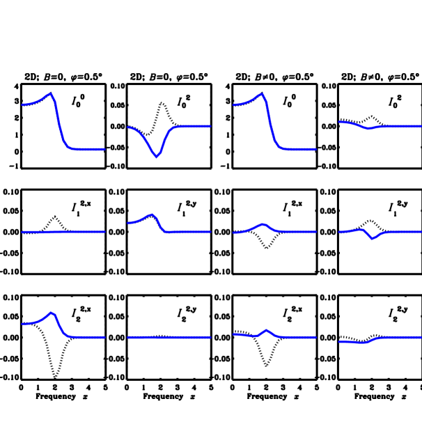
Figure 3: The emergent, surface averaged components of $\bm{\mathcal{I}}$ in non-magnetic (the first two columns) and magnetic (the last two columns) 2D media for $\mu=0.11$ and $\varphi=0.5^{\circ}$. The actual values of the components are scaled up by a factor of $10^{4}$. Solid and dotted lines represent respectively the AA and the AD PRD. In the first two columns (for $\bm{B}=0$), $I^{2,\rm x}_{1}$ and $I^{2,\rm y}_{2}$ are zero for the AA PRD (solid lines) and the other 10 components are non-zero (four AA components and six AD components). In the last two columns, the magnetic field parameters are $(\Gamma_{B},\theta_{B},\chi_{B})=(1,90^{\circ},60^{\circ})$. All the components are important for $\bm{B}\neq 0$.

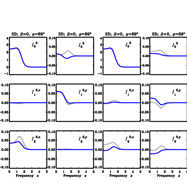
Figure 4: Same as Figure 3 but for $\varphi=89^{\circ}$.

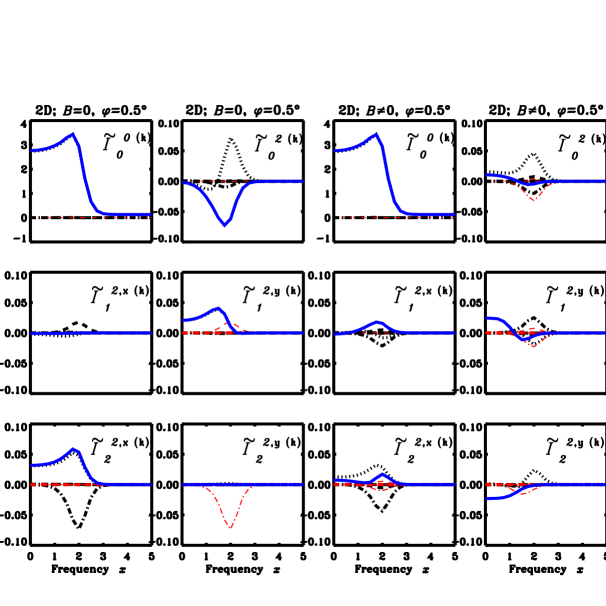
Figure 5: The emergent, spatially averaged components of $\tilde{\bm{\mathcal{I}}}^{(k)}$ in non-magnetic (the first two columns) and magnetic (the last two columns) 2D media for $\mu=0.11$ and $\varphi=89^{\circ}$. The actual values of the components are scaled up by a factor of $10^{4}$. Solid lines represent the components of $\bm{\mathcal{I}}$ for the AA PRD, plotted here for comparison. The dotted curves represent the components $\tilde{\bm{\mathcal{I}}}^{(0)}$. The thick curves with dashed, dot-dashed, dash-triple-dotted and long-dashed line types respectively represent ${\mathcal{R}e}\left[\tilde{\bm{\mathcal{I}}}^{(1)}\right]$, ${\mathcal{R}e}\left[\tilde{\bm{\mathcal{I}}}^{(2)}\right]$, ${\mathcal{R}e}\left[\tilde{\bm{\mathcal{I}}}^{(3)}\right]$ and ${\mathcal{R}e}\left[\tilde{\bm{\mathcal{I}}}^{(4)}\right]$. Similarly the thin curves with dashed, dot-dashed, dash-triple-dotted and long-dashed line types respectively represent ${\mathcal{I}m}\left[\tilde{\bm{\mathcal{I}}}^{(1)}\right]$, ${\mathcal{I}m}\left[\tilde{\bm{\mathcal{I}}}^{(2)}\right]$, ${\mathcal{I}m}\left[\tilde{\bm{\mathcal{I}}}^{(3)}\right]$ and ${\mathcal{I}m}\left[\tilde{\bm{\mathcal{I}}}^{(4)}\right]$. In the last two columns, the magnetic field parameters are $(\Gamma_{B},\theta_{B},\chi_{B})=(1,90^{\circ},60^{\circ})$.

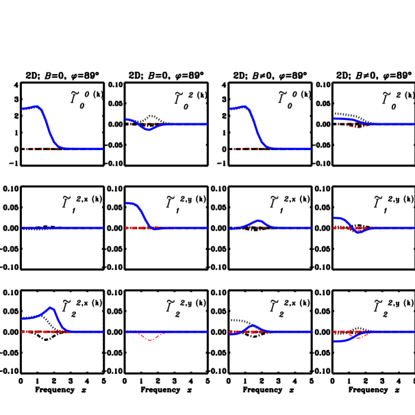
Figure 6: Same as Figure 5 but for $\varphi=89^{\circ}$.

In Figures 3 and 4, we plot the components of the real vector $\bm{\mathcal{I}}$=($I^{0}_{0}$, $I^{2}_{0}$, $I^{2,\rm x}_{1}$, $I^{2,\rm y}_{1}$, $I^{2,\rm x}_{2}$, $I^{2,\rm y}_{2}$) which are constructed using the 6 irreducible components of the nine vectors $\tilde{\bm{\mathcal{I}}}^{(0)}$, ${\mathcal{R}e}\left[\tilde{\bm{\mathcal{I}}}^{(1)}\right]$, ${\mathcal{I}m}\left[\tilde{\bm{\mathcal{I}}}^{(1)}\right]$, ${\mathcal{R}e}\left[\tilde{\bm{\mathcal{I}}}^{(2)}\right]$, ${\mathcal{I}m}\left[\tilde{\bm{\mathcal{I}}}^{(2)}\right]$, ${\mathcal{R}e}\left[\tilde{\bm{\mathcal{I}}}^{(3)}\right]$, ${\mathcal{I}m}\left[\tilde{\bm{\mathcal{I}}}^{(3)}\right]$, ${\mathcal{R}e}\left[\tilde{\bm{\mathcal{I}}}^{(4)}\right]$ and ${\mathcal{I}m}\left[\tilde{\bm{\mathcal{I}}}^{(4)}\right]$. For each $k$, $\tilde{\bm{\mathcal{I}}}^{(k)}$ is a 6-component complex vector ($\tilde{I}^{0\,(k)}_{0}$, $\tilde{I}^{2\,(k)}_{0}$, $\tilde{I}^{2,\rm x\,(k)}_{1}$, $\tilde{I}^{2,\rm y\,(k)}_{1}$, $\tilde{I}^{2,\rm x\,(k)}_{2}$, $\tilde{I}^{2,\rm y\,(k)}_{2}$). Thus in Figures 5 and 6 there are 54 components plotted in 6 panels, with each panel containing 9 curves (see the caption of Figure 5 for line identifications). In the Figures 3, 4, 5 and 6 the first two columns correspond to the $\bm{B}=0$ case and the last two columns correspond to the $\bm{B}\neq 0$ case. Here we have chosen $\mu=0.11$ and two examples of $\varphi$ namely $0.5^{\circ}$ and $89^{\circ}$. $\bm{\mathcal{I}}$ and $\tilde{\bm{\mathcal{I}}}^{(k)}$ are related through Equation (20) which can be re-written by truncating the Fourier series to five terms, as discussed and validated in Paper IV. Equation (20) can be approximated by

$$\bm{\mathcal{I}}\approx{\tilde{\bm{\mathcal{I}}}^{(0)}}+\sum_{k=1}^{k=4}2\,{\mathcal{R}e}\left[{\tilde{\bm{\mathcal{I}}}^{(k)}}\right],$$ (32)

for $\varphi=0.5^{\circ}$ and

$$\bm{\mathcal{I}}\approx{\tilde{\bm{\mathcal{I}}}^{(0)}}-2\,\Bigg{\{}{\mathcal{I}m}\left[\tilde{\bm{\mathcal{I}}}^{(1)}\right]+{\mathcal{R}e}\left[\tilde{\bm{\mathcal{I}}}^{(2)}\right]$$

$$-{\mathcal{I}m}\left[\tilde{\bm{\mathcal{I}}}^{(3)}\right]-{\mathcal{R}e}\left[\tilde{\bm{\mathcal{I}}}^{(4)}\right]\Bigg{\}},$$ (33)

for $\varphi=89^{\circ}$.

4.1.1 Non-magnetic case

In general the component $I^{0}_{0}$ (and hence Stokes $I$ parameter) is less sensitive to the AD nature of PRD functions. Only for certain choices of $(\theta,\varphi)$, does $[I^{0}_{0}]_{\rm AD}$ differ noticeably from $[I^{0}_{0}]_{\rm AA}$. The other polarization components exhibit significant sensitivity to the AD PRD. For the present choice of $(\theta,\varphi)$, in the second column of Figure 3 we see that $[I^{2,\rm y}_{1}]_{\rm AD}$ and $[I^{2,\rm y}_{1}]_{\rm AA}$ are nearly the same. We have verified that they differ very much for other choices of $(\theta,\varphi)$. Thus the differences between the AD PRD and the AA PRD are disclosed only when we consider polarization components and not just the $I^{0}_{0}$ component.

In the following we discuss the important symmetry relations of the polarized radiation field for a non-magnetic 2D medium.

Symmetry relations in non-magnetic 2D media In Paper II we have shown that $[I^{2,\rm x}_{1}]_{\rm AA}$ and $[I^{2,\rm y}_{2}]_{\rm AA}$ are identically zero in non-magnetic 2D media (shown as solid lines in the first two columns of Figures 3 and 4). This property of $I^{2,\rm x}_{1}$ and $I^{2,\rm y}_{2}$ in a non-magnetic 2D medium arises from the symmetry of the Stokes $I$ parameter with respect to the infinite axis of the medium ($X$-axis in our case), combined with the $\varphi$-dependence of the geometrical factors ${\mathcal{T}}^{K}_{Q}(i,\bm{\Omega})$ (see Appendix B of Paper II, Equations (B9) and (B10)). Such a symmetry property is valid if the scattering is according to CRD or the AA PRD where the angular dependence of the source vectors occurs only through the angular dependence of $(I,Q,U)$ and that of ${\mathcal{T}}^{K}_{Q}(i,\bm{\Omega})$. For the AD PRD, in addition to these two factors, the angle-dependence of the PRD functions also causes change in the angular behaviour of the source vectors. Thus the AD $r_{\rm II,III}$ functions depend on $\varphi$ in such a way that $[I^{2,\rm x}_{1}]_{\rm AD}$ and $[I^{2,\rm y}_{2}]_{\rm AD}$ are not zero in general (shown as dotted lines in the first two columns of Figures 3 and 4). Using a Fourier expansion of the AD $r_{\rm II,III}$ functions we have proved this fact in Appendix A.

The components of $\tilde{\bm{\mathcal{I}}}^{(k)}$ also exhibit some interesting properties. In Table 1 we list the dominant Fourier components contributing to each of the 6 components of $\bm{\mathcal{I}}$ in a non-magnetic 2D medium (shown as crosses). In the following we describe the nature of these Fourier components. Of all the components $\tilde{I}^{0(k)}_{0}$ and $\tilde{I}^{2(k)}_{0}$, only $\tilde{I}^{0(0)}_{0}$ and $\tilde{I}^{2(0)}_{0}$ (dotted lines in the first two columns of Figures 5 and 6) are dominant and they are nearly same as $[I^{0}_{0}]_{\rm AD}$ and $[I^{2}_{0}]_{\rm AD}$ respectively (dotted lines in the first two columns of Figures 3 and 4). $\tilde{I}^{2(0)}_{0}$ is an important ingredient for Stokes $Q$. The components $\tilde{I}^{2,{\rm x,y}(k)}_{1,2}$ are ingredients for both Stokes $Q$ and $U$. It can be seen that except $\tilde{I}^{2,{\rm y}(0)}_{2}$ all other $\tilde{I}^{2,{\rm x,y}(0)}_{1,2}$ play an important role in the construction of the vector $\bm{\mathcal{I}}$. For $\tilde{I}^{2,{\rm x}(k)}_{1,2}$, $k\neq 0$, only ${\mathcal{R}e}\left[\tilde{I}^{2,{\rm x}(1)}_{1}\right]$ and ${\mathcal{R}e}\left[\tilde{I}^{2,{\rm x}(2)}_{2}\right]$ (thick dashed and thick dot-dashed lines respectively) are dominant. For $\tilde{I}^{2,{\rm y}(k)}_{1,2}$, $k\neq 0$, only ${\mathcal{I}m}\left[\tilde{I}^{2,{\rm y}(1)}_{1}\right]$ and ${\mathcal{I}m}\left[\tilde{I}^{2,{\rm y}(2)}_{2}\right]$ (thin dashed and thin dot-dashed lines respectively) are dominant. This property is true for other choices of $(\theta,\varphi)$ also. From this property it appears that, in rapid computations involving the AD PRD mechanisms, it may prove useful to approximate the problem by using the truncated, 9-component vector ($\tilde{I}^{0(0)}_{0}$, $\tilde{I}^{2(0)}_{0}$, $\tilde{I}^{2,\rm x(0)}_{1}$, $\tilde{I}^{2,\rm y(0)}_{1}$, ${\mathcal{R}e}\left[\tilde{I}^{2,{\rm x}(1)}_{1}\right]$, ${\mathcal{I}m}\left[\tilde{I}^{2,{\rm y}(1)}_{1}\right]$, ${\mathcal{R}e}\left[\tilde{I}^{2,{\rm x}(2)}_{2}\right]$, ${\mathcal{I}m}\left[\tilde{I}^{2,{\rm y}(2)}_{2}\right]$) and obtain sufficiently accurate solution with less computational efforts. When the 6-component complex vector $\tilde{\bm{\mathcal{I}}}^{(k)}$ for each value of $k=0,1,2,3,4$, having 54 independent components is used, the computations are expensive.

4.1.2 Magnetic case

When we introduce a non-zero magnetic field $\bm{B}$, the shapes, signs and magnitudes of $\bm{\mathcal{I}}_{\rm AA,AD}$ change (see the last two columns of Figures 3 and 4). $[I^{2,\rm x}_{1}]_{\rm AA}$ and $[I^{2,\rm y}_{2}]_{\rm AA}$ which were zero when $\bm{B}=0$, now take non-zero values. With a given $\bm{B}\neq 0$, except $I^{0}_{0}$, the behaviors of all the other components for the AD PRD are very different from those for the AA PRD. Because the Hanle effect is operative only in the line core $(0\leq x\leq 3.5)$, all the magnetic effects are confined to the line core.

For $\bm{B}=0$ only some of the components of $\tilde{\bm{\mathcal{I}}}^{(k)}$ play a significant role. For $\bm{B}\neq 0$, all the components of $\tilde{\bm{\mathcal{I}}}^{(k)}$ can become important (see the last two columns of Figures 5 and 6). This property has a direct impact on the values of $Q/I$ and $U/I$.

4.2 Emergent Stokes Profiles

In Figures 7 and 8 we present the emergent, spatially averaged $Q/I$ and $U/I$ profiles computed using the AD and the AA PRD in line scattering for non-magnetic and magnetic 2D media. We show the results for $\mu=0.11$ and sixteen different values of $\varphi$ (marked on the respective panels). For the optically thin cases considered in this paper the AD PRD effects are restricted to the frequency domain $0\leq x\leq 5$. To understand these results let us consider two examples ($\varphi=0.5^{\circ}$ and 89^∘). For $\varphi=0.5^{\circ}$ we can approximate the emergent $Q$ and $U$ using Equations (3) and (4) as

$$Q(\mu=0.11,\varphi=0.5^{\circ},x)\approx$$

$$-\frac{3}{2\sqrt{2}}I^{2}_{0}-\frac{\sqrt{3}}{2}I^{2,\rm x}_{2},$$ (34)

and

$$U(\mu=0.11,\varphi=0.5^{\circ},x)\approx{\sqrt{3}}\,I^{2,\rm y}_{1}.$$ (35)

For $\varphi$=89^∘ also we can obtain approximate expressions for $Q$ and $U$ given by

$$Q(\mu=0.11,\varphi=89^{\circ},x)\approx$$

$$-\frac{3}{2\sqrt{2}}I^{2}_{0}+\frac{\sqrt{3}}{2}I^{2,\rm x}_{2},$$ (36)

and

$$U(\mu=0.11,\varphi=89^{\circ},x)\approx{\sqrt{3}}\,I^{2,\rm x}_{1}.$$ (37)

4.2.1 Angle-dependent PRD effects in the non-magnetic case

In both the Figures 7 and 8, the solid and dotted curves represent the $\bm{B}=0$ case. It is easy to observe that the differences between these curves depend on the choice of the azimuth angles $\varphi$ for $Q/I$, while for $U/I$ the differences are marginal.

The $Q/I$ profiles For $\varphi=0.5^{\circ}$ the $[Q/I]_{\rm AD}$ and $[Q/I]_{\rm AA}$ nearly coincide. But for $\varphi=89^{\circ}$ they differ by $\sim 1\%$ (in the degree of linear polarization) around $x=2$, which is very significant. From Equations (34) and (36) it is clear that $[Q/I]_{\rm AD}$ and $[Q/I]_{\rm AA}$ are controlled by the combinations of the components $I^{2}_{0}$ and $I^{2,\rm x}_{2}$. We can see from the first two columns of Figure 3 that for $\varphi=0.5^{\circ}$, $I^{2}_{0}$ and $I^{2,\rm x}_{2}$ have comparable magnitudes for both the AA and the AD PRD. Further, $[I^{2}_{0}]_{\rm AA}<0$, $[I^{2,\rm x}_{2}]_{\rm AA}>0$, $[I^{2}_{0}]_{\rm AD}>0$ and $[I^{2,\rm x}_{2}]_{\rm AD}<0$. From Equation (34) we can see that in spite of their opposite signs, because of their comparable magnitudes, the combinations of $I^{2}_{0}$ and $I^{2,\rm x}_{2}$ result in nearly same values of $[Q/I]_{\rm AD}$ and $[Q/I]_{\rm AA}$. When $\varphi=89^{\circ}$ the components $[I^{2}_{0}]_{\rm AA}$, $[I^{2}_{0}]_{\rm AD}$, $[I^{2,\rm x}_{2}]_{\rm AA}$ and $[I^{2,\rm x}_{2}]_{\rm AD}$ are of comparable magnitudes. Whereas $[I^{2}_{0}]_{\rm AA}$ and $[I^{2,\rm x}_{2}]_{\rm AA}$ have opposite signs, $[I^{2}_{0}]_{\rm AD}$ and $[I^{2,\rm x}_{2}]_{\rm AD}$ have the same sign. Therefore from Equation (36) we see that $[Q/I]_{\rm AD}$ differs from $[Q/I]_{\rm AA}$ for $\varphi=89^{\circ}$.

To understand the behaviors of the components of $I^{2}_{0}$ and $I^{2,\rm x}_{2}$ discussed above, we can refer to Figures 5, 6 and Table 1. The component $\tilde{I}^{2(0)}_{0}$ contributes dominantly to $I^{2}_{0}$, and is almost identical to $I^{2}_{0}$ because the contribution from $\tilde{I}^{2(k)}_{0}$ with $k=1,2,3,4$ are negligible (for both the values of $\varphi$). When $\varphi=0.5^{\circ}$, apart from $\tilde{I}^{2,\rm x\,(0)}_{2}$, the component ${\mathcal{R}e}\left[\tilde{I}^{2,\rm x\,(2)}_{2}\right]$ makes a significant contribution to $I^{2,\rm x}_{2}$ and $\tilde{I}^{2,\rm x\,(k)}_{2}$ with other values of $k$ vanish (graphically). ${\mathcal{R}e}\left[\tilde{I}^{2,\rm x\,(2)}_{2}\right]$ makes nearly equal and opposite contribution as $\tilde{I}^{2,\rm x\,(0)}_{2}$ when $\varphi=0.5^{\circ}$. When $\varphi=89^{\circ}$, the contribution of $\tilde{I}^{2,\rm x\,(0)}_{2}$ is larger than that of ${\mathcal{R}e}\left[\tilde{I}^{2,\rm x\,(2)}_{2}\right]$. Also, the components $\tilde{I}^{2\,(0)}_{0}$ and $\tilde{I}^{2,\rm x\,(0)}_{2}$ have the same sign for both the values of $\varphi$. Therefore From Equations (32) and (33) we can see that $I^{2}_{0}$ and $I^{2,\rm x}_{2}$ have opposite signs for $\varphi=0.5^{\circ}$ but have the same signs for $\varphi=89^{\circ}$.

The AD and the AA values of $Q/I$ sometimes coincide well and sometimes differ significantly. This is because, the Fourier components of the AD PRD functions $\tilde{r}^{(k)}_{\rm II,III}$ with $k=0$ essentially represent the azimuthal averages of the AD $r_{\rm II,III}$ functions and are not same as the explicit angle-averages of the AD $r_{\rm II,III}$ functions. The latter are obtained by averaging over both co-latitudes and azimuths (i.e., over all the scattering angles). The $\mu$-dependence of the AD $r_{\rm II,III}$ functions are contained dominantly in the $\tilde{r}^{(0)}_{\rm II,III}$ terms and the $\varphi$-dependence is contained dominantly in the higher order terms in the Fourier expansions of the AD $r_{\rm II,III}$ functions. For this reason the AA PRD cannot always be a good representation of the AD PRD, especially in the 2D polarized line transfer. This can be attributed to the strong dependence of the radiation field on the azimuth angle ($\varphi$) in the 2D geometry. As will be shown below, the differences between the AD and the AA solutions get further enhanced in the magnetic case (Hanle effect).

The $U/I$ profiles When $\bm{B}=0$, $[U/I]_{\rm AD}$ and $[U/I]_{\rm AA}$ profiles for both values of $\varphi$ (0.5^∘ and 89^∘) do not differ significantly. Equations (35) and (37) suggest that $U$ has dominant contribution from $I^{2,{\rm y}}_{1}$ for $\varphi$=0.5^∘ and $I^{2,{\rm x}}_{1}$ for 89^∘. Looking at the first two columns of Figure 5, it can be seen that $\tilde{I}^{2,\rm y\,(0)}_{1}$ nearly coincide with $[I^{2,\rm y}_{1}]_{\rm AA}$ for $\varphi=0.5^{\circ}$. Except $\tilde{I}^{2,\rm y\,(0)}_{1}$, $\tilde{I}^{2,\rm y\,(k)}_{1}$ for $k\neq 0$ make smaller contribution in the construction of $[I^{2,\rm y}_{1}]_{\rm AD}$. Thus $[I^{2,{\rm y}}_{1}]_{\rm AA}$ and $[I^{2,{\rm y}}_{1}]_{\rm AD}$ nearly coincide for $\varphi$=0.5^∘ (see the first two columns of Figure 3). Thus $[U/I]_{\rm AD}$ and $[U/I]_{\rm AA}$ are nearly the same for $\varphi$=0.5^∘. When $\varphi$=89^∘ (the first two columns of Figure 4), $[I^{2,{\rm x}}_{1}]_{\rm AA}$ vanishes. For each $k$, $\tilde{I}^{2,\rm x(k)}_{1}$ approach zero, as does $[I^{2,\rm x}_{1}]_{\rm AD}$, which is a combination of $\tilde{I}^{2,\rm x(k)}_{1}$. Thus $[U/I]_{\rm AD}$ and $[U/I]_{\rm AA}$ both are nearly zero for $\varphi$=89^∘. We can carry out similar analysis and find out which are the irreducible Fourier components of $\tilde{\bm{\mathcal{I}}}^{(k)}$ that contribute to the construction of $\bm{\mathcal{I}}$ and which of the components of $\bm{\mathcal{I}}$ contribute to generate $Q$ and $U$ to interpret their behaviors.

4.2.2 Angle-dependent PRD effects in the magnetic case

The presence of a weak, oriented magnetic field modifies the values of $Q/I$ and $U/I$ in the line core ($x\leq 3.5$) to a considerable extent, due to Hanle effect. Further, it is for $\bm{B}\neq 0$ that the differences between the AA and the AD PRD become more significant. In both the Figures 7 and 8, the dashed and dot-dashed curves represent $\bm{B}\neq 0$ case. As usual, there is either a depolarization (decrease in the magnitude) or a re-polarization (increase in the magnitude) of both $Q/I$ and $U/I$ with respect to those in the $\bm{B}=0$ case. The AD PRD values of $Q/I$ and $U/I$ are larger in magnitude (absolute values) than those of the AA PRD, for the chosen set of model parameters (this is not to be taken as a general conclusion). The differences depend sensitively on the value of $\bm{B}$.

Comparison with 1D results In Figures 9(a) and (b) we present the emergent $(I,Q/I,U/I)$ profiles for 1D and 2D media for $\mu=0.11$ and $\varphi=89^{\circ}$. For 2D RT, we present the spatially averaged profiles. The effects of a multi-D geometry (2D or 3D) on linear polarization for non-magnetic and magnetic cases are discussed in detail in Papers I, II and III, where we considered polarized line formation in multi-D media, scattering according to the AA PRD. We recall here that the essential effects are due to the finite boundaries in multi-D media, which cause leaking of radiation and hence a decrease in the values of Stokes $I$, and a sharp rise in the values of $Q/I$ and $U/I$ near the boundaries. Multi-D geometry naturally breaks the axisymmetry of the medium that prevails in a 1D planar medium. This leads to significant differences in the values of $Q/I$ and $U/I$ formed in 1D and multi-D media (compare solid lines in panels (a) and (b) of Figure  9). As pointed out in Papers I, II and III, for non-magnetic case, $U/I$ is zero in 1D media while in 2D media a non-zero $U/I$ is generated due to symmetry breaking by the finite boundaries. For the $(\theta,\varphi)$ values chosen in Figure 9(b) $[U/I]_{\rm AA}$is nearly zero even for non-magnetic 2D case, which is not generally true for other choices of $(\theta,\varphi)$ (see solid lines in various panels of Figure 8).

The effects of the AD PRD in $Q/I$ and $U/I$ profiles are already discussed above for non-magnetic and magnetic 2D media. They are similar for both 1D and 2D cases. For the non-magnetic 2D media, we can see the AD PRD effects even in $U/I$, which is absent in the corresponding 1D media. In 1D, one has to apply a non-zero magnetic field $\bm{B}$ in order to see the effects of the AD PRD on $U/I$ profiles.

The magnitudes of $[Q/I]_{\rm 1D}$ in the non-magnetic case and of $[Q/I]_{\rm 1D}$, $[U/I]_{\rm 1D}$ in the magnetic case are larger in comparison with the corresponding spatially averaged $[Q/I]_{\rm 2D}$ and $[U/I]_{\rm 2D}$. This is again due to leaking of photons from the finite boundaries and the effect of spatial averaging (which causes cancellation of positive and negative quantities).

4.3 Radiation anisotropy in 2D media–Stokes source vectors

In Figures 10 and 11 we present spatial distribution of $S_{I}$, $S_{Q}$ and $S_{U}$ on the plane of the 2D slab for two different frequencies ($x=0$ and $x=2.5$ respectively). The spatial distribution of source vector components $S_{Q}$ and $S_{U}$ represent the anisotropy of the radiation field in the 2D medium. It shows how inhomogeneous is the distribution of linear polarization within the 2D medium.

In Figure 10 we consider $x=0$ (line center). For the chosen values of $(\theta,\varphi)$ the spatial distribution of $S_{I}$ is not very different for the AA and the AD PRD. $S_{Q}$ and $S_{U}$ for both the AA and the AD PRD have similar magnitudes (Figures 10(b),(c) and 10(e),(f)), but different spatial distributions. The spatial distribution of $S_{Q}$ and $S_{U}$ is such that the positive and negative contributions with similar magnitudes of $S_{Q}$ and $S_{U}$ cancel out in the computation of their formal integrals. Therefore, the average values of $Q/I$ and $U/I$ resulting from the formal integrals of $S_{Q}$ and $S_{U}$ are nearly zero at $x=0$ for both the AA and the AD PRD (see dashed and dot-dashed lines at $x=0$ in Figure 9(b)).

In Figure 11 we consider $x=2.5$ (near wing frequency). Again, $S_{I}$ does not show significant differences between the AA and the AD PRD. For $S_{Q}$, the AA PRD has a distribution with positive and negative values equally distributed in the 2D slab but the AD PRD has more negative contribution. This reflects in the average values of $Q/I$, where $[Q/I]_{\rm AA}$ approach zero due to cancellation, while $[Q/I]_{\rm AD}$ values are more negative (see dashed and dot-dashed lines at $x=2.5$ in Figure 9(b)). The positive and negative values of $S_{U}$ are distributed in a complicated manner everywhere on the 2D slab for the AA PRD. For the AD PRD, the distribution of $S_{U}$ is positive almost everywhere, including the central parts of the 2D slab. Such a spatial distribution reflects again in the average value of $U/I$ (shown in Figure 9(b)), where $[U/I]_{\rm AA}$ have smaller positive magnitudes (due to cancellation effects) than the corresponding $[U/I]_{\rm AD}$.

5 CONCLUSIONS

In this paper we have further generalized the Fourier decomposition technique developed in Paper IV to handle the AD PRD in multi-D polarized RT (see Section 2.2). We have applied this technique and developed an efficient iterative method called Pre-BiCG-STAB to solve this problem (see Section 3).

We prove in this paper that the symmetry of the polarized radiation field with respect to the infinite axis, that exists for a non-magnetic 2D medium for the AA PRD (as shown in Paper II) breaks down for the AD PRD (see Appendix A).

We present results of the very first investigations of the effects of the AD PRD on the polarized line formation in multi-D media. We restrict our attention to freestanding 2D slabs with finite optical thicknesses on the two axes ($Y$ and $Z$). The optical thicknesses of the isothermal 2D media considered in this paper are very moderate ($T=20$). We consider effects of the AD PRD on the scattering polarization in both non-magnetic and magnetic cases. We find that the relative AD PRD effects are prominent in the magnetic case (Hanle effect). They are also present in non-magnetic case for some choices of $(\theta,\varphi)$. We conclude that the AD PRD effects are important for interpreting the observations of scattering polarization in multi-D structures on the Sun.

Practically, even with the existing advanced computing facilities, it is extremely difficult to carryout the multi-D polarized RT with the AD PRD in spite of using advanced numerical techniques. Therefore in this paper we restrict our attention to isothermal 2D slabs. The use of the AD PRD in 3D polarized RT in realistic modeling of the observed scattering polarization on the Sun will be numerically very expensive and can be taken up in future only with highly advanced computing facilities.

Erratum:  In the previous papers of this series (Papers I, III and IV) the definitions of the formal solutions expressed in terms of the optical thicknesses have a notational error. In Equation (20) of Paper I, Equations (14) and (20) of Paper III, Equation (14) of Paper IV, the symbol $\tau_{x,\rm max}$ should have been $\tau_{x}(\bm{r},\bm{\Omega})$ as explicitly given in Equation (13) of this paper. $\tau_{x}(\bm{r},\bm{\Omega})$ is defined in Equation (14) in this paper. In the previous papers of this series (Papers I to IV) the vector $\bm{r}^{\prime}=\bm{r}-(s-s^{\prime})\bm{\Omega}$ was incorrectly defined as $\bm{r}-s^{\prime}\bm{\Omega}$. We note here that the numerical results and all other equations presented in Papers I – IV are correct, and are unaffected by this error in the above mentioned equations.

Appendix A SYMMETRY BREAKING PROPERTIES OF THE AD PRD FUNCTIONS IN NON-MAGNETIC 2D MEDIA

In this appendix we show that the symmetry properties that are valid for the AA PRD (proved in Paper II) break down for the AD PRD. We present the proof in the form of an algorithm.

Step (1):  First we assume that the medium contains only an unpolarized thermal source namely, $\bm{\mathcal{S}}=(\epsilon B(\bm{r}),0,0,0,0,0)^{T}$.

Step (2):  Use of this source vector in the formal solution expression yields $\bm{\mathcal{I}}=(I^{0}_{0},0,0,0,0,0)^{T}$.

Step 3:  Using this $\bm{\mathcal{I}}$ we can write the expressions for the irreducible polarized mean intensity components as

$$J^{0}_{0}(\bm{r},\bm{\Omega},x)\simeq\int_{x^{\prime},\bm{\Omega}^{\prime}}\frac{\hat{R}(x,x^{\prime},\bm{\Omega},\bm{\Omega^{\prime}})}{\phi(x)}\,I^{0}_{0}(\bm{r},\theta^{\prime},\varphi^{\prime},x^{\prime}),$$

$$J^{2}_{0}(\bm{r},\bm{\Omega},x)\simeq c_{2}\int_{x^{\prime},\bm{\Omega}^{\prime}}\frac{\hat{R}(x,x^{\prime},\bm{\Omega},\bm{\Omega}^{\prime})}{\phi(x)}(3\cos^{2}\theta^{\prime}-1)\,I^{0}_{0}(\bm{r},\theta^{\prime},\varphi^{\prime},x^{\prime}),$$

$$J^{\rm 2,x}_{1}(\bm{r},\bm{\Omega},x)\simeq-c_{3}\int_{x^{\prime},\bm{\Omega}^{\prime}}\frac{\hat{R}(x,x^{\prime},\bm{\Omega},\bm{\Omega}^{\prime})}{\phi(x)}\sin 2\theta^{\prime}\cos\varphi^{\prime}\,I^{0}_{0}(\bm{r},\theta^{\prime},\varphi^{\prime},x^{\prime}),$$

$$J^{\rm 2,y}_{1}(\bm{r},\bm{\Omega},x)\simeq c_{4}\int_{x^{\prime},\bm{\Omega}^{\prime}}\frac{\hat{R}(x,x^{\prime},\bm{\Omega},\bm{\Omega}^{\prime})}{\phi(x)}\sin 2\theta^{\prime}\sin\varphi^{\prime}\,I^{0}_{0}(\bm{r},\theta^{\prime},\varphi^{\prime},x^{\prime}),$$

$$J^{\rm 2,x}_{2}(\bm{r},\bm{\Omega},x)\simeq c_{5}\int_{x^{\prime},\bm{\Omega}^{\prime}}\frac{\hat{R}(x,x^{\prime},\bm{\Omega},\bm{\Omega}^{\prime})}{\phi(x)}\sin^{2}\theta^{\prime}\cos 2\varphi^{\prime}\,I^{0}_{0}(\bm{r},\theta^{\prime},\varphi^{\prime},x^{\prime}),$$

$$J^{\rm 2,y}_{2}(\bm{r},\bm{\Omega},x)\simeq-c_{6}\int_{x^{\prime},\bm{\Omega}^{\prime}}\frac{\hat{R}(x,x^{\prime},\bm{\Omega},\bm{\Omega}^{\prime})}{\phi(x)}\sin^{2}\theta^{\prime}\sin 2\varphi^{\prime}\,I^{0}_{0}(\bm{r},\theta^{\prime},\varphi^{\prime},x^{\prime}),$$

(A1)

where

$$\int_{x^{\prime},\bm{\Omega}^{\prime}}=\int_{-\infty}^{+\infty}dx^{\prime}\oint\frac{d\bm{\Omega}^{\prime}}{4\pi},$$ (A2)

and $c_{i},i=2,3,4,5,6$ are positive numbers (see appendix D of Paper III). We recall that ${\rm d}\bm{\Omega}^{\prime}=\sin\theta^{\prime}\,d\theta^{\prime}\,d\varphi^{\prime}$, $\theta^{\prime}\in[0,\pi]$ and $\varphi^{\prime}\in[0,2\pi]$. Here

$$\hat{R}(x,x^{\prime},\bm{\Omega},\bm{\Omega}^{\prime})=$$

$$\hat{W}\left[\hat{\alpha}r_{\rm II}(x,x^{\prime},\bm{\Omega},\bm{\Omega}^{\prime})+\left(\hat{\beta}-\hat{\alpha}\right)r_{\rm III}(x,x^{\prime},\bm{\Omega},\bm{\Omega}^{\prime})\right],$$ (A3)

is the non-magnetic, polarized redistribution matrix.

Step 4:  A Fourier expansion of the AD PRD functions with respect to $\varphi^{\prime}$ (instead of $\varphi$) gives

$$r_{\rm II,III}(x,x^{\prime},\bm{\Omega},\bm{\Omega^{\prime}})=$$

$$\sum_{k^{\prime}=0}^{k^{\prime}=\infty}\,\,(2-\delta_{k^{\prime}0})e^{ik^{\prime}\varphi^{\prime}}\,\,{\tilde{r}}_{\rm II,III}^{(k^{\prime})}(x,x^{\prime},\bm{\Omega},\theta^{\prime}),$$ (A4)

with the Fourier coefficients

$${\tilde{r}}^{(k)}(x,x^{\prime},\bm{\Omega},\theta^{\prime})=\int_{0}^{2\pi}\frac{d\,\varphi^{\prime}}{2\pi}\,e^{-ik^{\prime}\varphi^{\prime}}\,\,$$

$${r}_{\rm II,III}(x,x^{\prime},\bm{\Omega},\bm{\Omega^{\prime}}).$$

(A5)

Substituting Equation (A4) in Equation (A1) we can show that the components $J^{\rm 2,x}_{1}$ and $J^{\rm 2,y}_{2}$ do not vanish irrespective of the symmetry of $I^{0}_{0}$ with respect to the infinite spatial axis. In other words, to a first approximation, even if we assume that $I^{0}_{0}$ is symmetric with respect to the infinite spatial axis (as in the AA PRD), the $\varphi^{\prime}$-dependence of the AD PRD functions $r_{\rm II,III}$ is such that the integral over $\varphi^{\prime}$ leads to non-zero $J^{\rm 2,x}_{1}$ and $J^{\rm 2,y}_{2}$. This stems basically from the coefficients with $k^{\prime}\neq 0$ in the expansion of the AD PRD functions. Following an induction proof as in Paper II, it follows that $J^{\rm 2,x}_{1}$ and $J^{\rm 2,y}_{2}$ are non-zero in general because the symmetry breaks down in the first step itself.

It follows from Equation (2), and from the above proof that the Stokes $I$ parameter is not symmetric with respect to the infinite spatial axis in a non-magnetic 2D media, in the AD PRD case, unlike the AA PRD and CRD cases (see Appendix B of Paper II for the proof for the AA PRD).

Table 1: The dominant Fourier components contributing to each of the 6 irreducible components of $\bm{\mathcal{I}}$ in a non-magnetic 2D medium, shown as cross symbols.

	$k=0$	$k=1$	$k=2$	$k=3$	$k=4$
$\tilde{\mathcal{I}}^{0(k)}_{0}$	x	-	-	-	-
$\tilde{\mathcal{I}}^{2(k)}_{0}$	x	-	-	-	-
${\mathcal{R}e}\left[\tilde{\mathcal{I}}^{2,\rm x(k)}_{1}\right]$	x	x	-	-	-
${\mathcal{I}m}\left[\tilde{\mathcal{I}}^{2,\rm x(k)}_{1}\right]$	-	-	-	-	-
${\mathcal{R}e}\left[\tilde{\mathcal{I}}^{2,\rm y(k)}_{1}\right]$	x	-	-	-	-
${\mathcal{I}m}\left[\tilde{\mathcal{I}}^{2,\rm y(k)}_{1}\right]$	-	x	-	-	-
${\mathcal{R}e}\left[\tilde{\mathcal{I}}^{2,\rm x(k)}_{2}\right]$	x	-	x	-	-
${\mathcal{I}m}\left[\tilde{\mathcal{I}}^{2,\rm x(k)}_{2}\right]$	-	-	-	-	-
${\mathcal{R}e}\left[\tilde{\mathcal{I}}^{2,\rm y(k)}_{2}\right]$	-	-	-	-	-
${\mathcal{I}m}\left[\tilde{\mathcal{I}}^{2,\rm y(k)}_{2}\right]$	-	-	x	-	-

Figure 1: The definition of the spatial location $\bm{r}$ and the projected distances $(s-s^{\prime})\bm{\Omega}$ which appear in the 2D formal solution integral (Equation (12)). $\bm{r}_{0}$ and $\bm{r}$ are the initial and final locations considered in the formal solution integral. The values of the variable along the ray satisfy $s_{0}<s^{\prime}<s$.

Figure 2: RT in a 2D medium. We assume that the medium is infinite in the direction of the $X$-axis and has a finite dimension in the direction of the $Y$-axis and the $Z$-axis. The top surface is marked.

Figure 7: Emergent, spatially averaged $Q/I$ profiles for a 2D medium with $T_{Y}=T_{Z}=20$, for a line of sight $\mu=0.11$. Different panels correspond to different values of $\varphi$ marked in the panels. Solid and dotted lines correspond to the AA and the AD profiles for $\bm{B}=0$. Dashed and dot-dashed lines correspond to the AA and the AD profiles in a magnetic medium with magnetic field parameter $(\Gamma,\theta_{B},\chi_{B})=(1,90^{\circ},60^{\circ})$.

Figure 8: Same as Figure 7 but for $U/I$.

Figure 9: Panel (a) shows emergent $(I,Q/I,U/I)$ profiles formed in an 1D medium and the panel (b) shows the emergent, spatially averaged $(I,Q/I,U/I)$ profiles formed in a 2D medium. The solid and dotted lines represent respectively the AA and the AD profiles for $\bm{B}=0$. The dashed and dash-triple-dotted lines represent respectively the AA and the AD profiles for $\bm{B}\neq 0$, with the magnetic field parameterized by $(\Gamma,\theta_{B},\chi_{B})=(1,90^{\circ},60^{\circ})$. The results are shown for $\mu=0.11$ and $\varphi=89^{\circ}$. For the panel (a) we take $T_{Z}=T=20$ and for the panel (b), $T_{Z}=T_{Y}=T=20$.

Figure 10: Surface plots of $S_{I}$, $S_{Q}$ and $S_{U}$ for the AA (left panels) and the AD PRD (right panels) for $x=0$. The source vector components are plotted as a function of the grid indices along $Y$ and $Z$ directions. Here $\bm{B}\neq 0$, with $(\Gamma,\theta_{B},\chi_{B})=(1,90^{\circ},60^{\circ})$. The other model parameters are same as in Figure 9.

Figure 11: Same as Figure 10 for $x=2.5$.

References

• Anusha & Nagendra (2011a) Anusha, L. S., & Nagendra, K. N. 2011a, ApJ, 726, 6 (Paper I)
• Anusha & Nagendra (2011b) Anusha, L. S., & Nagendra, K. N. 2011b, ApJ, 738, 116 (Paper III)
• Anusha et al. (2011a) Anusha, L. S., Nagendra, K. N., & Paletou, F. ApJ, 2011a, 726, 96 (Paper II)
• Anusha et al. (2011b) Anusha, L. S., Nagendra, K. N., Bianda, M., Stenflo, J. O., Holzreuter, R., Sampoorna, M., Frisch, H., Ramelli, R. & Smitha, H. N., 2011b, ApJ, 737, 95
• Anusha & Nagendra (2011c) Anusha, L. S., & Nagendra, K. N. 2011c, ApJ, 739, 40 (Paper IV)
• Bommier (1997a) Bommier, V. 1997a, A&A, 328, 706
• Bommier (1997b) Bommier, V. 1997b, A&A, 328, 726
• Chandrasekhar (1960) Chandrasekhar, S. 1960, Radiative Transfer (New York: Dover)
• Faurobert-Scholl (1992) Faurobert-Scholl, M. 1992, A&A, 258, 521
• Frisch (2007) Frisch, H. 2007, A&A, 476, 665 (HF07)
• Frisch (2009) Frisch, H. 2009, in ASP Conf. Ser. 405, Solar Polarization 5, ed. S. V. Berdyugina, K. N. Nagendra & R. Ramelli (San Francisco: ASP), 87 (HF09)
• Hummer (1962) Hummer, D. G. 1962, MNRAS, 125, 21
• Landi Degl’Innocenti & Landolfi (2004) Landi Degl’Innocenti, E., & Landolfi, M. 2004, Polarization in Spectral Lines (Dordrecht: Kluwer)
• Nagendra et al. (2002) Nagendra, K. N., Frisch, H., & Faurobert, M. 2002, A&A, 395, 305
• Nagendra & Sampoorna (2011) Nagendra, K. N., & Sampoorna, M., 2011, A&A(in press)
• Saad (2000) Saad, Y. 2000, Iterative methods for Sparse Linear Systems (2nd ed.) (ebook:http://www-users.cs.umn.edu/ saad/books.html)