Multi-dimensional radiative transfer to analyze Hanle effect in Ca ii K line at 3933 Å 

Abstract

Radiative transfer (RT) studies of the linearly polarized spectrum of the Sun (the second solar spectrum) have generally focused on the line formation, with an aim to understand the vertical structure of the solar atmosphere using one-dimensional (1D) model atmospheres. Modeling spatial structuring in the observations of the linearly polarized line profiles requires the solution of multi-dimensional (multi-D) polarized RT equation and a model solar atmosphere obtained by magneto-hydrodynamical (MHD) simulations of the solar atmosphere. Our aim in this paper is to analyze the chromospheric resonance line Ca ii K at 3933 Å using multi-D polarized RT with Hanle effect and partial frequency redistribution in line scattering. We use an atmosphere which is constructed by a two-dimensional snapshot of the three-dimensional MHD simulations of the solar photosphere, combined with columns of an 1D atmosphere in the chromosphere. This paper represents the first application of polarized multi-D RT to explore the chromospheric lines using multi-D MHD atmospheres, with PRD as the line scattering mechanism. We find that the horizontal inhomogeneities caused by MHD in the lower layers of the atmosphere are responsible for strong spatial inhomogeneities in the wings of the linear polarization profiles, while the use of horizontally homogeneous chromosphere (FALC) produces spatially homogeneous linear polarization in the line core. Introduction of different magnetic field configurations modifies the line core polarization through Hanle effect and can cause spatial inhomogeneities in the line core. A comparison of our theoretical profiles with the observations of this line shows that the MHD structuring in the photosphere is sufficient to reproduce the line wings and in the line core, only line center polarization can be reproduced using Hanle effect. For a simultaneous modeling of the line wings and the line core (including the line center), MHD atmospheres with inhomogeneities in the chromosphere are required.

1 INTRODUCTION

Scattering polarization in strong resonance lines such as Ca i 4227 Å  and Ca ii K at 3933 Å  can be used to diagnose the chromospheric magnetic fields (see e.g., Faurobert-Scholl, 1992; Holzreuter et al., 2005; Sampoorna et al., 2009; Anusha et al., 2010, 2011b; Frisch et al., 2012) and also to explore the temperature bifurcation in the chromosphere (Holzreuter et al., 2006; Holzreuter & Stenflo, 2007a, b). All these studies consider one-dimensional (1D) models of the solar atmosphere such as FALC (Fontenla et al., 1993). However the solar atmosphere is extremely inhomogeneous to be well represented by 1D stratification of the physical quantities. Observations using ZIMPOL (Gandorfer et al., 2004) show strong spatial variation of the linear polarization along the slit, indicating spatial structuring in the atmosphere (see e.g., Bianda et al., 2003; Stenflo, 2006; Sampoorna et al., 2009). A natural explanation of this spatial structuring in the line core is in terms of Hanle effect from spatially varying magnetic fields. The spatial distribution of linear polarization, both in the core and the wings is caused by the local departures from axial symmetry of the atmosphere. In the line core, this effect is entangled with the effect of spatially varying magnetic fields (see Stenflo, 2006). To model such observations one has to solve multi-dimensional (multi-D) polarized radiative transfer (RT) equation with Hanle effect and partial frequency redistribution (PRD) in line scattering. Methods have been developed to solve this problem in a series of papers (Anusha & Nagendra, 2011a; Anusha et al., 2011a; Anusha & Nagendra, 2011b, c, d). In these papers we used isothermal atmospheres and hypothetical lines for the sake of simplicity and to establish the relevant RT equation and its solution. In the present paper we apply the methods developed in the above series of papers to the case of Ca ii K line at 3933 Å .

Construction of MHD solar atmospheres achieved considerable success to represent the ‘solar photosphere’ (see e.g., Nordlund & Stein, 1991; Vögler et al., 2005, and references cited therein). Such photospheric models have been used to analyze photospheric lines such as Sr i 4607 Å  using polarized three-dimensional (3D) RT equation and assuming complete frequency redistribution (CRD) (see e.g., Trujillo Bueno et al., 2004; Trujillo Bueno & Shchukina, 2007; Shchukina & Trujillo Bueno, 2007, and references cited therein). However constructing MHD models that very well represent the ‘solar chromosphere’ remains still a challenging problem. A detailed review on the MHD and RT in 3D model atmospheres can be found in Carlsson (2009).

In this paper we consider a 2D model, which is a combination of a vertical slice through the MHD snapshot from Nordlund & Stein (1991) and the 1D hydrostatic FALC model, replicated horizontally and joined smoothly in the vertical direction (provided by Han Uitenbroek, through a private communication). This atmosphere does not have any horizontal inhomogeneities in the chromospheric layers. Hereafter we call this atmosphere as MHD-FALC model atmosphere. This atmosphere may not quite well represent the reality, but it certainly acts as an intermediate step between the existing 1D models and the real multi-D MHD chromospheric atmospheres, the research on which is not established yet. Using this atmosphere we study the synthetic linear polarization profiles of Ca ii K line at 3933 Å .

In Section 2 we give all the governing equations of the problem. In Section 3 we provide the mathematical background of the solution method. In Section 3.2 we provide important numerical details. Section 4 is devoted to a discussion on the spatial dependence of some crucial physical parameters. In Section 5 we discuss the contribution functions. In Section 6 we discuss the results of our studies. Section 7 is devoted to the conclusions. In Appendix A we give some mathematical details of the methods used in this paper.

2 FORMULATION OF THE PROBLEM

For the line under consideration we first solve the unpolarized non-LTE multi-level RT equation and statistical equilibrium equation simultaneously and iteratively, using the code of Uitenbroek (2000, 2001, 2006) (the RH-code). This code uses the Multi-level Accelerated Lambda Iteration (MALI) scheme of Rybicki & Hummer (1991, 1992). We consider 6 energy levels with 5 line transitions and 5 continuum transitions. The main lines at 3933 Å  and 3968 Å  are treated in PRD and other lines in CRD. From the RH-code, we obtain level populations, radiative and collisional rates, opacities, and also the center to limb variation of the unpolarized intensity profiles. Keeping these quantities fixed, we then solve the polarized two-level RT equation for the main line under consideration. We use sophisticated domain based PRD theory formulated by Bommier (1997a, b) (particularly the approximation level III). We start with the unpolarized source function as an initial solution, and use the Stabilized Preconditioned BiConjugate Gradient (Pre-BiCG-STAB) technique (see Anusha et al., 2009, 2011a; Anusha & Nagendra, 2011b). We work with the irreducible spherical tensor formulation of multi-D RT developed in Anusha & Nagendra (2011a, b). The 2D short-characteristics formal solution is used (see Auer & Paletou, 1994; Kunasz & Auer, 1988).

The 3D MHD atmospheres are cuboids with all the physical parameters depending on the spatial variables $x$, $y$ and $z$. In MHD-FALC model we consider a 2D snapshot along $Y$ direction so that in our calculations we have the physical parameters dependent only on $x$ and $z$ (see Figure 1). We assume a periodic 2D medium with periodic horizontal boundary conditions. For a ray traveling in the direction $\bm{\Omega}$ the 2D RT equation at a point $\bm{r}=(x,z)$ in the Cartesian co-ordinate system is given by

$$\bm{\Omega}\cdot\nabla\bm{I}(\lambda,\bm{\Omega},\bm{r})=$$

$$-[\kappa_{\rm tot}(\lambda,\bm{r})]\left[\bm{I}(\lambda,\bm{\Omega},\bm{r})-\bm{S}(\lambda,\bm{\Omega},\bm{r})\right],$$ (1)

where $\bm{I}$ = $(I,Q,U)^{T}$ is the Stokes vector and $\bm{S}=(S_{I},S_{Q},S_{U})^{T}$ is the source vector. The ray direction is defined by $\bm{\Omega}=(\theta,\varphi)$ where $\theta$ and $\varphi$ denote the inclination and the azimuth of the scattered ray. The direction cosines of the ray are $(\sin\theta\,\cos\varphi\,,\sin\theta\,\sin\varphi\,,\cos\theta)$ =$(\gamma,\eta,\mu)$. The total opacity is

$$\kappa_{\rm tot}(\lambda,\bm{r})=[\kappa_{l}(\bm{r})\phi(\lambda,\bm{r})+\kappa_{c}(\lambda,\bm{r})+\sigma_{c}(\lambda,\bm{r})].$$ (2)

Here $\kappa_{l}$, $\kappa_{c}$ and $\sigma_{c}$ are wavelength averaged line opacity, continuum absorption and continuum scattering coefficients respectively. $\phi$ is the normalized Voigt profile function. The profile function depends on $\bm{r}$ through the damping parameter $a$ which depends on the radiative de-excitation rate $\Gamma_{R}$, elastic and inelastic collision rates $\Gamma_{E}$ and $\Gamma_{I}$ respectively and the Doppler width $\Delta\nu_{D}$ so that

$$a=\frac{\Gamma_{R}+\Gamma_{E}+\Gamma_{I}}{4\pi\Delta\nu_{D}}.$$ (3)

For the Ca ii K line at 3933 Å  $\Gamma_{R}=1.5\times 10^{8}s^{-1}$. $\Gamma_{E}$ is computed taking into account the van der Waal’s broadening (arising due to elastic collisions with neutral hydrogen) and Stark broadening (arising due to interactions with free electrons). $\Gamma_{I}$ includes the inelastic collision processes like collisional de-excitation by electrons and protons, collisional ionization by electrons, and charge exchange processes (see Uitenbroek, 2001). Here $\Delta\nu_{D}=\sqrt{{2k_{B}T}/{M_{a}}+v^{2}_{turb}}/\lambda_{0}$, with $k_{B}$ the Boltzmann constant, $T$ the temperature, $M_{a}$ the mass of the atom, $v_{turb}$ the micro-turbulent velocity (taken as 1 km/s), and $\lambda_{0}$ the line center wavelength. In a two-level model atom with unpolarized ground level, the total source vector $\bm{S}$ is defined as

$$\bm{S}(\lambda,\bm{\Omega},\bm{r})=\frac{\kappa_{l}(\bm{r})\phi(\lambda,\bm{r})\bm{S}_{l}(\lambda,\bm{\Omega},\bm{r})}{\kappa_{\rm tot}(\lambda,\bm{r})}$$

$$+\frac{\sigma_{c}(\lambda,\bm{r})\bm{S}_{c}(\lambda,\bm{\Omega},\bm{r})+\kappa_{c}(\lambda,\bm{r}){B}_{\lambda}(\bm{r}){\bm{U}}}{\kappa_{\rm tot}(\lambda,\bm{r})}.$$

(4)

Here $\bm{U}=(1,0,0)^{T}$ and $B_{\lambda}$ is the Planck function. The line source vector is

$${\bm{S}}_{l}(\lambda,\bm{\Omega},\bm{r})=\epsilon{B}_{\lambda}(\bm{r})\bm{U}$$

$$\!\!\!\!\!\!\!\!\!\!+\int_{-\infty}^{+\infty}\oint\frac{\hat{R}(\lambda,\lambda^{\prime},\bm{\Omega},\bm{\Omega}^{\prime},\bm{r},\bm{B})}{\phi(x)}$$

$$\times\,{\bm{I}}(\lambda^{\prime},\bm{\Omega}^{\prime},\bm{r})\,\frac{d\bm{\Omega}^{\prime}}{4\pi}\,d\lambda^{\prime}.$$ (5)

Here $\hat{R}$ is the Hanle redistribution matrix (Bommier, 1997a, b). $\bm{B}$ is the vector magnetic field taken to be a free parameter. The continuum scattering source vector is

$${\bm{S}}_{c}(\lambda,\bm{\Omega},\bm{r})=\oint\hat{P}(\bm{\Omega},\bm{\Omega}^{\prime}){\bm{I}}(\lambda,\bm{\Omega}^{\prime},\bm{r})\,\frac{d\bm{\Omega}^{\prime}}{4\pi},$$ (6)

where $\hat{P}$ is the Rayleigh scattering phase matrix (Chandrasekhar, 1960). For simplicity, frequency coherent scattering is assumed for the continuum. The thermalization parameter $\epsilon$ is defined by $\epsilon={\Gamma_{I}}/(\Gamma_{R}+\Gamma_{I})$. ($\lambda^{\prime}$, $\bm{\Omega}^{\prime}$) and ($\lambda$, $\bm{\Omega}$) in Equation (5) refer to the wavelength and direction of the incoming and the outgoing rays, respectively.

3 METHOD OF SOLUTION

In Anusha & Nagendra (2011a, b) we describe a method of decomposing the Stokes vectors and Stokes source vectors into irreducible spherical tensors ${\mathcal{T}}^{K}_{Q}$ (see e.g., Landi Degl’Innocenti & Landolfi, 2004) which transforms the multi-D RT equation into a simpler form that can be solved using any iterative method (see Section 3.1). In Anusha et al. (2011a) and Anusha & Nagendra (2011b) we develop a fast iterative method called the Pre-BiCG-STAB for polarized multi-D RT with PRD. We use both these techniques here to solve the relevant RT equation. Because of the use of continuum scattering the algorithm for the Pre-BiCG-STAB should be modified slightly, which is described in Appendix A.

3.1 Irreducible spherical tensors for multi-D RT

Using irreducible spherical tensors we can represent the linearly polarized radiation field through a six component vector denoted by $\bm{\mathcal{I}}=(I^{0}_{0},I^{2}_{0},I^{2,x}_{1},I^{2,y}_{1},I^{2,x}_{2},I^{2,y}_{2})^{T}$ which are related to the Stokes parameters $I,Q$ and $U$ through the following expressions (see Frisch, 2007).

$$I(\lambda,\bm{\Omega},\bm{r})=I^{0}_{0}+\frac{1}{2\sqrt{2}}(3\cos^{2}\theta-1)I^{2}_{0}$$

$$-\sqrt{3}\cos\theta\sin\theta(I^{2,x}_{1}\cos\varphi-I^{2,y}_{1}\sin\varphi)$$

$$+\frac{\sqrt{3}}{2}(1-\cos^{2}\theta)(I^{2,x}_{2}\cos 2\varphi-I^{2,y}_{2}\sin 2\varphi),$$

(7)

$$Q(\lambda,\bm{\Omega},\bm{r})=-\frac{3}{2\sqrt{2}}(1-\cos^{2}\theta)I^{2}_{0}$$

$$-\sqrt{3}\cos\theta\sin\theta(I^{2,x}_{1}\cos\varphi-I^{2,y}_{1}\sin\varphi)$$

$$-\frac{\sqrt{3}}{2}(1+\cos^{2}\theta)(I^{2,x}_{2}\cos 2\varphi-I^{2,y}_{2}\sin 2\varphi),$$

(8)

$$U(\lambda,\bm{\Omega},\bm{r})=\sqrt{3}\sin\theta(I^{2,x}_{1}\sin\varphi+I^{2,y}_{1}\cos\varphi)$$

$$+\sqrt{3}\cos\theta(I^{2,x}_{2}\sin 2\varphi+I^{2,y}_{2}\cos 2\varphi).$$ (9)

Here $I^{0}_{0}$, $I^{2}_{0}$, $I^{2,x}_{1}$, $I^{2,y}_{1}$, $I^{2,x}_{2}$ and $I^{2,y}_{2}$ are components of the vector $\bm{\mathcal{I}}$ all of which depend on the parameters $\lambda$, $\bm{\Omega}$, and $\bm{r}=(x,y,z)$.

Together with a six dimensional source vector denoted by $\bm{\mathcal{S}}=(S^{0}_{0},S^{2}_{0},S^{2,x}_{1},S^{2,y}_{1},S^{2,x}_{2},S^{2,y}_{2})^{T}$ the irreducible Stokes vector $\bm{\mathcal{I}}$ satisfies an RT equation given by

$$-\frac{1}{\kappa_{\rm tot}(\lambda,\bm{r})}\bm{\Omega}\cdot\bm{\nabla}\bm{\mathcal{I}}(\lambda,\bm{\Omega},\bm{r})=$$

$$[\bm{\mathcal{I}}(\lambda,\bm{\Omega},\bm{r})-\bm{\mathcal{S}}(\lambda,\bm{r})].$$ (10)

For a two-level atom model with unpolarized ground level $\bm{\mathcal{S}}(\lambda,\bm{r})$ takes the form

$$\bm{\mathcal{S}}(\lambda,\bm{r})=p_{l}\bm{\mathcal{S}}_{l}(\lambda,\bm{r})+p_{c}\bm{\mathcal{S}}_{c}(\lambda,\bm{r})+p_{a}{B}_{\lambda}(\bm{r})\bm{\mathcal{U}},$$ (11)

with

$$p_{l}=\kappa_{l}(\bm{r})\phi(\lambda,\bm{r})/\kappa_{\rm tot}(\lambda,\bm{r}),$$

$$p_{c}=\sigma(\lambda,\bm{r})/\kappa_{\rm tot}(\lambda,\bm{r}),$$

$$p_{a}=\kappa_{c}(\lambda,\bm{r})/\kappa_{\rm tot}(\lambda,\bm{r}),$$ (12)

and $\bm{\mathcal{U}}=(1,0,0,0,0,0)^{T}$. The irreducible line source vector $\bm{\mathcal{S}}_{l}$ is

$$\bm{\mathcal{S}}_{l}(\lambda,\bm{r})=\bm{\mathcal{G}}(\lambda,\bm{r})+\bm{\mathcal{J}}(\lambda,\bm{r}),$$ (13)

where

$$\bm{\mathcal{J}}(\lambda,\bm{r})=\frac{1}{\phi(\lambda,\bm{r})}\int_{-\infty}^{+\infty}d\lambda^{\prime}$$

$$\times\oint\frac{d\bm{\Omega}^{\prime}}{4\pi}\hat{W}\Big{\{}\hat{M}_{\rm II}(\bm{B},\lambda,\lambda^{\prime})r_{\rm II}(\lambda,\lambda^{\prime})$$

$$+\hat{M}_{\rm III}(\bm{B},\lambda,\lambda^{\prime})r_{\rm III}(\lambda,\lambda^{\prime})\Big{\}}\hat{\Psi}(\bm{\Omega}^{\prime})$$

$$\times\bm{\mathcal{I}}(\lambda^{\prime},\bm{\Omega}^{\prime},\bm{r}),$$ (14)

with $\bm{\mathcal{G}}(\lambda,\bm{r})=\epsilon{B}_{\lambda}(\bm{r})\bm{\mathcal{U}}$. The irreducible continuum scattering source vector is

$${\bm{\mathcal{S}}}_{c}(\lambda,\bm{r})=\oint\hat{\Psi}(\bm{\Omega}^{\prime})\bm{\mathcal{I}}(\lambda,\bm{\Omega}^{\prime},\bm{r})\,\frac{d\bm{\Omega}^{\prime}}{4\pi}.$$ (15)

The matrix $\hat{\Psi}$ represents the reduced phase matrix for the Rayleigh scattering. Its elements are listed in Appendix D of Anusha & Nagendra (2011b). The elements of the matrices $\hat{M}_{\rm II,III}(\bm{B},\lambda,\lambda^{\prime})$ for the Hanle effect are derived in Bommier (1997a, b). The dependence of the matrices $\hat{M}_{\rm II,III}(\bm{B},\lambda,\lambda^{\prime})$ on $\lambda$ and $\lambda^{\prime}$ is related to the definitions of the frequency domains (see approximation level III of Bommier, 1997b). The functions $r_{\rm II}$ and $r_{\rm III}$ are the angle-averaged PRD functions of Hummer (1962). $\hat{W}$ is a diagonal matrix written as

$$\hat{W}=\textrm{diag}\{W_{0},W_{2},W_{2},W_{2},W_{2},W_{2}\}.$$ (16)

Here the weight $W_{0}=1$ and the weight $W_{2}$ depends on the angular momentum quantum number of the line under consideration (see Landi Degl’Innocenti & Landolfi, 2004). For the Ca ii K line at 3933 Å  $W_{2}=1$.

We use the short characteristics method (Kunasz & Auer, 1988; Auer & Paletou, 1994) for computing the formal solution of Equation (10). Let ${\rm MOP}$ be a segment of a ray, also called as a short characteristics stencil. The irreducible Stokes vector $\bm{\mathcal{I}}$ at ${\rm O}$ is given by

$$\bm{\mathcal{I}}_{\rm O}((\lambda,\bm{\Omega},\bm{r})=\bm{\mathcal{I}}_{\rm M}(\lambda,\bm{\Omega},\bm{r})\exp[-\Delta\tau_{\rm M}]$$

$$+{\psi}_{\rm M}(\lambda,\bm{\Omega},\bm{r})\bm{\mathcal{S}}_{\rm M}(\lambda,\bm{r})$$

$$+{\psi}_{\rm O}(\lambda,\bm{\Omega},\bm{r})\bm{\mathcal{S}}_{\rm O}(\lambda,\bm{r})$$

$$+{\psi}_{\rm P}(\lambda,\bm{\Omega},\bm{r})\bm{\mathcal{S}}_{\rm P}(\lambda,\bm{r}),$$

(17)

where $\bm{\mathcal{S}}_{\rm M,O,P}$ are the irreducible source vectors at ${\rm M}$, ${\rm O}$ and ${\rm P}$. The quantity $\bm{\mathcal{I}}_{\rm M}$ is the upwind irreducible Stokes vector at the point ${\rm O}$. The coefficients ${\psi}$ depend on the optical depth increments in $X$ and $Z$ directions and are given in Auer & Paletou (1994).

3.2 Numerical details

In this paper we have developed a 2D polarized RT code to compute Stokes profiles in 2D snapshots of an MHD atmosphere. This code treats PRD as the line scattering mechanism for a two-level atom system. The outputs from the RH-code are used as input data in the polarized RT computations (see Section 2 above). For our calculations we use equidistant spatial grids that are obtained from the model atmosphere, which is then converted into logarithmic $\tau$ grids. For frequency (or wavelength) grid we use Simpson quadrature. For angle integration we use Carlsson type A4 set which considers three directions per octant with a total of twenty four directions for the full atmosphere.

4 SPATIAL VARIATION OF THE PHYSICAL PARAMETERS

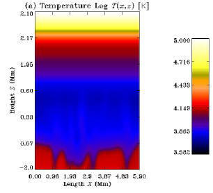
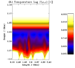
Figure 2: Temperature structure $T$ (in log scale) in the MHD-FALC atmosphere. Panel (b) shows the variation in a smaller range of temperature $T$ between 3819 K and 10000 K.

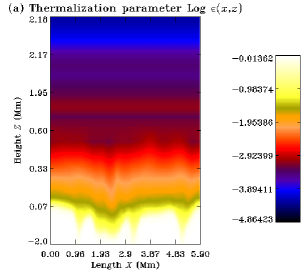
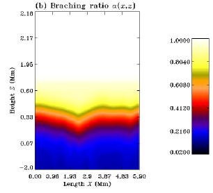
Figure 3: The spatial variation of thermalization parameter $\epsilon$ (in log scale) and the branching ratio $\alpha$ (that appears in the PRD matrices) in the MHD-FALC atmosphere.

In this section we focus our attention on the spatial variation of some of the crucial physical parameters on which the variation of the linearly polarized profiles sensitively depend. In Figures 2(a) and (b) we show the structure of temperature (in log scale) in the MHD-FALC atmosphere along $X$ and $Z$ directions. In Figures 3(a) and (b) we show respectively the thermalization parameter $\epsilon$ (in log scale) and the branching ratio $\alpha=\Gamma_{R}/(\Gamma_{R}+\Gamma_{E}+\Gamma_{I})$ that multiplies $r_{\rm II}$ function in the PRD matrices (Bommier, 1997b). Color bars in the respective figures represent the range of variation of the values of the physical parameters shown in corresponding figures.

In Figure 2(a) we show the temperature structure Log $T$ in the MHD-FALC atmosphere, with $T$ in the range 3819 K to 10⁵ K. Since the variation spans a wide range of values, the image looks nearly the same in the heights between 0.07 Mm to 0.65 Mm. To show the actual temperature variation in these heights we restrict the upper limit of temperature to 10⁴ K in Figure 2(b), where one can notice a significant horizontal and vertical variation of temperature. Above $\sim$ 0.65 Mm there is no horizontal inhomogeneity in the MHD-FALC atmosphere and therefore we see the same temperature in the horizontal direction. The vertical variation in these layers is the same as the well known temperature variation in 1D FALC atmosphere (see e.g., Figure 2 in Anusha et al., 2010).

The spatial variations of $\epsilon$ and $\alpha$ are more interesting for the line formation process. In Figure 3(a) $\epsilon$ approaches unity in the deeper layers which means that the source function has dominant contribution from thermal sources in these layers. A gradual decrease in the value of $\epsilon$ with increase in height shows the increased contribution from scattering sources in those layers. $\epsilon$ shows some horizontal variations in the layers below 0.65 Mm. The parameter $\alpha$ shown in Figure 3(b) multiplies the $r_{\rm II}$ function in the redistribution matrices and it represents the probability of frequency coherent scattering (in the atom’s rest frame) in the medium. It approaches unity in the layers above 0.65 Mm showing that contribution from $r_{\rm II}$ dominates over that from $r_{\rm III}$ in these layers. In between 0.2 Mm to 0.65 Mm, $\alpha$ takes values between 0.3 – 0.9 which means that $r_{\rm II}$ continues to have a significant contribution to the line formation in these layers. In the deepest layers where collisions dominate over scattering, $\alpha$ takes smaller values ($\sim$ 10^-2). In these layers contribution from $r_{\rm III}$ redistribution dominates over $r_{\rm II}$.

5 CONTRIBUTION FUNCTIONS

In this section we discuss the contribution functions in the context of 2D RT and the corresponding heights of formation of the Ca ii K line at different wavelength points.

Following Magain (1986) the contribution function $C_{I}$ for the specific intensity in the context of 2D RT may be defined as

$$C_{I}(\lambda,\bm{r},\bm{\Omega})=\frac{1}{c_{s}(\bm{\Omega})}\ln(10)\frac{\kappa_{\rm tot}(\lambda,\bm{r})}{\kappa_{\rm tot}(\lambda_{0},\bm{r})}$$

$$s(\lambda_{0},\bm{r},\bm{\Omega})S(\lambda,\bm{r})\exp\left[{-s(\lambda,\bm{r},\bm{\Omega})}\right].$$ (18)

Here $S(\lambda,\bm{r})$ is the unpolarized source function and $s(\lambda,\bm{r},\bm{\Omega})$ is the photon path length defined as

$$s(\lambda,\bm{r},\bm{\Omega})=\int_{\textrm{path}}ds(\lambda,\bm{r},\bm{\Omega}),\quad{\textrm{with}}$$

$$ds(\lambda,\bm{r},\bm{\Omega})=\kappa_{\rm tot}(\lambda,\bm{r})d{\rm x}/c_{s}(\bm{\Omega})\quad{\textrm{or}}$$

$$=\kappa_{\rm tot}(\lambda,\bm{r})d{\rm z}/c_{s}(\bm{\Omega}),$$ (19)

where the direction cosine $c_{s}(\bm{\Omega})=\gamma$ if the ray hits the horizontal $X$ axis and $c_{s}(\bm{\Omega})=\mu$ if the ray hits the vertical $Z$ axis when it passes through the 2D medium (see Kunasz & Auer, 1988).

The spatially averaged contribution functions $<C_{I}>$ are obtained by performing an arithmetic averaging of $C_{I}$ over the spatial $X$ grid. In Figure 4 we plot $<C_{I}>$ for 5 selected wavelengths and two ray directions chosen to represent a near-limb and a near-disk-center lines of sight. In Table 1 these 5 selected wavelengths and the height at which $<C_{I}>$ reaches its maximum value are tabulated, which can be considered to be an approximate line formation height at that wavelength.

Table 1: The line formation heights (in Mm) at different wavelengths for near-limb and near-disk-center lines of sight.

$\lambda$	Near-limb	Near-disk-center
3928.15 Å	0.25 Mm	0.2 Mm
3933.09 Å	0.65 Mm	0.5 Mm
3933.50 Å	2.15 Mm	1.27 Mm
3933.65 Å	2.16 Mm	2.16 Mm
3933.80 Å	2.16 Mm	1.17 Mm

For both the directions considered here, the far wings ($\sim$ 3928.15 Å ) and the near wings ($\sim$ 3933.09 Å ) are formed at or below 0.65 Mm. For the near-limb line of sight, the line core region (3933.50 Å –3934 Å ) including blue core minimum ($\sim$ 3933.50 Å ), red core minimum ($\sim$ 3933.80 Å ) and the line center ($\sim$ 3933.65 Å ) are formed higher up in the atmosphere between 2 Mm – 2.5 Mm. For the near-disk-center line of sight line center is formed between 2 Mm to 2.5 Mm, but the core minima are formed just above 1 Mm. The heights of formation are very useful to understand the spatial distribution of the linear polarization discussed in Section 6.

6 RESULTS AND DISCUSSIONS

In this section we discuss the results of our investigations on the nature of the Stokes profiles calculated using our 2D polarized RT code with PRD as the scattering mechanism. The focus is on (1) the spatial variations of the Stokes profiles and (2) comparison of the observed and synthetic Stokes profiles computed from our code.

6.1 Spatial variation of the Stokes profiles

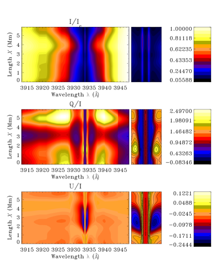
Figure 5: Spatial and spectral variation of $I/I_{c},Q/I,U/I$ for $(\mu,\varphi)=(0.3,160^{\circ})$. The spatial dimension ($X$) represents the horizontal variation on the surface of a 2D atmosphere. The magnetic field configuration is $(B,\theta_{B},\chi_{B})=(20\,{\textrm{G\,}},45^{\circ},225^{\circ})$. The middle panels show the same profiles in a smaller wavelength range between 3932.9 Å  to 3934.2 Å . This simulated image can be visualized as analogous to a spectrum obtained from an imaging spectrograph, with wavelength information on the horizontal axis and spatial information along the slit on the vertical axis.

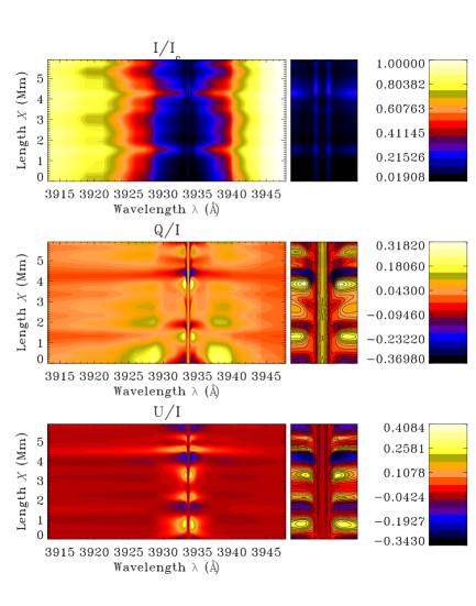
Figure 7: Same as Figure 5, but for $(\mu,\varphi)=(0.8,135^{\circ})$.

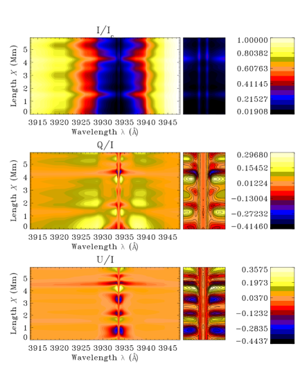
Figure 8: Same as Figure 6 but for $(\mu,\varphi)=(0.8,225^{\circ})$.

It is well known that the strong resonance lines with broad wings have their origin in the PRD coherent scattering mechanism ($r_{\rm II}$ redistribution). When combined with multi-D RT, the PRD effects manifest themselves also through enhanced inhomogeneous spatial distribution of the linear polarization profiles in the line wings (see e.g., Anusha & Nagendra, 2011b). In that paper we consider an isothermal atmosphere. Temperature structure of the realistic atmosphere further enhances the inhomogeneities. These characteristics can be clearly seen in Figures 5–8 which we discuss below.

In Figures 5–8 we show the spatial variations of the emergent synthetic spectra of Ca ii K line at 3933 Å  computed using MHD-FALC atmosphere. We present the images of the $(I/I_{c},Q/I,U/I)$ with the $\lambda$-scale on the abscissae (covering the range 3913 Å –3948 Å ) and the $X$-scale on the ordinates. The images cover a range of values between minima and maxima of the Stokes profiles. We have considered four directions namely $(\mu,\varphi)$=$(0.3,160^{\circ})$, $(0.3,200^{\circ})$, $(0.8,135^{\circ})$ and $(0.8,225^{\circ})$. The two chosen $\mu$ values represent near-limb ($\mu=0.3$) and near-disk-center ($\mu=0.8$) lines of sight. We chose two magnetic field ($\bm{B}$) configurations given by $(B,\theta_{B},\chi_{B})$ $=(20\,{\textrm{G}\,},45^{\circ},225^{\circ})$ and $(20\,{\textrm{G}\,},75^{\circ},225^{\circ})$. We assume the magnetic field $\bm{B}$ to be independent of spatial co-ordinates $X$ and $Z$. For clarity, the line core region is magnified in the middle panels in Figures 5–8. The wavelength range in these panels is 3932.9 Å  to 3934.2 Å . For the sake of discussions we refer to the spectrum in the wavelength range 3933.5 Å–3934 Å  as the line core and those in the range 3913 Å–3933.5 Å  and 3934 Å –3948 Å  as the line wings.

6.1.1 General characteristics

First we remark that due to the periodicity of the medium in the horizontal direction considered for the calculations, the spatial distribution of $I/I_{c}$, $Q/I$ and $U/I$ is also periodic with respect to the horizontal $X$ direction. As discussed in Section 5 and Table 1 the Ca ii K line wings are formed at or below a height of $\sim$ 0.65 Mm, and the line core is formed above this height. We note that 0.65 Mm is the approximate height at which the MHD-FALC atmosphere changes from 2D-MHD variation to horizontally homogeneous stratification represented by the 1D FALC atmosphere. Therefore, the spatial structuring in the lower atmosphere causes significant spatial inhomogenity in the wings of $(I/I_{c},Q/I,U/I)$ and spatial homogeneity (in the horizontal direction) in the higher layers of the atmosphere causes spatial homogeneity in the line core. This is true for all the lines of sight in Figures 5– 8.

6.1.2 Intensity distribution

A comparison of the spatial distribution of $I/I_{c}$ in Figures 5–8 show that the emergent intensity is not as sensitive to the radiation azimuth $(\varphi)$ as it is to the co-latitude $\theta$. In other words the center to limb variation of $I/I_{c}$ is stronger than the axial-asymmetry of the emergent radiation field. In the far wings $I/I_{c}$ approaches unity, clearly because it is normalized to the nearby continuum value.

6.1.3 $Q/I$ and $U/I$ in the line wings

Spatial distribution of $Q/I$ and $U/I$ for near-limb and near-disk-center lines of sight have considerable differences (compare Figure 5 with 7 and 6 with 8). For example, in Figures 5 and 7, $|Q/I|_{\rm max}$ amplitudes decrease from 2.5 % to 0.36 % from near-limb to the near-disk-center, and $|U/I|_{\rm max}$ amplitudes increase from 0.24 % to 0.40 %. The distribution appears in the form of several domains within which $Q/I$ and $U/I$ values are slowly varying.

The $Q/I$ and $U/I$ distributions in the wings respectively show a symmetry and antisymmetry with respect to the radiation azimuth belonging to two opposing octants about the symmetry axis, for a given value of $\mu$ (compare Figure 5 with 6 and 7 with 8). This is a behavior of the Rayleigh scattered polarized radiation field in a 2D medium with respect to the symmetry axis (see Appendix B of Anusha et al., 2011a, for a proof). Since Hanle scattering affects only the line core, and the Rayleigh scattering limit is recovered in the wings, we see the symmetries discussed above, only in the wings of these images. We note here that the azimuths in Figures 5 and 7 lie on one side of the symmetry axis ($160^{\circ}$ and $135^{\circ}$ respectively) and those in Figures 6 and 8 lie on the other side ($200^{\circ}$ and $225^{\circ}$ respectively) because of which symmetry relations become valid. Exact symmetry anti-symmetry in the values of $Q/I$ and $U/I$ can be seen if the azimuths differ exactly by 180^∘. However we do not show them here, as those azimuths do not fall on the Carlsson grid points.

An important difference between 1D and multi-D RT is that, in the case of resonance scattering, multi-D geometry produces a non-zero $U/I$ throughout the line profile, but the 1D geometry does not produce any $U/I$. The Hanle scattering produces non-zero $U/I$ in 1D geometry only in the line core, where as in multi-D RT Hanle scattering only modifies the $U/I$ generated by the resonance scattering. Further, a strong $\lambda$ dependence of the spatial distribution shows that the scattering physics described through PRD strongly couples with spatial inhomogenity of the atmosphere.

Spatial variations in the linear polarization profiles are observationally noticed in the wings of the well known chromospheric line, the Ca i 4227 Å  (see Bianda et al., 2003; Sampoorna et al., 2009), which the authors refer to as the ‘enigmatic wing features’. We find such spatial inhomogeneities in the line wings of Ca ii K line, which is also a chromospheric line. Therefore we believe through our studies that, the spatial variations observed in the wings of chromospheric lines possibly have their origin in the spatial structuring of the atmosphere. To understand and model these observations, accurate non-LTE multi-D RT calculations with PRD scattering are essential. We note here that even in an isothermal atmosphere the multi-D RT can cause strong spatial inhomogeneities in the line wings through spatial structuring (namely the geometry itself, see Figures 13 and 14 of Anusha & Nagendra, 2011b). As it is well known, the approximation of CRD cannot explain such spatial structuring, because $Q/I$ and $U/I$ approach zero in the line wings, under this approximation.

6.1.4 $Q/I$ and $U/I$ in the line core

It may be interesting to notice that the linear polarization observations of the Ca ii K line at 3933 Å  in the line core region studied in Stenflo (2006) show a strong spatial variation (in the range 3933.5 Å –3934 Å ). Such spatial variations are caused by (1) spatially varying magnetic fields (Hanle effect) and (2) spatial inhomogeneities of the atmosphere itself. These two factors are entangled with each other in the line core and are hard to be separated. Since the atmosphere chosen in this paper does not have any horizontal inhomogeneity in the heights where the line core is formed, we discuss only the magnetic field effects (Hanle effect) on the line core in this paper (see Figures 5–8, particularly the middle panels).

In our studies we consider two different, spatially independent (i.e., constant) magnetic field configurations (see Section 6.1). Changes in the values of $Q/I$ and $U/I$ in the line core for two magnetic field values can be clearly observed by comparing middle panels of Figures 5 and 7 with the corresponding panels of Figures 6 and 8 respectively. Also one can observe faint spatial variation in the line core in each of these figures. Spatial homogeneity in the large parts of the line core is due to the homogeneity of the chosen model atmosphere in the heights where the line core is formed and also because of the spatially independent magnetic field configurations. Considering a magnetic field configuration that depends explicitly on spatial variables $(x,z)$ and perhaps also on the angular variables $(\theta,\varphi)$ and/or the use of atmosphere with spatial inhomogeneity in the chromosphere may result in a spatially varying line core polarization similar to those in Stenflo (2006). However we do not take up such studies in this paper.

Here one can observe that the symmetry, anti-symmetry of $Q/I$ and $U/I$ in the line wings (see Section 6.1.3) breaks in the line core region due to the presence of magnetic fields (see Anusha et al., 2011a, for details).

6.2 Comparisons with observations

In Holzreuter et al. (2006); Holzreuter & Stenflo (2007a) and Holzreuter & Stenflo (2007b) the authors study in detail, the linear polarization ($Q/I$) in Ca ii K line at 3933 Å  using 1D solar model atmospheres. Their studies suggest that ‘none of the existing 1D model atmospheres are able to reproduce the observations at different $\mu$ values’. They find that by modifying the temperature structure one could find optimum fits to the observations. However a single model atmosphere with a fixed temperature structure could not fit the observed $Q/I$ at different $\mu$ values. In other words observations of $Q/I$ at different $\mu$ values required different modifications of the temperature structure of the chosen 1D model atmosphere such as FALC (see Holzreuter & Stenflo, 2007a). They conclude that use of multi-D MHD atmospheres with multi-D RT may be necessary to fit the observations at different $\mu$ values using a single model atmosphere.

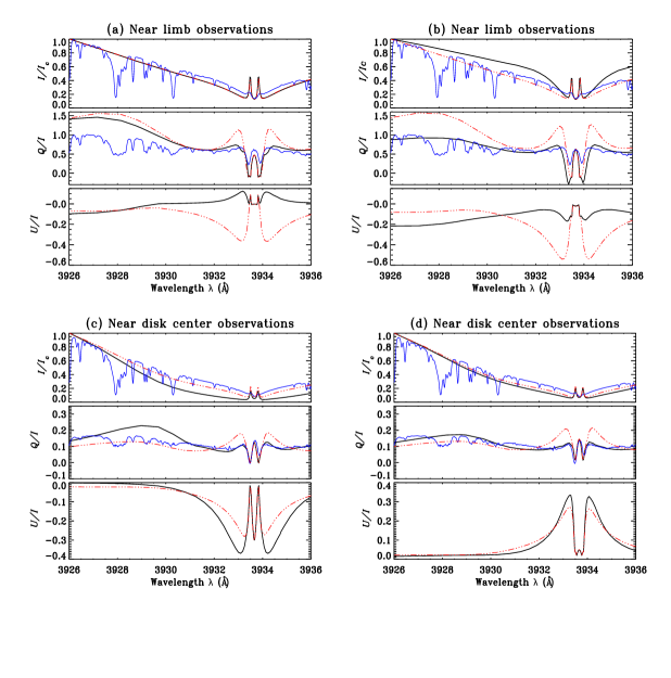
Figure 9: Comparison of $(I/I_{c},Q/I)$ observations of the Ca ii K line with the theoretical $(I/I_{c},Q/I,U/I)$ profiles. We show observations (blue solid lines), spatially averaged theoretical profiles (red dash-triple-dotted lines) and spatially resolved theoretical profiles (black solid lines). The ray directions, spatial locations (for spatially resolved curves only) and the magnetic field configurations considered in panels (a)–(d) are respectively: (a): $(\mu,\varphi)=(0.3,111^{\circ})$, $X=$0.45 Mm, $\bm{B}=(20\,{\rm G\,},90^{\circ},225^{\circ})$, (b): $(\mu,\varphi)=(0.3,70^{\circ})$, $X=$0.51 Mm, $\bm{B}=(13\,{\rm G\,},90^{\circ},225^{\circ})$ (c): $(\mu,\varphi)=(0.8,45^{\circ})$, $X=$0.1 Mm, $\bm{B}=(20\,{\rm G\,},45^{\circ},45^{\circ})$ and (d): $(\mu,\varphi)=(0.8,315^{\circ})$, $X=$0.54 Mm, $\bm{B}=(60\,{\rm G\,},120^{\circ},45^{\circ})$.

In this paper we do not attempt to model the observed profiles through modifications of the temperature structure in the atmosphere. Our aim is to study how well the structuring in the model atmosphere can reproduce the observed $(I/I_{c},Q/I)$ profiles. In addition to the spatially averaged, emergent ($Z=Z_{\rm max}$) $(I/I_{c},Q/I)$ profiles (averaged over the $X$ grid) we compare the observed profiles with the emergent $(I/I_{c},Q/I)$ profiles at each of the 62 grid points along the $X$ direction and try to fit the observations. We consider such comparisons because in general, spatial averaging is reasonable if the profiles do not show strong spatial variations. However the linear polarization that we have obtained from the MHD-FALC atmosphere is extremely spatially inhomogeneous in the line wings (see Figures 5–8). Since each of these 62 points correspond to a different spatial location, the profiles at these points are also different. In Figure 9 we plot observed $(I/I_{c},Q/I)$ profiles (blue solid lines) with spatially averaged, emergent $(I/I_{c},Q/I,U/I)$ profiles (red dash-triple-dotted lines) and spatially resolved $(I/I_{c},Q/I,U/I)$ profiles (black solid lines).

6.2.1 The line wings

The MHD-FALC atmosphere chosen in this paper has spatial inhomogeneities only up to a height of $\sim$ 0.65 Mm. Since the line wings (defined in Section 6.1) are formed at or below this height (see Section 5 and Table 1), we expect that the line wings should be well reproduced by the MHD-FALC atmosphere. In Figure 9 we can see that better fit to the envelop of the wings of the $I/I_{c}$ profiles could be obtained with the spatially averaged profiles than with the spatially resolved ones. However for the $Q/I$, the spatially averaged profiles could not fit the observations at all, perhaps because the wing polarization is extremely spatially inhomogeneous. We could reasonably fit the line wings only by using the spatially resolved profiles. In Figure 9 (a)–(d) the profiles are plotted for the spatial locations $X=$ 0.45 Mm, 0.51 Mm, 0.1 Mm and 0.54 Mm respectively. In the case of near-limb observations, we could not obtain a simultaneous fit to the far and the near wings at any of the 62 spatial locations. Figure 9(a) is an example of a reasonable fit to the near wings and Figure 9(b) for the far wings. Since the far wings are formed well below 0.65 Mm, we expect the MHD variation in this lower atmosphere to well reproduce them. The near wings are difficult to reproduce using MHD-FALC atmosphere because, the near wing region which we are unable to fit in Figure 9(b) is formed just around the height $\sim 0.65$ Mm (see Figure 4(a)) which is the height at which the atmosphere changes from 2D-MHD variation to 1D FALC, and thus around these heights, the atmosphere may have some deficiencies. In the case of near-disk-center observations, Figure 9(d) represents a better fit to the line wings (both near and far) than Figure 9(c). We are able to reasonably fit the near-wings in this case because they are formed around $\sim 0.5$ Mm (see Figure 4(b)) where the atmosphere is well represented by MHD variations.

6.2.2 The line core

The line core is formed above a height of 0.65 Mm (see Section 5) where the MHD-FALC atmosphere does not have any horizontal inhomogeneities. Therefore we do not expect the atmosphere to provide a good fit to the observations. We see that in Figure 9 even the $I/I_{c}$ profiles are not well fitted. However by computing the theoretical profiles for several magnetic field configurations, it is possible to obtain a good fit to the line center value of $Q/I$. The optimum values of the magnetic fields for obtaining the fit in Figure 9 are: $\bm{B}=(20\,{\rm G\,},90^{\circ},225^{\circ})$ for panel (a), $\bm{B}=(13\,{\rm G\,},90^{\circ},225^{\circ})$ for panel (b), $\bm{B}=(20\,{\rm G\,},45^{\circ},45^{\circ})$ for panel (c) and $\bm{B}=(60\,{\rm G\,},120^{\circ},45^{\circ})$ for panel (d). The choice of different magnetic fields helped to obtain a reasonable fit to the line core $Q/I$ in the case of near-disk-center observations. We could not reproduce the line core of $Q/I$ (except the line center) for near-limb observations for any choice of the magnetic field values that we considered. The fact that 1D models can reproduce the observations of the line core of the near-disk-center but not those of the near-limb is also true for the Ca i 4227 Å  line, which we found in our previous studies (see Anusha et al., 2010, 2011b). This would perhaps indicate that the heights at which line cores are formed in the case of near-limb observations are more inhomogeneous than the heights where the line core is formed in the case of the near-disk-center observations (see Section 5, Figure 4 and Table 1). However, we cannot attribute it to the goodness of the atmosphere because a consistent atmosphere will have inhomogeneities at all the heights and it should be able to reproduce the entire line profile at all the lines of sight.

7 CONCLUSIONS

This paper represents the first application of our work in a previous series of papers on polarized RT in multi-D media. Here we develop the necessary code, test it and use it to study the linear polarization in the Ca ii K line at 3933 Å . This work is an initial step towards modeling the chromospheric lines because here we choose an approximate model atmosphere. It is a 2D snapshot of an MHD atmosphere in the photosphere combined with columns of 1D FALC atmosphere in the chromosphere. The use of PRD as the line scattering mechanism is essential in the modeling effort, because the approximation of CRD leads to nearly zero linear polarization in the line wings.

The MHD structuring in the photosphere produces spatial inhomogeneities in the wings of the linear polarization profiles and it explains the causes of spatial structuring observed in the wings of some strong chromospheric lines.

Since the atmosphere that we have used can represent the MHD structuring up to a height of $0.65$ Mm, the wavelength region of the $Q/I$ profiles formed below this height could be fitted reasonably well. This includes far wings for both the lines of sight (near limb and near-disk-center), near wings in the case of near-disk-center observations. Using different magnetic field configurations and Hanle effect we obtained reasonable fits to the line center values of $Q/I$ for both the lines of sight. In the case of near-limb observations, the near wings and the line core region including core minima could not be fitted using this atmosphere. Although we could fit the line core region in the case of near-disk-center observations, the reason for a good fit cannot attributed to the goodness of the atmosphere because the same atmosphere could not produce the line core in the case of near-limb observations.

This study clearly indicates that as in the photosphere, MHD structuring in the chromosphere is an important requirement to obtain simultaneous fit to the line core and the line wing polarization observations of the chromospheric lines at all the lines of sight. To achieve this, we need 3D MHD model atmospheres that can quite well represent the solar chromospheric inhomogeneities.

Appendix A Pre-BiCG-STAB algorithm

In this Appendix we describe some important steps in the Pre-BiCG-STAB algorithm, to be taken care when using the method to model spectral lines, for which both line and continuum scattering processes become important.

Using the formal solution expression for $\bm{\mathcal{I}}$, the vector $\bm{\mathcal{J}}$ in Equation (14) can be written as

$$\bm{\mathcal{J}}(\lambda,\bm{r})=\Lambda[\bm{\mathcal{S}}(\lambda,\bm{r})].$$ (A1)

Similarly the continuum source vector in Equation (15) can be written as

$${\bm{\mathcal{S}}}_{c}(\lambda,\bm{r})=\Lambda_{c}[\bm{\mathcal{S}}(\lambda,\bm{r})].$$ (A2)

Recall the total source vector expression given by

$$\bm{\mathcal{S}}(\bm{r},x)=p_{l}[\epsilon{B}_{\lambda}(\bm{r})\bm{\mathcal{U}}+\bm{\mathcal{J}}(\bm{r},x)]+p_{c}\bm{\mathcal{S}}_{c}(\lambda,\bm{r})+p_{a}{B}_{\lambda}(\bm{r})\bm{\mathcal{U}}.$$ (A3)

Substituting Equations (A1) and (A2) in Equation (A3), we obtain a system of equations

$$\hat{A}\bm{\mathcal{S}}=\bm{b}\quad\quad\textrm{or}\quad\quad[\hat{I}-p_{l}\Lambda-p_{c}\Lambda_{c}]\bm{\mathcal{S}}(\lambda,\bm{r})=[p_{l}\epsilon+p_{a}]{B}_{\lambda}(\bm{r})\bm{\mathcal{U}}.$$ (A4)

Let $\bm{\mathcal{S}}_{0}$ denote an initial guess for the source vector. In this paper we calculate the initial source vector using the unpolarized mean intensity obtained by solving the unpolarized multi-level RT equation in the RH-code. The rest of the algorithm is similar to that described in Anusha et al. (2011a).

Figure 1: This figure shows the geometry of the atmosphere that we have used, namely a 2D cross section of a 3D MHD atmosphere in the photosphere and columns of FALC atmosphere in the chromosphere. The emergent solutions on the line $(X,Z_{\rm max})$ marked here, are shown as images in the Figures 5-8.

Figure 4: Spatially averaged contribution function at selected wavelengths. Panel (a) is for near-limb direction $(\mu,\varphi)=(0.3,160^{\circ})$ and panel (b) for a near-disk-center direction $(\mu,\varphi)=(0.8,135^{\circ})$. We have normalized the $<C_{I}>$ by the maximum value of $<C_{I}>$.

Figure 6: Same as Figure 5, but for $(\mu,\varphi)=(0.3,200^{\circ})$ and magnetic field configuration $(B,\theta_{B},\chi_{B})=(20\,{\textrm{G\,}},75^{\circ},225^{\circ})$.

References

- Anusha & Nagendra (2011a) Anusha, L. S., & Nagendra, K. N. 2011a, ApJ, 726, 6
- Anusha & Nagendra (2011b) Anusha, L. S., & Nagendra, K. N. 2011b, ApJ, 738, 116
- Anusha & Nagendra (2011c) Anusha, L. S., & Nagendra, K. N. 2011c, ApJ, 739, 40
- Anusha & Nagendra (2011d) Anusha, L. S., & Nagendra, K. N. 2011d, ApJ, 746, 84
- Anusha et al. (2009) Anusha, L. S., Nagendra, K. N., Paletou, F., & Léger, L. 2009, ApJ, 704, 661
- Anusha et al. (2010) Anusha, L. S., Nagendra, K. N., Stenflo, J. O., Bianda, M., Sampoorna, M., Frisch, H., Holzreuter, R., & Ramelli, R. 2010, ApJ, 718, 988
- Anusha et al. (2011a) Anusha, L. S., Nagendra, K. N., & Paletou, F. ApJ, 2011a, 726, 96
- Anusha et al. (2011b) Anusha, L. S., Nagendra, K. N., Bianda, M., Stenflo, J. O., Holzreuter, R., Sampoorna, M., Frisch, H., Ramelli, R. & Smitha, H. N., 2011b, ApJ, 737, 95
- Auer & Paletou (1994) Auer, L. H., & Paletou, F. 1994, A&A, 285, 675
- Bianda et al. (2003) Bianda, M., Stenflo, J. O., Gandorfer, A., & Gisler, D. 2003, in ASP Conf. Ser. 286, Current Theoretical Models and Future High Resolution Solar Observations: Preparing for ATST, ed. A. A. Pevtsov & H. Uitenbroek (San Francisco: ASP), 61
- Bommier (1997a) Bommier, V. 1997a, A&A, 328, 706
- Bommier (1997b) Bommier, V. 1997b, A&A, 328, 726
- Chandrasekhar (1960) Chandrasekhar, S. 1960, Radiative Transfer (New York: Dover)
- Carlsson (2009) Carlsson, M. 2009, Mem.S.A.It, 80, 606
- Faurobert-Scholl (1992) Faurobert-Scholl, M. 1992, A&A, 258, 521
- Fontenla et al. (1993) Fontenla, J. M., Avrett, E. H., & Loeser, R. 1993, ApJ, 406, 319
- Frisch (2007) Frisch, H. 2007, A&A, 476, 665
- Frisch et al. (2012) Frisch, H., Anusha, L. S., Bianda, M., Holzreuter, R., Nagendra, K. N., Ramelli, R., Sampoorna, M., Smitha, H. N., & Stenflo, J. O., 2012, in EAS Publications Series 55, 59
- Gandorfer et al. (2004) Gandorfer, A. M., Povel H. P., Steiner, P., Aebersold, F., Egger, U., Feller, A., Gisler, A., Hagenbuch, S., & Stenflo, J. O. 2004, A&A, 422, 703
- Holzreuter et al. (2005) Holzreuter, R., Fluri, D. M., & Stenflo, J. O. 2005, A&A, 434, 713
- Holzreuter et al. (2006) Holzreuter, R., Fluri, D. M., & Stenflo, J. O. 2006, A&A, 449, L41
- Holzreuter & Stenflo (2007a) Holzreuter, R., & Stenflo, J. O. 2007a, A&A, 467, 695
- Holzreuter & Stenflo (2007b) Holzreuter, R., & Stenflo, J. O. 2007b, A&A, 472, 919
- Hummer (1962) Hummer, D. G. 1962, MNRAS, 125, 21
- Kunasz & Auer (1988) Kunasz, P., & Auer, L. H. 1988, JQSRT, 39, 67
- Landi Degl’Innocenti & Landolfi (2004) Landi Degl’Innocenti, E., & Landolfi, M. 2004, Polarization in Spectral Lines (Dordrecht: Kluwer)
- Magain (1986) Magain, P. 1986, A&A, 163, 135
- Nordlund & Stein (1991) Nordlund, Å ., & Stein, R. F., 1991, in Stellar Atmospheres: Beyond Classical Models, NATO ASI Series C, 341, ed. L. Crivellari, I. Hubeny, & D. G. Hummer (Dordrecht: Kluwer), 263
- Rybicki & Hummer (1991) Rybicki, G. B., & Hummer, D. G. 1991, A&A, 245, 171
- Rybicki & Hummer (1992) Rybicki, G. B., & Hummer, D. G. 1992, A&A, 262, 209
- Sampoorna et al. (2009) Sampoorna, M., Stenflo, J. O., Nagendra, K. N., Bianda, M., Ramelli, R., & Anusha, L. S. 2009, ApJ, 699, 1650
- Shchukina & Trujillo Bueno (2007) Shchukina, N.,& Trujillo Bueno, J. 2011, ApJ, 731, L21
- Stenflo (2006) Stenflo, J. O. 2006, in ASP Conf. Ser. 358, Solar Polarization 4, eds. R. Casini, & B. W. Lites (San Francisco: ASP), 215
- Trujillo Bueno & Shchukina (2007) Trujillo Bueno, J, & Shchukina, N. 2007, ApJ, 664, 135
- Trujillo Bueno et al. (2004) Trujillo Bueno, J., Shchukina, N., & Asensio Ramos, A. 2004, Natur. 430, 326
- Uitenbroek (2000) Uitenbroek, H. 2000, ApJ, 531, 571
- Uitenbroek (2001) Uitenbroek, H. 2001, ApJ, 557, 389
- Uitenbroek (2006) Uitenbroek, H. 2006, ApJ, 639, 516
- Vögler et al. (2005) Vögler, A., Shelyag, S., Schüssler, M., Cattaneo, F., Emonet, T., & Linde, T. 2005, A&A, 429, 335