DESY-13-143

TUM-HEP 901/13

FLAVOUR-EU 52/13

A note on discrete $\boldsymbol{R}$ symmetries
in $\boldsymbol{\mathbbm{Z}_{6}}$–II orbifolds with Wilson lines

Hans Peter Nilles^a, Saúl Ramos–Sánchez^b, Michael Ratz^c, Patrick K.S. Vaudrevange^d

^a Bethe Center for Theoretical Physics
and
Physikalisches Institut der Universität Bonn,
Nussallee 12, 53115 Bonn, Germany

^b Department of Theoretical Physics, Physics Institute, UNAM
  Mexico D.F. 04510, Mexico

^c Physik-Department T30, Technische Universität München,
  James-Franck-Straße, 85748 Garching, Germany

^d Deutsches Elektronen-Synchrotron DESY,
  Notkestraße 85, 22607 Hamburg, Germany

We re–derive the $R$ symmetries for the $\mathbbm{Z}_{6}$–II orbifold with non–trivial Wilson lines and find expressions for the $R$ charges which differ from those in the literature.

1 Introduction

$R$ symmetries play a key role in understanding supersymmetric field theories and in model building. It is well known that $R$ symmetries do arise from the Lorentz symmetry of compact dimensions. In many cases the compact dimensions only have discrete isometries, leading to discrete $R$ symmetries in the effective four–dimensional (4D) theory. This is, in particular, true for orbifold compactifications [1, 2].

In the past, $R$ symmetries have been derived for the case of $\mathbbm{Z}_{6}$–II orbifold compactifications of the heterotic string [3]. Later it was observed in [4] that, unlike all other continuous and discrete symmetries of the effective 4D description of these settings, the $\mathbbm{Z}_{M}^{R}$ symmetries have non–universal anomalies. This already suggested that there might be something wrong with the $R$ charges. And, indeed, more recently it was pointed out in [5] that the $R$ charges have to be amended by contributions from so–called $\gamma$ phases. The purpose of this note is to re–derive the $R$ symmetries and charges for the $\mathbbm{Z}_{6}$–II orbifold, and to clarify the situation. Moreover, our re–derivation allows us to determine the $R$ charges also in settings with non–trivial Wilson lines.

This note is organized as follows. Section 2 contains our re–derivation of $R$ symmetries and charges. Finally, section 3 contains our conclusions, including a brief discussion of the implications of the correct charges for model building.

2 Discrete $\boldsymbol{R}$ symmetries in $\boldsymbol{\mathbbm{Z}_{6}}$–II orbifolds

After a brief introduction to the $\mathbbm{Z}_{6}$–II orbifold in section 2.1 we discuss the origin of discrete $R$ symmetries in section 2.2. In section 2.3 we derive previously unknown contributions to the $R$ charges, which turn out to be essential in order to make the corresponding discrete anomalies universal, such that they can be cancelled by the dilaton via the Green–Schwarz mechanism.

2.1 The $\boldsymbol{\mathbbm{Z}_{6}}$–II orbifold

The $\mathbbm{Z}_{6}$–II orbifold is defined as the quotient space of the six–dimensional torus $\mathbbm{T}^{6}$ by the point group $P=\mathbbm{Z}_{6}$,

$$\mathbbm{O}~{}=~{}\mathbbm{T}^{6}/P~{}=~{}\mathbbm{C}^{3}/\mathbbm{S}\;.$$ (1)

The generator of $\mathbbm{Z}_{6}$ is denoted as $\theta$ with $\theta^{6}=\mathbbm{1}$. For $\mathbbm{Z}_{6}$–II it is represented by the so–called twist vector

$$v~{}=~{}\left(0,\frac{1}{6},\frac{1}{3},-\frac{1}{2}\right)\;,$$ (2)

which specifies the rotational angles as fractions of $2\pi$ in the three complex planes, i.e. the three complex torus–coordinates $z^{i}$ get mapped to $\mathrm{e}^{2\pi\,\mathrm{i}\,v^{i}}\,z^{i}$ for $i=1,2,3$ and $v^{0}=0$ for later convenience. The twist acts on the factorized six–torus $\mathbbm{T}^{6}=\mathbbm{T}_{\mathrm{G}_{2}}^{2}\times\mathbbm{T}_{\mathrm{SU}(3)}^{2}\times\mathbbm{T}^{2}_{\mathrm{SU}(2)\times\mathrm{SU}(2)}$ (see figure 1), whose defining six–dimensional lattice $\Lambda$ is given by the root lattice of $\text{G}_{2}\times\mathrm{SU}(3)\times\mathrm{SU}(2)^{2}$.

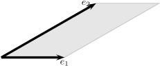
(a) $\mathbbm{T}_{\mathrm{G}_{2}}^{2}$.

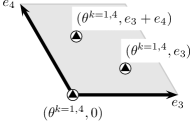
(b) $\mathbbm{T}_{\mathrm{SU}(3)}^{2}$.

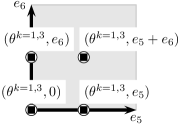
(c) $\mathbbm{T}_{\mathrm{SU}(2)\times\mathrm{SU}(2)}^{2}$.

Figure 1: The factorized lattice $\Lambda$ of the six–torus is chosen to be spanned by the roots of $\text{G}_{2}\times\mathrm{SU}(3)\times\mathrm{SU}(2)^{2}$. The six vectors $e_{\alpha}$ denote a basis. For later convenience, we show also the fixed points in the $\mathrm{SU}(3)$ and $\mathrm{SU}(2)\times\mathrm{SU}(2)$ planes.

Equivalently, one can define the orbifold $\mathbbm{O}$ as the quotient space of $\mathbbm{C}^{3}$ by the so–called space group $\mathbbm{S}$, see equation (1). Elements of $\mathbbm{S}$ are of the form $g=\left(\theta^{k},n_{\alpha}\,e_{\alpha}\right)$ with summation over $\alpha=1,\ldots,6$, $k=0,\ldots,5$, $n_{\alpha}\in\mathbbm{Z}$ and $e_{\alpha}$ denote six basis vectors of the torus–lattice $\Lambda$. $g$ acts on $z\in\mathbbm{C}^{3}$ as $z\mapsto g\,z~{}=~{}\theta^{k}\,z+n_{\alpha}\,e_{\alpha}$ and the equivalence relation

$$z~{}\sim~{}g\,z\quad\text{for}\quad g\in\mathbbm{S}\quad\text{and}\quad z\in\mathbbm{C}^{3}$$ (3)

defines the orbifold. For a consistent compactification of the heterotic string on $\mathbbm{O}$ one has to embed the action of $g\in\mathbbm{S}$ into the 16 gauge degrees of freedom of $\mathrm{E}_{8}\times\mathrm{E}_{8}$ or $\mathrm{SO}(32)$, which we denote by $X^{I}$ with $I=1,\ldots,16$: the twist $\theta$ acts as a shift $V^{I}$ and lattice translations by $e_{\alpha}$ are accompanied by Wilson lines $W_{\alpha}^{I}$, both restricted by modular invariance. $g$ acts simultaneously on $z$ and $X$ as

$$z~{}\xmapsto{g}~{}\theta^{k}\,z+n_{\alpha}\,e_{\alpha}\quad\text{and}\quad X~{}\xmapsto{g}~{}X+\pi\,\left(k\,V+n_{\alpha}\,W_{\alpha}\right)\;.$$ (4)

As usual, one associates to $g=\left(\theta^{k},n_{\alpha}\,e_{\alpha}\right)$ the local twist $v_{g}=k\,v$ and the local shift $V_{g}=k\,V+n_{\alpha}\,W_{\alpha}$.

Consider a massless, closed (twisted) string with boundary condition given by $g=\left(\theta^{k},n_{\alpha}\,e_{\alpha}\right)\in\mathbbm{S}$, i.e. $\boldsymbol{Z}(\tau,\sigma+\pi)=g\,\boldsymbol{Z}(\tau,\sigma)$ for the three complex world–sheet bosons $\boldsymbol{Z}$ on $\mathbbm{O}$. After canonical quantization this string can be described schematically by a state of the form

$$\Ket{p_{\mathrm{sh}},q_{\mathrm{sh}},\widetilde{N},\widetilde{N}^{*},g}~{}=~{}\Ket{q_{\text{sh}}}_{\text{R}}\otimes\left(\widetilde{\alpha}^{i}_{-\omega_{i}}\right)^{\widetilde{N}^{i}}\,\left(\widetilde{\alpha}^{\bar{\imath}}_{-1+\omega_{i}}\right)^{\widetilde{N}^{*i}}\Ket{p_{\text{sh}}}_{\text{L}}\otimes\Ket{g}\;,$$ (5)

where R and L denote the right– and left–movers with shifted momenta $q_{\text{sh}}$ and $p_{\text{sh}}$, respectively. Here $q_{\text{sh}}=q+v_{g}$ with $q$ from either the vectorial or spinorial weight lattice of $\mathrm{SO}(8)$, and $p_{\text{sh}}=p+V_{g}$ with $p$ from the $\mathrm{E}_{8}\times\mathrm{E}_{8}$ weight lattice. We use the convention that the number of $-\nicefrac{{1}}{{2}}$ in the spinorial weight lattice is even. Then, $q_{\text{sh}}(\text{boson})=q_{\text{sh}}(\text{fermion})+(\nicefrac{{1}}{{2}},-\nicefrac{{1}}{{2}},-\nicefrac{{1}}{{2}},-\nicefrac{{1}}{{2}})$. As usual, fermions with $q_{\text{sh}}^{0}=-\nicefrac{{1}}{{2}}$ are left–chiral. Further, $\Ket{g}$ specifies the localization of the string as follows. If $k\neq 0$, a string twisted by $g=\left(\theta^{k},n_{\alpha}\,e_{\alpha}\right)$ is localized at some fixed point or fixed torus $f_{g}\in\mathbbm{C}^{3}$, i.e.  $g\,f_{g}=f_{g}$ with $f_{g}$ being the coordinates of the fixed point or fixed torus. We will refer to $g$ as “constructing element” for the corresponding massless mode. Furthermore, the left–moving ground state $\Ket{p_{\text{sh}}}_{\text{L}}$ can be excited by oscillators: in each (complex) direction $i=1,2,3$ and $\bar{\imath}=\bar{1},\bar{2},\bar{3}$ there are $\widetilde{N}^{i}$ excitations with $\widetilde{\alpha}^{i}_{-\omega_{i}}$ and $\widetilde{N}^{*i}$ excitations with $\widetilde{\alpha}^{\bar{\imath}}_{-1+\omega_{i}}$. In the $-1$ ghost picture, this state is created by the vertex operator

$$\boldsymbol{V}^{(g)}_{\!\!-1}~{}=~{}\mathrm{e}^{-\boldsymbol{\phi}}\,\mathrm{e}^{2\mathrm{i}\,q_{\mathrm{sh}}\cdot\boldsymbol{H}}\,\mathrm{e}^{2\mathrm{i}\,p_{\mathrm{sh}}\cdot\boldsymbol{X}}\,\prod_{i=1}^{3}\left(\partial\boldsymbol{Z}^{i}\right)^{\widetilde{N}^{i}}\,\left(\partial\boldsymbol{Z}^{*\,i}\right)^{\widetilde{N}^{*i}}\,\boldsymbol{\sigma}_{g}\;.$$ (6)

In particular, the state $\Ket{g}$ is created by the twist field $\boldsymbol{\sigma}_{g}$.

Selection rules are derived from correlators of vertex operators [6, 7],

$$\mathcal{A}~{}=~{}\left\langle\boldsymbol{V}^{(g_{1})}_{\!\!-1/2}\,\boldsymbol{V}^{(g_{2})}_{\!\!-1/2}\,\boldsymbol{V}^{(g_{3})}_{\!\!-1}\,\boldsymbol{V}^{(g_{4})}_{\!\!0}\ldots\boldsymbol{V}^{(g_{L})}_{\!\!0}\right\rangle\;.$$ (7)

The correlation function (7) factorizes into correlators involving separately the fields $\boldsymbol{\phi}$, $\boldsymbol{X}^{I}$, $\boldsymbol{\sigma_{g}}$, $\boldsymbol{H}$ and $\boldsymbol{Z}^{i}$ [6, 7, 8, 9, 10]. This leads to the condition of gauge invariance, the so–called space group selection rules and to discrete $R$ symmetries as we explain in what follows.

2.2 Discrete $\boldsymbol{R}$ symmetries and sublattice rotations

Discrete $R$ symmetries are intimately connected with so–called sublattice rotations. Since $\mathbbm{O}$ is factorized, $\mathbbm{O}$ respects symmetries beyond the elements of $\mathbbm{S}$, given by the sublattice rotations $\theta^{(j)}$ for $j=1,2,3$, i.e. separate rotations in each two–torus, corresponding to the three twist vectors

$$r_{1}~{}=~{}\left(0,\frac{1}{6},0,0\right)\;,\quad r_{2}~{}=~{}\left(0,0,\frac{1}{3},0\right)\quad\text{and}\quad r_{3}~{}=~{}\left(0,0,0,\frac{1}{2}\right)\;,$$ (8)

of order $N=(6,3,2)$, respectively. These rotations act on the world–sheet bosons $\boldsymbol{Z}\in\mathbbm{C}^{3}$ as

$$\boldsymbol{Z}^{i}~{}\xmapsto{\theta^{(i)}}~{}\mathrm{e}^{2\pi\,\mathrm{i}\,(r_{i})^{i}}\,\boldsymbol{Z}^{i}\quad\text{for}~{}i=1,2,3\;.$$ (9)

Hence, they induce a transformation of the oscillators of equation (5), i.e.

$$\left(\widetilde{\alpha}^{i}_{-\omega_{i}}\right)^{\widetilde{N}^{i}}\left(\widetilde{\alpha}^{\bar{\imath}}_{-1+\omega_{i}}\right)^{\widetilde{N}^{*i}}~{}\xmapsto{\theta^{(j)}}~{}\mathrm{e}^{-2\pi\,\mathrm{i}\,\Delta\widetilde{N}\cdot r_{j}}\left(\widetilde{\alpha}^{i}_{-\omega_{i}}\right)^{\widetilde{N}^{i}}\,\left(\widetilde{\alpha}^{\bar{\imath}}_{-1+\omega_{i}}\right)^{\widetilde{N}^{*i}}\;,$$ (10)

where $\Delta\widetilde{N}^{i}=\widetilde{N}^{*i}-\widetilde{N}^{i}$ counts the number of anti–holomorphic ($\widetilde{N}^{*}$) minus holomorphic ($\widetilde{N}$) left–moving excitations in the $i^{\mathrm{th}}$ two–torus. The sublattice rotations (8) are accompanied by an analogous action on the world–sheet fermions of the right–movers, i.e. on $\Ket{q_{\text{sh}}}_{\text{R}}$ of equation (5). This action reads

$$\Ket{q_{\text{sh}}}_{\text{R}}~{}\mapsto~{}\mathrm{e}^{-2\pi\,\mathrm{i}\,q_{\text{sh}}\cdot r_{j}}\,\Ket{q_{\text{sh}}}_{\text{R}}\quad\text{and equivalently}\quad\boldsymbol{H}~{}\mapsto~{}\boldsymbol{H}-\pi\,r_{j}\;.$$ (11)

Since $q_{\text{sh}}^{i}$ differs by $\nicefrac{{1}}{{2}}$ for space–time fermions and bosons, these transformations act differently on space–time fermions and bosons and hence describe discrete $R$ symmetries in the four–dimensional effective theory.

At this step, Kobayashi et al. [3] combined the transformation phases (10) and (11) and defined three $R$ charges such that they are invariant under picture changing, i.e.

$$R^{{\text{KRZ}},\,j}~{}=~{}q_{\text{sh}}^{j}+\Delta\widetilde{N}^{j}\;.$$ (12)

For an allowed term in the superpotential these charges have to sum up to $-1$ modulo the orders of the sublattice rotation $N^{j}\in\{6,3,2\}$. Note that in this normalization the three $R$ charges (12) are fractional, i.e. they are multiples of $\nicefrac{{1}}{{6}}$, $\nicefrac{{1}}{{6}}$ and $\nicefrac{{1}}{{2}}$, respectively. In order to normalize them to integers, one has to multiply them by $-6$, $-6$ and $-2$. Then the superspace coordinate has $R$ charges $(3,3,1)$ and allowed terms in the superpotential have $R$ charges $(6,6,2)$ modulo $(36,18,4)$. The orders of the sublattice rotations $N^{j}$ are different from the orders $M^{j}$ of the resulting $\mathbbm{Z}_{M^{j}}^{R}$ symmetries, which are given by

$$\mathbbm{Z}_{36}^{R}\times\mathbbm{Z}_{18}^{R}\times\mathbbm{Z}_{4}^{R}\;.$$ (13)

However, as first pointed out in [5] in the context of orbifolds without Wilson lines, also $\Ket{g}$ in equation (5) transforms in general under sublattice rotations. Hence, the $R$ charges (12) have to be amended by contributions from so–called $\gamma$ phases. In the next subsection, we present an alternative derivation, which also includes the case of non–trivial Wilson lines.

Let us close this subsection with a brief discussion on $T$ moduli. The massless spectrum of all Abelian orbifolds contains three diagonal $T$ moduli, denoted by $T_{j}$ with $j=1,2,3$, associated with the size of the $j^{\mathrm{th}}$ two–torus. The corresponding string states are

$$T_{j}~{}\sim~{}\Ket{q}_{\text{R}}\otimes\widetilde{\alpha}^{\bar{\jmath}}_{-1}\Ket{0}_{\text{L}}\otimes\Ket{(\mathbbm{1},0)}\;,$$ (14)

with $q_{\mathrm{sh}}=(0,-1,0,0),(0,0,-1,0),(0,0,0,-1)$ for $\bar{\jmath}=\bar{1},\bar{2},\bar{3}$. In the effective field theory description, the $T$ moduli are chiral superfields. They are gauge singlets (since $p_{\text{sh}}=0$) and transform trivially under the space group selection rule (since $\Ket{g}=\Ket{(\mathbbm{1},0)}$). Thus, one can expect equation (12) to be the exact form of their $R$ charges which turn out to vanish, $R^{{\text{KRZ},\,i}}(T_{j})=\delta^{i}_{j}-\delta^{i}_{j}=0$. In a physical vacuum, the $T_{j}$ modulus needs to be stabilized at some non–trivial value. Hence, (the scalar component of) $T_{j}$ develops a VEV $\langle T_{j}\rangle$. So we see that the $R$ charges (12) can alternatively be motivated as the unique combination (up to an overall factor) of $q_{\text{sh}}$ and $\Delta\widetilde{N}$, such that the VEVs of the $T$ moduli do not break the corresponding $R$ symmetries.

2.3 $\boldsymbol{R}$ charges for twisted fields

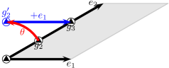
Figure 2: The second twisted sector in the $\text{G}_{2}$ two–torus has three fixed points (black dots) with corresponding constructing elements $g_{a}$, $a=1,2,3$. Under $\theta$ the fixed point of $g_{2}$ is mapped to $g_{2}^{\prime}$, which is equivalent to $g_{3}$ by a lattice translation $+e_{1}$. Hence, the constructing elements $g_{2}$ and $g_{3}$ belong to the same conjugacy class.

As explained above, the geometrical properties of the massless strings are encoded in $\Ket{g}$, where we identify the fixed point $f_{g}$ with the constructing element $g\in\mathbbm{S}$. While $g$ transforms, in general, non–trivially under the action of $h\in\mathbbm{S}$,

$$g~{}\xmapsto{h}~{}h\cdot g\cdot h^{-1}=g^{\prime}\;,$$ (15)

the conjugacy class

$$[g]~{}=~{}\{h\cdot g\cdot h^{-1}\;|\;h\in\mathbbm{S}\}$$ (16)

is by definition invariant under conjugation. We now construct the corresponding “geometrical eigenstate” $\Ket{[g]}$, which is, up to a phase, invariant under all space–group transformations such that the full physical state (5) is invariant under the action of every $h\in\mathbbm{S}$. This is achieved by building infinite linear combinations of orbifold–equivalent fixed points, or, equivalently, by summing over all elements of the conjugacy class,

$$\Ket{[g]}~{}=~{}\sum_{h}\mathrm{e}^{-2\pi\,\mathrm{i}\,\gamma(g,h)}\,\Ket{h\cdot g\cdot h^{-1}}\;.$$ (17)

Here the $\gamma(g,h)$ denote phases that are crucial for rendering $\Ket{[g]}$ an eigenstate w.r.t. all space–group transformations, $h\in\mathbbm{S}$ is chosen such that each term $\Ket{h\cdot g\cdot h^{-1}}$ appears once in the summation and we suppress the normalization. This is a natural extension of the usual linear combination of fixed points that are mapped to each other via the twist, e.g. in the second twisted sector of $\mathbbm{Z}_{6}$–II the $\text{G}_{2}$ torus contains three fixed points, two of them are identified on the orbifold (cf. the discussion in [2, 3, 11]), see figure 2. However, in contrast to the traditional linear combinations, the new geometrical eigenstates are eigenstates of the full space group as we will see in more detail later, i.e. for any $h\in\mathbbm{S}$ one obtains

$$\Ket{[g]}~{}\xmapsto{h}~{}\mathrm{e}^{2\pi\,\mathrm{i}\,\gamma(g,h)}\,\Ket{[g]}\;,$$ (18)

where $\gamma(g,h)\equiv 0$ if $g\cdot h=h\cdot g$. Here and in what follows “$\equiv$” means equal modulo 1. Note that (17) also implies a redefinition of the twist fields $\boldsymbol{\sigma}_{g}$, which can be expressed as an analogous sum. For fixed $g\in\mathbbm{S}$ the geometrical phase $\gamma(g,h)$ is a homomorphism from the space group $\mathbbm{S}$ to $\mathbbm{Z}_{6}$, i.e.  $\gamma(g,h_{1}\cdot h_{2})\equiv\gamma(g,h_{1})+\gamma(g,h_{2})$. Thus, for $h=(\theta^{\ell},m_{\alpha}\,e_{\alpha})$ one has

$$\gamma(g,h)~{}\equiv~{}\ell\,\gamma(g,\theta)+m_{\alpha}\,\gamma(g,e_{\alpha})\;,$$ (19)

where we define $\gamma(g,\theta):=\gamma\bigl{(}g,(\theta,0)\bigr{)}$ and $\gamma(g,e_{\alpha}):=\gamma\bigl{(}g,(\mathbbm{1},e_{\alpha})\bigr{)}$. We demand that the full physical state $\Ket{p_{\mathrm{sh}},q_{\mathrm{sh}},\widetilde{N},\widetilde{N}^{*},g}$ of equation (5) be invariant under a transformation with $h$. This translates to the condition

$$p_{\text{sh}}\cdot V_{h}-\left(q_{\text{sh}}+\Delta\widetilde{N}\right)\cdot v_{h}-\frac{1}{2}\left(V_{g}\cdot V_{h}-v_{g}\cdot v_{h}\right)+\gamma(g,h)~{}\stackrel{{\scriptstyle!}}{{\equiv}}~{}0\;,$$ (20)

allowing us to compute $\gamma(g,\theta)$ and $\gamma(g,e_{\alpha})$ by choosing appropriate $h$.

The crucial observation is now that the geometrical eigenstates $\Ket{[g]}$ are eigenstates with respect to a sublattice rotation $\theta^{(j)}$, which is not an element but an automorphism of $\mathbbm{S}$. Acting with $\theta^{(j)}$ on $\Ket{[g]}$ yields a phase,

$$\Ket{[g]}~{}\xmapsto{\theta^{(j)}}~{}\mathrm{e}^{2\pi\,\mathrm{i}\,\gamma(g,\theta^{(j)})}\,\Ket{[g]}\;.$$ (21)

This is because, as we will show explicitly below, in its action on $\Ket{[g]}$, $\theta^{(j)}$ is equivalent to an appropriate space–group transformation $h\in\mathbbm{S}$. In other words, $\theta^{(j)}$ is a conjugacy class preserving automorphism of $\mathbbm{S}$ (at least for $\mathbbm{Z}_{6}$–II). Therefore, the phase $\gamma\left(g,\theta^{(j)}\right)$ can be expressed in terms of $\gamma(g,\theta)$ and $\gamma(g,e_{\alpha})$.

As we have discussed above equation (12), sublattice rotations also imply a transformation of the shifted $\mathrm{SO}(8)$ momenta $q_{\mathrm{sh}}$ and the oscillator numbers $\Delta\widetilde{N}^{j}$. Taking into account all transformations under sublattice rotations and using that $(r_{j})^{j}=1/N^{j}$, the proper $R$ charges are thus defined as

$$R^{j}~{}=~{}q_{\text{sh}}^{j}+\Delta\widetilde{N}^{j}-N^{j}\,\gamma(g,\theta^{(j)})\;,$$ (22)

whose sum must equal $-1$ (modulo the order $N^{j}$ of the corresponding discrete sublattice rotation) in order for the correlator equation (7) to be invariant, i.e. $\sum_{a=1}^{L}R^{j}_{a}=-1\mod N^{j}$ for $j=1,2,3$. As in equation (13), these charges need to be multiplied by $(-6,-6,-2)$ in order to make the charges of all fields and of the superspace coordinate integer. This charge assignment is valid in the general case including non–trivial Wilson lines. In the simplified case without Wilson lines it differs by a sign from the previously derived expression in [5].

In what follows, we discuss this in detail starting with sublattice rotations first in the $\mathrm{SU}(3)$ and second in the $\mathrm{SU}(2)^{2}$ two–torus. In these cases, it is sufficient to construct the infinite linear combinations for the geometrical eigenstates for each two–torus separately. Finally, we perform the sublattice rotation in the $\mathrm{G}_{2}$ two–torus.

2.3.1 $\boldsymbol{\mathbbm{T}^{2}_{\mathrm{SU}(3)}/\mathbbm{Z}_{3}}$ sublattice rotation

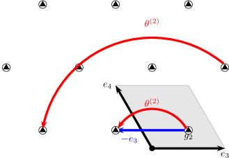
Figure 3: Visualization of the geometrical eigenstate $\Ket{[g_{2}]}$ of equation (23). One performs a sum over all equivalent fixed points in covering space weighted by appropriate $\gamma$ phase factors. The sublattice rotation $\theta^{(2)}$ is, for $g_{2}$, geometrically equivalent to a lattice translation by $-e_{3}$ up to three times a lattice translation.

Let us consider the second two–torus, where $\mathbbm{Z}_{6}$–II acts as $\mathbbm{Z}_{3}$. In the first ($k=1$) and fourth ($k=4$) twisted sectors there are three fixed points. Their constructing elements read $g_{a}=(\theta^{k},n_{3}\,e_{3}+n_{4}\,e_{4})$, where $k=1,4$ and $a=1,2,3$ for $(n_{3},n_{4})=(0,0),(1,0),(1,1)$, respectively, see figure 1(b). The associated geometrical eigenstates $\Ket{[g_{a}]}$ are obtained by taking infinite linear combinations, i.e.

$$\Ket{[g_{a}]}~{}=~{}\sum_{m_{3},m_{4}}\mathrm{e}^{-2\pi\,\mathrm{i}\,(m_{3}+m_{4})\,\gamma(g_{a},e_{3})}\,\Ket{\bigl{(}\theta^{k},(n_{3}+m_{3}+m_{4})\,e_{3}+(n_{4}+2m_{4}-m_{3})\,e_{4}\bigr{)}}\;,$$ (23)

with $\gamma(g,e_{3})\in\{0,\nicefrac{{1}}{{3}},\nicefrac{{2}}{{3}}\}$. Here we sum over all equivalent fixed points in the covering space, see figure 3. We can verify that these three states $\Ket{[g_{a}]}$ are eigenstates of the full space group by letting some arbitrary space group element $h$ act on $\Ket{[g_{a}]}$. Then each constructing element $g$ in the linear combination is mapped to $h\cdot g\cdot h^{-1}$ and, consequently, $\Ket{[g_{a}]}$ is mapped to itself times a phase. For example, under a general translation $h=(\mathbbm{1},s_{3}\,e_{3}+s_{4}\,e_{4})$ the geometrical eigenstate $\Ket{[g_{a}]}$ picks up a phase

$$\Ket{[g_{a}]}~{}\xmapsto{h=(\mathbbm{1},s_{3}\,e_{3}+s_{4}\,e_{4})}~{}\mathrm{e}^{2\pi\,\mathrm{i}\,(s_{3}+s_{4})\,\gamma(g_{a},e_{3})}\,\Ket{[g_{a}]}\;.$$ (24)

The crucial observation is now that, under a sublattice rotation $(\theta^{(2)},0)$, $\Ket{[g_{a}]}$ also gets mapped to itself up to a phase,

$$\Ket{[g_{a}]}~{}\xmapsto{(\theta^{(2)},0)}~{}\mathrm{e}^{-2\pi\,\mathrm{i}\,(n_{3}+n_{4})\,\gamma(g_{a},e_{3})}\,\Ket{[g_{a}]}\;.$$ (25)

For the case of $\Ket{[g_{2}]}$, this is illustrated in figure 3, where we see that any $g_{2}$–equivalent fixed point gets shifted by $-e_{3}$ up to three times a lattice translation. The shift by $-e_{3}$ induces, in the presence of a Wilson line, a non–trivial phase while, due to the Wilson line quantization and modular invariance conditions, three times a lattice translation does not lead to a phase. Thus, we find that $\gamma(g_{a},\theta^{(2)})=-(n_{3}+n_{4})\,\gamma(g_{a},e_{3})$ is the contribution to the $R$ charge under a rotation $r_{2}=(0,0,\frac{1}{3},0)$ for a state from the $k=1,4$ sectors. For a state from the $k=2,5$ sector we get $\gamma(g_{a},\theta^{(2)})=(n_{3}+n_{4})\,\gamma(g_{a},e_{3})$. Finally, for $k=0,3$ we have $\gamma(g_{a},\theta^{(2)})=0$. Combining these results we obtain

$$\gamma(g_{a},\theta^{(2)})~{}\equiv~{}-k\,(n_{3}+n_{4})\,\gamma(g_{a},e_{3})$$ (26)

for a state with constructing element $g_{a}=(\theta^{k},n_{3}\,e_{3}+n_{4}\,e_{4})$.

Altogether we have seen that the sublattice rotation $\theta^{(2)}$, whose gauge embedding is not defined (because $\theta^{(2)}\not\in\mathbbm{S}$), can be traded against a translation, for which we know the gauge embedding. From this we can infer the transformation properties of the full state $\Ket{p_{\mathrm{sh}},q_{\mathrm{sh}},\widetilde{N},\widetilde{N}^{*},g}$ (see equation (5)). Demanding that $\Ket{p_{\mathrm{sh}},q_{\mathrm{sh}},\widetilde{N},\widetilde{N}^{*},g}$ be invariant under all space group transformations allowed us then to compute via equation (20) the $\gamma$ phases, which enter the $R$ charges (22).

2.3.2 $\boldsymbol{\mathbbm{T}^{2}_{\mathrm{SU}(2)\times\mathrm{SU}(2)}/\mathbbm{Z}_{2}}$ sublattice rotation

Next, consider the two–torus $\mathbbm{T}^{2}_{\mathrm{SU}(2)\times\mathrm{SU}(2)}$, where $\theta$ acts as $\mathbbm{Z}_{2}$. The analysis is analogous to the one above. In this torus there are four fixed points (if $k$ is odd) with constructing elements

$$g_{a}~{}=~{}(\theta^{k},n_{5}\,e_{5}+n_{6}\,e_{6})\;,$$ (27)

where $(n_{5},n_{6})=(0,0),(0,1),(1,0)$ or $(1,1)$ for $a=1,2,3,4$, respectively, see figure 1(c). Again, the associated geometrical eigenstates $\Ket{[g_{a}]}$ are obtained by taking infinite linear combinations, i.e.

$$\Ket{[g_{a}]}~{}=~{}\sum_{m_{5},m_{6}}\mathrm{e}^{-2\pi\,\mathrm{i}\,\bigl{(}m_{5}\,\gamma(g_{a},e_{5})+m_{6}\,\gamma(g_{a},e_{6})\bigr{)}}\,\Ket{\bigl{(}\theta^{k},(n_{5}+2m_{5})\,e_{5}+(n_{6}+2m_{6})\,e_{6}\bigr{)}}\;,$$ (28)

with $\gamma(g_{a},e_{5})\in\{0,\nicefrac{{1}}{{2}}\}$ and $\gamma(g_{a},e_{6})\in\{0,\nicefrac{{1}}{{2}}\}$. As before, under a general translation $h=(\mathbbm{1},s_{5}e_{5}+s_{6}e_{6})$ the geometrical eigenstate $\Ket{[g_{a}]}$ picks up a phase

$$\Ket{[g_{a}]}~{}\mapsto~{}\mathrm{e}^{2\pi\,\mathrm{i}\,\bigl{(}s_{5}\,\gamma(g_{a},e_{5})+s_{6}\,\gamma(g_{a},e_{6})\bigr{)}}\,\Ket{[g_{a}]}\;.$$ (29)

Furthermore, under a sublattice rotation $(\theta^{(3)},0)$, $\Ket{[g_{a}]}$ transforms with a phase,

$$\Ket{[g_{a}]}~{}\mapsto~{}\mathrm{e}^{2\pi\,\mathrm{i}\,\bigl{(}n_{5}\gamma(g_{a},e_{5})+n_{6}\gamma(g_{a},e_{6})\bigr{)}}\,\Ket{[g_{a}]}\;.$$ (30)

If $k$ is even, the sublattice rotation $\theta^{(3)}$ acts on a fixed torus (with $n_{5}=n_{6}=0$) and hence $\gamma(g_{a},\theta^{(3)})=0$. Combining these results we obtain

$$\gamma(g_{a},\theta^{(3)})~{}\equiv~{}n_{5}\,\gamma(g_{a},e_{5})+n_{6}\,\gamma(g_{a},e_{6})\;,$$ (31)

for a state with constructing element $g_{a}=(\theta^{k},n_{5}\,e_{5}+n_{6}\,e_{6})$.

Let us stress that our analysis in 2.3.1 and 2.3.2 can be applied to any orbifold with a $\mathbbm{Z}_{3}$ sublattice rotation in an $\mathrm{SU}(3)$ plane and/or $\mathbbm{Z}_{2}$ sublattice rotation in an $\mathrm{SU}(2)\times\mathrm{SU}(2)$ plane, thus allowing us to compute the proper $R$ charges for many other orbifold geometries.

2.3.3 $\boldsymbol{\mathbbm{T}^{2}_{\mathrm{G}_{2}}/\mathbbm{Z}_{6}}$ sublattice rotation

Last, we consider the first complex plane, where $\mathbbm{Z}_{6}$–II acts as $\mathbbm{Z}_{6}$. There are two ways to derive $\gamma(g,\theta^{(1)})$ in this case. First, we know that

$$\theta^{(1)}~{}=~{}\theta\cdot\left(\theta^{(2)}\right)^{-1}\cdot\left(\theta^{(3)}\right)^{-1}\;.$$ (32)

Hence, the phase of the geometrical eigenstate with constructing element $g=(\theta^{k},n_{\alpha}e_{\alpha})$ under a $\theta^{(1)}$ sublattice rotation is given by

$$\gamma(g,\theta^{(1)}) \equiv \gamma(g,\theta)-\gamma(g,\theta^{(2)})-\gamma(g,\theta^{(3)})$$ (33)

$$\equiv \gamma(g,\theta)+k\,(n_{3}+n_{4})\,\gamma(g,e_{3})-\bigl{(}n_{5}\,\gamma(g,e_{5})+n_{6}\,\gamma(g,e_{6})\bigr{)}\;.$$ (34)

The second possibility is the explicit construction of the full geometrical eigenstate, which yields the same result for $\gamma(g,\theta^{(1)})$, as expected.

2.3.4 Summary of $\boldsymbol{R}$ charges

In summary, the three $R$ charges of the $\mathbbm{Z}_{36}^{R}\times\mathbbm{Z}_{18}^{R}\times\mathbbm{Z}_{4}^{R}$ symmetry for a (twisted) state of the $\mathbbm{Z}_{6}$–II orbifold with constructing element $g=\left(\theta^{k},n_{\alpha}\,e_{\alpha}\right)$ read

$$R^{1} = -6\,\Bigl{[}q_{\text{sh}}^{1}+\Delta\widetilde{N}^{1}-6\,\gamma(g,\theta)$$ (35a)

$${}\hphantom{-6\,\Bigl{[}}{}-6\,k\,(n_{3}+n_{4})\,\gamma(g,e_{3})+6\,\bigl{(}n_{5}\,\gamma(g,e_{5})+n_{6}\,\gamma(g,e_{6})\bigr{)}\Bigr{]}\;,$$

$$R^{2} = -6\,\Bigl{[}q_{\text{sh}}^{2}+\Delta\widetilde{N}^{2}+3\,k\,(n_{3}+n_{4})\,\gamma(g,e_{3})\Bigr{]}\;,$$ (35b)

$$R^{3} = -2\,\Bigl{[}q_{\text{sh}}^{3}+\Delta\widetilde{N}^{3}-2\,\bigl{(}n_{5}\,\gamma(g,e_{5})+n_{6}\,\gamma(g,e_{6})\bigr{)}\Bigr{]}\;,$$ (35c)

where the superspace coordinate has $R$ charges $(3,3,1)$ and all $R$ charges are normalized to be integer. Note that the $\gamma$ charges vanish for untwisted fields. We have “tested” these $R$ charges for a huge set of randomly generated $\mathbbm{Z}_{6}$–II orbifold models with non–trivial Wilson lines [12] and found that the anomalies are always universal, i.e. can be cancelled by the dilaton. On the other hand, restricting to $W_{\alpha}=0$ and using the $R$ charges from [5], where the $N^{j}\,\gamma(g,\theta^{(j)})$ term appears with the opposite sign, leads to non–universal $R^{1}$ anomalies.

It is instructive to apply the three discrete $R$ transformations consecutively to some field $\Psi_{g}$. This results in a $\mathbbm{Z}_{36}$ phase $R_{g}$ given by

$$\frac{1}{36}R_{g}~{}=~{}-\frac{1}{36}\left(R^{1}+2R^{2}-9R^{3}\right)~{}\equiv~{}p_{\text{sh}}\cdot V-\frac{1}{2}\left(V_{g}\cdot V-v_{g}\cdot v\right)\;,$$ (36)

where we used the invariance condition equation (20). Now consider a coupling between states with constructing elements $g_{1}\ldots g_{L}$. One can see that the total $R$ transformation is trivial, i.e. $\frac{1}{36}\sum_{g}R_{g}\equiv 0$ by using gauge invariance, the point group selection rule, the space group selection rule in the second and third two–torus and finally modular invariance. Hence, the string selection rules are not independent and one could trade off, for example, one of the $R$ symmetries. That is, as also observed in [13], some of the symmetries are redundant; these redundancies can be eliminated with the methods discussed in [14].

One may also wonder if one could separate off the $\gamma$ contributions from the $R$ charges. At first glance, one may think the space–group selection rule implies that the $\gamma$–phases sum up to $0\mod 1$ since the product of the respective constructing elements has to yield the identity $(\mathbbm{1},0)$, and $\gamma\bigl{(}(\mathbbm{1},0),h\bigr{)}\equiv 0$ for all $h\in\mathbbm{S}$. However, for each constructing element $g\in\mathbbm{S}$ the sublattice rotations $\theta^{(i)}$ are, in general, equivalent to different space–group operations such that it is not generally possible to separate the $\gamma$ contributions.

3 Summary

We have re–derived the $R$ symmetries and charges for the $\mathbbm{Z}_{6}$–II orbifold with Wilson lines. As we have seen, the discrete $R$ symmetries originate from sublattice rotations of the orbifold accompanied by an analogous action on the right–mover. This yields the well–known contributions to the $R$ charges. By constructing states that are invariant under the full space group $\mathbbm{S}$ we were able to determine the transformation behavior of the twist fields under sublattice rotations, which are automorphisms but not elements of $\mathbbm{S}$. Separating the correlator of the vertex operators into a gauge part and a rest allowed us to determine necessary conditions for the correlators to be non–trivial, which can be rewritten as discrete $R$ symmetries. With our derivation, we confirm the statement of [5] that the $R$ charges have to be amended by appropriate $\gamma$ phases, disagree, however, in a sign. Further, our derivation allowed us to treat also the case of non–vanishing Wilson lines.

Using the correct definition of $R$ charges, equation (22), has important consequences for orbifold model building. First, $\mathbbm{Z}_{M}^{R}$ anomalies are now universal, as we have explicitly verified in thousands of $\mathbbm{Z}_{6}$–II orbifold models (including up to three non–trivial Wilson lines). In particular, the non–universal anomalies found in [4] are a consequence of the incorrect $R$ charges used in the analysis. Repeating the analysis with proper $R$ charges leads to universal anomalies, which can be cancelled by the dilaton. Further, the fact that [15] did find universal anomalies ignoring the $\gamma$ phases is, in particular, related to the simplicity of their models which is characterized by the absence of Wilson lines, such that the massless twisted states appear with degeneracy factors, thus rendering the anomaly coefficients universal “by accident”. Using proper $R$ charges has also important implications for heterotic orbifold phenomenology. In particular, if one compares couplings that are allowed by the incorrect vs. correct $R$ charges, one finds that many more couplings are allowed if one imposes the proper $R$ symmetries. As a consequence, vector–like exotics of MSSM–like constructions, such as those of [16, 17, 18], decouple at low orders and Yukawa textures are changed. At the same time, discrete $R$ symmetries (such as the $\mathbbm{Z}_{4}^{R}$ symmetry [19]) remain instrumental for suppressing the $\mu$ term and dangerous proton decay operators. Yet, clearly, the construction of vacua with residual discrete and/or approximate $R$ symmetries has to be revisited. This will be done elsewhere.

Although our presentation was focused on the $\mathbbm{Z}_{6}$–II orbifold based on factorizable tori, our derivation is general and can be extended to all symmetric (or geometric) orbifolds [20]. In particular, our analysis in sections 2.3.1 and 2.3.2 can be applied to any orbifold with a $\mathbbm{Z}_{3}$ sublattice rotation in an $\mathrm{SU}(3)$ plane and/or $\mathbbm{Z}_{2}$ sublattice rotation in an $\mathrm{SU}(2)\times\mathrm{SU}(2)$ plane, thus allowing us to compute the proper $R$ charges for many other orbifold geometries. This analysis will be carried out elsewhere.

Acknowledgements.

We would like to thank Robert Richter for important discussions. S.R–S. thanks the ICTP for hospitality and the support received through the ICTP Junior Associateship Scheme. M.R. would like to thank the UC Irvine, where part of this work was done, for hospitality. The work of H.P.N. was supported by SFB-Transregio TR33 “The Dark Universe” (Deutsche Forschungsgemeinschaft) and the European Union 7th network program “Unification in the LHC era” (PITN-GA-2009-237920). This work was partially supported by the DFG cluster of excellence “Origin and Structure of the Universe”. P.V. is supported by SFB grant 676. This research was done in the context of the ERC Advanced Grant project “FLAVOUR” (267104). S.R–S. is partially supported by CONACyT grant 151234 and DGAPA-PAPIIT grant IB101012-RR181012.

References

- [1] L. J. Dixon, J. A. Harvey, C. Vafa, and E. Witten, Nucl. Phys. B261 (1985), 678.
- [2] L. J. Dixon, J. A. Harvey, C. Vafa, and E. Witten, Nucl. Phys. B274 (1986), 285.
- [3] T. Kobayashi, S. Raby, and R.-J. Zhang, Nucl.Phys. B704 (2005), 3, arXiv:hep-ph/0409098 [hep-ph].
- [4] T. Araki et al., Nucl. Phys. B805 (2008), 124, arXiv:0805.0207 [hep-th].
- [5] N. G. Cabo Bizet, T. Kobayashi, D. K. Mayorga Peña, S. L. Parameswaran, M. Schmitz, et al., JHEP 1305 (2013), 076, arXiv:1301.2322 [hep-th].
- [6] S. Hamidi and C. Vafa, Nucl. Phys. B279 (1987), 465.
- [7] L. J. Dixon, D. Friedan, E. J. Martinec, and S. H. Shenker, Nucl. Phys. B282 (1987), 13.
- [8] A. Font, L. E. Ibáñez, H. P. Nilles, and F. Quevedo, Nucl. Phys. B307 (1988), 109, Erratum ibid. B310.
- [9] A. Font, L. E. Ibáñez, H. P. Nilles, and F. Quevedo, Phys. Lett. B210 (1988), 101, Erratum ibid. B213.
- [10] A. Font, L. E. Ibáñez, F. Quevedo, and A. Sierra, Nucl. Phys. B331 (1990), 421.
- [11] W. Buchmüller, K. Hamaguchi, O. Lebedev, and M. Ratz, Nucl. Phys. B785 (2007), 149, hep-th/0606187.
- [12] H. P. Nilles, S. Ramos-Sánchez, P. K. Vaudrevange, and A. Wingerter, Comput.Phys.Commun. 183 (2012), 1363, arXiv:1110.5229 [hep-th], web page http://projects.hepforge.org/orbifolder/.
- [13] W. Buchmüller and J. Schmidt, Nucl. Phys. B807 (2009), 265, arXiv:0807.1046 [hep-th].
- [14] B. Petersen, M. Ratz, and R. Schieren, JHEP 08 (2009), 111, arXiv:0907.4049 [hep-ph].
- [15] T. Araki, K.-S. Choi, T. Kobayashi, J. Kubo, and H. Ohki, Phys.Rev. D76 (2007), 066006, arXiv:0705.3075 [hep-ph].
- [16] O. Lebedev, H. P. Nilles, S. Raby, S. Ramos-Sánchez, M. Ratz, P. K. S. Vaudrevange, and A. Wingerter, Phys. Lett. B645 (2007), 88, hep-th/0611095.
- [17] O. Lebedev, H. P. Nilles, S. Raby, S. Ramos-Sánchez, M. Ratz, P. K. S. Vaudrevange, and A. Wingerter, Phys. Rev. D77 (2007), 046013, arXiv:0708.2691 [hep-th].
- [18] R. Kappl, H. P. Nilles, S. Ramos-Sánchez, M. Ratz, K. Schmidt-Hoberg, and P. K. Vaudrevange, Phys. Rev. Lett. 102 (2009), 121602, arXiv:0812.2120 [hep-th].
- [19] H. M. Lee, S. Raby, M. Ratz, G. G. Ross, R. Schieren, K. Schmidt-Hoberg, and P. K. Vaudrevange, Phys.Lett. B694 (2011), 491, arXiv:1009.0905 [hep-ph].
- [20] M. Fischer, M. Ratz, J. Torrado, and P. K. Vaudrevange, JHEP 1301 (2013), 084, arXiv:1209.3906 [hep-th].